Zeina Baalbaki A thesis submitted to McGill University in partial fulfillment of the requirements of the

degree of Doctor of Philosophy

Department of Chemical Engineering McGill University Montreal, Canada

August 2016

©Copyright Zeina Baalbaki 2016

ABSTRACT

The presence of contaminants of emerging concern (CECs) in the aquatic environment and the associated proven toxic impacts have increasingly alarmed researchers. The discharge of wastewater into surface water was identified as the major source for the release of CECs into the environment. Despite the available data on the removal of CECs in wastewater treatment plants (WWTPs) in the literature, previous studies had several shortcomings, resulting in an inaccurate prediction of the CEC fate. This PhD project aimed at monitoring the fate of CECs in different treatment steps with special consideration to the hydrodynamics of the treatment units and adsorption to sludge. The project also aimed at developing and calibrating a model to predict the fate of target CECs in the most widespread secondary treatment technology: the activated sludge process. Among the various classes of CECs, this thesis focused on the widely consumed pharmaceuticals, personal care products, drugs of abuse, hormones, stimulants and artificial sweeteners based on evidences of their presence in treated wastewater implying their inefficient removal during treatment. Recently, the hydraulic characteristics of WWTPs were demonstrated to bias the calculations of CEC removal if not accounted for. To address this issue, the fractionated approach that integrates hydraulic modelling and improved sampling strategies was recently proposed. In order to verify the capability of the fractionated approach at capturing the hydraulic differences, the temperature and electric conductivity of wastewater were used as tracers to model the hydraulics of two full-scale WWTPs. Results demonstrated that a distinctive model was necessary to describe the hydraulics in each WWTP, requiring different number of days for sampling, as well as different CEC removal calculations. In order to explore the contribution of the different fate pathways to the removal of CEC during wastewater treatment, a sampling campaign was performed in a WWTP using an optimized sampling strategy based on the fractionated approach to collect and chemically analyze both wastewater and sludge samples. This allowed performing a mass balance on the incoming load of CECs, which was carried out for the first time with consideration to the hydraulic characteristics. Results indicated that for 21 out of 24 investigated CECs, degradation was the major removal process, with sorption accounting for <10% of the input CEC load fate in the

primary clarifier and <5% in the activated sludge process. Most target CECs (22 out of 25) were relatively persistent in rotating biological contactors and sand filtration compared to activated sludge treatment. In order to predict the fate of CECs, a fate model based on the widespread Activated Sludge Model No. 2d (ASM2d) was further modified to better describe the CEC fate processes in aeration tanks. The state-of-the-art Bürger-Diehl secondary clarifier model was extended to include the CEC fate processes for the first time. The resulting secondary treatment model was calibrated to predict the fate of four target CECs that belong to different classes and undergo different fate processes. Results from global sensitivity analysis indicated that depending on the contaminant’s properties, a different set of parameters deserved more attention. Further, dynamic sensitivity analysis should be taken into consideration in future sampling campaigns for model calibration.

RÉSUMÉ

La présence de contaminants d’intérêt émergent (CIE) dans l’environnement aquatique et les impacts toxiques associés à leur présence alarment de plus en plus les chercheurs. Le rejet d’eaux usées dans les eaux de surface a été identifié comme la source principale du relâchement de ces CIE dans l'environnement. Malgré les données disponibles dans la littérature relativement à l’enlèvement des CIE dans les stations d’épuration des eaux usées (STEP), plusieurs lacunes de ces études doivent être résolues. Ce projet de doctorat visait à évaluer le devenir des CIE dans les différentes étapes de traitement, en portant une attention particulière à l’hydrodynamique des unités de traitement. Le projet visait également à développer et calibrer un modèle de prédiction du devenir des CIE cibles en cours de traitement par boues activées, la technologie de traitement secondaire la plus répandue. Parmi les différentes classes de CIE, cette thèse se concentre sur les produits pharmaceutiques de grande consommation, les produits de soins personnels, les drogues, les hormones, les stimulants et les édulcorants artificiels. La sélection des CIE cibles s’est basée sur leur présence démontrée dans les eaux usées traitées impliquant leur élimination inefficace pendant le traitement. Récemment, il a été démontré que les caractéristiques hydrauliques des STEP influencent les calculs d'enlèvement des CIE s’ils ne sont pas prises en compte. Pour résoudre ce problème, l'approche fractionnée qui intègre une modélisation hydraulique et des stratégies d'échantillonnage améliorées a été récemment proposée. La conductivité électrique et la température ont été utilisées comme traceurs pour modéliser le comportement hydraulique de deux stations d'épuration, permettant ainsi de vérifier l’efficacité de l'approche fractionnée à capter les différences hydrauliques. Les résultats ont démontré qu’un modèle distinct est nécessaire pour décrire l'hydraulique dans chaque station d'épuration, imposant donc un nombre de jours différent pour l’échantillonnage ainsi que des calculs différents d'élimination des CIE. Afin d'explorer la contribution des différentes voies d’élimination des CIE au cours du traitement des eaux usées, une campagne d'échantillonnage a été effectuée dans une station d'épuration en utilisant une stratégie d'échantillonnage optimisée basée sur l'approche fractionnée. Les échantillons d’eau et de boue recueillis et analysés au cours de cette campagne ont permis d'effectuer un bilan de matière sur la charge entrante de CIE, ceci étant réalisé pour la première

fois en tenant compte des caractéristiques hydrauliques. Les résultats indiquent que pour 21 des 24 CIE, la dégradation a été le processus principal d'élimination, avec une sorption représentant <10% de l’élimination des charges entrantes de CIE au clarificateur primaire et <5% au procédé de boues activées. La plupart des CIE cibles (22 sur 25) étaient relativement persistants dans les contacteurs biologiques rotatifs et la filtration sur sable par rapport au traitement par boues activées. Afin de prédire le devenir de CIE au cours du traitement des eaux usées, un modèle basé sur le modèle connu de boues activées No.2d (ASM2d) a été développé afin de mieux décrire les processus qui affectent les CIE dans les bassins d'aération. Les processus d’élimination des CIE ont été ajoutés au modèle Bürger-Diehl de décantation pour la première fois. Les mesures de concentration des CIE ont été utilisées pour calibrer le modèle de traitement secondaire afin de prédire le devenir de quatre CIE cibles qui appartiennent à des classes différentes de CIE et subissent différents processus d’élimination. Les résultats de l'analyse globale de sensibilité ont indiqué qu'un ensemble de paramètres différents méritent une attention particulière selon les propriétés des CIE. L’analyse de sensibilité dynamique pourrait être mis à profit dans des campagnes futures de mesure visant la calibration de modèles.

ACKNOWLEDGEMENTS

I would like to express my gratitude to my supervisors: Prof. Viviane Yargeau and Prof. Peter Vanrolleghem. Thanks to Prof. Viviane Yargeau for accepting me for a direct entry to the PhD and providing me with the tools to grow as a researcher. Her knowledge, encouragement and inspirational attitude were essential for the completion of my PhD. Also, I would like to express my gratitude to Prof. Peter Vanrolleghem who with his wide knowledge, provided valuable contribution to the modelling component of my project and with his thorough reviews, was determined that the papers get finalized in best form. I am truly honored to be mentored by both of my supervisors and enriched by their useful insights and feedbacks. I wish to thank my co-authors: Prof. Chris Metcalfe and Tamanna Sultana for providing valuable insights on the papers. Also thanks to Thomas Maere and Elena Torfs for their vital help on the modelling aspect of the project. I am grateful to Mr. Marco Pineda for his help with the chemical analysis of Guelph samples and for his dedication to provide me with valuable deep understanding of the instrument and the methods. I would also wish to acknowledge the support received from the staff at the WWTPs. In particular, the help received from Mr. Gerald Atkinson and Mr. Greg Jorden at the Guelph WWTP in answering my numerous questions was crucial for the accomplishment of the modelling work of this project. I am also grateful to all the past and current 3Cs group members who helped during the demanding sampling campaigns: Angela, Jonathan, Shadi, Melissa, Michael, Meghan, Paul, Liam and Sarah. Also, thanks to Francois for kindly correcting the French version of the abstract. Despite the incredibly long working hours, my three years at McGill were made enjoyable by the different people who have made this experience worth it. First, special thanks to Zeina Jendi, who was the only person I had known in Canada when I first arrived three years ago, as she helped me immensely and introduced me to the adventure ahead. Thanks to Meghan for sharing with me the most pleasant and most stressful moments of this PhD experience, both of which were filled with relieving humour. Thanks to Shaqa, Evelyne and Serene whose support, encouragement and calming words made the seemingly unending PhD possible. Last but not least, thanks to my parents who have always believed in me and have skilfully engraved in my mind that with dedication, any situation could be turned into one’s best advantage.

Funding: Funding to this PhD project was available from the Natural Sciences and Engineering Research Council of Canada (NSERC) through the Strategic Grants Program. I also wish thank the McGill Engineering Doctoral Award, the Graduate Excellence Fellowship and the Chair’s Discretionary Award for providing me with scholarships.

TABLE OF CONTENTS

ABSTRACT

RÉSUMÉ

ACKNOWLEDGEMENTS

TABLE OF CONTENTS

LIST OF FIGURES

LIST OF TABLES

ABBREVIATIONS AND UNITS

CONTRIBUTION OF AUTHORS

1. INTRODUCTION

2. LITERATURE REVIEW

2.3.3.1. Primary settling and activated sludge

3. OBJECTIVES

4. ESTIMATING REMOVAL OF CONTAMINANTS OF EMERGING CONCERN

FROM WASTEWATER TREATMENT PLANTS: THE CRITICAL ROLE OF

WASTEWATER HYDRODYNAMICS

5. FATE AND MASS BALANCE OF CONTAMINANTS OF EMERGING CONCERN

DURING WASTEWATER TREATMENT DETERMINED USING THE

FRACTIONATED APPROACH

6. DYNAMIC MODELLING OF SOLIDS IN FULL-SCALE ACTIVATED SLUDGE

PLANT PRECEDED BY CEPT AS A BASIC STEP FOR MICROPOLLUTANT

REMOVAL MODELLING

7. PREDICTING THE FATE OF MICROPOLLUTANTS DURING WASTEWATER

TREATMENT: CALIBRATION AND SENSITIVITY ANALYSIS

8. ORIGINAL COUNTRIBUTIONS

9. CONCLUSIONS

10. RECOMMENDATIONS

11. REFERENCES

APPENDIX I: SETTLER MODELS

LIST OF FIGURES

Figure 2.1 Chemical structures of the studied pharmaceuticals, their molecular weight (MW, g/mol), pKa, log Kow and their common trade names. pKa and Log Kow values were obtained from the National Center for Biotechnology Information (2004).

Figure 2.2 Chemical structure and molecular weight (MW, g/mol) of the two major metabolites of carbamazepine studied. Log Kow values obtained from National Center for Biotechnology Information (2004) N.A.:unavailable data.

Figure 2.3 Chemical structure, molecular weight (MW, g/mol) and properties of the studied drugs of abuse. pKa and Log Kow values obtained from National Center for Biotechnology Information (2004) N.A.:unavailable data.

Figure 2.4 Chemical structure, molecular weight (MW, g/mol) and properties of the studied metabolite of cocaine (benzoylecgonine) and methadone (EDDP). pKa and Log Kow values obtained from National Center for Biotechnology Information (2004). N.A.:unavailable data.

Figure 2.5 Chemical structure, molecular weight (MW, g/mol) and chemical properties of estrone and androstenedione. pKa and Log Kow values obtained from National Center for Biotechnology Information (2004). N.A.:unavailable data.

Figure 2.6 Chemical structure, molecular weight (MW, g/mol) and chemical properties of sucralose, caffeine and triclosan. pKa and Log Kow values obtained from National Center for Biotechnology Information (2004), except for sucralose (Busetti et al., 2015; Subedi & Kannan, 2014a). N.A.:unavailable data.

Figure 2.7 Illustration of the concept of the residence time distribution and its impact on sampling strategies.

Figure 4.1 Observed (recorded) and predicted (simulated) conductivity trends in (a) WWTP A and (b) WWTP B at different locations (PI: influent to primary clarification, PE: effluent of primary clarification, AE: effluent of aeration, SE: effluent of secondary clarification).

Figure 4.2 Simulated response to a hypothetical CEC 24-h step input (a) Input applied on first, second and third days of sampling separately to the best-fit hydraulic model of the activated sludge unit in WWTP A; (b) Input applied on first, second, third and fourth sampling days separately to the best-fit hydraulic model of the activated sludge unit in WWTP B.

Figure 4.3 Mass loads of target CECs in influent (based on load fractions of two days) and effluent (load on the last day) of the primary clarifier of the WWTP A. Day 1,2,3 represent first, second and third sampling day, respectively. Error bars = one standard deviation of 3 replicates. Sucralose is not shown in this graph, as it has a significantly higher range of mass loads values.

Figure 4.4 Mass loads of target CECs in influent (based on load fractions of two days) and effluent (load on last day) of the activated sludge unit at the WWTP A. Day 1,2,3 represent first, second and third sampling days, respectively. Error bars = one standard deviation of 3 replicates. * denotes compounds with effluent concentration < LOD or LOQ, where mass loads were considered 0 in this graph. Sucralose is not shown in this graph, as it has a significantly higher range of mass loads values.

Figure 4.5 Mass loads of target CECs in influent (based on load fractions of 3 days) and effluent (load on last day) of the activated sludge unit at the WWTP B. Day 1,2,3,4 represent first, second, third and fourth sampling days, respectively. Error bars = one standard deviation of 3 replicates. * denotes compounds with effluent concentration < LOD or LOQ, where mass loads were considered 0 in this graph. Caffeine, sucralose and acetaminophen are not shown in this graph, as they have a significantly higher range of mass loads values.

Figure 5.1 Schematic of the WWTP. Lines 1-4 correspond to the four lines of primary and secondary treatment. Red marks represent locations where conductivity probes were deployed and aqueous samples were collected. Green marks represent locations where sludge samples were collected.

Figure 5.2 Estimated removal efficiencies (%) of target CECs. The removal efficiency was based on the incoming load to each treatment unit. ***, **, * denote compounds that were <LOD or <LOQ in the effluent of the activated sludge, RBC and sand filter, respectively, so removal was based on LOD (for <LOD) or LOQ (for <LOQ) and may be higher than reported here. Absence of a column indicates that either the removal was negative or the compound was <LOD or <LOQ in the influent to the treatment unit.

Figure 5.3 Input reference mass loads (g/d) of target CECs into the primary clarifier assigned into three main fate pathways: (bio)degraded, discharged with primary sludge and discharged with the primary effluent with the % contribution of each pathway indicated in the corresponding column (COC: cocaine, BG: benzoylecgonine, MTD: methadone). For

caffeine (not shown due to the high mass loads): 14% biodegraded, 2% sorbed to primary sludge and 84% in the effluent.

Figure 5.4 Input reference mass loads of target CECs into activated sludge assigned into three main fate pathways: (bio)degraded, discharged with waste activated sludge and discharged with the secondary effluent with % of each pathway in columns (COC: cocaine, BG: benzoylecgonine, MTD: methadone). For ibuprofen and amphetamine, the concentration in the effluent was <LOQ, so the LOQ was used for calculations. For caffeine (not shown due to the high mass loads): 92% biodegraded and 8% in the effluent.

Figure 5.5 Mass loads of carbamazepine and its two investigated metabolites (CMZ-DiOH & CMZ-EP) in both the input (reference load) and the output of the primary clarifier, secondary treatment, RBCs and sand filter. The numeric values of the load are presented in the columns.

Figure 5.6 Schematic illustrating the information (measurements) of streams used for mass balance calculations.

Figure 5.7 Effluent tracer (electrical conductivity (μS/cm)) trends measured (blue) and predicted by the best-fitting hydraulic model (dashed red) throughout four consecutive days for: a) primary clarifier, b) aeration tanks, c) RBCs and d) sand filter.

Figure 6.1 Schematic of the Guelph WWTP. Wastewater streams are represented by continuous

lines and sludge streams by dashed lines.

Figure 6.2 Measured and predicted MLSS concentrations. The latter was obtained using the

Takács model and standard settling parameters: Case A: COD-based TSS in the influent,

Case B: Measured TSS in influent, Case C: 1.35 x measured TSS in the influent. The time

axis is from July 2013 to June 2014.

Figure 6.3 Measured and predicted TSS concentrations in waste sludge (WAS TSS) after input

solids characterization. The time axis is from July 2013 to June 2014.

Figure 6.4 Comparison of predicted effluent TSS concentrations obtained using the Takács and

Bürger-Diehl settler models with different parameters (Table 6.5). The time axis is from

July 2013 to June.

Figure 6.5 Measured and predicted conventional pollutant concentrations: a) nitrate, b) ammonia

and c) COD in the secondary effluent using the best-fit model. The time axis is from July

2013 to June.

Figure 6.6 Polynomial fit of measured COD (upper) and TKN (lower) in the primary effluent. Time axis is from July 2013 to June 2014.

Figure 7.1 Schematic of the investigated full-scale activated sludge unit. Sampling locations are indicated with a cross sign (PE: primary effluent, AE: aeration effluent, SE: secondary effluent, WAS: waste activated sludge) and the corresponding measurements taken (SMP and XMP indicate measurement of the micropollutant concentration in aqueous and particulate phases, respectively).

Figure 7.2 Predicted soluble caffeine concentration in the two secondary clarifier outputs: a) secondary waste sludge and b) secondary effluent, accounting for both sorption and biodegradation (Ads+ bio), only sorption (Ads) or none of the fate processes (None).

Figure 7.3 Impact of changing on the concentration of caffeine in a) secondary effluent (soluble) and b) WAS (particulate) at different kbio values (L/(gSS.day)) and at fixed ksor=5 L/(gSS.day). XMP-WAS was plotted on a logarithmic axis due to the sharp variations induced by changing kbio and .

Figure 7.4 Normalized represented as ratio of the minimum for a) caffeine, b) ibuprofen, c) androstenedione, d) triclosan as a result of varying each model parameter: (first row), (second row) and (third row).

Figure 7.5 Measured (meas.) influent concentrations as well as measured and simulated (sim.) soluble secondary effluent concentrations for a) caffeine, b) ibuprofen, c) triclosan, d) androstenedione. The flow-average of simulated values are shown as (avg sim.). For ibuprofen only, the soluble effluent concentrations are displayed on a separate secondary axis since values are much lower than in the input.

Figure 7.6 Measured and simulated concentrations of each micropollutant in secondary waste sludge (ng/g). The error bars represent the standard deviations obtained from measurements on the four days of sampling for both simulations and measurements. P-values from the two-sample t-test represent the match between the measured and simulated concentration of the micropollutant.

Figure 7.7 Dynamic local sensitivity of the MP soluble concentrations (upper graphs) and particulate concentrations (lower graphs) in different locations: AE, SE and WAS to small perturbations in the three parameters for caffeine (a & b) and triclosan (c & d).

LIST OF TABLES Table 2.1 Selected pharmaceuticals and their human excretion percentage, their detection ratio

(DR) and detection frequency (DF) in effluent wastewater, as well as their mean concentration in surface water

Table 2.2 Selected drugs of abuse and their human excretion percentage, concentrations in effluent wastewater and in surface water.

Table 2.3 Concentrations of the target CECs in influent wastewater to WWTPs and the range of their overall removal efficiencies in WWTPs as reported by several past studies carried out in different countries.

Table 2.4 Removal of CECs obtained in different activated sludge units and primary clarifiers, evaluated separately.

Table 2.5 Sampling techniques used for the studies shown in Table 2.4, including the type of sample (grab or 24-h composite, flow-proportional or time-proportional), the consideration of residence time distribution (RTD) or hydraulic residence time (HRT) and the inclusion of sludge samples in the analysis.

Table 2.6 values reported in the literature for the target CECs for primary and waste secondary sludge.

Table 2.7 Contribution of the different fate pathways: sorption and transformation or discharge in the effluent (%) for target CECs in activated sludge processes with different SRTs.

Table 2.8 Values of of the some target CECs studied in the literature.Table 4.1 Target compounds and their physicochemical properties, internal standards, LODs &

LOQs and class for extraction and analysis.Table 4.2 Load fractions of influent loads composing the effluent on a given day for the different

treatment units in WWTP A and WWTP B. “fi” denotes the fraction of influent load entering on day i that is contained in effluent of day 4, 3 or 2 (second column).

Mean concentration (ng/L ± STD) and mean mass loads (mg/d ± STD) of target CECs in the influent to the primary treatment and effluent of the secondary treatment at WWTP A and WWTP B. STD is standard deviation based on different days samples and their replicates (n=9 for WWTP A and n=12 for WWTP B).

Table 4.4 Removal efficiencies (%) of target compounds in primary clarifier and activated sludge treatment steps in WWTP B and WWTP A.

Table 4.5 Summary of the operating characteristics of the WWTPs and average temperatures during the sampling campaigns.

Table 4.6 SPE extraction methods and instruments used for compounds of Class a and Class B.

Table 5.1: Target CECs and their chemical and physical characteristics, internal standards, class (determining the corresponding extraction and analysis methods), LODs and LOQs in aqueous and biosolids samples and the supplier of the compounds and their surrogates.

Table 5.2 Main characteristics of the WWTP, including hydraulic retention time (HRT), solids retention time (SRT) of treatment units in line 1, average temperature and pH during sampling campaigns.

Table 5.3 Load fractions for each treatment unit ( ) describing the fraction of incoming CEC load on day i that is contained in the output of day 4 (last day of sampling) assuming no removal (including hydraulics effect only).

Table 5.4 Concentrations (ng/L ± standard deviation) of target CECs in line 1 of the WWTP at the influent to the primary clarifier (primary influent), effluent of the primary clarifier (primary effluent), effluent of the secondary clarifier (secondary effluent), as well as the combined secondary effluents of all lines (1-4), and effluent of RBCs (RBCs effluent) and sand filter effluent. Standard deviation was based on 3 replicates of sample preparation and analysis.

Table 5.5 Average concentrations of target CECs in primary and activated sludge and the range of concentrations on the four days of sampling represented as average (lowest –highest), along with the estimated ± standard deviation in primary and activated sludge.

Table 5.6 Extraction methods of wastewater and biosolids samples for Class A and Class B compounds using solid phase extraction (SPE) for aqueous samples and accelerated solvent extraction couple to SPE (ASE-SPE) for biosolids.

Table 6.1 Main characteristics of the studied WWTP, as well as the average hydraulic retention

time (HRT), average solids retention time (SRT) and average temperature (T) over July 21-

24 2014 in the first activated sludge line (line 1)

Table 6.2 Schedule of the monitoring of wastewater characteristics in the primary effluent, the secondary effluent, the waste sludge and inside aeration tanks, including measurements performed frequently over the year (Y) and those performed over a few days in the summer (S) during a more intensive measurement campaign.

Table 6.3 The relationship between the measurement and the fractionation of COD and TSS, as

well as the modelling of particulates in the ASM2d model. XAUT and XHET represent

nitrifying and heterotrophic biomass concentration, respectively.

Table 7.1 Main characteristics of the Guelph WWTP, including average hydraulic and solids retention times (HRT and SRT), average temperature and mixed liquor suspended solids and volatile suspended solids concentrations (MLSS and MLVSS) during the sampling campaign (i.e. July 2014).

Table 7.2 Target MPs along with their subtypes, internal standards, limits of detection (LODs) and limits of quantification (LOQs) in aqueous and biosolids samples, as well as suppliers.

Table 7.3 Extraction methods of the target compounds from collected wastewater and sludge samples

Table A.1 Main differences between the Takács and the Bürger-Diehl settling models (Bürger et al., 2012; Bürger et al., 2011; Takács et al., 1991; Torfs et al., 2015)…

ABBREVIATIONS AND UNITS

AE Aeration effluent APHA American Public Health Association ASE Accelerated solvent extraction ASM2d Activated Sludge Model No. 2d AWWA American Water Works Association CEC Contaminant of emerging concern CEPT Chemically-enhanced primary treatment CMZ-DiOH rac trans-10,11-Dihydro-10,11-dihydroxy Carbamazepine CMZ-EP Carbamazepine 10,11-Epoxide COD Chemical oxygen demand d days DF Detection frequency DO Dissolved oxygen DR Detection ratio EDDP 2-ethylidene-1,5-dimethyl-3,3-diphenylpyrrolidine F Fahrenheit g/d grams per day gSS grams of suspended solids h hours HESI Heated electrospray ionization source HLB Hydrophilic-lipophilic-balanced HRT Hydraulic retention time kbio Biodegradation rate constant Kd Solid-liquid distribution coefficient kdes Desorption rate constant kg kilograms kow Octanol-water partition coefficient ksor Sorption rate constant L liters LC-MS/MS Liquid chromatography with tandem mass spectrometry LOD Limit of detection LOQ Limit of quantification LS-HRMS Liquid chromatography with high resolution mass spectrometry m3 cubic meter MAX Mixed-mode anion exchange MCX Mixed-mode cation exchange MDA methylene dioxyamphetamine mg milligrams MLSS Mixed liquor suspended solids MLVSS Mixed liquor volatile suspended solids MP Micropollutant MRM Multiple reaction monitoring MW Molecular weight ng nanograms PE Primary effluent pka Logarithmic acid dissociation constant PLE Pressurized liquid extraction

PPCPs Pharmaceuticals and personal care products RBC Rotating biological contactor RMSE Root mean square error RTD Residence time distribution SE Secondary effluent SMP Micropollutant concentration in soluble phase SPE Solid phase extraction SRT Solids retention time STD Standard deviation STOWA Dutch Foundation for Applied Water Research TKN Total Kejeldahl Nitrogen TSS Total suspended solids UNODC United Nations Office of Drugs and Crime VODE Variable-coefficient ODE solver WAS Secondary waste sludge WWTP Wastewater treatment plant XMP Micropollutant concentration in particulate phase μS/cm microSiemens per centimeter

Chi-square error °C Degrees Celsius kLa Oxygen transfer rate

CONTRIBUTION OF AUTHORS

Manuscript 1- Estimating removals of contaminants of emerging concern from wastewater treatment plants: The critical role of wastewater hydrodynamics Author Contribution

Zeina Baalbaki Primary author, designed and performed the field work and the experiments, performed results analysis and interpretation and wrote the manuscript

Tamanna Sultana Performed the chemical analysis for a subset of the target contaminants Chris Metcalfe Contributed to the chemical analysis for a subset of the target

contaminants and the manuscript revision Viviane Yargeau Contributed to the design of experiments and the field work and

contributed to the manuscript revision

Manuscript 2- Fate and mass balance of contaminants of emerging concern during wastewater treatment determined using the fractionated approach Author Contribution

Zeina Baalbaki Primary author, designed and performed the field work and the experiments, performed results analysis and interpretation, wrote the manuscript and responded to reviewers

Tamanna Sultana Performed the chemical analysis for a subset of the target contaminants Thomas Maere Contributed to the hydraulic calibration and manuscript revision Chris Metcalfe Contributed to the chemical analysis for a subset of the target

contaminants and manuscript revision Peter Vanrolleghem Contributed to the hydraulic modelling and manuscript revision Viviane Yargeau Contributed to the design of experiments and fieldwork and the

manuscript revision

Manuscript 3- Dynamic modelling of solids in a full-scale activated sludge WWTP preceded by CEPT as a basic step for micropollutant modelling Author Contribution

Zeina Baalbaki Primary author, designed and performed the field work and developed the model and ran the simulations, performed simulation results analysis and interpretation and wrote the manuscript

Elena Torfs Contributed to the development of the model, the design of the simulations for solids balance and manuscript revision

Thomas Maere Contributed to the influent characterization, hydraulic calibration and manuscript revision

Viviane Yargeau Contributed to the field work and manuscript revision Peter Vanrolleghem Contributed to the development of the model, the design of the

simulations and manuscript revision

Manuscript 4 - Predicting the fate of micropollutants during wastewater treatment: Calibration and sensitivity analysisAuthor Contribution

Zeina Baalbaki Primary author, designed and performed the field work, developed the model, designed the simulations, for model calibration, performed results analysis and interpretation and wrote the manuscript

Elena Torfs Contributed to the development of the model and implemented it in WEST software, the design of the simulations and manuscript revision

Peter Vanrolleghem Contributed to the development of the model, the design of the simulations and manuscript revision

Viviane Yargeau Contributed to the fieldwork and the manuscript revision

1. INTRODUCTION

With the increased development and use of pharmaceuticals, drugs of abuse and personal care products, these chemicals have been observed over the past two decades to end up in surface waters at trace concentrations of ng/L-μg/L (Buser et al., 1998; Daneshvar et al., 2010; García-Galán et al., 2011; Kasprzyk-Hordern et al., 2007; Lindström et al., 2002). It was proven that these contaminants in environmental waters could disrupt aquatic life (Burkhardt-Holm et al., 2008; Gay et al., 2016; Kidd et al., 2007; Purdom et al., 1994) and can make their way to drinking water resources (Heberer, 2002a; Rodayan et al., 2015). The presence of these contaminants, also called micropollutants (MPs) or contaminants of emerging concern (CECs), including PPCPs, drugs of abuse and hormones in the environment was shown to be mainly caused by discharges of wastewater treatment plants (WWTPs) into surface waters (Heberer, 2002a). In fact, WWTPs receive many of these micropollutants; however, considering that these are not regulated (i.e. unlike bulk conventional pollutants, there is no legislation specifying a discharge limit for micropollutants), WWTPs are not designed to remove CECs. In 2012, the Swiss Federal Office for the Environment established and enforced legislation regarding the discharge of micropollutants in Switzerland, which implied the upgrade of approximately 100 WWTPs, requiring a total investment of 1.2 billions CHF (Office Fédérale de l’Environnement, 2012). Even in countries with no current legislation concerning the discharge of CECs, global awareness is growing with regards to the adverse effects of the presence of low concentration of these CECs in water bodies, and, as a result, environmental protection agencies in some countries monitor the amount of discharge of some of the common CECs and their levels in surface waters (Ort et al., 2009). In this context, obtaining reliable data on the efficacy of conventional treatment at removing these CECs, as well as tools to predict the removal when designing treatment units is becoming increasingly valuable. Among the different studies reporting data on CEC removal, large variations are observed in the data of CEC removal in various types of treatment (Luo et al., 2014; Verlicchi & Zambello, 2015). Also, in some cases, negative and fluctuating removals of CECs were observed (Behera et al., 2011; Blair et al., 2015; Rodayan et al., 2014a). Despite the numerous studies investigating the removal of CECs in WWTPs, a number of critical aspects

remain understudied until today. Firstly, the effect of hydraulics on the transport of CECs within treatment units is often overlooked when determining removal levels (Majewsky et al., 2011; Ort et al., 2010). Secondly, most studies investigating the removal of CECs in WWTPs based their calculations on the concentrations measured in the aqueous phase only, without quantifying the partitioning of CECs onto sludge. It was previously shown that the main processes governing the removal of CECs are biodegradation (i.e. the transformation of organic compounds by biomass into by-products) and adsorption to sludge (Andersen et al., 2005; Radjenović et al., 2009a), suggesting that quantifying the CEC load partitioned onto sludge is required to identify and quantify the different removal mechanisms involved during treatment (Petrie et al., 2015). Such information is also required to develop models predicting the removal of CECs. Predicting the fate of CECs by mathematical models in conventional WWTPs constitutes a cost-efficient tool for risk assessment and decision-making. Several state-of-the art models at different levels of complexity were created and calibrated to predict the fate of CECs in activated sludge treatment which is the most widely used biological treatment technology (Cowan et al., 1993; Parker et al., 1994; Plósz et al., 2010; Struijs et al., 1991; Urase & Kikuta, 2005). In some cases, assumptions were made regarding the sorption process, such as ignoring the kinetics of the sorption by assuming that equilibrium is reached rapidly (Abegglen et al., 2009; Suarez et al., 2010; Urase & Kikuta, 2005). Also, in almost all studies, the CEC fate processes (i.e. biodegradation and sorption) were supposed to take place in the aeration tanks only, ignoring the CEC processes in the secondary clarifier. The need to define values for the different parameters involved in the fate equations still pose a difficulty in implementing the developed MP models. This is due to the unavailability of many of these parameters as well as the lack of utility of the available parameters, due to the fact that most of the previous studies did not indicate the level of confidence in these parameters (Pomiès et al., 2013). This PhD thesis focuses on the removal of specific classes of CECs, including pharmaceuticals and personal care products, drugs of abuse, hormones a nervous stimulant and an artificial sweetener during wastewater treatment and addresses the understudied areas discussed above.

2. LITERATURE REVIEW

2.1. Source, routes and environmental impacts of CECs

Contaminants of emerging concern (CECs) include a wide variety of consumed chemicals that could potentially pose a risk on the environment. A report by the World Health Organization 2011 reported a 23% average volume increase in the consumption of pharmaceuticals across 84 countries of different incomes levels between 2000 and 2008 (Hoebert et al., 2011). Also, The United Nations on Drugs and Crime reported that between 162 and 324 million (3.5 to 7%) of the world population consumed illicit drugs at least once in 2014 (UNODC, 2014). Only pharmaceuticals and personal care products (PPCPs), drugs of abuse and others such as stimulants, hormones and artificial sweeteners are of concern in this project. These substances that are being consumed at a growing amount are excreted by humans into household discharges and hospitals effluents in both aqueous and particulate phases. Improper disposal of pharmaceuticals and drugs down the drain is another source of these contaminants. Considering that wastewater treatment plants (WWTPs) do not completely remove CECs (Behera et al., 2011; Luo et al., 2014), these contaminants are continuously released with treated wastewater that is discharged into surface water, as well as with treated sludge that is often applied on fields (Ahel & Jeličić, 2001; Heberer, 2002a). The presence of CECs in surface water could cause some contaminants to make their way into drinking water resources (Heberer, 2002b; Heberer et al., 2001; Reddersen et al., 2002; Rodayan et al., 2015) and into ground water (Ahel & Jeličić, 2001; Holm et al., 1995; Reddersen et al., 2002; Sacher et al., 2001). The contamination of surface water with CECs at environmental concentrations was also found to adversely affect the biodiversity of fish and other aquatic species (Purdom et al., 1994) and to cause near extinction of fathead minnow (Kidd et al., 2007). In another recent study, cocaine was observed to induce hormonal changes in European eels (Gay et al., 2016). Besides, as a result of their presence in surface water and manure, contaminants can make their way into other environmental compartments, as illustrated in a review article by Heberer (2002a).

2.2. Classes of CECs studied

The classes of contaminants included in this PhD project are presented and discussed in the following subsections along with rationale for their selection. In general, the target contaminants have been selected based on their known persistence in WWTPs, their common occurrence in surface water, their potential toxic effects, and their previous use as indicators of treatment efficiencies. Metabolites of some of the pharmaceuticals and drugs have been added to the list to evaluate the impact on the material balances for specific compounds in various treatment units.

2.2.1. Pharmaceuticals

A comprehensive database based on 236 published studies has reported the presence of over 200 pharmaceuticals in inland surface waters globally, with the most frequently detected pharmaceuticals being antibiotics, antiepileptics, pain killers and cardiovascular drugs, which together constituted 86% of the database (Hughes et al., 2013). These classes were also identified to be the most frequently prescribed or over-the-counter purchased drugs (Gu et al., 2010; National Health Service). General information regarding the medical uses and modes of actions of these pharmaceuticals are provided below (Egton Medical Information Systems; Goodman et al., 2006).

Antibiotics are medications used to fight infections due to bacteria or parasites by killing the bacteria or germs or preventing them from reproducing in the body. They are often prescribed for more serious infection by germs. One type of antibiotics is sulfonamides that are derived from a sulfur containing chemical, namely sulfanilamide. These starve the bacteria by disrupting the production of folate. The two antibiotics selected for this project are trimethoprim and sulfamethoxazole from the sulfonamide type. Trimethoprim is mainly used for urinary infections, middle ear infections or traveller’s diarrhea. Sulfamethoxazole is often combined with trimethoprim in medications and used for urinary and middle ear infections, as well as prostatitis and bronchitis.

Analgesics are prescribed to relieve pain associated with different conditions, such as sprains, migraines, joint and muscle pain and others. Analgesics selected for this project are ibuprofen, naproxen, acetaminophen and codeine. Both ibuprofen and naproxen are also non-steroidal anti-inflammatories (NSAIDs) that could reduce inflammation related to conditions such as

rheumatoid arthritis. However, the effect of naproxen is known to last longer than ibuprofen. Acetaminophen is also widely available, but it does not reduce inflammation and swelling. In general, ibuprofen, naproxen and acetaminophen are used in cases of mild to moderate pain. Ibuprofen is widely consumed around the world, and its widespread consumption accounted in the past for one third of the total consumption of over-the-counter analgesics (Wyeth Consumer Healthcare, 2002).

Anticonvulsant (antiepileptic) medications are often taken daily by epilepsy patients to control seizures. These medications work by diminishing the high electrical activity of the brain that causes the seizure. The antiepileptic selected for this project is carbamazepine, which in addition to its use as an antiepileptic is also prescribed to treat nerve pain and bipolar disorder (2004-2016).

The criteria for selecting the aforementioned pharmaceuticals for monitoring in this PhD project was defined in a study by Dickenson et al. (2011), in which these compounds were identified, amongst others, as suitable indicators of fate of CECs in WWTPs and their transport into surface water. Dickenson et al. (2011) based his conclusion on their detection frequency (DF% > 80%) and detection ratio (DR > 5) (defined as ) in effluent (treated) wastewaters in North America. Although acetaminophen had an average detection frequency of <80% in effluent wastewaters (Dickenson et al., 2011), the widespread non-prescription drug was added to the list due to the fact that it was previously identified as one of 95 contaminants found in wastewater at concentrations as high as 10 ppb in U.S. streams contaminated by wastewater (Kolpin et al., 2002). Characteristics of the studied pharmaceuticals and percentages that are excreted unchanged from human body, as well as information on their occurrence in wastewater effluent and surface water are summarized in Table 2.1. Figure 2.1 shows the chemical structures, the acid dissociation constant (pKa), the log octanol-water coefficient (Log Kow) and the common trade name of the studied pharmaceuticals.

Trimethoprim (MW: 290.3, pKa: 6.9, Log Kow: 0.91), Proloprim, Monotrim, Triprim

Sulfamethoxazole (MW: 253.3, pKa: 5.7, Log Kow: 0.89), Gantanol

Acetaminophen (MW: 151.17, pKa: 9.04, Log Kow: 0.46), Tylenol, Panadol

Codeine (MW: 299.36, pKa: 8.21, Log Kow:1.14), Tylenol Elixir with Codeine (combined with ibuprofen)

Ibuprofen (MW:206.23, pKa: 4.9, Log Kow: 3.97), Advil, Motrin, Nurofen

Naproxen (MW:230.27, pKa: 4.2, Log Kow: 3.18), Aleve, Anaprox, Apronax, Naprelan, Naprosyn

Carbamazepine (MW: 263.27, pKa: 3.19, Log Kow: 2.45), Tegretol

Figure 2.1 Chemical structures of the studied pharmaceuticals, their molecular weight (MW, g/mol), pKa, log Kow and their common trade names. pKa and Log Kow values were obtained from the National Center for Biotechnology Information (2004).

Table 2.1 Selected pharmaceuticals and their human excretion percentage, their detection ratio (DR) and detection frequency (DF) in effluent wastewater, as well as their mean concentration in surface water

1 Dickenson et al. (2011), 2 Hughes et al. (2013), 3 American Hospital Formulary Service (2016), 4 Goodman et al. (1996), 5 Ellenhorn and Barceloux (1988)

Type and Subtype

Compound CAS number

Percentage of unchanged parent compound excreted (in urine)

Effluent wastewaters in North America 1 DF(%), DR

Surface water DF (%), Mean concentration (ng/L) 2

Antibiotics

Trimethoprim 738-70-5 80-903 86, 24 50, 53 Sulfamethoxazole 723-46-6 204 94, 426 67, 83

Analgesic Ibuprofen 15687-27-1 <104 78, 49 63, 504 Naproxen 22204-53-1 <13 92, 126 69, 98 Acetaminophen 103-90-2 < 55 <80, 4500 52, 148

Antiepileptic Carbamazepine 298-46-4 <34 88, 94 85, 174

In the human body, the studied pharmaceuticals are excreted mainly in the urine in conjugated or free forms (American Hospital Formulary Service, 2016; Goodman et al., 1996; Parke, 1968). As shown from the collected literature in Table 2.1, only a small percentage of the investigated pharmaceuticals is excreted unchanged, except for trimethoprim with 80-90% being excreted unchanged. Considering that negative removals are often reported in the literature for carbamazepine in WWTPs (Behera et al., 2011; Kasprzyk-Hordern et al., 2009; Petrovic et al., 2009; Santos et al., 2009), the metabolites of the antiepileptic were included in the monitoring to investigate the effect of accounting for metabolites in fate studies in WWTPs. These metabolites are rac trans-10,11-Dihydro-10,11-dihydroxy Carbamazepine (CBZ-DiOH) and Carbamazepine 10,11-Epoxide (CBZ-EP) that were identified as the major human metabolites by Reith et al. (2000). They are formed through the main route of metabolism that transforms carbamazepine into CBZ-EP, which is further transformed into CBZ-DiOH in the presence of the catalytic enzyme microsomal epoxide hydrolase, and finally CBZ-DiOH is further transformed into 9-hydroxymethyl-10-carbamoylacridan (CBZ-2OH) (Breton et al., 2005; Kitteringham et al., 1996). According to Table 2.1, only 3% of carbamazepine is excreted unchanged (Goodman et al., 1996). Limited information is available concerning the concentration and excretion percentages of the metabolites of carbamazepine in urine (Leclercq et al., 2009). However, CBZ-DiOH is known to be pharmaceutically inactive and was frequently detected at levels three times higher than carbamazepine in surface and drinking water (Hummel et al., 2006; Miao & Metcalfe, 2003; Miao et al., 2005), suggesting the importance of accounting for this metabolite when investigating the removal of carbamazepine during wastewater treatment. The second major metabolite of carbamazepine (CBZ-EP) was detected at lower concentrations than CBZ-DiOH, but was shown to have neurotoxic effects (Rambeck et al., 1993; Semah et al., 1994), justifying its inclusion in the project.

Carbamazepine 10,11-Epoxide (MW: 252.27, pKa: N.A., Log Kow: 1.26),

rac trans-10,11-Dihydro-10,11-dihydroxy

Carbamazepine (MW: 270.28, pKa: N.A., Log Kow: 0.13)

Figure 2.2 Chemical structure and molecular weight (MW, g/mol) of the two major metabolites of carbamazepine studied. Log Kow values obtained from National Center for Biotechnology Information (2004) N.A.:unavailable data.

2.2.2. Drugs of Abuse

Target compounds classified under this category include drugs that might be prescribed for medical uses but also produce desirable cognitive effects that lead to dependency and recreational uses. The majority of these have been classified as Schedule I substances, according to the Controlled Drugs and Substances Act of Canada. The selected drugs of abuse fall under two main categories: dopamine uptake inhibitors and opioids. General information regarding the medical uses, modes of action and cognitive effects of these drugs is provided below (Goodman et al., 2006; National Institute on Drug Abuse). Dopamine uptake inhibitors can be prescribed for ADHD and other mental conditions, such as narcolepsy. These drugs prevent the reuptake of the neurotransmitter dopamine, which increases its concentration between synapses. Different types of drugs are capable of increasing the dopamine level, including amphetamine-like drugs, as well as cocaine. The drugs selected are amphetamine, methamphetamine, ephedrine, cocaine and MDA. Both amphetamine and methamphetamine are stimulants of the central nervous system and are mainly used for ADHD. Ephedrine is used to relieve asthma symptoms, such as shortness of breath and wheezing. Although ephedrine has amphetamine-like properties, its effect on the central nervous system is less significant than amphetamines (Munhall & Johnson, 2006). MDMA, also known as Ecstasy, is a recreational drug used for its energizing effect and perception alterations. MDMA has a similar structure as methamphetamine, and its major human metabolite is MDA. In fact, some Ecstasy tablets could be manufactured using MDA instead of MDMA as precursor (Halpern et al., 2011). For these reasons, MDA was also selected for this project.

Opioids are used to treat moderate to severe pain and can be used for palliative care. They work by attaching to opioids receptors, altering the perception of pain. Due to their ability to cause dependence, they are available by prescription only, but they are used illicitly for recreational uses around the world. The opioids selected are codeine, dihydrocodeine, tramadol, oxycodone, methadone, morphine, fentanyl and ketamine. Codeine and dihydrocodeine are opioid analgesics that are used to treat mild to moderately severe pain, and their psychological effects include euphoria and anxiety suppression. Tramadol is stronger than both codeine and dihydrocodeine with similar psychological effects. Morphine is an even stronger opioid used to treat severe pain,

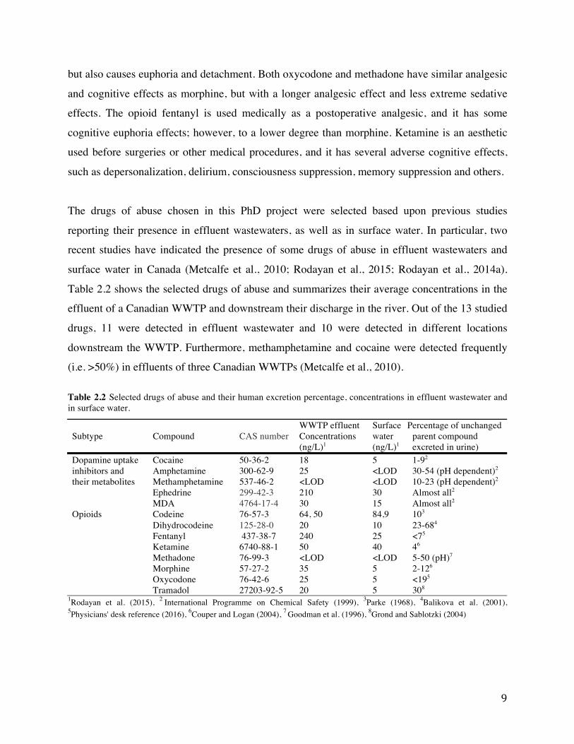
but also causes euphoria and detachment. Both oxycodone and methadone have similar analgesic and cognitive effects as morphine, but with a longer analgesic effect and less extreme sedative effects. The opioid fentanyl is used medically as a postoperative analgesic, and it has some cognitive euphoria effects; however, to a lower degree than morphine. Ketamine is an aesthetic used before surgeries or other medical procedures, and it has several adverse cognitive effects, such as depersonalization, delirium, consciousness suppression, memory suppression and others. The drugs of abuse chosen in this PhD project were selected based upon previous studies reporting their presence in effluent wastewaters, as well as in surface water. In particular, two recent studies have indicated the presence of some drugs of abuse in effluent wastewaters and surface water in Canada (Metcalfe et al., 2010; Rodayan et al., 2015; Rodayan et al., 2014a). Table 2.2 shows the selected drugs of abuse and summarizes their average concentrations in the effluent of a Canadian WWTP and downstream their discharge in the river. Out of the 13 studied drugs, 11 were detected in effluent wastewater and 10 were detected in different locations downstream the WWTP. Furthermore, methamphetamine and cocaine were detected frequently (i.e. >50%) in effluents of three Canadian WWTPs (Metcalfe et al., 2010).

Table 2.2 Selected drugs of abuse and their human excretion percentage, concentrations in effluent wastewater and in surface water.

Subtype Compound CAS number WWTP effluent Concentrations (ng/L)1

Surface water (ng/L)1

Percentage of unchanged parent compound excreted in urine)

Dopamine uptake inhibitors and their metabolites

Cocaine 50-36-2 18 5 1-92 Amphetamine 300-62-9 25 <LOD 30-54 (pH dependent)2 Methamphetamine 537-46-2 <LOD <LOD 10-23 (pH dependent)2 Ephedrine 299-42-3 210 30 Almost all2 MDA 4764-17-4 30 15 Almost all2

Opioids Codeine 76-57-3 64, 50 84,9 103 Dihydrocodeine 125-28-0 20 10 23-684 Fentanyl 437-38-7 240 25 <75 Ketamine 6740-88-1 50 40 46 Methadone 76-99-3 <LOD <LOD 5-50 (pH)7 Morphine 57-27-2 35 5 2-126 Oxycodone 76-42-6 25 5 <195 Tramadol 27203-92-5 20 5 308

1Rodayan et al. (2015), 2 International Programme on Chemical Safety (1999), 3Parke (1968), 4Balikova et al. (2001), 5Physicians' desk reference (2016), 6Couper and Logan (2004), 7 Goodman et al. (1996), 8Grond and Sablotzki (2004)

Cocaine (MW: 303.36, pKa: 8.61, Log Kow: 2.3)

Amphetamine (MW: 135.21, pKa: 10.1, Log Kow: 1.76)

Methamphetamine (MW: 149.2, pKa: 10.21, Log Kow: 2.07),

Ephedrine (MW: 165.23, pKa: 9.65, Log Kow: 1.13),

MDA (MW:179.22, pKa: 9.67, Log Kow: 1.64)

Dihydrocodeine (MW:301.38, pKa: 8.8, Log Kow: 1.49)

Fentanyl (MW:336.47, pKa: 8.6, Log Kow: 4.05)

Ketamine (MW:237.73, pKa: 7.5, Log Kow: 2.18)

Methadone (MW:309.4, pKa: 8.94, Log Kow: 3.93)

Morphine (MW:285.34, pKa: 9.85, Log Kow: 0.89)

Oxycodone (MW:315.37, pKa: 8.28, Log Kow: 0.66)

Tramadol (MW:263.37, pKa: 9.41, Log Kow: 2.63)

Figure 2.3 Chemical structure, molecular weight (MW, g/mol) and properties of the studied drugs of abuse. pKa and Log Kow values obtained from National Center for Biotechnology Information (2004) N.A.:unavailable data.

Regarding the metabolism of drugs of abuse, only 1-9% of an ingested dose of cocaine is excreted as the parent compound, and the remaining dose is excreted as benzoylecgonine (35-54%) and ecgonine methyl ester (32-49%) (Baselt, 1984). Benzoylecgonine, the main metabolite of cocaine, has been detected in all samples (n=36) collected from effluents of three WWTPs in Canada (Metcalfe et al., 2010) at concentrations of 62-775 ng/L, and was added to this study to account for its removal in the treatment train. In fact, benzoylecgonine concentrations were 3-5 times higher than those of cocaine in several studies, as summarized in a review article by Ratola et al. (2012). On the other, hand a higher portion of the ingested dose is excreted unchanged for amphetamine-type drugs (i.e. MDA, ephedrine, amphetamine and methamphetamine) from the human body, making it not as crucial to also monitor the fate of the metabolites (Baselt, 2000; Zuccato et al., 2008). Only a small portion of the intake opioids are excreted unchanged from the human body. However, the main human metabolite of methadone, EDDP, was included in this study, due to its relatively high concentrations observed in the effluent of a WWTP in Canada (110 ng/L) (Rodayan et al., 2015), while methadone itself was not detected in the same study. In other studies, the concentration of EDDP in influent wastewater was found to be more than twice the concentration of methadone (Baker et al., 2012; Castiglioni et al., 2006b). Codeine is partially metabolized in the human body to morphine that is also a synthesized opioid included in this study (International Programme on Chemical Safety, 1999).

Benzoylecgonine (MW: 252.27 pKa: N.A., Log Kow: -1.32)

EDDP (2-ethylidene-1,5-dimethyl-3,3- diphenylpyrrolidine)

(MW: 270.28 pKa: 9.64, Log Kow: 4.94)

Figure 2.4 Chemical structure, molecular weight (MW, g/mol) and properties of the studied metabolite of cocaine (benzoylecgonine) and methadone (EDDP). pKa and Log Kow values obtained from National Center for Biotechnology Information (2004). N.A.:unavailable data.

2.2.3. Hormones

The two hormones monitored in this project are androstenedione and estrone. Androstenedione is a natural androgenic steroid produced in the human body by the adrenal glands, testicles and ovaries and used to produce estrogens and testesterone. Androstenedione is also used to produce tablets or sprays that are used by athletes, mostly illegally, to increase the testosterone level in

the blood (Murray, 2002). Due to the limited literature investigating its fate during wastewater treatment (Esperanza et al., 2007), it was selected as a model androgen for this project. Estrone is also a natural hormone excreted by the ovaries. Estrone was found to be present in the influent to 18 municipal WWTPs at concentrations of 19–78 ng/L and in the effluent at concentrations of 1–96 ng/L (Servos et al., 2005). Figure 2.5 summarizes the main properties of these two hormones.

Estrone (MW: 270.366 pKa: 10.3, Log Kow: 3.13)

Androstenedione (MW: 286.41 pKa: N.A., Log Kow: 2.75)

Figure 2.5 Chemical structure, molecular weight (MW, g/mol) and chemical properties of estrone and androstenedione. pKa and Log Kow values obtained from National Center for Biotechnology Information (2004). N.A.:unavailable data.

2.2.4. Other target contaminants

Three other emerging contaminants that belong to different categories, namely sucralose, caffeine and triclosan were selected for this project. Sucralose is a non-nutritive artificial sweetener, mostly known as Splenda. It has been widely detected in 19 drinking water systems in the USA at concentrations of 47-2900 ng/L and 49-2400 ng/L in the source water and in the finished water, respectively and has been proposed as a tracer of wastewater contamination (Mawhinney et al., 2011). Caffeine is a widely-used central nervous stimulant found in beverages, such as coffee and tea and in some foods, such as chocolate. Caffeine was identified to be one of the potential indicator compounds of wastewater treatment efficiency and the contamination of surface water by wastewater, according to the previously discussed criteria (Dickenson et al., 2011). Triclosan is a common antiseptic agent found in household products and personal care products, such as toothpastes, soaps, detergents and many others. It was selected since it was observed to resist conventional wastewater treatment resulting in its discharge to the environment (Ricart et al., 2010). The main properties of these three compounds are presented in Figure 2.6.

Sucralose (MW: 397.64, pKa: 11.8, Log Kow: -1)

Triclosan (MW: 289.54, pKa: 7.9, Log Kow: 4.76)

Caffeine (MW: 194.19, pKa: 14, Log Kow: -0.07)

Figure 2.6 Chemical structure, molecular weight (MW, g/mol) and chemical properties of sucralose, caffeine and triclosan. pKa and Log Kow values obtained from National Center for Biotechnology Information (2004), except for sucralose (Busetti et al., 2015; Subedi & Kannan, 2014a). N.A.:unavailable data.

2.3. Fate in WWTPs

It has been determined long ago that the main route of PPCPs in the environment are discharges from wastewater treatment plants (WWTPs) (Ternes et al., 2004b). WWTPs provide primary, secondary and, in some cases, tertiary (advanced) treatment through biological, physical and chemical processes. The most widely-used technology for biological treatment across the world is the activated sludge process (World Bank Group, 2016). WWTPs are designed to meet regulations on suspended matter, as well as other total organic matter and nutrients but are not specifically designed to treat CECs, considering the absence of regulations governing their discharge. Nevertheless, along with the removal of the traditional pollutants, some removal of the CECs was reported to take place in WWTPs, as summarize in the following sections.

2.3.1. CEC removal mechanisms

According to Rogers (1996), several processes are involved in the elimination of CECs from wastewater during treatment. These include degradation (biological and abiotic), as well as the two physical processes: volatilization and sorption to sludge. Sorption occurs when a portion of the CEC gets bound to the suspended solids and subsequently settles with the sludge (Ternes et al., 2004b). Adsorption can take place due to one of the following interactions (Jelic et al., 2012; Meakins et al., 1994; Ternes et al., 2004b):

1- Interaction between the hydrophobic groups of the CEC (i.e. aliphatic or aromatic groups) with the lipophilic cell membrane of the microorganisms or the fat contained in the sludge

2- Electrostatic reactions between the positively charged groups of the CEC and the negatively charged surfaces of the microorganism

3- Other interactions: hydrogen bonding, ionic interactions and surface complexation

Due to the different processes that affect the sorption behaviour (Jelic et al., 2012), the extent of adsorption is influenced by a number of conditions and factors, including the treatment conditions and the physico-chemical properties of the CEC. A high log Kow (>4) is associated with higher hydrophobicity and more adsorption to sludge through hydrophobic interactions (Thompson et al., 2011). Not only log Kow of the CEC influences its adsorption, but also its acidic dissociation constant (pKa). When the pKa of the CEC has a value that is closer to or higher than the pH of the wastewater, the potential of the CEC to dissociate and occur in the soluble phase decreases, increasing, therefore, its potential to get attached to particulate matter (Thomas & Foster, 2005; Yang et al., 2011). A combination of high log Kow and high pKa provides suitable conditions for adsorption (Yang et al., 2011). For instance, naproxen and ibuprofen having relatively high log Kow (i.e. >3, Figure 2.1), do not tend to highly adsorb to sludge due to their pKa (i.e. <5, Figure 2.1) that is much lower than the typical pH of wastewater (i.e. 6.5-8.5) implying their presence mainly as ions in the aqueous phase (Thomas & Foster, 2005). Biological degradation (biodegradation), which involves the consumption of organic

contaminants by biological means, has been reported in literature as the main mechanism of removal for many CECs included in this study. Due to their low concentrations in wastewater (in the range of ng/L to μg/L), however, the microorganisms do not use the CECs in wastewater as a main carbon source (Heberer, 2002a; Ternes, 1998). That is, the CECs get biodegraded with and in the presence of another substrate that constitutes the primary substrate: A process that is known as co-metabolism (Ternes et al., 2004b). A higher sludge age, achieved by a higher solids retention time (SRT), was observed to increase the biodegradation of the CECs (Blair et al., 2013b; Buser et al., 1998). This is either due to a higher diversity in the population of the microorganisms in the aged sludge or to the higher diversity of the metabolic activity in response

to a decreasing amount of substrate with time, as explained by Ternes (1998). The existence of nitrifying microorganisms was found to enhance the removal of CECs, due to their enhanced capability to co-metabolise compared to other types of microorganism (Luo et al., 2014). However, a poor correlation was sometimes obtained between the SRT and the CEC removals and linked to the SRT variations at a low range (Santos et al., 2009), indicating that the effect of SRT on CEC removals is not linear and depends on the targeted range. Higher HRT was often linked to higher CEC removals and interpreted by the availability of more time for CECs with slow kinetics to biodegrade or adsorb (Fernandez-Fontaina et al., 2012; Santos et al., 2009). Temperature also plays an important role in influencing the CEC removal processes due to its effect on microbial growth and activity (Hai et al., 2011; Luo et al., 2014). Volatilization is a physical process involving the transfer of CECs from the surface of wastewater to the air. According to Stenstrom et al. (1989), the tendency of CECs to undergo volatilization is assessed empirically using the air-water partition coefficient (dimensionless Henry’s Law constant, Hc) and its relation to the Kow. Volatilization is deemed significant if Hc>10-4 and Hc/Kow>10-9 (Rogers, 1996; Stenstrom et al., 1989). The target CECs are large molecules with low Henry’s constants and are not expected to be significantly removed by volatilization (Struijs et al., 1991; Virkutyte et al., 2010). Abiotic degradation of CECs includes means of degradation that are not biological, such as hydrolysis and photolysis. Hydrolysis in domestic wastewater is slower than other processes and is, therefore, often considered negligible (Schwarzenbach et al., 1993). Pharmaceuticals and drugs are designed for oral intake, which explains their low tendency to chemically degrade in water (Andreozzi et al., 2003). Except for lagoon WWTPs, photolysis under sunlight conditions is also not likely to contribute significantly to the removal of CECs in WWTPs, due to the low exposure to light in the highly-turbid bioreactor, as well as the generally long half life of the photolysis process in comparison to the short retention times of conventional treatment steps (Daneshvar et al., 2010; Deegan et al., 2011; Lishman et al., 2006).

2.3.2. Overall removal of CECs in WWTPs

Table 2.3 shows the range of concentrations observed for CECs in untreated wastewater worldwide. The concentrations of CECs in wastewater are highly variable, depending on the type

of the wastewater and the country (Ratola et al., 2012). The majority of the investigated CECs have concentrations in the ng/L range in wastewater, while few of them, namely ibuprofen, sucralose and caffeine, have concentrations higher than 1 μg/L. Data for the occurrence of drugs of abuse in wastewater and their removal in WWTPs is much more limited than for the other CECs on the list, such as pharmaceuticals and hormones. Several studies reported the overall efficiency of WWTPs at treating CECs, as also summarized in Table 2.3.

Table 2.3 Concentrations of the target CECs in influent wastewater to WWTPs and the range of their overall removal efficiencies in WWTPs as reported by several past studies carried out in different countries.

Type and Subtype References Compound Influent Concentration (ng/L) Removal (%)

Antibiotics

1-11 Trimethoprim 60–6,800 <0–81.6 Sulfamethoxazole <3–980 4–88.9 Acetaminophen 1,570–56,900 98.7–100

Anti-inflammatory

Codeine 1732–32,295 13-40 1,3,4,5,7,9,11,12,13,14,20,42 Ibuprofen <4–603,000 72–100 Naproxen <2–52,900 43.3–98.6

Antiepileptic

1,2,4,5,7,9,10,11 Carbamazepine <40–3,780 <0–62.3 Dopamine uptake inhibitors and their metabolites

15-35,42,51 Cocaine 4-4700 90–100 Benzoylecgonine 9-7500 85–95 Amphetamine ˂LOD–5,236 9–100 Methamphetamine ˂LOD–800 0–99 Ephedrine 100-429 34–88 MDA ˂LOD–1,690 60

Opioids 15,16,17,18,20,21,22,23,36,37,38,40,41,42

Dihydrocodeine ˂LOQ–16 - Fentanyl - - Ketamine 7–50 35–84 Methadone 3.4–1,531 9–22 EDDP 8–33 Morphine ˂LOQ–929 26–98 Oxycodone 70–500 28 Tramadol 8508–89,026 35–37

Hormones 1,14,43,44,45 Androstenedione 74–87 100 Estrone 0.01–0.07 75–91

Others 1,2,5,7,10,11,12,13 Caffeine 220,000–290,000 50–100 46,47,48,49 Sucralose 1,700–33,000 <0–45 1,5,6,7,45,46 Triclosan 0.03–24 71–99

1: Behera et al. (2011); 2: Choi et al. (2008); 3: Gracia-Lor et al. (2012); 4: Kasprzyk-Hordern et al. (2009); 5: Loos et al. (2013); 6:Martin Ruel et al. (2010); 7:Santos et al. (2009); 8:Stamatis and Konstantinou (2013); 9:Terzic et al. (2008); 10:Zhou and Oleszkiewicz (2010); 11: Singer et al. (2010); 12:Stamatis et al. (2010); 13: Yu and Chu (2009); 14:Zorita et al. (2009); 15: Berset et al. (2010); 16:Bijlsma et al. (2012); 17:Castiglioni et al. (2006b); 18:Huerta-Fontela et al. (2008); 19: Kasprzyk-Hordern et al. (2008a); 20:Kasprzyk-Hordern et al. (2009); 21:Postigo et al. (2010); 22: Terzic et al. (2010); 23:Van Nuijs et al. (2011); 24:Yargeau et al. (2014b); 25:Metcalfe et al. (2010); 26:Loganathan et al. (2009); 27:Bones et al. (2007); 28:Gheorghe et al. (2008); 29: González-Mariño et al. (2010); 30:Hummel et al. (2006); 31:Karolak et al. (2010); 32:Kasprzyk-Hordern et al. (2008b); 33:Van Nuijs et al. (2009a); 34:Van Nuijs et al. (2009b); 35:Zuccato et al. (2005); 36:Boleda et al. (2009); 37:Martínez Bueno et al. (2009); 38:González-Mariño et al. (2012); 39:Huerta-Fontela et al. (2008); 40:Van Nuijs et al. (2009c); 41:Pedrouzo et al. (2011); 42:Rodayan et al. (2014a); 43:Janex-Habibi et al. (2009); 44:Nie et al. (2012); 45:Esperanza et al. (2007); 46:Brorström-Lunden (2008b); 47:Pasquini et al. (2013); 48:Rodayan et al. (2015); 49:Subedi and Kannan (2014a); 50:Kumar et al. (2010); 46:Pothitou and Voutsa (2008); 51:Boles and Wells (2010)

As shown in Table 2.3, while some compounds have high removals (up to 100%), others are persistent (i.e. carbamazepine, codeine, methadone and others). The removals in Table 2.3 also varied for each compound among the different studies due to the differences in the treatment trains, operating conditions and other conditions. This highlights the importance of further understanding the removal process of CECs during wastewater treatment in order to be able to predict their removal and improve their removal in WWTPs. Although these overall removals of CECs convey an important message on the efficiency of the existing WWTPs at removing CECs, they do not distinguish between the efficiency of the different treatment steps, limiting as well the understanding of the contribution of different removal mechanisms.

2.3.3. CEC removal per treatment step

Although there is abundant literature on the overall efficiency of WWTPs at removing CECs (Table 2.3), fewer studies looked at the efficacy of each treatment step separately. Evaluating the individual efficiencies is essential for determining the contribution of distinct processes playing a role in the removal and, eventually, optimizing and designing efficient treatment steps. For instance, Carballa et al. (2005) suggested that evaluating the removals of the primary treatment could provide important information for the optimization of the removal of CECs in primary settlers. Enhancing the CEC removal in primary settlers could minimize the cost of upgrading secondary and tertiary steps (Carballa et al., 2005) and is generally overlooked. Furthermore, obtaining CEC data per treatment step is essential for the calibration of fate models of CECs that provide a valuable and cost-effective tool for predicting the fate of CECs in different treatment systems.

2.3.3.1. Primary settling and activated sludge Table 2.4 summarizes results from previous studies that investigated the removal of the studied CECs in primary settlers and activated sludge treatment, separately. Primary treatment by primary settling concentrates and removes settleable organics from the wastewater. Typically, primary settlers remove 25 to 35% of the biological oxygen demand (BOD) and 40% to 60% of the total suspended solids (TSS) (Office of Water Programs, 1980). However, poor removal of CECs (<50%) was observed in primary settler for most of the CECs included in the list of this project, as shown in Table 2.4. This could be due to the low tendency to adsorb onto primary

sludge that subsequently settles in the clarifier. The low affinity of a contaminant to primary sludge can be explained by its low hydrophobicity manifested by a low log Kow or a high pKa (Figure 2.1-2.6) (Behera et al., 2011). Owing to its hydrophobic nature (Winkler et al., 2007), triclosan was shown to have a positive removal during primary treatment in different studies (Table 2.4), suggesting its high adsorption on the fat-rich primary sludge. It was previously demonstrated that coagulant additives, such as ferric chloride (FeCl3) and aluminum sulfate (Al2(SO4)3) frequently added for enhanced particulate and/or phosphorus precipitation, could improve the removal of some pharmaceuticals, such as naproxen during primary clarification (Clara et al., 2005b). Biological treatment removes BOD at higher levels than primary treatment (Spellman, 2007). Prior to 1950, activated sludge processes were designed to remove only the BOD, after which further developments in their configuration and additives were introduced to achieve nitrogen and phosphorus removal (Ternes et al., 2004b). However, activated sludge units are still not designed for the removal of CECs, also referred to as micropollutants (MPs). Unlike primary treatment, activated sludge units, for which more CEC removal studies are available, removed up to 100% of the incoming load for some of the CECs (Table 2.4). The high variations between the efficacy of the different activated sludge systems investigated in different studies could be attributed to the different operating conditions that significantly impact the biodegradation process of CECs. Other factors causing the variations could be related to the monitoring techniques, which will be discussed later in Section 2.4. In some cases, studies reported the CEC removal as a range, due to the fact that different operating conditions, mainly SRT, were investigated. As shown in the Table 2.4, some CECs, in particular carbamazepine and sucralose seem to be of recalcitrant nature during biological treatment, as reported by several studies. By contrast, ibuprofen, naproxen, benzoylecgonine, acetaminophen and caffeine exhibit consistently high removals from the aqueous phase during activated sludge treatment. Most of the studies listed in Table 2.4 did not distinguish between different mechanisms contributing to elimination of CECs from the aqueous phase (i.e. biodegradation and sorption) due to the unavailability of data concerning the CEC load sorbed onto sludge.

Table 2.4 Removal of CECs obtained in different activated sludge units and primary clarifiers, evaluated separately. Compound Primary clarifier (%) References Activated sludge (%) References Trimethoprim 15 3 70; 40; 7; -30; 53 3; 19; 5; 16; 17 Sulfamethoxazole -10 2 65; 56; -138–60; 90; 70; 54;

74; 42 2; 7; 5; 6; 3; 18; 16; 5; 20

Acetaminophen 0; 22 3; 4 86; 99.9 7; 16 Codeine 4 12 45; 9 6; 12 Ibuprofen -7; 5; 88 2; 3; 4 75; 70; 83; 90; 100; 99; 98 8; 2; 7; 6; 3; 19; 20 Naproxen 3; -10; <0 2; 3; 4 78; 45; 85; 80; 90; 72 8; 2; 7; 6; 3; 19 Carbamazepine 26; -10 14; 3 <10; -20; 25; <10; -11– -43 7; 6; 3; 16; 20 Gemfirozil 0 3 39; 5 7; 16 Cocaine 70; 0 11; 12 90; 40 12; 11 Benzoylecgonine 50; 2 11; 12 83; 40 12; 11 Amphetamine 60; 5 11; 12 40 11 Methamphetamine -120; 3 11; 12 79; -20 12; 11 Ephedrine 9 12 25 12 Dihydrocodeine - - 50 13 Fentanyl - - - - Ketamine - - - - Methadone 14; -110 11; 12 -5 11 EDDP -40; 0 11; 12 26 12 Morphine 0; 5; 25 3; 11; 12 95 13 Oxycodone -4 12 28 12 Tramadol 21 12 35 6 Androstenedione -8 1 <100 1 Estrone 40; - 8; -59 2; 3; 4 40; -49–99; -40–20; 70; 85 2; 15; 5; 6; 3 Caffeine 17 3 100 3 Sucralose - - -40–10 10 Triclosan 53; 32 9; 4 75 3 1: Esperanza et al. (2007); 2: Carballa et al. (2004); 3: Behera et al. (2011); 4: Blair et al. (2013b); 5: Göbel et al. (2007); 6: Kasprzyk-Hordern et al. (2009); 7: Radjenović et al. (2007); 8: Stumpf et al. (1999); 9: Winkler et al. (2007), 10: Brorström-Lunden (2008a),11: Subedi and Kannan (2014b), 12: Rodayan et al. (2014a), 13: Wick et al. (2009); 14: Zhou et al. (2009); 15: Joss et al. (2004); 16:Lindberg et al. (2006); 17:Batt et al. (2006); 18:García-Galán et al. (2011); 19:Radjenović et al. (2009b); 20: Clara et al. (2005b)

Tertiary treatment is an optional final polishing step for wastewater before discharge into the environment. Tertiary treatment units are added mostly in order to meet regulations with regards to traditional pollutants discharge and are often associated with a higher cost. Different forms of tertiary treatment for wastewater exist, such as sand filtration, membrane filtration and granular activated carbon (GAC). Disinfection is also implemented for the effluent wastewaters in order to reduce the amount of microorganisms in the discharged effluent. The main disinfection method is chlorination. Other disinfection processes implemented include ozone (O3) and ultraviolet (UV) disinfection. Tertiary treatment provides extra removal of CECs that are persistent during biological secondary treatment. The capacity of membrane tertiary processes

(micro- and ultrafiltration), as well as UV and ozone disinfection processes at treating CECs has been evaluated in several pilot- and full-scale studies (De la Cruz et al., 2012; Gerrity et al., 2011; Hernández-Leal et al., 2011; Jermann et al., 2009; Röhricht et al., 2009; Sui et al., 2010; Yangali-Quintanilla et al., 2011), but these technologies are not investigated in this PhD project. The two tertiary treatment steps evaluated in this project are rotating biological contactors and sand filtration. The rotating biological contactors technology (RBCs) was first developed in Germany in the 1960s. Although rotating biological contactors (RBCs) are often used as the main biological treatment step considered as secondary treatment, they could be coupled to activated sludge units as a tertiary step for the reduction of BOD5 and nitrogen. In RBCs, the biomass growth is attached to rotating discs, compared to the suspended biomass in activated sludge units. Attached growth processes are known for their simple operation and higher energy efficiency, and by 2007, around 600 RBCs plants were implemented in the US for the treatment of wastewater (Water Environment Federation, 2008). A small number of studies investigated the removal of our target CECs by full-scale RBCs (Batt et al., 2007; Gabet-Giraud et al., 2010; Kanda et al., 2003; Simonich et al., 2002; Thompson et al., 2005) and another study examined bench-scale RBCs (Vasiliadou et al., 2014). Vasiliadou et al. (2014) reported that caffeine had high removal in RBCs that ranged from 39% to 100%, with the higher removals being linked to higher HRT. Batt et al. (2007) observed reduction in concentration of sulfamethoxazole and trimethoprim of 36% and 75%, respectively in full-scale RBCs with HRT of 4 h. The removal of triclosan by RBCs was reported to be 25-30% by Thompson et al. (2005). In all of the aforementioned studies, RBCs were used as a secondary treatment process. Tertiary sand filtration provides a simple and cost-effective means for the reduction of TSS and ammonia in secondary effluents to meet stringent regulations as it operates by retaining particulate matter. The performance of sand filters in terms of removing CECs was previously examined, and they were found to have variable efficiencies, depending on the compound and the operating conditions (Gao et al., 2012; Göbel et al., 2007; Matamoros et al., 2007; Nakada et al., 2007; Zorita et al., 2009). The pain-killers ibuprofen and naproxen were monitored in sand filters, and removals of naproxen were found to range from negative values to 50% at different

seasons (HRT=0.5 h) by Nakada et al. (2007), while no removal was observed by Zorita et al. (2009) (HRT=1 h). Ibuprofen, on the other hand, had removal ranging 20-100% in the same studies (Nakada et al., 2007; Zorita et al., 2009). Nakada et al. (2007) also observed that estrone had variable removals in a sand filter (i.e. <0 – 60%), depending on the season and that triclosan was poorly removed (i.e. <50%). Carbamazepine was also observed to have poor removals (i.e. <15% with some negative removals) by sand filtration in multiple studies (Gao et al., 2012; Nakada et al., 2007; Sui et al., 2010). Considerable removal (over 60%) of trimethoprim was observed previously (Nakada et al., 2007; Sui et al., 2010), while Göbel et al. (2007) reported variable removal efficiencies (i.e. 15-74%) of trimethoprim in sand filters of different WWTPs. Sand filtration was also reported to remove 19% of the incoming sulfamethoxazole by Gao et al. (2012) and around 30% by Nakada et al. (2007), whereas Göbel et al. (2007) reported insignificant change in the loads of sulfamethoxazole when passed by sand filtration. Nakada et al. (2007) attributed the observed poor removal of CECs by sand filtration to their hydrophilic nature (manifested by a low log Kow) and observed that a combination of ozonation and sand filtration enhances the system’s removal of CECs. Removal in sand filters is attributed to adsorption to solid particles that are retained by the sand filter. However, previous studies also indicated that biodegradation can contribute to CEC removal due to the formation of biofilm on sand particles (Göbel et al., 2007).

2.4. Hydraulics and sampling techniques

It was previously suggested that the transport of the CECs in treatment steps is highly affected by the hydrodynamics of the treatment unit (Majewsky et al., 2011; Ort et al., 2010). Hence, a measured difference in the micropollutant load between the sampled inlet and the outlet of a full-scale treatment unit is not necessarily due to removal. It could simply mean that the incoming contaminant load has not yet reached the outlet by the time the sample was collected due to the hydraulic delay. This could result in a mismatch of measured influent and effluent loads that are used to calculate removal efficiencies. Most of the studies investigating the CEC overall removal in WWTPs and the removal per treatment step (results in Table 2.3 and Table 2.4, respectively) did not adequately account for the hydraulics of the WWTP in the removal calculations. In a review paper, Petrie et al. (2015) argued that sampling is fundamentally the most important step

in obtaining high quality data on CEC but still one of the most overlooked aspects. Ort et al. (2010) showed that of 87 peer-reviewed articles examining CEC fate in WWTPs, only 10% provided justification for the sampling strategy used. Negative removals and variable removal levels compiled in Table 2.4 could be attributed to the overlooking of the hydrodynamics factor for sampling and removal calculation.

2.4.1. Composite vs grab samples

Collecting grab samples was deemed to overlook the temporal variations in concentrations. Compared to 24-h composite samples, grab samples ignore the diurnal variation in the contaminant loads that generally peaks at 7:00-9:00 and influences the match between the sampled inlet and outlets samples (Petrie et al., 2015). Hence, 24-h composite samples provide a more representative overview of the load that enters at a certain time. Table 2.5 shows the sampling technique used by the studies that investigated the CEC removal in primary and secondary treatments, separately. It could be observed from Table 2.5 that the implementation of the 24-h composite sampling strategy is becoming widespread.

2.4.2. Time-proportional vs flow proportional and frequency of sampling

Ort et al. (2010) emphasized the need for collecting flow-proportional samples in order to avoid bias of sampling due to the flow variations and showed that only 23% of 83 peer-reviewed articles on CEC removal described their collected samples as flow-proportional. This could be attributed to the generally more complex sampling instruments required for flow-proportional samples. From Table 2.4, out of the 11 studies reporting removal per treatment step, three studies collected time-proportional samples, while eight studies collected flow-proportional samples, and one study collected both types of samples. The frequency of the sample collection was also suggested to play an important role in the quality of the sample and the degree it represents reality. In a proposed sampling guide, Ort et al. (2010) established rules of thumbs to estimate the minimum required frequency of the sampling in order to obtain representative samples, depending on the target CECs and their consumption information. In general, higher frequency is associated with a higher resolution of the sampling; hence, continuous sampling was claimed to be the ideal precautionary sampling mode (Ort et al., 2010). However, several issues arise when implementing continuous sampling, in particular with regards to the sampler tubes that are normally purged from one time to another to avoid clogging, as well as storage capacity issues;

hence, only 1% of 83 reviewed articles used continuous sampling (Ort et al., 2010). Therefore, a compromise needs to be established between the operational feasibility and the high frequency of sampling.

2.4.3. HRT and RTD

As seen in Table 2.5, three out of 11 of the studies lagged their effluent sampling by a time period equivalent to the HRT of the treatment unit investigated to account for the retention time. Petrie et al. (2015) suggested that the approach of temporally shifting the effluent sampling by the HRT is impractical for systems with a higher HRT, such as activated sludge (normally HRT >6). In fact, accounting for the HRT solely assumes plug flow characteristic, which is not necessarily the case in units with a high degree of mixing. Hence, not only accounting for the HRT is essential in CEC fate studies but also taking into consideration the unequal distribution of residence time between fluid elements due to mixing, as suggested by Majewsky et al. (2011). To reduce the measurement uncertainty due to short sampling periods that do not account for the residence time distribution (RTD), prolonged sampling campaigns are required to cover most of incoming contaminant load, which often implies higher cost for sampling and analysis. An approach combining prior hydraulic modelling and defined sampling strategy was developed by Majewsky et al. (2011) to account for the distribution of the residence time in CEC fate studies and that aims at achieving a compromise between cost minimization and error reduction by the determination of the necessary number of sampling days. Once the hydraulic model of the treatment unit has been defined (further discussed in section 2.7.1), it can be used to obtain load fractions of the influent that describe the load exiting on a specific day. These fractions are used to calculate a hypothetical output load that would leave the treatment unit on a specific day in the case of no biodegradation as fractions of input contaminant load of each previous day (also called fractionated load), as illustrated in Figure 2.7. For example, on the fourth day of sampling the effluent in Figure 2.7 contains 64% of the CEC load entering on the same day, 31% of the load entering the previous day and 0.7% of the load entering two days ago, assuming no biodegradation. Comparing this load with the actual effluent loads gives a reliable insight of the contaminant load lost in the system due to biodegradation without the bias of hydraulic effect. In only one study in Table 2.4 this method was applied to account for RTD in calculating CEC removals in activated sludge (Rodayan et al., 2014a).

Obtaining reliable measured data on the fate of CECs is essential for the calibration of mathematical models describing their fate, as emphasized by Ort et al. (2010). Alternative sampling techniques, not discussed above, include passive sampling techniques that have several shortcomings, and developments are still needed to investigate the uptake of CECs by passive samplers (Mills et al., 2014). Passive sampling techniques; however, are not used in this thesis.

Table 2.5 Sampling techniques used for the studies shown in Table 2.4, including the type of sample (grab or 24-h composite, flow-proportional or time-proportional), the consideration of residence time distribution (RTD) or hydraulic residence time (HRT) and the inclusion of sludge samples in the analysis. Studies on CEC removals in primary, secondary, separately

Grab or composite

Flow- or time- proportional

RTD/ HRT considered

Sludge collected

Esperanza et al. (2007) N.A N.A. No Yes Carballa et al. (2004) 24-h Time HRT No Behera et al. (2011) Grab - No No Blair et al. (2013b) 24-h Flow and Time No No Göbel et al. (2007) 24-h Flow No Yes Kasprzyk-Hordern et al. (2009) 24-h and grab N.A. No No Radjenović et al. (2007) 24-h Time HRT No Stumpf et al. (1999) 24-h N.A. No No Winkler et al. (2007) N.A. N.A. N.A. Yes Brorström-Lunden (2008a) 24-h Flow Yes No Subedi and Kannan (2014b) 24-h N.A. No Yes Rodayan et al. (2014a) 24-h Flow RTD No Wick et al. (2009) 24-h N.A. HRT Yes Zhou et al. (2009) N.A. N.A. N.A. No Joss et al. (2004) 24-h Flow No NoLindberg et al. (2006) 24-h Flow No Yes Batt et al. (2006) 24-h Flow No No García-Galán et al. (2011) 24-h Flow No No Radjenović et al. (2009b) 24-h Flow No Yes Clara et al. (2005b) 24-h Time No No

Figure 2.7 Illustration of the concept of the residence time distribution and its impact on sampling strategies.

Eff

luen

t co

ntam

inan

t co

ncen

trat

ion

Infl

uent

co

ntam

inan

t co

ncen

trat

ion

Time (days)

64%

31%

0.7%

Day 1 Day 2 Day 3 Day 4

2.5. Fate pathways

2.5.1. Sludge and values

The majority of studies investigated the fate of CECs by analyzing aqueous samples from the input and the output of units and overlooking the contaminant load that might be sorbed onto suspended particulate matter in the streams. In 2009, Miège et al. (2009) reviewed 117 peer-reviewed articles examining CEC fate in WWTPs and found that only 15 of these reported CEC concentrations in sludge and only one considered the CEC concentration in both aqueous and particulate phase for removal calculations. Table 2.4 and Table 2.5 also confirm that most of the studies analyzing CEC removal per treatment steps did not consider the sludge samples. Petrie et al. (2015) attributed the scarcity of studies considering CEC loads in biosolids to the fact that it is experimentally demanding to analyze for CECs in biosolids. This is due to the large sample volumes required and the multiple extraction methods involved (Baker & Kasprzyk-Hordern, 2011; Edwards et al., 2009; Radjenović et al., 2009a).

As discussed earlier, adsorption is one important fate pathway of some CECs during treatment.

Ignoring the adsorption behaviour of CECs when investigating their removal in WWTPs leads to

bias due to a number of factors. Firstly, the concentrations of pharmaceuticals in the particulate

matter could be of significance and have values as high as 26-296 ng/L (Petrie et al., 2014). In

the same study by Petrie et al. (2014), it was found that triclosan load within the suspended

matter in the secondary effluent comprised >20% of its total load, despite the low total

suspended solids (TSS) concentration in that stream. Hence, calculations of CEC removal using

loads based solely on the aqueous phase could lead to erroneous results. This is explained by the

fact that the CEC removal from the aqueous phase does not necessarily indicate the CEC was

transformed and will not be discharged into the environment, but it could also suggest that the

CEC was transported to the particulate compartment. Hence, ignoring the potential transfer of

CECs to sludge might result in underestimation of the risk of discharge and reuse of this residue

of WWTPs. Before discharge, the generated sludge is treated, after which it is often used for

agricultural purposes. To date, there is no legislation controlling the CEC concentrations in

treated sludge that is applied to agricultural lands (Petrie et al., 2015). In fact, triclosan was

shown to persist in biosolids-amended soils for up to eight months at concentrations of 800-1000

ng/g, after which its transformation product methyl-triclosan is formed and was detected (Butler

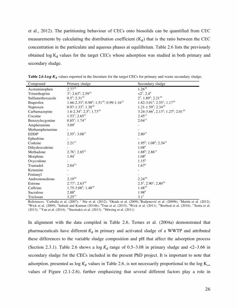
et al., 2012). The partitioning behaviour of CECs onto biosolids can be quantified from CEC

measurements by calculating the distribution coefficient ( ) that is the ratio between the CEC

concentration in the particulate and aqueous phases at equilibrium. Table 2.6 lists the previously

obtained log values for the target CECs whose adsorption was studied in both primary and

secondary sludge.

Table 2.6 values reported in the literature for the target CECs for primary and waste secondary sludge. Compound Primary sludge Secondary sludge Acetaminophen 2.7710 1.2610 Trimethoprim 33; 2.634; 2.5914 <23, 2.44 Sulfamethoxazole 0.54; 2.3110 23, 1.894; 2.2110 Ibuprofen 1.66-2.335; 0.984; 1.5110; 0.99-1.1612 1.82-3.015; 2.551; 1.1710 Naproxen 0.97-1.335; 1.3810 1.21-1.595; 2.3410 Carbamazepine 1.6-2.345; 2.54; 1.7310 3.24-3.665, 2.134; 1.236; 2.0110 Cocaine 1.537; 2.6511 2.4511 Benzoylecgonine 0.857; 1.7411 2.0411 Amphetamine 3.097 - Methamphetamine - - EDDP 2.557; 3.0811 2.8011 Ephedrine - - Codeine 2.2111 1.959; 1.086; 2.5411 Dihydrocodeine - 1.086 Methadone 2.767; 2.6511 1.886; 2.8611 Morphine 1.947 1.086 Oxycodone - 1.156 Tramadol 2.0414 1.676 Ketamine - - Fentanyl - - Androstenedione 2.1910 2.2410 Estrone 2.771; 2.6310 2.52, 2.901; 2.8010 Caffeine 1.75-3.085; 1.4810 1.4810 Sucralose 2.888 1.988 Triclosan 3.2513 3.13 References: 1Carballa et al. (2007), 2 Nie et al. (2012), 3Okuda et al. (2009), 4Radjenović et al. (2009b), 5Martín et al. (2012), 6Wick et al. (2009), 7Subedi and Kannan (2014b), 8Tran et al. (2015), 9Wick et al. (2011), 10Berthod et al. (2016), 11Senta et al. (2013), 12Yan et al. (2014), 13Stasinakis et al. (2013), 14Hörsing et al. (2011) In alignment with the data compiled in Table 2.6, Ternes et al. (2004a) demonstrated that pharmaceuticals have different in primary and activated sludge of a WWTP and attributed these differences to the variable sludge composition and pH that affect the adsorption process (Section 2.3.1). Table 2.6 shows a log range of 0.5–3.08 in primary sludge and <2–3.66 in secondary sludge for the CECs included in the present PhD project. It is important to note that adsorption, presented as log values in Table 2.6, is not necessarily proportional to the log Kow values of Figure (2.1-2.6), further emphasizing that several different factors play a role in

influencing the adsorption behaviour. The table demonstrates the data gap in log values of CECs, especially for drugs of abuse (Chiaia et al., 2008; Subedi & Kannan, 2014b).

2.5.2. Mass balances on treatment units

Quantifying CECs in the particulate phase allows for a more detailed diagnosis of the CEC removal because concentrations in the particulate phase provide the missing data for a complete mass balance required to quantify the contribution of the two main removal pathways (i.e. sorption and degradation) (Petrie et al., 2015). In most of the previous studies undertaking CEC mass balancing in activated sludge, the difference between the incoming load and the combined outgoing load (i.e. discharged with effluent and sorbed to sludge) was assumed to be equivalent to the load lost due to biodegradation (Clara et al., 2005a; Göbel et al., 2007; Jelic et al., 2011; Joss et al., 2005; Petrie et al., 2014; Suarez et al., 2010). Results for these mass balances of target CECs in activated sludge are shown in Table 2.7. The mass balance results in Table 2.7 reflect the percentage of the incoming load that is observed in each fate compartment (i.e. effluent, sludge or biodegraded). Based on several studies listed in Table 2.7, it is evident that biodegradation is the dominant route of removal in activated sludge for the target CECs of the present project. Some CECs, such as caffeine, ibuprofen and acetaminophen, were constantly reported to be readily biodegrade at an efficiency of >90% under different SRT conditions, as shown in Table 2.7. Unlike other CECs on the list, triclosan and trimethoprim showed a higher potential to sorb onto sludge (Table 2.7 and 2.6). For carbamazepine, the biodegraded fraction was repeatedly low <40%, indicating its resistance to microbial biodegradation in activated sludge. The load in the effluent was either equal to or above 100% and the biodegraded load was <0% in some cases. The explanation for the observed output load being >100% of input load will be further elaborated on in the next section. As drugs of abuse are not often monitored in sludge, information labout their fate pathways during wastewater treatment in the literature is scarce and so will be investigated in the present project. These data of fate pathways were also often based on samples that were collected without accounting for the RTD and in some cases the HRT of the WWTP, increasing the bias of the results, which is one of the aspects addressed in this project.

Table 2.7 Contribution of the different fate pathways: sorption and transformation or discharge in the effluent (%) for target CECs in activated sludge processes with different SRTs. Compound Sludge age

(days) Transformation (%) Sorption (%) Effluent (%) Ref Acetaminophen -

30 >99 98

<0.1 <1

<0.1 1

6 7

Trimethoprim <50 <20 6 16 <20

–90 <10 40 38–40 18

<5 <5 <5 5–10 -

-10 >90 <60 50–55 72

5 5 4 4 3

Sulfamethoxazole 4–12 <20 -

50–90 20 63

<5 0 <0.1

10–50 80 37

5 3 6

Ibuprofen 4–60 2 10–55 <20 30

90–100 <5 95–100 35–40 91

<5 <5 <5 0 <1

0–10 95–100 0–5 60–65 3

1 2 2 3 7

Naproxen 10–30 6 16 <20 >50 30

55–58 77 95–98 5 85–90 66

<5 0 0 0 - <1

15–45 23 <5 95 10–15 10

1 4 4 3 3 7

Carbamazepine 4–60 6 16 - 30

<40 22 - <0 <0

<5 3 5 <0.1 <1

>60 75 95 >100 >100

1 4 4 6 7

Estrone 10–30 35–97 <5 5–60 1 Caffeine - >99 <0.1 <0.1 6 Triclosan 30 44 3 53 7 References: 1:Joss et al. (2005); 2:Clara et al. (2005b); 3:Suarez et al. (2010); 4:Jelic et al. (2011); 5:Göbel et al. (2007); 6:Gao et al. (2012); 7:Petrie et al. (2014);

2.6. Metabolite in fate studies

Some of the CEC removal studies (including most studies in Table 2.3 and Table 2.4) focused on the parent compound without considering the removal of the metabolites, which is mainly due to the lack of commercial availability of analytical standards for these metabolites, as well as the distinctive analytical methods required for quantifying these metabolites (Heidler & Halden, 2008; Petrie et al., 2015). In a review, Farré et al. (2012) stated that more research is needed to determine the fate of metabolites, as well as to develop analytical techniques capable of detecting both parent compounds and their metabolites, simultaneously. A number of other studies investigated the removal of the metabolites of our target drugs of abuse and pharmaceuticals in WWTPs (Bijlsma et al., 2012; Bones et al., 2007; Huerta-Fontela et al., 2008; Kasprzyk-Hordern

et al., 2009; Metcalfe et al., 2010; Miao et al., 2005; Nefau et al., 2013; Postigo et al., 2010; Rodayan et al., 2014a; Subedi & Kannan, 2014b; Terzic et al., 2010; Terzic et al., 2008; Yargeau et al., 2014b), and in many cases, different removal efficiencies were observed for the CEC and the metabolite. As shown in Table 2.4, the main metabolite of cocaine (i.e. benzoylecgonine) seems to have similar removal as cocaine in each of the studies, whereas no correlation was observed between the trends of methadone and its major metabolite (EDDP). No results were included in Table 2.4 on the removal of carbamazepine metabolites investigated in this project, due to the lack of data from the literature. Metabolites have potential tendency to transform back during wastewater treatment forming the parent compound, which could result in low or negative misrepresentative removal efficiency values (Miao et al., 2002). Some negative removals presented in Table 2.3 and Table 2.4 have been, hypothetically, attributed to these back-transformations. To explore this hypothesis, the fate of metabolites needs to be monitored, along with the fate of the parent compound. In the present project, some major metabolites were selected. Due to the aforementioned limitations, not all metabolites were monitored.

2.7. Fate modelling of micropollutants (MPs)

With the continual development of new pharmaceuticals and the growing public awareness of the risks associated with their presence in the aquatic environment, predicting the load of CECs discharged into water bodies constitutes a growing necessity. Some models have been developed to estimate the discharge of pharmaceuticals into the environment as a risk-analysis and decision-making tool. For instance, Zhang and Geissen (2010) estimated the load of carbamazepine in the effluents of 68 countries and Ort et al. (2009) predicted the concentration of 12 compounds in rivers downstream 742 WWTPs in Switzerland. These models involve predicting the amount of CECs present in sewage first and then the amount discharged from WWTPs. The input to these simplistic models includes data on the regional sale volumes of the CEC, consumption rate, metabolism and in case of pharmaceuticals, excretion and disposal rates. In these models, the removal efficiency of CECs in sewage pipes and WWTPs is required to obtain the discharge load of CECs. This value was taken as the average of removal efficiencies

reported previously in the literature (Ort et al., 2009; Zhang & Geissen, 2010). These models provide a feasible tool for the assessment of CEC discharge; however, they contain many uncertainties. One of these is failing to account for the distinct capabilities of individual treatment trains at removing CECs, as well as the effect of operation conditions and seasonal variations in each WWTP. This underlines the need for models that could provide accurate predictions of the fate of CECs in WWTPs to partially eliminate the uncertainty associated with these models. In the next subsections, prerequisites for implementing micropollutant fate models (i.e. hydraulic and conventional pollutant modelling) are discussed, followed by the developed fate models, mathematical equations of the main mechanistic processes and current model applications and limitations. The micropollutant fate modelling in this PhD project focused on the activated sludge process, due to its widespread use and the availability of some models from the literature as compared to other treatment steps.

2.7.1. Hydraulic and conventional pollutant modelling

Prior to predicting the fate of micropollutants in activated sludge, the conventional pollutants must be well predicted, as they influence the processes that determine the fate of CECs. For instance, the amount of biomass available affects the biodegradation process of CECs, and the amount of solids affects their adsorption. There are several main steps in the modelling of conventional pollutants in activated sludge, as illustrated by previous studies (Coen et al., 1996; Hulsbeek et al., 2002; Petersen et al., 2003), including the definition of the objective of the modelling exercise, the selection of a suitable activated sludge model, the identification of a hydraulic model, collection of required data and finally, the calibration of the model parameters to fit measurements. The definition of the objective of the modelling is essential in deciding the level of complexity and tolerated error. The three main objectives are learning or research, design and optimization (Gernaey et al., 2004). The modelling of conventional pollutants in the case of this PhD project is said to have a “service role”, that is once solved it leads to numerical values that are used for different analysis, as explained by Russel et al. (2002). The ultimate goal of the analysis is the prediction of the fate of micropollutants, but in order perform this, values of conventional pollutants must be well predicted.

Accurate hydraulic representation of the activated sludge process is necessary since errors in the hydraulic modelling of the activated sludge process could result in incorrect calibrated parameters that significantly deviate from the default parameters (Hulsbeek et al., 2002). That is because the hydraulics influences the transport of the pollutants in the activated sludge process, which could bias the output of the model, altering therefore the fit of the different parameters. Hydraulic modelling has been established decades ago due to its various applications in chemical engineering (Levenspiel, 1972). The application of hydraulic modelling in WWTPs was practiced many years ago, mostly for the modelling of conventional pollutants (De Clercq et al., 1999; Gujer et al., 1999). Tracer tests used for the investigation of the hydrodynamics in full-scale WWTPs are labour-intensive and the substance used as a tracer might pose a hazard to the environment (Ahnert et al., 2010). Therefore, Ahnert et al. (2010) demonstrated that alternative measurements, such as the temperature of the wastewater that is often monitored online in WWTPs has the capability to inform about the hydrodynamics, yielding results that are consistent with conventional tracer tests. Electrical conductivity too could be used to describe the hydrodynamics of WWTPs (Ahnert et al., 2010) but is not routinely measured and requires additional measurements to be collected. Regarding the step involving the selection of an activated sludge model, several models have been developed more than two decades ago (Gernaey et al., 2004). The well-known activated sludge model No. 1 (ASM1) was developed by Henze et al. (1987) in order to predict organic carbon and nitrogen removal, oxygen consumption and sludge production in activated sludge processes. The ASM3 model developed later (Gujer et al., 1999) has the same objectives as the ASM1, except for it models the storage of readily biodegradable substrate in the internal cell structure of heterotrophs. The ASM3 shows a better performance for industrial wastewater or in activated sludge processes that have non-aerated zones (Gernaey et al., 2004). The ASM2 model was also developed to further extend the capabilities of the ASM1 model by predicting the biological phosphorus removal as well (Henze et al., 1995). The ASM2d model is a minor extension of the ASM2 model that includes additional processes to take into account the fact that phosphorus accumulating organisms can use cell internal organic storage products for denitrification (Henze et al., 1999). Selecting the most suitable model to implement is dependent upon the goal of the application.

Regarding calibration, multiple systematic protocols for the calibration of activated sludge models have been developed in the early 2000’s, such as the STOWA, BIOMATH, WERF and HSG protocols (Hulsbeek et al., 2002; Langergraber et al., 2004; Melcer et al., 2003; Roeleveld & Van Loosdrecht, 2002; Vanrolleghem et al., 2003). Among the four protocols listed above, the Dutch foundation for applied water research (STOWA) protocol is particularly simple and cost effective (Sin et al., 2005). In addition to calibration of model parameters, these protocols included instructions for the characterization of wastewater. Wastewater characterization involves using measurements of influent wastewater composition to define the model input as fractions of the model components. This is an essential step in the modelling of activated sludge units, as the influent significantly impacts the output of the model. Apart from the four protocols listed above, methods for influent characterization were provided in the previous studies introducing the ASM models (Gujer et al., 1999; Henze et al., 1987; Henze et al., 1995; Henze et al., 1999).

Several simulation softwares exist to simulate the behaviour of a WWTP with defined configuration and input using the mathematical models described above. Some of these simulators are general-purpose simulators, such as MATLAB software, whereas others are specifically designed for WWTP modelling with libraries that include developed models and common process units. Examples of these include GPS-X, WEST, SIMBA, AQUASIM, BioWin, SIMBA and STOAT. A detailed overview of different simulation environments was previously provided by Olsson and Newell (1999).

2.7.2. Developed MP models

Many years ago, Mackay (1979) developed a mathematical model to predict the fate of CECs in the environment and treatment systems using a basic concept of thermodynamics, fugacity. This model hypothetically divides the environment into different compartments in which CECs are present and assumes that all these compartments are at equilibrium. Following the introduction of the fugacity-based fate MP models, Struijs et al. (1991) applied the concept to primary settling and activated sludge systems that were divided into nine compartments for MP estimation. This spread-sheet based model required minimum input and it was mainly applied for volatile organic compounds. Due to the equilibrium assumption, fugacity models ignore the impact of the

incoming natural biological and physical disturbances to the environmental compartments (Mackay, 1979). Shortly after the development of the equilibrium-based MP fate models, other more mechanistic MP fate models were developed to explicitly account for the different processes involved in describing the fate of MPs in treatment units. The mechanistic models were first introduced by Cowan et al. (1993), who proposed new mechanistic algorithms for predicting the fate of surfactants in primary and activated sludge treatment steps. These algorithms used biodegradation rate constant, the Henry’s constant and the partition coefficient of the MP between the aqueous and particulate phases. Later, another similar model (TOXCHEM) was developed for the description of metal transport in primary and activated sludge treatment systems and validated by dynamic data from full-scale WWTPs (Monteith et al., 1993; Parker et al., 1994). The TOXCHEM model included a separate model for the secondary clarifier where complete mixing in terms of MP concentration was assumed in order to take into account the processes of sorption and volatilization that occur in the secondary settling (Parker et al., 1994). Later, the TOXCHEM model was further extended to describe the fate of VOCs and pesticides (Melcer et al., 1994; Monteith et al., 1995). More fate models were later formulated based on the same concepts and calibrated to estimate the removal of different types of micropollutants in WWTPs, mostly metals, VOCs, pesticides and PHAs (Byrns, 2001; Dionisi et al., 2006; Kemp et al., 2002; Lindblom et al., 2009; Rittmann et al., 2003; Wang et al., 1999), as well as other MPs such as pentachlorophenol (Jacobsen & Arvin, 1996). Some of the developed mechanistic fate models were based upon steady state in order to model the permanent output concentration of micropollutants without considering temporal variations (Byrns, 2001; Cowan et al., 1993; Parker et al., 1994). However, the majority allowed dynamic simulations for the prediction of the temporal changes in the output micropollutant concentration mainly due to dynamic variations in their input concentrations (Jacobsen & Arvin, 1996; Kemp et al., 2002; Lindblom et al., 2009; Melcer et al., 1994; Monteith et al., 1995; Plósz et al., 2010; Rittmann et al., 2003; Urase & Kikuta, 2005). With the introduction and development of the wide-spread ASM models (Henze et al., 1987; Henze et al., 2000), it became an easier task to integrate the mechanistic equations of the MP

removal processes into these activated sludge models. This permitted the simultaneous dynamic prediction of bulk pollutants, including biomass growth and solids with the micropollutant prediction. The ASM1 was previously extended to include the fate of different MPs in activated sludge, namely bisphenol-A and pharmaceuticals (Lindblom et al., 2009; Plósz et al., 2010). More recently, Vezzaro et al. (2014) has developed another ASM-based MP model as a part of the integrated Urban Wastewater and Stormwater System (IUWS) modelbase, developed under the Source Control Options for Reducing Emissions of Priority Pollutants (ScorePP) project. Unlike the model developed by Plósz et al. (2010), the Activated Sludge Model No. 2d (ASM2dmodTemp) was selected as a basis for this model as it was found to provide an optimum compromise between the goodness of fit and the complexity of the model (Vezzaro et al., 2009). Further, unlike the ASM2d, the ASM2dTemp, used as a basis, includes the temperature correction factors for kinetic equations, which allows considering the effect of temperature in the MP process equations. The MP processes added to the ASM model included sorption, desorption, aerobic and anoxic biodegradation, hydrolosis and volatilization. Although the IUWS modelbase was applied for MP fate prediction in stormwater detention ponds multiple times (Vezzaro et al., 2011a; Vezzaro & Mikkelsen, 2012; Vezzaro et al., 2011b), it was applied for a WWTP only once by Cloutier et al. (2012) to model the fate of a hormone, a plasticizer and a volatile organic compound but without calibration with measurements. Although the majority of the MP fate models focused on investigating the fate of metals, surfactants, VOC, pesticides, PHAs, fewer models have also considered the fate and transport of pharmaceuticals and hormones. Kikuta and Urase (2002) introduced a two-phase mechanistic model to estimate biodegradation and sorption of estrogens in order to monitor the change in their concentrations in both aqueous and particulate compartments. Later, the model was calibrated and verified with batch experiments to describe the removal of hormones and 10 pharmaceuticals (Urase & Kikuta, 2005). Another model, based on ASM1 as discussed earlier, was developed and calibrated by batch experiments for a suite of three antibiotics and was validated by data from full-scale WWTPs (Plósz et al., 2010). This model was further used for other pharmaceuticals namely carbamazepine and diclofenac (Plósz et al., 2012). Past studies attempted to model the fate of a number of the CECs under study in the current PhD project, namely trimethoprim, sulfamethoxazole, acetaminophen, ibuprofen, naproxen, carbamazepine,

dihydrocodeine, methadone, morphine, oxycodone, tramadol and estrone (Abegglen et al., 2009; Cloutier et al., 2012; Plósz et al., 2012; Urase & Kikuta, 2005).

2.7.3. Mechanistic processes

Mechanistic fate models for micropollutants include a set of mathematical equations that correspond to the main removal mechanisms, described in Section 2.3.1. However, the type of kinetics utilized could vary from one study to another.

Biodegradation of micropollutants in activated sludge treatment occurs by co-metabolism where the bulk organic matter constitutes the main substrate. The rate is anticipated to be influenced by the concentration of the active biomass that is capable of biodegrading the micropollutant. However, since it is not possible to measure this experimentally, and in some cases it is not predicted by the model, it is taken to be equivalent to mixed liquor suspended solids (MLSS) or the mixed liquor volatile suspended solids (MLVSS) in the aeration tanks (Byrns, 2001; Dionisi et al., 2006). The kinetics of the biodegradation influencing the soluble micropollutant concentration ( was assumed to be first order with respect to substrate in some studies (Boeije et al., 1998; Byrns, 2001), as formulated in Eq. 2.1 (Cowan et al., 1993; Govind et al., 1991; Melcer et al., 1994; Monteith et al., 1995), below:

(2.1)

Where is the first-order biodegradation kinetic rate constant and is the concentrations of the active biomass. Since this kinetic equation is the one implemented in this PhD project, the values of different micropollutants is presented in Table 2.8. According to Suarez et al. (2010), numerical values of higher than 1 L/gSS.d correspond to high degradation potential, while values in the range 0.5-1 L/gSS.d correspond to moderate biodegradation and <0.5 L/gSS.d to low sorption potential. These values do not only depend on the degradability of the micropollutant but also on a number of characteristics of the biomass of each study, such as the fraction of the active biomass and the level of its biodiversity, as well as the floc size of the sludge (Ternes & Joss, 2006). The nitrifying conditions, such as the amount of biomass with high nitrifying activity and the nitrogen load, were also found to influence the biodegradation rate constants of MPs (Huerta-Fontela et al., 2008).

Some other studies assumed pseudo first-order kinetics (Eq. 2.2) where the and the are merged as the pseudo rate constant (Cowan et al., 1993; Melcer et al., 1994; Monteith et al., 1995). This is believed to be a fairly acceptable assumption when the active biomass concentration remains almost constant (Ternes & Joss, 2006).

(2.2)

In other cases, biotransformation of micropollutants was assumed to follow Monod-type kinetics, as in the expression of Eq. 2.3 (Lindblom et al., 2009; Plósz et al., 2010; Siegrist et al., 1989).

(2.3)

Where is the conversion yield, is the maximum growth rate, is the oxygen concentration and and are the micropollutant and oxygen half saturation coefficients, respectively. Due to the additional parameters included in the Monod-type kinetic equation, accounting for the influence of operating conditions, such as oxygen, phosphorus and nitrogen on the biodegradation kinetics is possible. In addition, the kinetics of the reaction from the Monod-type kinetics varies depending on the concentration of the micropollutant. Pomiès et al. (2013) suggested that more research is needed to identify the most representative kinetic formulation for the different micropollutants in activated sludge treatment. Most studies did not adopt the Monod-type kinetics due to the extra parameters required to define the kinetics and the fact that at considerably low concentrations of the micropollutant (i.e. lower than the half saturation coefficient of the Monod equation), the Monod-type kinetic simplifies to first order kinetics. The equations of biodegradation assume that biodegradation takes place in the soluble compartment, which is an assumption that is commonly made (Lindblom et al., 2009; Melcer et al., 1994; Monteith et al., 1995; Plósz et al., 2010; Rittmann et al., 2003; Struijs et al., 1991). One justification concerning that was provided by Rittmann et al. (2001) in a study where it was experimentally proven that once the MP adsorb to sludge, it becomes non biodegradable. Other studies examined the biodegradation in the particulate compartment and reported high biodegradation of some MPs (not included in the current project) in the particulate compartment (Cowan et al., 1993; Lee et al., 1998). Urase and Kikuta (2005) also demonstrated that some pharmaceuticals, such as carbamazepine, biodegrade to some extent in the particulate phase.

Table 2.8 Values of of the some target CECs studied in the literature.

Compound (L/gSS.d) Acetaminophen 58–806 Trimethoprim 0.05–0.221,3,4 Sulfamethoxazole 0.19–7.61,2,4,6 Ibuprofen 1.33–381,3,4,6 Naproxen 0.08–4.21,3,4,6 Carbamazepine <0.005–51,2,3,4,5 Codeine 4.85 Dihydrocodeine 1.85 Methadone 0.12–0.245 Morphine 11.1–16.95 Oxycodone 0.06–0.365 Tramadol <0.135 Estrone 137–1871,8 Triclosan 30–2889 1Abegglen et al. (2009); 2Plósz et al. (2012); 3Fernandez-Fontaina et al. (2013) 4Suarez et al. (2010); 5Wick et al. (2009); 6Joss et al. (2006) 7Xue et al. (2010); 8Joss et al. (2004); 9Stasinakis et al. (2010) Adsorption and desorption are also major fate pathways for micropollutants during wastewater treatment that take place in the particulate and aqueous compartments, simultaneously. The effect of the kinetic sorption/desorption on the soluble micropollutant concentration ( is often described by the expression in Eq. 2.4 (Urase & Kikuta, 2005), where and represent the sorption and desorption kinetic rate constant, respectively. Values for for the target MPs from the literature are limited since equilibrium conditions were assumed in most MP models supposing that sorption happens instantaneously and equilibrium is reached rapidly. Only eight out of the 18 studies models by Pomiès et al. (2013) accounted for the kinetics of sorption. For example, for ibuprofen, was reported to be 3.2-63 L/gSS.d (Urase & Kikuta, 2005). At equilibrium, a single parameter (partition coefficient of the MP between aqueous and particulate phases) is defined and is often obtained experimentally, as described in Section 2.4.2. In the model, based on Eq. 2.4, the partition coefficient can be written in terms of and at equilibrium, as shown in Eq. 2.5 (Urase & Kikuta, 2005). The values are often obtained experimentally as discussed earlier and values for log are summarized in Table 2.6 for the target MPs of this project.

(2.4)

(2.5)

2.7.4. Model applications and issues

MP fate models are often used to understand the removal mechanisms of MPs in conventional treatment units. This helps to get insights on potential factors that could be manipulated for enhanced performance of conventional treatment units to better remove MPs. Adaptation of these models to advanced and evolving treatment units, as well as to regulatory discharge targets further maximizes the benefit of these fate models (Clouzot et al., 2013). In a review article, Pomiès et al. (2013) pointed out that the limited availability of data on sorption and biodegradation kinetic parameters of MPs and the lack of standard experimental procedures used to obtain the available data as major information gaps in the field of micropollutant modelling. Validation of the micropollutant models, as explained by Pomiès et al. (2013), must be carried out using experimental data that are different from the data used for calibration. Out of the 18 reviewed articles, 10 only carried validation, but this was not always performed properly (Pomiès et al., 2013). Evaluating the sensitivity of the micropollutant fate models to the values of different paramaters was also identified as another area with little or no information in the literature (Pomiès et al., 2013).

2.8. Summary of the literature

To sum up, the presence of CECs in wastewater and their poor removal during wastewater treatment has triggered numerous studies examining the overall removal of CECs in WWTPs. However, fewer reports are available on the CEC removals per treatment step. In addition, many of these were based on sampling methods that do not account for hydraulics, providing less reliable data. Due to the differences in the investigated treatment trains among studies, there is a lack of information on the efficacy of each treatment step at removing CECs and limited understanding on ways to improve their removal. Studies examining the removal of CECs often ignored or simplified the influence of hydrodynamics on the reported CEC removal results, in particular the influence of the residence time distribution. Recently, the detailed influence of the residence time distribution on CEC removal data was pointed out, and an improved sampling and calculation approach was suggested to account for that. This approach had been applied and reported in two studies in the literature, but both studies were limited to investigating the removal of CECs in activated sludge treatment. In addition, although some studies determined

the concentration of CECs in sludge and performed mass balances, only a limited number of CECs were examined, with very scarce data on sorption of drugs of abuse. Also, none of these studies carrying out a mass balance accounted for the residence time distribution in determining a sampling strategy and calculating removal. These limitations and the fact that the majority of the studies focused on the CEC removal from the aqueous phase without analyzing the sludge, created a gap in the understanding of the fate of CECs in wastewater treatment plants. Several models were created to predict the fate of CECs in the widespread activated sludge processes, mostly for pesticides and metals removal. To a lesser extent, models were developed and calibrated for the fate prediction of pharmaceuticals, hormones and personal care products. However, almost all of these fate models were limited to describing the fate of CECs in bioreactors without integrating these fate processes into the secondary clarifier model coupled to the bioreactor model. In addition, there is still a lack of information on the sensitivity of the fate model outputs to model parameters, leading to uncertainty of the degree of confidence in the obtained numerical values of the calibrated parameters.

3. OBJECTIVES

The main research hypotheses of this project are:

1- Different WWTPs and different units within a WWTP have variable hydraulic properties

that require distinctive sampling strategies and CEC removal calculations.

2- Removal of CECs takes place mostly in the biological treatment step of WWTPs and to a

lower, but not negligible, degree in primary and tertiary treatment steps.

3- A portion of the target CECs, including drugs of abuse, pharmaceuticals, hormones and

personal care products sorbs onto sludge in wastewater treatment facilities, while the

majority of the CEC load is either degraded or discharged with the effluent.

4- The fate of the target CECs in activated sludge processes can be well predicted by

mechanistic equations describing the kinetics of biodegradation, as well as the kinetics

and equilibrium of sorption. In addition, parameters of the mechanistic fate equations

influence the predicted output to different extents for each CEC, requiring more attention

to the calibration of specific parameters than of others.

This PhD project thus aims at monitoring the fate of a group of CECs at different steps of

the wastewater treatment train and at predicting the fate of these contaminants in the

activated sludge process. The specific objectives formulated to validate the research

hypotheses are:

1- To model the hydraulic behaviour of treatment steps in multiple wastewater treatment

plants and obtain suitable sampling strategies and removal calculations for the

determination of reliable aqueous removal data for the selected CECs.

2- To analyze the CECs’ concentrations in primary and secondary sludge and consequently

perform a mass balance analysis of the chosen CECs in activated sludge and primary

treatment of a full-scale WWTP in order to quantify the contribution of the various fate

routes of CECs in wastewater, including biodegradation, sorption and discharge along

with the treated wastewater.

3- To develop a mathematical model describing the fate of several CECs in activated sludge

treatment including the settler, to identify the most influential parameters on model

outputs for the target CECs and to calibrate the model using soluble and particulate CEC

measurements at different locations of a full-scale activated sludge unit.

4. ESTIMATING REMOVAL OF CONTAMINANTS OF EMERGING

CONCERN FROM WASTEWATER TREATMENT PLANTS: THE

CRITICAL ROLE OF WASTEWATER HYDRODYNAMICS

4.1. Preface

The impact of the hydrodynamics of WWTPs on the transport of CECs and the calculation of

their removal has been recently demonstrated to be of importance, and the fractionated approach

has been proposed to account for the hydraulics. The work presented in this manuscript further

expands the application of the fractionated approach to estimate the removal of an extended list

of classes of CECs by applying it to primary and secondary treatment steps at two WWTPs with

potentially different hydraulic characteristics. The work further addresses one of the objectives

of this PhD project i.e. to obtain reliable removals of CECs at different treatment steps.

The two full-scale WWTPs investigated use conventional activated sludge as secondary

treatment. In one of the WWTPs (WWTP A), the activated sludge unit is preceded by primary

treatment, while the other (WWTP B) implements extended aeration (i.e. with longer hydraulic

retention time (HRT)) and is not preceded by primary clarification. As a requirement of the

fractionated approach, prior hydraulic modelling of the WWTPs under study was performed

using the wastewater temperature and electrical conductivity profiles of as tracers. Target CECs

consisted of a list of drugs of abuse, as well as pharmaceuticals, hormones and a commonly-used

antiseptic, a stimulant and an artificial sweetener. Samples were collected as 24-h composite

before and after primary and secondary treatment steps, after which they were prepared by

filtration and solid-phase extraction to measure the concentration of target CECs by LC-HRMS.

Calibrated hydraulic models of the two WWTPs indicated that three days of sampling were

required for accurate calculation of CEC removals in WWTP A as compared to four days of

sampling required for WWTP B, due to the longer HRT and higher degree of mixing in the

activated sludge unit of WWTP B. As expected, results showed that the mixing in the primary

clarifier was less than in the activated sludge unit. This study provided evidence that the

fractionated approach leads to different removal calculations for different WWTPs and treatment

steps with distinct mixing regimes and demonstrated the importance of using such an approach to

obtain reliable removal data. This study also contributed to the very limited literature providing

improved data by eliminating the bias of the residence time distribution of the treatment units.

This manuscript has been submitted for publication in Chemosphere.

Estimating removals of contaminants of emerging concern from wastewater treatment plants: The critical role of wastewater hydrodynamics Zeina Baalbaki a, Tamanna Sultana b, Chris Metcalfe b, Viviane Yargeau a*

a Department of Chemical Engineering, McGill University, 3610 University St., Montreal, QC, H3A 0C5, Canada b Water Quality Centre, Trent University, 1600 West Bank Drive Peterborough, ON, K9J 7B8, Canada * Viviane.yargeau@mcgill.ca

4.2. Abstract

Accurate data are needed to evaluate the capacity of wastewater treatments plants (WWTPs) to

remove contaminants of emerging concern (CECs). The variability of CEC removals reported in

the literature has raised questions about the methods used to estimate removals. In this study, we

used the recently proposed “fractionated approach” to account for the influence of

hydrodynamics in WWTPs and applied this method for estimating removals of 23 target CECs.

Data on the conductivity and temperature of wastewater at two WWTPs were used to determine

the hydraulic model that best described the flow regime of several treatment units. Composite

samples (24-h) were collected at different stages of treatment over successive days. The

concentrations of the target compounds in wastewater were determined by liquid

chromatography mass spectrometry. Different hydraulics models were necessary to define the

hydrodynamics at the two WWTPs, resulting in different load fractions to be used in calculations

of removals. For WWTP A, that has a primary clarifier, all target CECs, except triclosan, were

poorly removed during this step at efficiencies <30%. On the other hand, the activated sludge

treatment unit at both WWTPs removed most target CECs at >70%. This study expanded the

application of the fractionated approach to compare the hydraulics of two treatment trains of

different configurations, including primary and secondary treatment. It demonstrated the

sensitivity of the method to account for variations between the different treatment units. Reliable

removals of an extended list of CECs in primary and secondary treatment were also provided in

this study.

Keywords: Micropollutants, Fractionated approach, Hydraulic model, Removal efficiency, Activated sludge, Primary clarification

4.3. Introduction:

Contaminants of emerging concern (CECs), which include pharmaceuticals and personal care

products (PPCPs), drugs of abuse and steroid hormones have been detected globally in the

aquatic environment. The sources of these CECs are industrial and domestic wastewater,

including hospital effluents (Luo et al., 2014). There is evidence that discharges of CECs into

surface waters may have adverse effects on aquatic organisms (Gay et al., 2016; Kidd et al.,

2007; Purdom et al., 1994). In addition, CECs may contaminate sources of drinking water

(Kleywegt et al., 2011; Metcalfe et al., 2014; Rodayan et al., 2015), although it is not clear

whether the low concentrations typically detected in drinking water are a threat to human health

(Schwab et al., 2005; Webb et al., 2003).

Municipal wastewater treatment plants (WWTPs) are not designed to remove micropollutants,

thus many CECs are not removed effectively during treatment (Luo et al., 2014; Onesios et al.,

2009; Verlicchi et al., 2012). Most WWTPs in North America treat sewage using secondary

treatment technologies, after which wastewater is discharged to the aquatic environment,

sometimes without a disinfection step prior to discharge. Removals of CECs reported in

literature vary significantly for given compounds, even for WWTPs with comparable treatment

processes, which raises questions about the reliability of the data. Ort et al. (2010) reviewed the

available data on removals of CECs in WWTPs and concluded that the sampling schemes

typically used are inadequate for accurately estimating these removals. “Negative” removals, or

concentrations of CECs in final treated effluents that are higher than concentrations in untreated

influent are frequently observed, especially for recalcitrant compounds, such as carbamazepine

(Yang et al., 2011; Zorita et al., 2009). Some of these negative removals have been attributed to

de-conjugation of Phase II metabolites during biological treatment, resulting in generation of the

parent compound (Ternes, 1998), as well as to desorption from sludge and particulate matter

during treatment (Clara et al., 2005a; Ternes, 1998).

The negative and variable removals of CECs estimated for WWTPs may be due to sampling

schemes that do not account for the fact that the daily incoming load is distributed over multiple

days in the effluent due to the residence time distribution (RTD) of wastewater. Majewsky et al.

(2011) recommended an approach to sampling and removal calculations within WWTPs “the

fractionated approach” that compares the mass load of the output stream with a reference mass

load of the input stream that takes into account the RTD. This approach requires a more intensive

sampling strategy over several days, together with hydraulic modelling of the WWTP, utilizing

conductivity as a tracer of the RTD (Majewsky et al., 2011). Ahnert et al. (2010) proposed that

also temperature could be used as a tracer to determine the RTD within WWTPs. A subsequent

study by Majewsky et al. (2013) using the fractionated approach generated superior estimates of

the removals of five pharmaceuticals and four pesticides in a WWTP with activated sludge

treatment.

A subsequent application of the fractionation approach for the removal of drugs of abuse in an

activated sludge unit of a WWTP demonstrated the value of this method over conventional

approaches for removal calculations (Rodayan et al., 2014a). As a further advance over this

previous study, the goal of the present study was to evaluate the capacity of the fractionated

approach to estimate CEC removals in two WWTPs with different treatment configurations and

RTDs. The treatment processes monitored at the two WWTPs were their activated sludge units

and, for the first time, a primary clarifier at one of the WWTPs. We applied this method to obtain

reliable removals of 23 target CECs that have been widely detected in domestic wastewater,

including several drugs of abuse and pharmaceuticals, two steroid hormones (i.e. estrone,

androstenedione), a stimulant (i.e. caffeine), an artificial sweetener (i.e. sucralose) and an

antibacterial compound found in personal care products (i.e. triclosan). Wastewater samples were

analyzed for CECs using liquid chromatography with high-resolution mass spectrometry (LC-

HRMS) and liquid chromatography with tandem mass spectrometry (LC-MS/MS).

4.4. Materials and Methods:

4.4.1. CECs, chemicals and reagents

Several of the target compounds in this project were selected according to the criteria identified

by Dickenson et al. (2011) in a study that illustrated the value of monitoring a small number of

CECs in wastewater treatment facilities in the U.S. Sucralose has been widely detected in

drinking water systems in the USA and because of its persistence and ubiquitous presence at

high concentrations, has been proposed as a tracer of wastewater contamination (Mawhinney et

al., 2011). Our previous studies have shown that drugs of abuse, including cocaine and its major

metabolite (i.e. benzoylecgonine), amphetamines and opioid drugs are widely distributed in

wastewater in Canada (Metcalfe et al., 2010; Rodayan et al., 2015). For methadone and cocaine,

the fate of the metabolites (i.e. EEDP and benzoylecgonine, respectively) was also taken into

account. The target CECs selected for monitoring in the two WWTPs are listed in Table 4.1.

The CECs under study are grouped into two classes according to their chemical properties and

the methods of extraction and analysis. Class A compounds are drugs of abuse and their

metabolites, which are all weak bases, and Class B compounds are all other analytes, which are

either weak acids, phenolics or neutral compounds. Class A compounds and their deuterated

stable isotope surrogates were purchased from Cerilliant (Round Rock, TX, USA). PPCPs and

steroids from the Class B group were purchased from Sigma-Aldrich Canada (Oakville, ON,

Canada) and their stable isotope surrogates were purchased from C/D/N Isotopes (Pointe- Claire,

QC, Canada), except for androstenedione, for which a deuterated surrogate was provided by

Cerilliant. All standards and stock solutions were stored in amber glass vials at -20°C. Methanol,

acetonitrile, acetone, formic acid, ammonium hydroxide and sulphuric acid were purchased from

Fisher Scientific (Ottawa, ON, Canada). Ultrapure water was generated using a Milli-Q water

purification system from Millipore (Bedford, MA, USA).

Table 4.1 Target compounds and their physicochemical properties, internal standards, LODs & LOQs and class for extraction and analysis.

Type and Subtype Compound CAS No Molecular Formula

Molecular Weight

pKaa,b Log

Kowa,b

Class Internal Standard LOD, LOQ (ng/L)

Antibiotics Trimethoprim 738-70-5 C10H11N3O3S 290.3 6.8 0.91 B Trimethoprim-13C3 7,22 Sulfamethoxazole 723-46-6 C14H18N4O3 253.3 5.7 0.89 B Sulfamethoxazole-

13C6 4,14

Analgesics Acetaminophen 103-90-2 C8H9NO2 151.2 9.0 0.46 B Acetaminophen -D3 11,35 Codeine 76-57-3 C18H21NO3 299.4 8.2 1.14a A Codeine-D3 8,28 Ibuprofen 15687-27-1 C13H18O2 206.2 4.9 3.97 B Ibuprofen-13C3 6,21 Naproxen 22204-53-1 C14H14O3 230.3 4.2 3.18 B Naproxen-13c1-d3 4,14

Antiepileptic Carbamazepine 298-46-4 C15H12N2O 263.3 3.2 2.45 B Carbamazepine-D10 2,5 Antilipidemic Gemfibrozil 25812-30-0 C15H22O3 250.3 4.7 4.77 B Gemfibrozil-D6 5,16 Dopamine uptake inhibitor (cocaine and its metabolite and amphetamine-type stimulants)

Cocaine 50-36-2 C17H21NO4 303.4 8.6 2.3 A Cocaine-D3 38,126 Benzoylecgonine (cocaine metabolite)

519-09-5 C16H19NO4 289.3 NA -1.32 A Benzoylecgonine-D3 6,21

Amphetamine 300-62-9 C9H13N 135.2 10.1 1.76 A Amphetamine-D5 6,28 Ephedrine 299-42-3 C10H15NO 165.2 9.7 1.13 A Ephedrine-D3 11,37 MDA 4764-17-4 C10H13NO2 179.2 9.7 1.64 A MDA-D5 12,41

Opioids Dihydrocodeine 125-28-0 C18H23NO3 301.4 8.8 1.49c A Dihydrocodeine-D6 12,41 Methadone 76-99-3 C21H27NO 309.4 8.9 3.93 A Methadone-D9 6,20 EDDP (methadone's metabolite)

30223-73-5 C20H23N 291.4 9.6 4.94 A EDDP-D3 8,26

Morphine 57-27-2 C17H19NO3 285.3 9.9 0.96 A Morphine-D3 7,25 Tramadol 27203-92-5 C16H25NO2 263.4 9.4 2.63 A Tramadol-13C-D3 11,36

Disinfectants Triclosan 3380-34-5 C12H7Cl3O2 289.6 7.9 4.76 B Triclosan-13C12 6,19 Steroid hormones Androstenedione 63-05-8 C19H26O2 286.4 NAe 2.75 B Androstene-3,17-

dione-2,3,4-13C3 2,5

Estrone 53-16-7 C18H22O2 270.4 10.3 3.13 B Estrone-3,4-13C2 2,5 Stimulant Caffeine 58-08-2 C8H10N4O2 194.2 14.0 -0.07 B Caffeine-13C3 4,14 Artificial sweetener Sucralose 56038−13−2 C12H19Cl3O8 397.6 NAe -1d B Sucralose-D6 7,22

a National Center for Biotechnology Information (2004), b Ratola et al. (2012), cU.S. National Library of Medicine (2005), d Subedi and Kannan (2014a), e NA: not available

4.4.2. WWTPs characteristics

Two WWTPs that both utilize activated sludge (secondary) treatment, but with different

treatment trains were selected for this study. WWTP A, which has a design capacity of 68,200

m3/d, receives wastewater that is primarily domestic at an average flow of 43,146 m3/d. This

WWTP serves a population of 78,700 The treatment train includes aerated grit tanks, primary

clarifiers, and two activated sludge trains, each of which contains two three-pass integrated-film

activated sludge (IFAS) bioreactors and two secondary clarifiers. WWTP A employs UV for

disinfection, after which the effluent is discharged to a nearby river. The main characteristics of

these WWTPs, including the solids retention time (SRT), hydraulic retention time (HRT), and

the temperature conditions during sampling are summarized in the supplementary material

(Table 4.5).

WWTP B, which has a design capacity of 105,000 m3/d, receives an average wastewater flow of

50,250 m3/d and serves a population of 54,000. The influent flow is composed of 26% industrial

wastewater, with the remaining amount being domestic wastewater. Unlike WWTP A, this plant

contains no primary clarifier and the raw sewage undergoes preliminary treatment by screens,

followed by activated sludge treatment. The activated sludge treatment comprises four step-feed

aeration tanks followed by four secondary clarifiers, and the effluent is discharged into a nearby

river without disinfection.

4.4.3. Hydraulic model

The electrical conductivity and temperature of the wastewater were monitored with HOBO

conductivity loggers (Hoskin Scientific, St-Laurent, QC, Canada), which were deployed to take

high-frequency measurements (every five minutes). At WWTP A, the probes were deployed at

the exit of the grit removal, primary clarifier, aeration tank and secondary clarifier points over

two weeks prior to the sampling campaign. For WWTP B, the probes were deployed at the exit

of screens, aeration tank and secondary clarifier points in the treatment train over four days, as an

earlier calibration of the plant was available. A universal optic-USB base station and Onset

HOBOware Pro Version 3.2.2 software (Hoskin Scientific, St-Laurent, QC, Canada) were used

for transferring and reading the data, respectively. Conductivity was utilized as a tracer for the

investigation of the residence time distribution in WWTP A. However, due to several outliers in

the conductivity data for WWTP B, temperature was used as the tracer for residence time in that

plant.

WEST software (Mike Powered by DHI, Hørsholm, Denmark) was used to determine the

hydraulic model that best captures the mixing regimes of the treatment units of the two WWTPs,

as described by Majewsky et al. (2011). Briefly, the hydraulic model was built using the actual

flow conditions and volumes obtained from the WWTP operators, in addition to the actual

conductivity (WWTP A) and temperature (WWTP B) profiles as an input. Calibration of each

treatment unit was performed by varying the number of aeration tanks in series and the feed layer

of the clarifiers. The best-fit hydraulic model was defined to be the model that minimizes the

root mean square error (RMSE) between measured and simulated output profiles. In order to

study the transport of CECs by hydraulic effects only, model simulations were run using the

best-fit hydraulic model, the actual flow rates and a 24-h step input of the soluble inert

component available in WEST to represent a CEC affected by hydraulics only. The output of the

model was used to determine the load fractions that best describe the effluent load exiting the

treatment unit on a given day as fractions of the incoming loads entering on each of the previous

days, as described by Majewsky et al. (2011).

4.4.4. Wastewater sampling

Since obtaining an hourly resolution of the CEC removals is not crucial for the present study, 24-

h composite samples were collected in both the influent and the effluent simultaneously over

multiple days. Collecting effluent samples over multiple consecutive days eliminates the need for

shifting the effluent sampling by an optimum offset after the beginning of the influent sampling.

The obtained hydraulic models of the two WWTPs under study indicated that in order to

measure most of the influent load material that exits on a single day in the effluent, sampling

periods of three and four consecutive days are required at WWTP A & WWTP B, respectively.

The explanation of this will be expanded further in the results section. Samples (24-h composite)

were collected from the WWTP A at the exit of the grit removal, primary clarifier, aeration tank

and secondary clarifier points in the treatment train on September 10-12, 2013. For WWTP B,

samples were collected at the exit of screens, aeration tank and secondary clarifier points in the

treatment train on September 23-27, 2013. Dry weather conditions prevailed during both

sampling periods. The 24-h composite samples were collected using ISCO 6712 samplers

(Avensys, St-Laurent, QC, Canada) equipped with 24 collection bottles and packed with ice.

These samplers were programmed to collect equal-volume time-proportional samples every 15

minutes. Samples were then placed in 1-L amber HDPE bottles (Fisher Scientific, Ottawa, ON,

Canada) and stored at -20°C until extracted.

4.4.5. Sample preparation

Prior to extraction, wastewater samples were filtered using 1-μm glass-fiber filter (Fisher

Scientific, Ottawa, ON, Canada). All compounds were extracted using solid phase extraction

(SPE) techniques using Oasis cartridges purchased from Waters (Milford, MA, USA). Sample

volumes extracted were 100 mL for untreated wastewater influent and 200 mL for all other

wastewater samples. The extraction method for Class A compounds was described by Metcalfe

et al. (2010) and modified by Yargeau et al. (2014a). For Class B compounds, the extraction

method was previously described by Li et al. (2010) and Metcalfe et al. (2014). Table 4.6

summarizes the methods and the instruments used for extracting the two classes of compounds.

Prior to extraction, samples were spiked with 100 μL of 500 ng/mL of the stable isotope internal

standards listed in Table 5.1. Recoveries of Class A compounds by the SPE procedure were in

the range of 55% to 110%, while for Class B compounds, SPE recoveries ranged from 71% to

130%, as reported by Li et al. (2010).

4.4.6. Analysis

Analysis of the Class A compounds was conducted by LC-HRMS using an Accela LC system

coupled to a LTQ Orbitrap XL (Thermo Fisher Scientific, Waltham, MA, USA).

Chromatographic separation was achieved using the method described by Rodayan et al.

(2014b). Ionization was operated using heated electrospray ionization source (HESI) in positive

mode using the method described earlier (Rodayan et al., 2014a). Acquisition was performed in

full scan mode (50–400 m/z) at high resolution (RFWHM = 41,000). The ions of interest were

extracted using an m/z window of ±0.01.

Class B compounds were analyzed by LC-MS/MS using an Agilent 1100 HPLC (Mississauga,

ON, Canada) coupled to a Q-Trap 5500 instrument (AB Sciex, Concord, ON, Canada) with a

turbo spray ionization source. The chromatographic method was previously described by

Metcalfe et al. (2014). Acquisition was performed using the precursor and product ion transitions

for multiple reaction monitoring (MRM) of the target analytes and their corresponding

deuterated surrogates. The MRM transitions for the target compounds are also listed in the same

study (Metcalfe et al., 2014). Negative ionization mode was used for the analysis of sucralose,

ibuprofen, gemfibrozil, estrone, naproxen, and triclosan, whereas, positive ionization mode was

used for carbamazepine, sulfamethoxazole, androstenedione, acetaminophen and caffeine.

A linear calibration curve of seven concentration points from 5 ng/mL to 150 ng/mL and from

0.78 ng/mL to 200 ng/mL was used for quantification for compounds of class A and B,

respectively. To quantify target compounds with concentrations beyond these limits, dilutions

were performed on the sample prior to analysis until the concentration of the target compound

was within the concentrations range of the calibration curve. The Limits of Detection (LODs)

were determined based upon analysis of serial dilutions of standards of each target analyte. The

limits of quantification (LOQs) were defined as 3.3xLODs. The LODs and LOQs for each target

compound are listed in Table 4.1.

4.4.7. Removal calculations

The obtained concentrations of CECs at the influent of each treatment unit, along with the load

fractions were used to calculate a reference influent load, using Eq. 4.1. This reference load was

compared to the effluent load of the treatment unit that is based on one day in order to obtain

reliable removal calculations, using the so-called fractionated approach (Eq. 4.2). Considering

that samples from the effluent of each treatment unit were collected on multiple consecutive

days, it was possible to calculate CEC removal values using different effluent loads as the basis

for calculations. This is opposed to the commonly used day-by-day approach that calculates the

removal by comparing input and output loads from the same day. Concentrations of CECs used

for calculations of loads were based on the dissolved portion only of the CECs in the water phase

in the present study.

(4.1)

(4.2)

• : Reference mass load of the contaminant in the aqueous phase of the input stream

(mg/d) based on several days of sampling (from the ith to the nth). Where “n” is the number

of days of sampling.

• : Mass load of the contaminant in the input stream on the ith day of sampling or “day i”

(mg/d)

• : Load fraction or fraction of the incoming load on the ith day of sampling (day i) that is

contained in the effluent load on the nth day of sampling (day n)

• : Mass load of the contaminant in the effluent on nth day of sampling (mg/d)

• : Removal rate of contaminant based on the fractionated approach

4.5. Results and Discussions

4.5.1. Hydraulic model

Conductivity and temperature were considered to be conserved tracers for hydraulic calibration.

However, the measured conductivity of wastewater exhibited a reduction following aeration

tanks and a slight increase following primary and secondary clarification, as shown in Figure 4.1

and is consistent with a previous study (Maurer & Gujer, 1995). As a result, it was necessary to

rescale the predicted effluent conductivity to account for the actual decline or increase in

conductivity observed within the WWTPs. This correction was necessary prior to evaluating the

fit of the models, as it decreased the bias of the RMSE between predicted and measured

conductivity due to the natural changes of the measured conductivity. The correction was based

on the calculated percentage change of the average measured conductivity between the influent

and the effluent of each treatment unit, which was assumed to be constant throughout the

monitoring period. The effluent conductivity predicted by the model was multiplied by the

observed percentage change to obtain a rescaled predicted conductivity. The best-fit models for

WWTP A and WWTP B were determined based on the corrected predicted conductivity. The

natural change of temperature through treatment units was not significant and did not require

correction.

For WWTP A, the primary and secondary clarifiers were each modelled by a single clarifier,

with a volume equivalent to the actual volume. The 10-layered model of the clarifier assumes

that the influent of the clarifier enters in the mid layer. Adjusting the feed layer to one layer

below the mid layer and one layer above it for primary and secondary clarifiers respectively was

shown to optimize the fit of the hydraulic models. The model produced predictions of effluent

conductivity that are in agreement with the observed conductivity, as illustrated in Figure 4.1(a)

(dashed curves). With regards to the aeration tanks, increasing the number of aeration tanks in

series to five tanks with the same actual total volume proved to optimize the fit of the hydraulic

model. Generally speaking, a model describing WWTP with a large number of tanks in series

exhibits a behaviour that approaches a “plug” flow. WWTP A employs three-pass aeration tanks

with a feed that enters the first pass, which is well represented by the semi-plug flow behaviour.

Figure 4.1 Observed (recorded) and predicted (simulated) conductivity trends in (a) WWTP A and (b) WWTP B at different locations (PI: influent to primary clarification, PE: effluent of primary clarification, AE: effluent of aeration, SE: effluent of secondary clarification).

For WWTP B, the best-fit hydraulic model that minimizes the RMSE between predicted and

observed temperature for the aeration tanks was observed to be a single aeration tank. Unlike

aeration in WWTP A, step-feed operation is employed at the WWTP B. That is, the feed is

entering at different points of the multi-pass aeration tanks, which causes the content of the

aeration tank to be more homogeneous, thus making the system behave more as mixed tank. The

effluent temperature profiles in Figure 4.1(b) show a wider residence time distribution (more

broadening of the peaks) than profiles in Figure 4.1(a), suggesting that more substantial mixing

occurs in the activated sludge unit of WWTP B when compared to that of WWTP A. The

secondary clarifier was represented by a single clarifier with the actual total volume.

Table 4.2 summarizes the load fractions determined for each treatment unit, where “ ”

represents the fraction of influent load entering on the ith day that is contained in effluent of day

4, 3 or 2, depending on which day in the effluent was taken as a basis. It is important to note that

the load fractions based on the effluent on single day do not necessarily add up to 100%, since

each fraction is normalized against the influent load of a different sampling day (Eq. 4.1). As

shown in Table 4.2, the effluent of the activated sludge unit of WWTP A on the last day of

sampling (Day 3) contained influent material from the same and two previous days. This

explains the need for three days of sampling at WWTP A to characterize the reference load that

corresponds to the effluent load on the last day. The load fractions for the activated sludge unit of

WWTP B were more widely distributed than those from WWTP A, as shown in Table 4.2, so

four days of sampling were required. Figure 4.2 provides extra illustration of the response loads

obtained from model simulations of the activated sludge treatment trains and used to calculate

load fractions. Comparing the activated sludge unit to the primary clarifier, the load fractions

obtained from the activated sludge are distributed over a larger number of days than the primary

clarifier (i.e. three days), but with low contribution from the first sampling day of sampling (i.e.

load fraction of 0.3%). This is linked to the higher HRT and the greater extent of mixing that

occurs in the activated sludge as compared to the primary clarifier. The load fractions were also

evaluated for aeration tanks and secondary clarifier, separately. The secondary clarifier of

WWTP A showed more distribution of load fractions over the days than that of WWTP B, while

the opposite was observed for the aeration tanks.

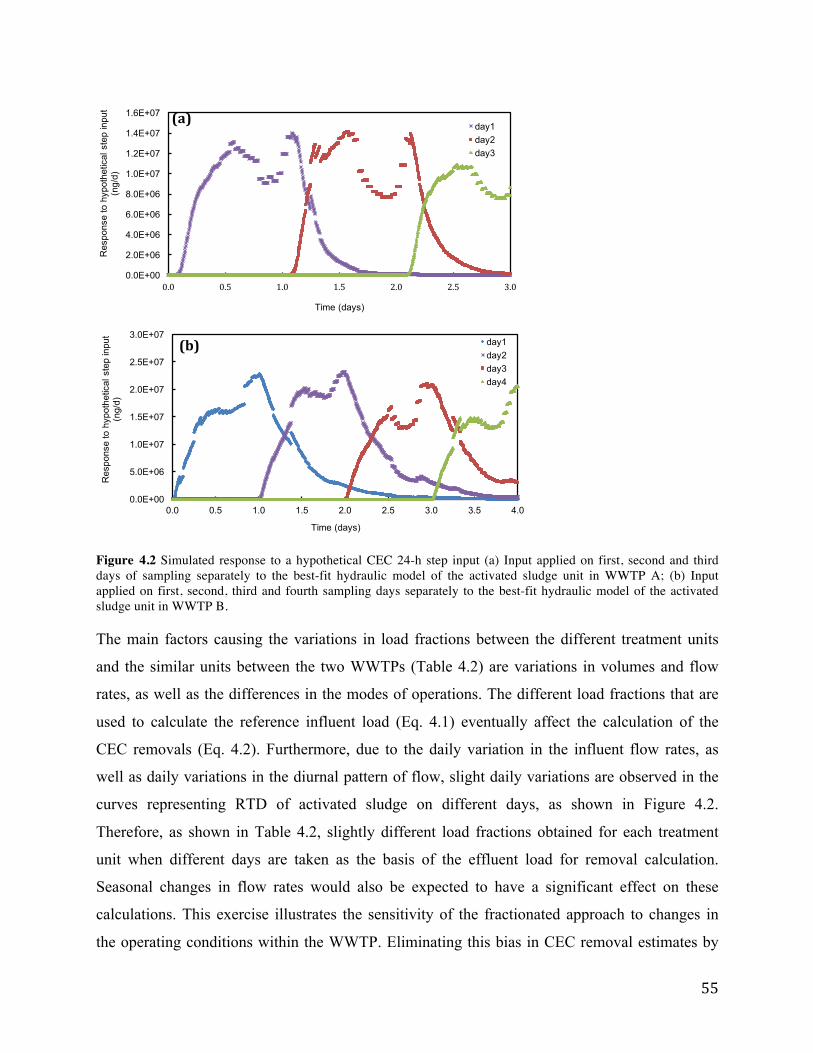
Figure 4.2 Simulated response to a hypothetical CEC 24-h step input (a) Input applied on first, second and third days of sampling separately to the best-fit hydraulic model of the activated sludge unit in WWTP A; (b) Input applied on first, second, third and fourth sampling days separately to the best-fit hydraulic model of the activated sludge unit in WWTP B.

The main factors causing the variations in load fractions between the different treatment units

and the similar units between the two WWTPs (Table 4.2) are variations in volumes and flow

rates, as well as the differences in the modes of operations. The different load fractions that are

used to calculate the reference influent load (Eq. 4.1) eventually affect the calculation of the

CEC removals (Eq. 4.2). Furthermore, due to the daily variation in the influent flow rates, as

well as daily variations in the diurnal pattern of flow, slight daily variations are observed in the

curves representing RTD of activated sludge on different days, as shown in Figure 4.2.

Therefore, as shown in Table 4.2, slightly different load fractions obtained for each treatment

unit when different days are taken as the basis of the effluent load for removal calculation.

Seasonal changes in flow rates would also be expected to have a significant effect on these

calculations. This exercise illustrates the sensitivity of the fractionated approach to changes in

the operating conditions within the WWTP. Eliminating this bias in CEC removal estimates by

accounting for hydraulics is essential, especially when comparing the efficiency of different

treatment stages or trains in removing CECs. The CEC removal efficiencies in primary and

secondary treatment obtained by applying the fractionated approach are discussed in Sections

4.5.3 and 4.5.4.

4.5.2. Concentrations of target contaminants

The average measured concentrations and the calculated mass loads of CECs in the influent and

effluent streams of both WWTPs are summarized in Table 4.3. In the influent streams for both

WWTPs, the average concentrations of the target CECs ranged from 6 ng/L for estrone to 4,400

ng/L for sucralose at WWTP A and from 7 ng/L for estrone to 40,800 ng/L for caffeine at

WWTP B. Trimethoprim was not detected in the influent of both WWTPs, while MDA and

dihydrocodeine were not detected in the influent for WWTP A, but were detected in the influent

at WWTP B. Codeine, morphine and sulfamethoxazole were not detected in the influent of

WWTP B only (Table 4.3). These data illustrate the potential impact of the different populations

on loadings of CECs into domestic wastewater. In general, no significant variations were

observed for any of the CECs in the influent of WWTP A during the sampling period. The ratio

of benzoylecgonine to cocaine concentrations was calculated to be 4.1 in WWTP A and 3.1 in

WWTP B. According to Ratola et al. (2012), the majority of studies report a ratio of 3.1-3.5 in

wastewater. It was suggested that a ratio (benzoylecgonine:cocaine) lower than 5 indicates that

some cocaine was discharged directly into sewage without being consumed and metabolized

(Karolak et al., 2010).

In the effluent of secondary treatment of both WWTPs investigated, some compounds were

<LOD or <LOQ, although they were detected in the influent, including sulfamethoxazole,

cocaine and androstenedione for WWTP A and acetaminophen, ibuprofen, benzoylecgonine,

amphetamine, MDA, dihydrocodeine, estrone and triclosan for WWTP B. The concentrations of

sucralose were the highest of all target CECs in the effluent of both WWTPs, with average

concentrations of around 5600 ng/L and 1100 ng/L in WWTP A and B, respectively.

Table 4.2 Load fractions of influent loads composing the effluent on a given day for the different treatment units in WWTP A and WWTP B. “fi” denotes the fraction of influent load entering on day i that is contained in effluent of day 4, 3 or 2 (second column).

WWTP Based on Load fractions of primary clarifier

Load fractions of aeration tanks Load fractions of secondary clarifier

Load fractions of activated sludge

f1 f2 f3 f4 f1 f2 f3 f4 f1 f2 f3 f4 f1 f2 f3 f4 WWTP A Day 3 effluent 0.0 9.9 90.1 - 0.0 10.5 90.1 - 0.0 12.4 88.2 - 0.3 31.2 69.1 -

Day 2 effluent 10.2 90.1 - - 10.6 89.5 - - 9.7 90.0 - - 32.9 68.5 - - WWTP B Day 4 effluent - - - - 0.0 1.0 28.4 70.7 0.0 0.0 3.1 97.3 0.5 4.8 38.8 55.0

Day 3 effluent - - - - 0.7 25.7 70.5 - 0.0 2.8 96.9 - 3.8 35.5 55.1 -

Mean concentration (ng/L ± STD) and mean mass loads (mg/d ± STD) of target CECs in the influent to the primary treatment and effluent of the secondary treatment at WWTP A and WWTP B. STD is standard deviation based on different days samples and their replicates (n=9 for WWTP A and n=12 for WWTP B).

Concentrations (ng/L ± STD) Mass loads (g/d ± STD) WWTP A WWTP B WWTP A WWTP B Influent Effluent c Influent Effluent Influent Effluent c Influent Effluent Trimethoprim <LOQ b <LOD a <LOD <LOD <LOQ <LOD <LOD <LOD Sulfamethoxazole 16 ± 6 <LOD <LOD <LOD 0.620 ± 0.224 <LOD <LOD <LOD Acetaminophen NA NA 7475 ± 1012 <LOD NA NA 447 ± 61 <LOD Codeine 2518 ± 77 1278 ± 30 <LOD <LOD 98.9 ± 3 50.1 ± 1.2 <LOD <LOD Ibuprofen 2488 ± 100 114 ± 7 249 ± 13 <LOQ 97.6 ± 3.9 4.46 ± 0.27 14.7 ± 0.8 <LOQ Naproxen 2140 ± 91 343 ± 19 237 ± 15 63 ± 3 84.1 ± 3.5 13.6 ± 0.737 14.0 ± 0.9 3.73 ± 0.18 Carbamazepine 90 ± 2 91 ± 5 23 ± 8 26 ± 3 3.53 ± 0.09 3.59 ± 0.20 1.39 ± 0.46 1.54 ± 0.16 Gemfibrozil 19 ± 0.5 22 ± 2 <LOQ 18 ± 3 0.727 ± 0.018 0.859 ± 0.068 <LOQ 1.04 ± 0.19 Benzoylecgonine 1165 ± 35 112 ± 3 554 ± 29 <LOD 45.7 ± 1.3 4.40 ± 0.13 32.2 ± 1.6 <LOD Cocaine 284 ± 16 < LOD 181 ± 24 133 ± 12 8.14 ± 0.75 <LOD 10.8 ± 1.3 7.96 ± 0.69 Amphetamine 178 ± 5 21 ± 0.5 56 ± 8 <LOD 7.03 ± 0.19 0.825 ± 0.019 3.30 ± 0.45 <LOD EEDP 428 ± 29 448 ± 15 155 ± 18 14 ± 4 16.8 ± 1.2 17.6 ± 0.6 9.14 ± 1.01 0.862 ± 0.217 Ephedrine 1672 ± 49 88 ± 5 902 ± 70 106 ± 6 65.6 ± 1.9 3.47 ± 0.20 53.5 ± 3.9 6.23 ± 0.344 MDA <LOD <LOD 41 ± 5 <LOD <LOD <LOD 2.44 ± 0.30 <LOD Dihydrocodeine <LOD <LOD 467 ± 66 <LOD <LOD <LOD 28.4 ± 3.7 <LOD Methadone 170 ± 4 168 ± 6 18 ± 2 11 ± 0.3 6.67 ± 0.17 6.58 ± 0.25 1.09 ± 0.13 0.645 ± 0.016 Morphine 259 ± 18 33 ± 2 <LOD <LOD 10.2 ± 0.7 1.29 ± 0.08 <LOD <LOD Tramadol 189 ± 7 286 ± 16 43 ± 6 77 ± 3 7.45 ± 0.27 11.2 ± 0.6 2.54 ± 0.34 4.53 ± 0.17 Androstenedione 32 ± 1 <LOQ 55 ± 7 15 ± 5 d 1.27 ± 0.05 <LOQ 3.25 ± 0.39 0.297 ± 0.159 Estrone 6 ± 1 5 ± 1 7 ± 2 <LOQ 0.239 ± 0.041 0.196 ± 0.035 0.393 ± 0.121 <LOQ Triclosan 281 ± 8 28 ± 5 27 ± 3 <LOQ 10.9 ± 0.3 1.08 ± 0.20 1.57 ± 0.18 <LOQ Caffeine NA NA 40899 ± 6558 73 ± 21 NA NA 2434 ± 391 4.24 ± 1.25 Sucralose 4362 ± 223 5578 ± 351 3866 ± 305 1097 ± 147 170 ± 9 218 ± 14 228 ± 14.5 65.0 ± 8.83

a,b <LOD and <LOQ: indicates that the compound concentrations were below the limits of detection or quantification, respectively, c refers to the secondary effluent of WWTP A before the UV disinfection, d Androstenedione’s concentration in the effluent was based on a single day, as on the rest of the days, the concentration was <LOQ

4.5.3. Removals of CECs during primary clarification Removals of CECs during primary clarification were only determined for WWTP A, since

WWTP B does not have a primary clarifier unit. The mass loads of the influent to the primary

clarifier of WWTP A were calculated using the fractionated approach and using both day 2 and

day 3 effluent as the basis of calculation. Results for reference (influent) and effluent mass loads

of all CECs are presented in Figure 4.3, and average removal efficiencies in the primary

treatment process are summarized in Table 4.4. The reference mass loads were generally higher

when based on day 2 effluent than when based on day 3 effluent, which can be explained by the

higher concentrations of most CECs observed in the influent of the second day of sampling. On

the other hand, the effluent mass loads observed on the second and the third days of sampling

(day 2 and day 3) were comparable.

Triclosan was estimated to have the highest removal (94%) in the primary clarifier, which is in

agreement with previously reported results (Behera et al., 2011; Blair et al., 2013b; Winkler et

al., 2007). The high removals in the primary clarifier are likely due to the high log Kow of this

compound (i.e. 4.76), which contributes to partitioning to sludge during the primary treatment

step (Rogers, 1996). In addition to adsorption, some biodegradation of CECs is expected to take

place in the primary clarifier, contributing to removal from the aqueous phase (Jones et al., 2005;

Petrie et al., 2014). Androstenedione, carbamazepine, gemfibrozil, ibuprofen, naproxen and

sucralose had poor removals of 10-20% in the primary clarifier. Poor removal of these

compounds during primary clarification was also reported in previous studies (Behera et al.,

2011; Blair et al., 2013b; Ternes & Joss, 2006; Zorita et al., 2009). It is notable that

androstenedione, which is an intermediate in the biosynthesis of testosterone, was poorly

removed by primary clarification. There are only limited data for this compound in the literature

(Esperanza et al., 2007). In the case of ibuprofen and naproxen that have similar pKa (<4) and

log Kow values (3-4), their removals in the primary clarifier were almost equivalent at 13-15%.

Estrone, which is a metabolite of estradiol, showed negative removal in the primary clarifier.

Negative removals of estrone during primary clarification have also been reported by others

(Andersen et al., 2003; Behera et al., 2011; Carballa et al., 2004; Kirk et al., 2002; Ternes et al.,

1999). These observations were attributed to transformation of estradiol to estrone during

primary clarification (Andersen et al., 2003; Carballa et al., 2004; Verlicchi et al., 2012).

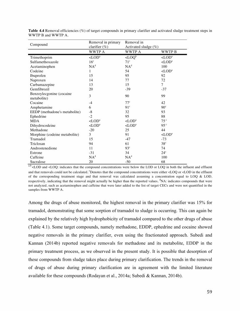
Table 4.4 Removal efficiencies (%) of target compounds in primary clarifier and activated sludge treatment steps in WWTP B and WWTP A.

Compound Removal in primary clarifier (%)

Removal in Activated sludge (%)

WWTP A WWTP A WWTP B Trimethoprim <LODa <LOQb <LODa Sulfamethoxazole 16c 71c <LODa Acetaminophen NAd NAd 100 Codeine 1 54 <LODa Ibuprofen 15 95 92 Naproxen 14 77 72 Carbamazepine 13 15 7 Gemfibrozil 20 -39 -37 Benzoylecgonine (cocaine metabolite) 3 90 99

Cocaine -4 77c 42 Amphetamine 6 91c 90c EEDP (methadone's metabolite) -8 32 93 Ephedrine -2 95 88 MDA <LODa <LODa 75 c Dihydrocodeine <LODa <LODa 95 c Methadone -20 25 44 Morphine (codeine metabolite) 3 91 <LODa Tramadol 15 -47 -73 Triclosan 94 61 38c Androstenedione 11 93c 74 Estrone -31 34 24c Caffeine NAd NAd 100 Sucralose 20 -50 68

a,b <LOD and <LOQ: indicates that the compound concentrations were below the LOD or LOQ in both the influent and effluent and that removals could not be calculated, cDenotes that the compound concentrations were either <LOQ or <LOD in the effluent of the corresponding treatment stage and that removal was calculated assuming a concentration equal to LOQ & LOD, respectively, indicating that the removal might actually be higher than the reported values, dNA: indicates compounds that were not analyzed, such as acetaminophen and caffeine that were later added to the list of target CECs and were not quantified in the samples from WWTP A.

Among the drugs of abuse monitored, the highest removal in the primary clarifier was 15% for

tramadol, demonstrating that some sorption of tramadol to sludge is occurring. This can again be

explained by the relatively high hydrophobicity of tramadol compared to the other drugs of abuse

(Table 4.1). Some target compounds, namely methadone, EDDP, ephedrine and cocaine showed

negative removals in the primary clarifier, even using the fractionated approach. Subedi and

Kannan (2014b) reported negative removals for methadone and its metabolite, EDDP in the

primary treatment process, as we observed in the present study. It is possible that desorption of

these compounds from sludge takes place during primary clarification. The trends in the removal

of drugs of abuse during primary clarification are in agreement with the limited literature

available for these compounds (Rodayan et al., 2014a; Subedi & Kannan, 2014b).

Overall, these results demonstrate that primary clarification has limited capabilities for removing

many of the target CECs, with 14 out of the 17 compounds showing removals < 20% at this step

in the treatment train at WWTP A. This is consistent with these compounds being relatively

hydrophilic and having a low tendency to partition onto solids due to their low log Kow (<3) and

low pKa.

4.5.4. Removal of CECs during activated sludge treatment As with the primary clarifier, the matching mass loads of CECs in the aqueous phase of the

influent and effluent of the activated sludge unit were calculated, as illustrated in Figure 4.4 and

Figure 4.5 for WWTP A and WWTP B, respectively. In WWTP A, the effluent mass loads used

for calculating removals were based on both the second and third sampling days (as for the

primary clarifier), while for WWTP B, it was based on the fourth and third sampling days. The

average removals of target compounds in the activated sludge treatment step for the two WWTPs

are also presented in Table 4.4.

The majority of the removals for most of the target compounds took place in the activated sludge

step, when compared to the low removals in the primary clarifier of WWTP A (Table 4.4).

Amphetamine and benzoylecgonine exhibited removals of >90% during activated sludge

treatment, consistent with previous research on the removal of these two compounds in WWTPs

with activated sludge treatment (Bijlsma et al., 2012; Postigo et al., 2010; Rodayan et al., 2014a).

Acetaminophen and caffeine were shown to undergo substantial removal (WWTP B) of almost

100%, probably due to biodegradation, as suggested in previous studies (Behera et al., 2011;

Kasprzyk-Hordern et al., 2009; Yang et al., 2011). Acetaminophen and caffeine were also shown

to undergo substantial removal (WWTP B) of almost 100%, which is in agreement with previous

studies (Behera et al., 2011; Kasprzyk-Hordern et al., 2009; Yang et al., 2011). Removal

efficiencies of 92-95% and 72-77% were observed for ibuprofen and naproxen, respectively in

the activated sludge process for both WWTPs, which is in good agreement with previous

findings (Behera et al., 2011; Kasprzyk-Hordern et al., 2009; Sim et al., 2010; Yang et al., 2011).

Removals of androstenedione were >93% in WWTP A and 74% in WWTP B. Almost complete

removal of androstenedione from wastewater was previously reported by Esperanza et al. (2007).

Low removals of <40% were observed for estrone and carbamazepine during the activated

sludge treatment at both WWTPs, indicating that these compounds are persistent. These

observations for carbamazepine are consistent with the many studies and databases showing that

carbamazepine is very persistent in WWTPs (Behera et al., 2011; Kasprzyk-Hordern et al., 2009;

Miège et al., 2009; Yang et al., 2011). Estrone was previously reported to be persistent in some

studies (Castiglioni et al., 2006a; Zorita et al., 2009), although other studies reported high

removal (Behera et al., 2011; Miège et al., 2009). The wide range of the CEC removal

efficiencies reported in the literature illustrate the value of the fractionated method for generating

reliable and consistent data on removals of CECs.

Negative removals were observed for tramadol and gemfibrozil in the activated sludge step of

both WWTPs under study, which may be due to the presence of conjugated metabolites in the

influent of the unit that are converted to the parent compound due to the activated sludge

treatment, as was suggested by other authors (Jelic et al., 2011; Lishman et al., 2006). There was

also negative removal of the artificial sweetener, sucralose in the activated sludge unit at WWTP

A, while a positive removal of 68% was calculated for this compound in WWTP B. Among the

limited studies on the fate of sucralose in WWTPs, low removals of sucralose in activated sludge

were previously reported (Pasquini et al., 2013; Subedi & Kannan, 2014a), and a number of

negative removals of sucralose were observed in Norwegian and Swedish WWTPs (Brorström-

Lunden, 2008a; Green, 2007). These were linked to the possibility of the presence of conjugated

and complex forms of sucralose in the influent load, which might transform back to the parent

form during the biological treatment. Negative and variable removals of carbamazepine were

obtained in WWTP A and WWTP B using the day-by-day approach of removal calculation

(results not shown here); however, the fractionated approach yielded positive and consistent

removals.

4.6. Conclusions

In order to obtain reliable data on the removal of CECs during treatment of wastewater, it is

essential to account for mixing regimes that affect the transport of CECs in the WWTP. In this

study, we applied the fractionated approach to characterize CEC removals in two WWTPs.

WWTP B had a longer HRT, as well as a higher degree of mixing deduced from the fractionated

approach than the activated sludge unit in WWTP A, resulting in the need for data over more

sampling days for reliable quantification of removal in WWTP B, as well as different

calculations of CEC removal. The removals of target CECs was generally low or negative in the

primary clarifier and ranged from negative removal to 100% removal over the entire activated

sludge treatment train. This study contributes to advancing the study of the fractionation

approach by applying the approach to treatment steps not investigated before and demonstrating

that the method is able to detect differences in the hydrodynamics of each of the units

investigated at the two treatment plants, resulting in different removal calculations for each unit.

Further, the reliable removals of the extended list of target CECs, obtained in this study by taking

into account hydrodynamics, are key for calibrating fate models of CECs that can be used to

improve our understanding of their fate during treatment and to provide insights for limiting their

discharge.

4.7. Acknowledgements

The authors thank the staff at the two WWTPs for help during the sampling campaigns. We

gratefully acknowledge the McGill Engineering doctoral award for supporting Zeina Baalbaki.

We also thank Brenda McIlwain for preparing samples for analysis at Trent University, and

Craig Murray for his help in deploying temperature/conductivity probes at WWTP A. Funding

for this study was provided by a research grant to Viviane Yargeau (PI) and colleagues from the

Natural Sciences and Engineering Research Council (NSERC) of Canada through the Strategic

Grants Program (430646-2012).

4.8. Supplementary materials:

Table 4.5 Summary of the operating characteristics of the WWTPs and average temperatures during the sampling campaigns.

Characteristic Treatment stage WWTP A WWTP B Hydraulic retention time - HRT (h) Primary clarifier 5.97 -

Aeration tanks 4.52 12.3 Secondary clarifier 3.36 10.6 Total 13.85 22.9

Solid retention time - SRT (days) 10.5 27.6 Average wastewater T (°C) 21 20

Table 4.6 SPE extraction methods and instruments used for compounds of Class a and Class B. Extraction aspect Class A Class B Instrument Gilson GX-271 ASPECTM automated Manual manifold

Cartridge 6 mL-150 mg Oasis MCX cartridges 6 mL-500 mg Oasis MAX cartridges Sample pH pH 2.5 using sulfuric acid pH 8.0 using sodium hydroxide Cartridge 6 mL of acetone and 6 mL of water (pH 2.5) 6 mL of methanol, 6 mL of 0.1 M

Elution 3x3 mL of 5% ammonium hydroxide in 2 mL methanol and then 3x3 mL of 2%

Reconstitution 25% methanol/75% water 50% methanol/50% water

Figure 4.3 Mass loads of target CECs in influent (based on load fractions of two days) and effluent (load on the last day) of the primary clarifier of the WWTP A. Day 1,2,3 represent first, second and third sampling day, respectively. Error bars = one standard deviation of 3 replicates. Sucralose is not shown in this graph, as it has a significantly higher range of mass loads values.

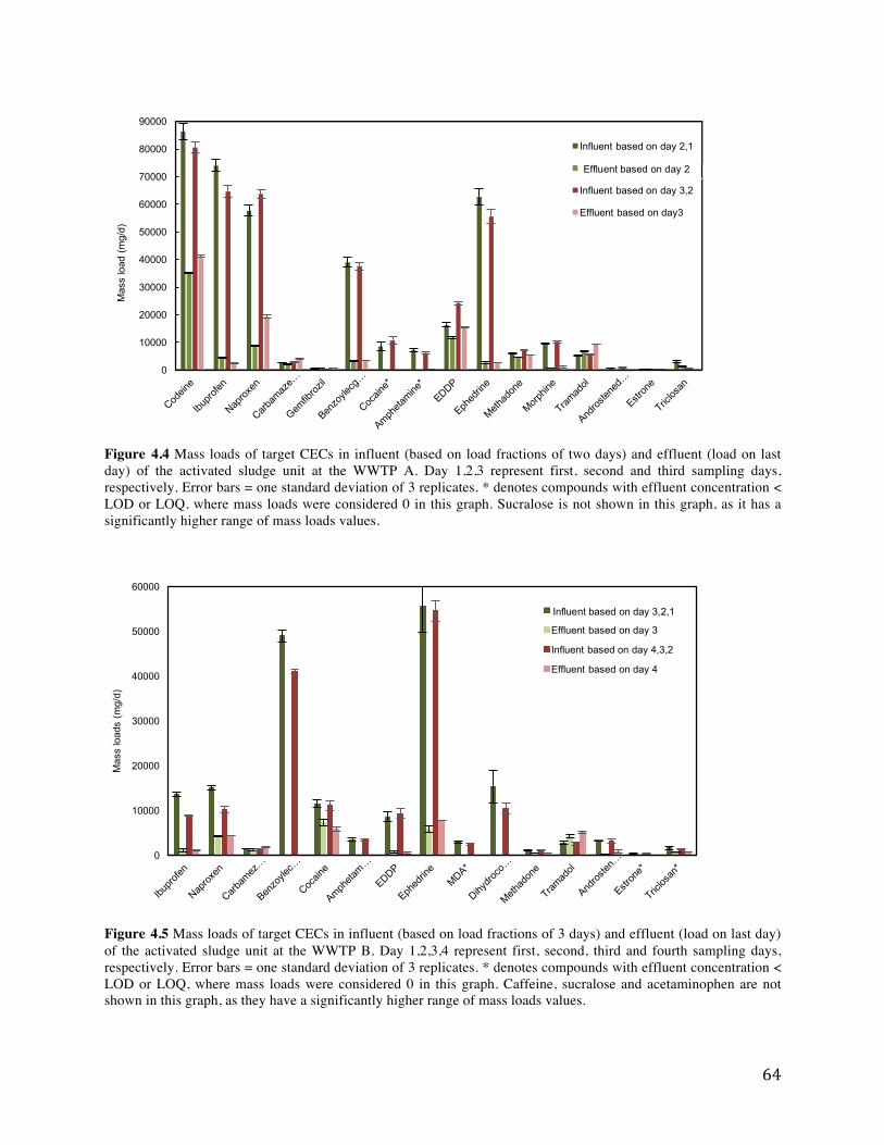
Figure 4.4 Mass loads of target CECs in influent (based on load fractions of two days) and effluent (load on last day) of the activated sludge unit at the WWTP A. Day 1,2,3 represent first, second and third sampling days, respectively. Error bars = one standard deviation of 3 replicates. * denotes compounds with effluent concentration < LOD or LOQ, where mass loads were considered 0 in this graph. Sucralose is not shown in this graph, as it has a significantly higher range of mass loads values.

Figure 4.5 Mass loads of target CECs in influent (based on load fractions of 3 days) and effluent (load on last day) of the activated sludge unit at the WWTP B. Day 1,2,3,4 represent first, second, third and fourth sampling days, respectively. Error bars = one standard deviation of 3 replicates. * denotes compounds with effluent concentration < LOD or LOQ, where mass loads were considered 0 in this graph. Caffeine, sucralose and acetaminophen are not shown in this graph, as they have a significantly higher range of mass loads values.

5. FATE AND MASS BALANCE OF CONTAMINANTS OF EMERGING CONCERN DURING WASTEWATER TREATMENT DETERMINED USING THE FRACTIONATED APPROACH 5.1. Preface

In the previous manuscript (Chapter 4), the CEC removal efficiencies from the aqueous phase in

primary and secondary treatment steps were investigated taking into consideration the effect of

hydrodynamics. In this manuscript, the hydraulics characteristics were also accounted for to

examine the CEC removal in primary and secondary treatment but in a mass balance context to

eventually estimate the CEC load degraded. In addition, the efficiency of tertiary treatment steps

(i.e. rotating biological contactors and sand filters) at removing CECs was assessed for the first

time using the fractionated approach, taking into account the hydraulics of the units. Besides

measuring CECs in the aqueous phase, the portion of CECs sorbed to sludge was quantified in

primary and secondary treatment steps in order to distinguish sorption from other removal

mechanisms. This manuscript addresses two of the objectives of this project: To quantify the

contribution of different fate pathways on the removal of input loads of CECs in primary and

secondary treatment steps and to quantify the removal in tertiary treatment processes while

accounting for the effect of hydraulics.

The WWTP selected for this study uses primary clarification, secondary treatment by activated

sludge and tertiary treatment by both rotating biological contactors and sand filtration. As in the

previous manuscript, an optimum hydraulic model for each treatment unit was identified prior to

sampling. Aqueous samples (24-h composite) were collected in between all the treatment steps,

and grab sludge samples were collected from primary and secondary treatment steps. The target

CECs monitored in this manuscript as well as extraction and chemical analysis procedures were

similar to those in Chapter 4. Mass balance analysis was performed to calculate the difference

between the incoming CEC load and the load sorbed to sludge; which represents the load

transformed by other means, mostly biodegradation.

The optimum hydraulic model structures further demonstrated the unique mixing characteristic

of each treatment unit, resulting in each unit requiring different strategies of calculation of the

CEC removal. Results of the mass balance calculations suggested that each target contaminant

partitioned differently in each fate compartment depending on its physico-chemical properties,

further emphasizing the value of quantifying the contribution of the individual fate pathways.

The majority of the target CECs were observed to have a low tendency to adsorb onto sludge

with the highest affinity to both primary and secondary sludge observed for the antiseptic

triclosan. Removal of CECs by tertiary rotating biological contactors and sand filters, which was

investigated for the first time for some of the target CECs, was generally observed to be low.

This manuscript was accepted for publication in Science of the Total Environment. DOI: http://dx.doi.org/10.1016/j.scitotenv.2016.08.073

Fate and mass balance of contaminants of emerging concern during wastewater treatment determined using the fractionated approach Zeina Baalbaki a, Tamanna Sultana b, Thomas Maere c, Peter A. Vanrolleghem c, Chris D. Metcalfe b, Viviane Yargeau a*

a Department of Chemical Engineering, McGill University, 3610 University St., Montreal, QC, H3A 0C5 b Water Quality Centre, Trent University, 1600 West Bank Drive Peterborough, ON, K9J 7B8 c modelEAU, Département de génie civil et de génie des eaux, Université Laval, 1065 Avenue de la médecine, Québec City, QC, G1V 0A6 * Viviane.yargeau@mcgill.ca

5.2. Abstract

Contaminants of emerging concern (CECs) are often poorly removed from wastewater using

conventional treatment technologies and there is limited understanding of their fate during

treatment. Inappropriate sampling strategies lead to inaccuracies in estimating removals of

CECs. In this study, we used the “fractionated approach” that accounts for the residence time

distribution (RTD) in treatment units to investigate the fate of 26 target CECs in a municipal

wastewater treatment plant (WWTP) that includes primary, secondary and tertiary treatment

steps. Prior hydraulic calibration of each treatment unit was performed. Wastewater and sludge

samples were collected at different locations along the treatment train and the concentrations of

target CECs were measured by liquid chromatography mass spectrometry. The most substantial

aqueous removal occurred during activated sludge treatment (up to 99%). Removals were <50%

in the primary clarifier and tertiary rotating biological contactors (RBCs) and up to 70% by sand

filtration. Mass balance calculations demonstrated that (bio)degradation accounted for up to 50%

of the removal in the primary clarifier and 100% in activated sludge. Removal by sorption to

primary and secondary sludge was minimal for most CECs. Analysis of the selected metabolites

demonstrated that negative removals obtained could be explained by transformations between

the parent compound and their metabolites. This study contributes to the growing literature by

applying the fractionated approach to calculate removal of different types of CECs across each

wastewater treatment step. An additional level of understanding of the fate of CECs was

provided by mass balance calculations in primary and secondary treatments.

Keywords: Adsorption, Fractionated approach, Hydraulics, Micropollutants, Pharmaceuticals

5.3. Introduction:

Contaminants of emerging concern (CECs), including pharmaceuticals and personal care

products (PPCPs), drugs of abuse (DOAs), hormones and stimulants are present in the aquatic

environment (Blair et al., 2013a; Hughes et al., 2013; Rodayan et al., 2015), and these CECs

were found to have adverse effects on aquatic organisms (Gay et al., 2016; Kidd et al., 2007;

Kümmerer, 2008; Purdom et al., 1994). Discharges of wastewater treatment plants (WWTPs)

have been identified as the primary source for CECs introduced into surface waters (Luo et al.,

2014). Therefore, accurate determination of the fate of CECs during wastewater treatment is

required in order to facilitate risk assessments and to identify strategies to improve their removal.

Unexplained temporal variations in the removals of CECs in activated sludge units and in some

cases negative removals (i.e. higher concentration in the effluents than in the influents) have

often been observed in WWTPs, which has raised questions about the appropriateness of the

protocols for sampling wastewater (Majewsky et al., 2011; Ort et al., 2010). In a critical review,

Ort et al. (2010) suggested that sampling strategies that fail to account for the residence time

distribution (RTD), which affects the transport of CECs in treatment units, could result in a

mismatch between the sampled influent and effluent. This mismatch results in biased and

unreliable data on removal efficiencies. Majewsky et al. (2011) proposed a strategy for sampling

and removal calculation referred to as the “fractionated approach” to account for the RTD within

the units of the WWTPs and match the mass loads of the influent with the effluent. This

approach requires prior hydraulic modelling of the WWTP followed by a tailored sampling

strategy where composite samples are collected on several consecutive days. The fractionated

approach has shown promise for evaluating the removal of pharmaceuticals, pesticides and drugs

of abuse during activated sludge treatment (Majewsky et al., 2013; Rodayan et al., 2014a).

However, the fractionated approach has not yet been applied to a complete WWTP treatment

train to identify and quantify the mechanisms of CEC removal at each stage of treatment.

To date, most studies on the removal of CECs did not investigate the contribution of different

removal mechanisms, as they ignored the distribution of CECs between the aqueous and the

particulate compartments (Petrie et al., 2015). A limited number of previous studies have taken a

mass balance approach to determine removals of CECs in conventional primary and secondary

treatment steps through the processes of adsorption and (bio)degradation that were the major

removal mechanisms for the CECs investigated (Carballa et al., 2007; Gao et al., 2012; Heidler

& Halden, 2008; Jelic et al., 2011; Petrie et al., 2014; Wick et al., 2009; Winkler et al., 2007).

The majority of these studies were based on analysis of CECs in grab or 24-h composite

wastewater samples collected simultaneously from different treatment stages, while a small

number of studies accounted for the hydraulic retention time in the sampling campaign but did

not consider the wastewater residence time distribution.

In a recent review, Petrie et al. (2015) identified inadequate sampling approaches, a lack of

understanding of adsorption of CECs onto particulates in WWTPs, as well as a lack of data on

the fate of the metabolites of pharmaceuticals as information gaps that lead to misrepresentative

data of CEC removals. In the present study, advanced sampling strategies that account for the

hydraulic behaviour of treatment units were combined with mass balance analysis to monitor the

fate of 26 target compounds in a WWTP in order to gain insights into the mechanisms of

removal of CECs. The target CECs were contaminants that were reported to be present in surface

water or persistent during wastewater treatment. The list included pharmaceuticals and some of

their metabolites, hormones, drugs of abuse, a stimulant (i.e. caffeine), an artificial sweetener

(i.e. sucralose) and an antibacterial agent (i.e. triclosan). The WWTP monitored in this study

employs primary treatment, secondary treatment by activated sludge, tertiary treatment by both

rotating biological contactors (RBCs) and sand filtration and disinfection by

chlorination/dechlorination. This study contributes to the literature on the use of the fractionated

approach for reliable determination of CEC removals, and for the first time, uses this approach to

estimate removals during the tertiary treatment steps with RBCs and sand filtration. Further, the

predominant removal mechanisms during primary and secondary treatment were identified by

the mass balance analysis.

5.4. Materials and Methods

5.4.1. Chemicals and other supplies The target CECs included several pharmaceuticals identified by Dickenson et al. (2011) in a

study that illustrated the value of monitoring a small number of CECs in WWTPs in the USA.

Sucralose was added to the list as a tracer of wastewater contamination due to its persistence and

ubiquitous presence at high concentrations (Mawhinney et al., 2011). The drugs of abuse were

selected based upon our previous studies indicating their presence in wastewaters in Canada

(Metcalfe et al., 2010; Rodayan et al., 2014a). Androstenedione was selected as a model

androgen because of the lack of data in the literature investigating its fate (Esperanza et al.,

2007), and estrone was selected as a model estrogen because of its widespread occurrence in

wastewater (Servos et al., 2005). To illustrate the importance of including metabolites in mass

balance calculations, two metabolites of carbamazepine, rac trans-10,11-dihydro-10,11-

dihydroxy carbamazepine (CBZ-DiOH) and carbamazepine 10,11-epoxide (CBZ-EP) were

monitored because these compounds have been previously detected in wastewater and sludge

(Hummel et al., 2006; Miao & Metcalfe, 2003; Miao et al., 2005). Other metabolites monitored

in this study included EDDP, the primary metabolite of methadone, and benzoylecgonine, the

primary metabolite of cocaine.

The target CECs, along with their physicochemical properties and the suppliers from which they

were purchased are listed in Table 5.1. The analytes were classified as Class A and B compounds

(Table 5.1) according to the extraction and analysis procedures. Class B compounds are drugs of

abuse and some of their metabolites, which are mainly weak bases, in addition to carbamazepine

and its two metabolites. Class A compounds are all other target compounds that are weak acids,

neutral or phenolic compounds. The internal standards used for each compound are listed in

Table 5.1. 10,11-dihydrocarbamazepine was used as a surrogate for CBZ-DiOH, as performed in

previous studies (Leclercq et al., 2009; Miao & Metcalfe, 2003). All analytical standards and

stock solutions were stored in amber glass vials at -20 °C.

Methanol, acetonitrile, and water of liquid chromatography–mass spectrometry (LC–MS) grade,

as well as other chemicals used for sample preparation were purchased from Fisher Scientific

(Ottawa, ON, Canada). Ultrapure water was generated using a Milli-Q water purification system

(Millipore, Bedford, MA, USA).

Table 5.1: Target CECs and their chemical and physical characteristics, internal standards, class (determining the corresponding extraction and analysis methods), LODs and LOQs in aqueous and biosolids samples and the supplier of the compounds and their surrogates.

Type Subtype Compound Log Kow1 pKa

1 Internal standard (surrogate) Class

Aqueous LOD, LOQ (ng/L) 4

Biosolids LOD, LOQ (ng/L)4

Company5 Compound, surrogate

Pharmaceuticals Antibiotics Trimethoprim 0.91 6.8 Trimethoprim-13C3 A 7,22 3,10 S,I

Sulfamethoxazole 0.89 5.7 Sulfamethoxazole-13C6 A 4,14 2,9 S,I

Analgesics Codeine 1.14 8.2 Codeine-d3 B 6,18 3,9 C,C Ibuprofen 3.97 4.9 Ibuprofen-13C3 A 6,21 10,32 S,I Naproxen 3.18 4.2 Naproxen-13c1-d3 A 4,14 6,19 S,I

Antiepileptic and metabolites

Carbamazepine 2.45 3.2 Carbamazepine-d10 B 2,5 2,6 C,C rac trans-10,11-Dihydro-10,11-dihydroxy Carbamazepine (CMZ-DiOH)

0.13 N.A. 10,11 dihydro carbamazepine B 4,13 3,9 T,T

Carbamazepine 10,11-Epoxide (CMZ-EP) 1.26 N.A. Carbamazepine

10,11-Epoxide-d8 B 2,7 1,5 T,T

Drugs of abuse Cocaine and metabolite

Benzoylecgonine (cocaine’s metabolite) -1.32 N.A. Benzoylecgonine-d3 B 4,14 2,5 C,C

Cocaine 2.3 8.6 Cocaine-d3 B 26,84 11,36 C,C Amphetamines Amphetamine 1.76 10.1 Amphetamine-d5 B 4,13 1,4 C,C

Methamphetamine 2.07 10.2 Methamphetamine-d9 B 7,23 1,4 C,C EDDP (methadone's metabolite) 4.94 9.6 EDDP-d3 B 5,18 4,15 C,C Ephedrine 1.13 9.7 Ephedrine-d3 B 7,25 3,9 C,C

Opioids Dihydrocodeine 1.49 8.8 Dihydrocodeine-d6 B 8,22 5,14 C,C Fentanyl 4.05 8.6 Fentanyl-d5 B 6,20 3,8 C,C Ketamine 2.18 7.5 Ketamine-d4 B 8,27 2,8 C,C Methadone 3.93 8.9 Methadone-d9 B 4,13 1,4 C,C Morphine (codeine metabolite) 0.89 9.9 Morphine-d3 B 5,17 10,32 C,C Oxycodone 0.66 8.3 Oxycodone-d3 B 10,22 3,7 C,C Tramadol 2.63 9.4 Tramadol-d3 B 7,24 1,3 C,C

Personal Care Products Antibacterial Triclosan 4.76 7.9 Triclosan-13C12 A 6,19 6,19 K,M Steroid hormones Androstenedione 2.75 NA Androstene-3,17-

dione-2,3,4-13C3 A 2,5 7,25 S,C

Estrone 3.13 10.3 Estrone-3,4-13C2 A 2,5 6,19 S,I Nervous stimulant Caffeine -0.07 14 Caffeine-13C3 A 4,14 5,16 S,I Artificial sweetener Sucralose -12 11.83 Sucralose-d6 A 7,22 9,30 S,T

1 National Center for Biotechnology Information (2004),2 (Subedi & Kannan, 2014a), 3 (Busetti et al., 2015); 4 LODs and LOQs were obtained based on standard deviation of y-intercept of measured concentrations of serial dilution, 5 Companies: S: Sigma-Aldrich Canada (Oakville, ON, Canada), I: C/D/N Isotopes (Pointe-Claire, QC, Canada), C: Cerilliant Corporation (Round Rock, Tex, USA), M: Cambridge isotope Laboratories (Tewksbury, MA, USA), T: Toronto Research Chemicals (North York, ON, Canada), K: KICTeam (Langely, BC, Canada).

5.4.2. Study site The study site is a municipal WWTP located in Guelph, ON, Canada, serving a population of

approximately 134,894, having a design capacity of 64,000 m3/d and receiving an average

incoming flow rate of 50,755 m3/d of domestic, commercial and industrial wastewater. The

WWTP (Figure 5.1) provides preliminary treatment by screening and aerated grit removal, after

which the load is split into four activated sludge lines. Each of the lines consists of two primary

clarifiers, two aeration tanks and one or two secondary clarifiers in parallel. The WWTP

provides tertiary treatment for the recombined effluent of the lines by rotating biological

contactors (RBCs), followed by sand filtration. The tertiary treatment step was added to the

treatment sequence in order to meet regulations concerning the levels of TSS (i.e. 10 mg/L) and

ammonia nitrogen (i.e. 3.4 mg/L) in the effluent. For disinfection, chlorine is added to

wastewater after the RBCs as 12% sodium hypochlorite at an average chlorine dosage of 1760

kg/d. The disinfected de-chlorinated final effluent is discharged into the Speed River. Table 5.2

summarizes the main characteristics of line 1 in the WWTP since only line 1 was investigated in

in the present study.

Figure 5.1 Schematic of the WWTP. Lines 1-4 correspond to the four lines of primary and secondary treatment. Red marks represent locations where conductivity probes were deployed and aqueous samples were collected. Green marks represent locations where sludge samples were collected.

Aeration basin

Secondary clarifier

Primary clarifier RBC

Sand Filter

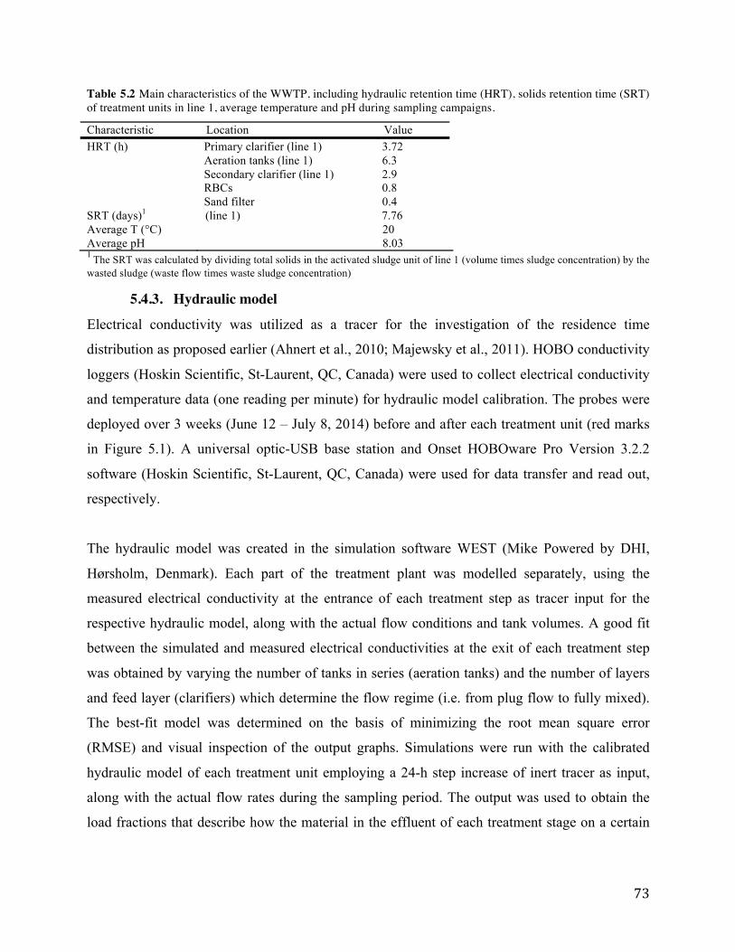
Table 5.2 Main characteristics of the WWTP, including hydraulic retention time (HRT), solids retention time (SRT) of treatment units in line 1, average temperature and pH during sampling campaigns. Characteristic Location Value HRT (h) Primary clarifier (line 1) 3.72

Aeration tanks (line 1) 6.3 Secondary clarifier (line 1) 2.9 RBCs 0.8 Sand filter 0.4

SRT (days)1 (line 1) 7.76 Average T (°C) 20 Average pH 8.03 1 The SRT was calculated by dividing total solids in the activated sludge unit of line 1 (volume times sludge concentration) by the wasted sludge (waste flow times waste sludge concentration)

5.4.3. Hydraulic model Electrical conductivity was utilized as a tracer for the investigation of the residence time

distribution as proposed earlier (Ahnert et al., 2010; Majewsky et al., 2011). HOBO conductivity

loggers (Hoskin Scientific, St-Laurent, QC, Canada) were used to collect electrical conductivity

and temperature data (one reading per minute) for hydraulic model calibration. The probes were

deployed over 3 weeks (June 12 – July 8, 2014) before and after each treatment unit (red marks

in Figure 5.1). A universal optic-USB base station and Onset HOBOware Pro Version 3.2.2

software (Hoskin Scientific, St-Laurent, QC, Canada) were used for data transfer and read out,

respectively.

The hydraulic model was created in the simulation software WEST (Mike Powered by DHI,

Hørsholm, Denmark). Each part of the treatment plant was modelled separately, using the

measured electrical conductivity at the entrance of each treatment step as tracer input for the

respective hydraulic model, along with the actual flow conditions and tank volumes. A good fit

between the simulated and measured electrical conductivities at the exit of each treatment step

was obtained by varying the number of tanks in series (aeration tanks) and the number of layers

and feed layer (clarifiers) which determine the flow regime (i.e. from plug flow to fully mixed).

The best-fit model was determined on the basis of minimizing the root mean square error

(RMSE) and visual inspection of the output graphs. Simulations were run with the calibrated

hydraulic model of each treatment unit employing a 24-h step increase of inert tracer as input,

along with the actual flow rates during the sampling period. The output was used to obtain the

load fractions that describe how the material in the effluent of each treatment stage on a certain

day is composed out of fractions of the influent to that treatment step over several days, as

illustrated by Majewsky et al. (2011).

5.4.4. Wastewater sampling Wastewater was collected before and after each treatment unit at the locations shown in Figure

5.1 (red marks). The number of sampling days was based on the best-fit hydraulic model that

indicated that the effluent of the activated sludge unit on a given day is composed of influent

material entering the WWTP over four days, which will be elaborated upon in the results section.

The samples collected during the first sampling campaign (July 21-25, 2014) were analyzed for

the Class A compounds, while the samples collected during the second campaign (June 16-20,

2015) were analyzed for the Class B compounds. The samples were collected as 24-h composite

using onsite Hach Sigma samplers that collect flow-proportional samples and refrigerate them at

4° C. This is with the exception of the effluent of the RBC, where ISCO 6712 samplers

(Avensys, St-Laurent, QC, Canada) equipped with 24 bottles and packed with ice replaced daily

were used to collect 24-h time-proportional composite samples. Both samplers collected samples

every 15 minutes. Primary and secondary waste sludge samples were collected as grab samples

over the four days (green marks in Figure 5.1). At the end of each day of the sampling campaign,

the collected aqueous and sludge samples were transferred into 1-L amber HDPE bottles (Fisher

Scientific) and stored at -20 °C until extraction was performed (within 3 weeks).

5.4.5. Sample preparation

Wastewater samples were thawed and filtered using 1- m glass-fiber filter (Fisher Scientific)

prior to extraction. Volumes of 100 mL of raw wastewater influent and 200 mL of all other

sample matrixes were spiked with the appropriate internal standards (listed in Table 5.1). Solid

phase extraction (SPE) was performed using two different methods. Class A compounds were

extracted with Oasis MAX anion exchange cartridges (Waters Corporation), as described by

Metcalfe et al. (2014). Class B compounds were extracted with Oasis MCX cation exchange

cartridges, as described by Yargeau et al. (2014a). Both methods and instruments used are

summarized in the supplementary material (Table 5.6). SPE recoveries of target compounds

ranged from 71% to 130% for Class A compounds (average recovery of 75%) and from 60% to

100% for Class B compounds (average recovery of 78%). Glass containers pre-cleaned with

hexanes and acetone were used for all sample preparation and analysis experiments.

Approximately 1 g of freeze-dried sludge was placed in accelerated solvent extraction (ASE)

stainless steel cells and spiked with internal surrogates (Table 5.1, 100 ng/g) before extraction.

Extraction of sludge was conducted by pressurized liquid extraction using a Dionex ASE 350

accelerated solvent extraction system (Thermo Fisher Scientific, Waltham, MA, USA), followed

by SPE clean up based on the methods summarized in the supplementary materials (Table 5.6).

For the Class A compounds, the two extraction methods used were described by Edwards et al.

(2009) as the neutral drug method and the acidic drug method. However, the neutral drugs

method with acetone and water (3:7) as the ASE extraction solvent (Table 5.6) gave the highest

recoveries in the sludge matrix for this study. For class B compounds (mainly drugs of abuse),

the extraction method that achieved the highest recoveries was the one suggested for the beta-

blocker atenolol in the same study by Edwards et al. (2009) and is also summarized in Table 5.6.

All sludge samples were extracted in triplicates and the extraction efficiencies of target

compounds were >70%.

5.4.6. Analysis Analysis of the Class A compounds was performed by liquid chromatography with tandem mass

spectrometry (LC-MS/MS) using an Agilent 1100 HPLC (Mississauga, ON, Canada) coupled to

a Q-Trap 5500 instrument (AB Sciex, Concord, ON, Canada) operated with a turbospray

ionization source. The Class A target compounds of all samples were separated

chromatographically using the method described by Metcalfe et al. (2014). The analytes were

measured in either negative or positive ion mode, depending on the compound. Acquisition was

performed using the precursor and product ion transitions for multiple reaction monitoring

(MRM) of the target compounds and their corresponding deuterated surrogates. The MRM

transitions for the target compounds are listed elsewhere (Metcalfe et al., 2014; Thompson et al.,

2011).

Analysis of the Class B compounds was conducted by liquid chromatography with high-

resolution mass spectrometry (LC-HRMS) using an Accela LC system coupled to a LTQ

Orbitrap XL (Thermo Fisher Scientific, Waltham, MA, USA). Chromatographic separation and

analysis in positive ion mode was achieved using the methods described by Rodayan et al.

(2014b). Acquisition was performed in full scan mode (50–400 m/z) at high resolution (RFWHM

= 41,000). The ion of interest was extracted using an m/z window of ±0.01. Linear calibration

curves of nine points were used for quantification of the concentrations of the target compounds

of both classes. Recoveries of the internal standards were used to adjust the concentrations of all

target analytes.

5.4.7. CEC removals The equations used for the calculations of CEC removals from the aqueous phase are presented

in Eqs. 1-3 and Figure 5.6 in the supplementary material. Calculation of the CEC removals was

first based on the CEC load in the aqueous phase only of the input and output streams of each

treatment unit, as described in Eq. 5.1. To account for the residence time distribution, a

fractionated input load of the CEC that corresponds to the output load on the fourth day of

sampling was calculated (using Eq. 5.2), as proposed by Majewsky et al. (2011). The term “input

reference load” will be used throughout the paper to refer to the incoming fractionated load of

each treatment unit. The input reference load was compared to the output load to obtain estimates

of the CEC removals per treatment unit (Eq. 5.3).

(5.1) (5.2)

(5.3)

Where : Load of the contaminant in the aqueous phase of a specific stream (mg/d), :

Concentration of the contaminant in the aqueous phase of a specific stream (mg/L), : Flow rate

of the corresponding stream (L/d), (mg/d): Input reference mass load of the contaminant

in the aqueous phase of the input stream based on several days of sampling, (mg/d): Mass

load of the contaminant in the input stream on the ith day of sampling, : Fraction of incoming

contaminant load on the ith day of sampling that is contained in the outgoing load on the last day

of sampling, (mg/d): Mass load of the CEC in the aqueous phase of the output stream on

the last day of sampling, (%): Removal of CEC from the aqueous phase in a specific treatment

unit using the fractionated approach.

Mass balances were then carried out across the primary and biological treatment steps based on

the total contaminant load in both aqueous and particulate phases, according to Eq. 5.4-5.7. The

total load of the CEC on each day was obtained in the input stream ( , output stream

( and sludge stream ( by summing particulate and dissolved loads, as shown

in Eq. 5.4. The input reference load was also obtained by the fractionated approach (Eq. 5.6). In

both the primary and biological treatment stages, the primary mechanisms of removal of the

studied CECs are biodegradation and sorption to solids (Andersen et al., 2005; Li & Zhang,

2010; Radjenović et al., 2009b; Verlicchi et al., 2012). Abiotic removal due to hydrolysis or

photolysis was previously investigated for some of the studied CECs and reported to be

negligible (Li & Zhang, 2010; Pèrez et al., 2005). Volatilization is also expected to be limited,

due to the low Henry constants of the studied CECs (Gao et al., 2012). Therefore, the difference

between the total incoming load and the outgoing load (in the output stream or sorbed to sludge)

was assumed to be the load that was lost due to (bio)degradation ( ), as shown in Eq. 5.7. It

should be kept in mind that this load could also include experimental or modelling errors that

could cause a bias in the results.

(5.4)

(5.5)

(5.6)

(5.7)

Where : Mass load of the contaminant in the liquid and particulate phase of a certain stream

(mg/d), : Mass load of contaminant measured in the particulate phase of a stream (mg/d), :

Concentration of contaminant measured in the particulate phase of a stream on a dry weight basis

(mg/g) and : Total suspended solids in the corresponding stream (g/L), which was collected

by the WWTP operators following the APHA/AWWA protocol (Rice et al., 2012). is

computed using Eq. 5.1, except in the sludge stream where the volume fraction of solids is more

significant, so , : Volume fraction of water in sludge,

: Mass load of the contaminant that was (bio)degraded (mg/d).

The measured CEC concentrations were used to calculate the value, defined by Eq. 5.8, to

represent the partitioning of CECs between the dry solids and the aqueous phase for primary and

secondary waste sludge, separately. Error bars for loads, removals and values were obtained

based on standard deviations from lab triplicates using the propagation of error formulas (Ku,

1966). Investigating the statistical significance of the difference between the incoming and the

outcoming loads (Section 5.5.7) was performed using the unequal-variance two-sample t-test

with a confidence level of 95%.

(5.8)

5.5. Results and Discussion

5.5.1. Calibration of hydraulic model and load fractions The hydraulic mixing of the aeration tanks in line 1 was best described by three continuous-

stirred tanks (CSTs) in series, all having equal volume and each representing perfect mixing.

This is consistent with previous studies where the hydrodynamics of the aeration tanks in the

activated sludge process were represented by a number of perfectly mixed tanks in series

(Majewsky et al., 2011; Rodayan et al., 2014a). The primary and secondary clarifiers were both

best modelled with a 10-layer settling tank and the 5th layer as feed layer. Figure 5.7 illustrates

that the simulated and the measured output conductivity profiles were in good agreement for all

treatment steps, verifying the goodness of the fit of the obtained hydraulic model. The RBC

hydraulic behaviour was modelled by a single CST and the sand filter as a series of 2 CSTs. The

volumes for the RBCs and sand filters were adjusted until the simulated effluent matched the

actual hydraulic behaviour, as it was not possible to estimate the actual hydraulic volume. The

obtained volume was small, leading to low retention times, consistent with data obtained from

operators at the WWTP. The absence of significant shifts or damping in the dynamics (Figure

5.7) demonstrates the minimal mixing occurring in both the RBCs and the sand filters due to

their very short HRTs (see Table 5.2).

The obtained load fractions for the removal calculations are summarized in Table 5.3. For a

selected treatment unit, load fractions represent the fractions of CEC incoming load on different

days that make their way to the output on the last day of sampling, assuming no removal. Hence,

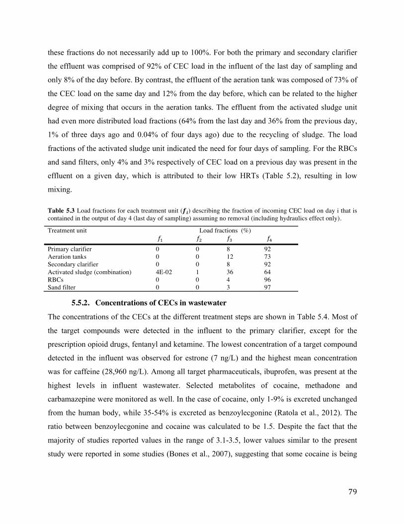
these fractions do not necessarily add up to 100%. For both the primary and secondary clarifier

the effluent was comprised of 92% of CEC load in the influent of the last day of sampling and

only 8% of the day before. By contrast, the effluent of the aeration tank was composed of 73% of

the CEC load on the same day and 12% from the day before, which can be related to the higher

degree of mixing that occurs in the aeration tanks. The effluent from the activated sludge unit

had even more distributed load fractions (64% from the last day and 36% from the previous day,

1% of three days ago and 0.04% of four days ago) due to the recycling of sludge. The load

fractions of the activated sludge unit indicated the need for four days of sampling. For the RBCs

and sand filters, only 4% and 3% respectively of CEC load on a previous day was present in the

effluent on a given day, which is attributed to their low HRTs (Table 5.2), resulting in low

mixing.

Table 5.3 Load fractions for each treatment unit ( ) describing the fraction of incoming CEC load on day i that is contained in the output of day 4 (last day of sampling) assuming no removal (including hydraulics effect only). Treatment unit Load fractions (%)

Primary clarifier 0 0 8 92 Aeration tanks 0 0 12 73 Secondary clarifier 0 0 8 92 Activated sludge (combination) 4E-02 1 36 64 RBCs 0 0 4 96 Sand filter 0 0 3 97

5.5.2. Concentrations of CECs in wastewater The concentrations of the CECs at the different treatment steps are shown in Table 5.4. Most of

the target compounds were detected in the influent to the primary clarifier, except for the

prescription opioid drugs, fentanyl and ketamine. The lowest concentration of a target compound

detected in the influent was observed for estrone (7 ng/L) and the highest mean concentration

was for caffeine (28,960 ng/L). Among all target pharmaceuticals, ibuprofen, was present at the

highest levels in influent wastewater. Selected metabolites of cocaine, methadone and

carbamazepine were monitored as well. In the case of cocaine, only 1-9% is excreted unchanged

from the human body, while 35-54% is excreted as benzoylecgonine (Ratola et al., 2012). The

ratio between benzoylecgonine and cocaine was calculated to be 1.5. Despite the fact that the

majority of studies reported values in the range of 3.1-3.5, lower values similar to the present

study were reported in some studies (Bones et al., 2007), suggesting that some cocaine is being

discharged into the sewage system without consumption (Karolak et al., 2010; Ratola et al.,

2012).

Table 5.4 shows that the CEC concentrations in the combined secondary effluent (i.e. combined

output from all the lines, Figure 5.1) were generally in the same ranges as the concentrations in

the secondary effluent (i.e. from line 1), indicating that in terms of CEC removal, line 1 had a

similar efficiency at removing CECs as the other three lines combined. In the final effluent, some

target compounds, nine out of 26 CECs were not detected at concentrations above the limits of

detection (LODs) or limits of quantification (LOQs). The highest effluent levels were observed

for sucralose (3476 ng/L) followed closely by caffeine (2015 ng/L), unlike in the influent where

caffeine had levels one order of magnitude higher than sucralose.

Table 5.4 Concentrations (ng/L ± standard deviation) of target CECs in line 1 of the WWTP at the influent to the primary clarifier (primary influent), effluent of the primary clarifier (primary effluent), effluent of the secondary clarifier (secondary effluent), as well as the combined secondary effluents of all lines (1-4), and effluent of RBCs (RBCs effluent) and sand filter effluent. Standard deviation was based on 3 replicates of sample preparation and analysis. Compound Primary influent

(Line 1) Primary effluent (Line 1)

Secondary effluent (Line 1)

Combined secondary effluent

RBCs effluent

Sand filter effluent

Androstenedione 92 ± 5 65 ± 2 42 ± 2 41 ± 2 40 ± 1 44 ± 1 Estrone 7 ± 3 8 ± 2 5 ± 1 7 ± 3 5 ± 1 6 ± 2 Trimethoprim 25 ± 2 25 ± 3 37 ± 3 29 ± 3 22 ± 2 <LOD Sulfamethoxazole 33 ± 5 31 ± 5 43 ± 16 47 ± 21 37 ± 6 <LOQ Ibuprofen 3644 ± 105 1690 ± 90 <LOQ <LOQ <LOQ <LOQ Naproxen 471 ± 36 504 ± 35 36 ± 5 20 ± 3 18 ± 2 <LOQ Triclosan 166 ± 26 132 ± 11 50 ± 2 31 ± 4 42 ± 3 29 ± 2 Caffeine 28960 ± 4658 28123 ± 4750 1756 ± 226 2148 ± 127 2245 ± 194 2015 ± 270 Sucralose 2437 ± 220 2635 ± 166 4591 ± 291 3178 ± 84 3175 ± 209 3476 ± 129 Cocaine 361 ± 18 287 ± 30 111 ± 26 97 ± 21 <LOQ <LOQ Benzoylecgonine 524 ± 14 415 ± 18 83 ± 5 58 ± 4 50 ± 2 47 ± 3 Amphetamine 101 ± 2 77 ± 3 <LOQ <LOD <LOD <LOD Methamphetamine 300 ± 7 213 ± 10 47 ± 5 43 ± 2 23 ± 0.2 <LOD EDDP 249 ± 29 299 ± 21 231 ± 55 156 ± 7 169 ± 15 156 ± 4 Ephedrine 1616 ± 62 1053 ± 61 111 ± 8 86 ± 8 72 ± 1 72 ± 3 Codeine 2116 ± 92 1204 ± 40 1281 ± 109 901 ± 16 529 ± 15 130 ± 5 Dihydrocodeine 324 ± 23 459 ± 23 22 ± 1 39 ± 3 28 ± 1 27 ± 1 Methadone 123 ± 3 98 ± 3 48 ± 4 54 ± 2 44 ± 1 42 ± 2 Morphine 295 ± 12 338 ± 61 68 ± 19 24 ± 3 23 ± 4 21 ± 5 Oxycodone 126 ± 10 137 ± 24 64 ± 3 46 ± 3 35 ± 3 27 ± 7 Tramadol 174 ± 6 116 ± 8 177 ± 11 105 ± 5 125 ± 7 105 ± 5 Ketamine <LOD <LOD <LOQ <LOQ <LOQ <LOQ Fentanyl <LOD <LOD <LOD <LOD <LOD <LOD Carbamazepine 591 ± 24 416 ± 20 606 ± 28 588 ± 17 532 ± 8 519 ± 13 CMZ-DIOH 1074 ± 54 702 ± 40 553 ± 51 650 ± 26 703 ± 21 648 ± 49 CMZ-EP 192 ± 36 258 ± 40 295 ± 41 315 ± 44 385 ± 62 119 ± 32

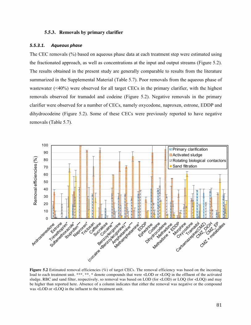
5.5.3. Removals by primary clarifier

The CEC removals (%) based on aqueous phase data at each treatment step were estimated using

the fractionated approach, as well as concentrations at the input and output streams (Figure 5.2).

The results obtained in the present study are generally comparable to results from the literature

summarized in the Supplemental Material (Table 5.7). Poor removals from the aqueous phase of

wastewater (<40%) were observed for all target CECs in the primary clarifier, with the highest

removals observed for tramadol and codeine (Figure 5.2). Negative removals in the primary

clarifier were observed for a number of CECs, namely oxycodone, naproxen, estrone, EDDP and

dihydrocodeine (Figure 5.2). Some of these CECs were previously reported to have negative

removals (Table 5.7).

Figure 5.2 Estimated removal efficiencies (%) of target CECs. The removal efficiency was based on the incoming load to each treatment unit. ***, **, * denote compounds that were <LOD or <LOQ in the effluent of the activated sludge, RBC and sand filter, respectively, so removal was based on LOD (for <LOD) or LOQ (for <LOQ) and may be higher than reported here. Absence of a column indicates that either the removal was negative or the compound was <LOD or <LOQ in the influent to the treatment unit.

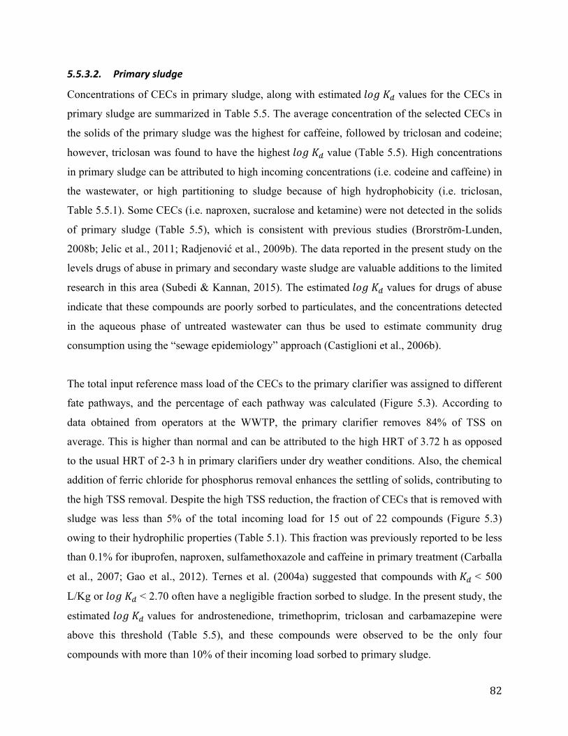
Concentrations of CECs in primary sludge, along with estimated values for the CECs in

primary sludge are summarized in Table 5.5. The average concentration of the selected CECs in

the solids of the primary sludge was the highest for caffeine, followed by triclosan and codeine;

however, triclosan was found to have the highest value (Table 5.5). High concentrations

in primary sludge can be attributed to high incoming concentrations (i.e. codeine and caffeine) in

the wastewater, or high partitioning to sludge because of high hydrophobicity (i.e. triclosan,

Table 5.5.1). Some CECs (i.e. naproxen, sucralose and ketamine) were not detected in the solids

of primary sludge (Table 5.5), which is consistent with previous studies (Brorström-Lunden,

2008b; Jelic et al., 2011; Radjenović et al., 2009b). The data reported in the present study on the

levels drugs of abuse in primary and secondary waste sludge are valuable additions to the limited

research in this area (Subedi & Kannan, 2015). The estimated values for drugs of abuse

indicate that these compounds are poorly sorbed to particulates, and the concentrations detected

in the aqueous phase of untreated wastewater can thus be used to estimate community drug

consumption using the “sewage epidemiology” approach (Castiglioni et al., 2006b).

The total input reference mass load of the CECs to the primary clarifier was assigned to different

fate pathways, and the percentage of each pathway was calculated (Figure 5.3). According to

data obtained from operators at the WWTP, the primary clarifier removes 84% of TSS on

average. This is higher than normal and can be attributed to the high HRT of 3.72 h as opposed

to the usual HRT of 2-3 h in primary clarifiers under dry weather conditions. Also, the chemical

addition of ferric chloride for phosphorus removal enhances the settling of solids, contributing to

the high TSS removal. Despite the high TSS reduction, the fraction of CECs that is removed with

sludge was less than 5% of the total incoming load for 15 out of 22 compounds (Figure 5.3)

owing to their hydrophilic properties (Table 5.1). This fraction was previously reported to be less

than 0.1% for ibuprofen, naproxen, sulfamethoxazole and caffeine in primary treatment (Carballa

et al., 2007; Gao et al., 2012). Ternes et al. (2004a) suggested that compounds with < 500

L/Kg or < 2.70 often have a negligible fraction sorbed to sludge. In the present study, the

estimated values for androstenedione, trimethoprim, triclosan and carbamazepine were

above this threshold (Table 5.5), and these compounds were observed to be the only four

compounds with more than 10% of their incoming load sorbed to primary sludge.

Table 5.5 Average concentrations of target CECs in primary and activated sludge and the range of concentrations on the four days of sampling represented as average (lowest –highest), along with the estimated ± standard deviation in primary and activated sludge.

Compound Average Concentrations (Lowest-highest) (ng/L)

± standard deviation (Log L/Kg)

Primary sludge Activated sludge Primary clarifier Secondary clarifier Androstenedione 98 (85-113) 39 (15-65) 3.20 ± 0.19 2.92 ± 0.37 Estrone <LOD 28 (<LOD-53) <LOD 3.65 ± 0.32 Trimethoprim 31 (24-43) 154 (92-198) 3.07 ± 0.19 3.59 ± 0.18 Sulfamethoxazole 12 (6-17) <LOQ 2.15 ± 0.49 <LOQ Ibuprofen1 196 (73-496) 39 (21-59) 2.27 ± 0.64 3.36 ± 0.38 Naproxen <LOD 23 (<LOQ-25) <LOD 2.95 ± 0.32 Triclosan 599 (340-909) 1335 (1199-1377) 3.68 ± 0.11 4.49 ± 0.27 Caffeine 2828 (1536-4716) 776 (674-953) 2.10 ± 0.37 2.73 ± 0.31 Sucralose <LOD 152 (110-218) <LOD 1.53 ± 0.19 Cocaine 27 (16-35) <LOD 1.93 ± 0.18 <LOD Benzoylecgonine 5 (<LOD-8) <LOQ 1.40 ± 0.07 <LOQ Amphetamine1 20 (7-37) 13 (5-20) 2.29 ± 0.38 3.09 ± 0.33 Methamphetamine 14 (11-17) 4 (<LOD-4) 1.83 ± 0.02 1.92 EDDP 89 (73-109) 65 (44-95) 2.46 ± 0.1 2.44 ± 0.17 Ephedrine 47 (22-69) 26 (<LOQ-55) 1.60 ± 0.48 2.16 ± 0.5 Codeine 202 (77-305) 36 (<LOQ-53) 2.17 ± 0.26 1.36 ± 0.4 Dihydrocodeine 29 (10-44) 41 (18-56) 1.71 ± 0.08 3.20 ± 0.31 Methadone 49 (7-125) 46 (<LOQ-125) 2.57 2.55 ± 0.71 Morphine 96 (40-171) 76 (37-117) 2.61 ± 0.4 2.99 ± 0.29 Oxycodone 25 (9-42) 8 (<LOD-13) 2.09 ± 0.45 1.97 ± 0.44 Tramadol 92 (21-232) 7 (<LOD-11) 2.58 ± 0.5 1.49 ± 0.36 Ketamine <LOQ <LOQ <LOQ <LOQ Fentanyl 18 (11-27) 23 (15-31) N.A. N.A. Carbamazepine2 49 (32-78) 27 (22-34) 2.75 ± 0.21 2.29 ± 0.04 CMZ-DiOH <LOD <LOD <LOD <LOD CMZ-EP <LOD <LOD <LOD <LOD 1Denotes compounds that were <LOD or LOQ in the secondary effluent, indicating that the obtained in the secondary clarifier might not be accurate as it was based on the LOD or LOQ of the compound, 2Carbamazepine solids analysis was based on the 2014 sampling campaign.

Despite the generally low biological activity of primary clarifiers, some of the removal during

primary clarification can be attributed to (bio)degradation, as shown in Figure 5.3. The

percentage of incoming load degraded during primary clarification was as high as 40-54% for a

number of the investigated CECs (i.e. ibuprofen, morphine, codeine, triclosan and ephedrine).

Considering the small error bars of the mass loads in Figure 5.3 (except for triclosan), this high

(bio)degradation in the primary clarifier is unlikely attributed to measurement bias caused by

sample preparation and analysis. McCall et al. (2016) showed in a review article that several

studies reported the formation of transformation products of drugs of abuse in the sewers (HRT

30 min to 12 h) under different conditions, and Heuett et al. (2015) reported the detection of

transformation products of drugs of abuse in influent sewage to a WWTP. The degradation of

some pharmaceuticals and formation of transformation products in a real sewer pipe was also

reported by Jelic et al. (2015). Having similar conditions as in sewers, primary clarifiers could

also allow (bio)degradation of CECs. In addition, the primary clarifier under study has a higher

HRT (3.72 h) than usual, which could explain the high observed CEC (bio)degradation. In fact,

most of the compounds with the highest (bio)degradation in the primary clarifier also showed

high (bio)degradation potential in the activated sludge (Figure 5.4). It should be noted that the

sum of the percentages removed by (bio)degradation and removed with sludge (Figure 5.3) is not

equivalent to the percentage removal from the aqueous phase calculated previously (Figure 5.2).

This is explained by the fact that the input reference mass load used in the mass balance

calculations includes not only CEC loads in the aqueous phase, but also in the particulate phase.

The CEC concentrations in the suspended particulate phase of primary inlet load were assumed

to be equal to those in primary sludge, making the assumption that equilibrium partitioning of

CECs between the particulate and aqueous phases takes place before the primary clarifier.

Figure 5.3 Input reference mass loads (g/d) of target CECs into the primary clarifier assigned into three main fate pathways: (bio)degraded, discharged with primary sludge and discharged with the primary effluent with the % contribution of each pathway indicated in the corresponding column (COC: cocaine, BG: benzoylecgonine, MTD: methadone). For caffeine (not shown due to the high mass loads): 14% biodegraded, 2% sorbed to primary sludge and 84% in the effluent.

5.5.4. Removals by activated sludge

The estimated removals of CECs (%) during the activated sludge treatment step are illustrated in

Figure 5.2. In general, for the majority of the compounds, most of the removal takes place in the

activated sludge treatment stage when compared to other treatment steps. Amongst the target

compounds, the removals varied from >80% for six target CECs, namely ibuprofen, naproxen,

amphetamine, ephedrine, dihydrocodeine and caffeine to negative removals for carbamazepine,

tramadol, estrone, sucralose and trimethoprim. The variable data on CEC removal by activated

sludge treatment reported in the literature is summarized in the supplementary material (Table

5.7).

The measured concentrations of CECs in the solids of secondary sludge and estimates of the

values for secondary sludge are summarized in Table 5.5. Triclosan followed by caffeine

and trimethoprim were shown to have the highest average concentrations in secondary sludge.

Similar to the analysis of the primary sludge, triclosan had the highest estimated value

(i.e. 4.49) for secondary sludge. Caffeine and sucralose ( -0.07 and -1, respectively), on

the other hand, had high concentrations in secondary waste sludge (Table 5.5) owing to their

high loads to the biological treatment (Table 5.4). The differences in the estimated values

between primary and secondary waste sludge for each of the CECs can be explained by variable

sludge composition (Ternes et al., 2004a).

Figure 5.4 displays the CEC input reference load to the activated sludge unit assigned to different

fate pathways. The reference mass loads were calculated based on the assumption that the CEC

concentrations in the suspended solids contained in the output of the primary and secondary

clarifiers were the same as those measured in the primary and secondary sludge, respectively.

This involves making the assumption that the CEC particulate concentration is uniform

throughout the primary and secondary clarifiers. Discharge with the secondary waste sludge was

found to be the predominant removal mechanism for trimethoprim, triclosan and estrone, with

55%, 51% and 33% of their input reference load, respectively ending up in the secondary waste

sludge. For all the remaining compounds, a low fraction (i.e. <5%) of the input reference load

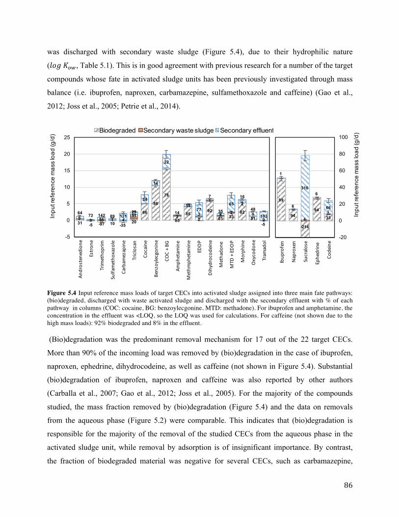
was discharged with secondary waste sludge (Figure 5.4), due to their hydrophilic nature

( , Table 5.1). This is in good agreement with previous research for a number of the target

compounds whose fate in activated sludge units has been previously investigated through mass

balance (i.e. ibuprofen, naproxen, carbamazepine, sulfamethoxazole and caffeine) (Gao et al.,

2012; Joss et al., 2005; Petrie et al., 2014).

Figure 5.4 Input reference mass loads of target CECs into activated sludge assigned into three main fate pathways: (bio)degraded, discharged with waste activated sludge and discharged with the secondary effluent with % of each pathway in columns (COC: cocaine, BG: benzoylecgonine, MTD: methadone). For ibuprofen and amphetamine, the concentration in the effluent was <LOQ, so the LOQ was used for calculations. For caffeine (not shown due to the high mass loads): 92% biodegraded and 8% in the effluent.

(Bio)degradation was the predominant removal mechanism for 17 out of the 22 target CECs.

More than 90% of the incoming load was removed by (bio)degradation in the case of ibuprofen,

naproxen, ephedrine, dihydrocodeine, as well as caffeine (not shown in Figure 5.4). Substantial

(bio)degradation of ibuprofen, naproxen and caffeine was also reported by other authors

(Carballa et al., 2007; Gao et al., 2012; Joss et al., 2005). For the majority of the compounds

studied, the mass fraction removed by (bio)degradation (Figure 5.4) and the data on removals

from the aqueous phase (Figure 5.2) were comparable. This indicates that (bio)degradation is

responsible for the majority of the removal of the studied CECs from the aqueous phase in the

activated sludge unit, while removal by adsorption is of insignificant importance. By contrast,

the fraction of biodegraded material was negative for several CECs, such as carbamazepine,

sucralose, trimethoprim and tramadol, which indicated that the mass loads in the secondary

output were higher than the incoming loads, consistent with their negative removal from the

aqueous phase (Figure 5.2). The use of the fractionated approach accounting for RTD of the

treatment units limited the bias associated with the sampling strategy and removal calculations

but some negative removals were still observed. These negative removals are, therefore, likely

due to the presence of conjugated forms of the compound that transform into the parent

compound during treatment, as well as desorption from particulate matter (Jelic et al., 2011;

Ternes & Joss, 2006). For carbamazepine and trimethoprim, the absence of removal by

biodegradation obtained in this study is in agreement with previous studies (Gao et al., 2012;

Joss et al., 2005; Li & Zhang, 2010; Petrie et al., 2014).

5.5.5. Removals by RBCs The WWTP was upgraded to include RBCs in order to meet regulations with regards to the

ammonia nitrogen levels in the effluent (i.e. maximum concentration of 3.4 mg/L). Although the

ammonia nitrogen in the secondary effluent was reported to be <1 mg/L during the summer,

indicating full nitrification by the activated sludge process, levels as high as 6.6 mg/L were

observed over several days during the winter. The RBCs removed ammonia nitrogen and

achieved effluent levels below 2.41 mg/L throughout the year. In spite of their capability to

remove ammonia nitrogen, the RBCs were generally ineffective at removing most of the target

CECs (i.e. <30%), except for methamphetamine, codeine and dihydrocodeine, as shown in

Figure 5.2. Additionally, the CECs whose removal calculation had to be based on LOQ or LOD

due to the fact that they were below these limits (marked with two stars) could also have high

removals. Among the target CECs, low average removals of <15% were observed for 11 of the

26 target CECs. Negative removals at this treatment stage were observed for sucralose and

triclosan, indicating the possible de-conjugation of their conjugates during tertiary treatment, as

in the activated sludge treatment stage or possible sampling bias. The fate of a limited number of

the target compounds (i.e. trimethoprim, sulfamethoxazole, triclosan, ibuprofen, carbamazepine

and caffeine) has been investigated before in RBCs, and their obtained removals were higher

than in the present study (Batt et al., 2007; Kanda et al., 2003; Thompson et al., 2005; Vasiliadou

et al., 2014). This can be explained by the fact that the RBCs are used as tertiary treatment in this

study, with a low HRT (i.e. 0.8 h) and little organic material available for biofilm growth, while

in the previous studies, RBCs were used for secondary treatment as an alternative to activated

sludge treatment. The contribution of the particulate CEC load to the total load in the RBCs and

the sand filter is deemed insignificant, since the TSS load entering these units is low (<20 mg/L).

Hence, a detailed mass balance was not performed for these units.

5.5.6. Removals by sand filtration Similar to the RBCs, the average removal of CECs by sand filtration and chlorination was based

on the incoming load in the aqueous phase only, due to the low TSS load. The removal was

greater than 50% for only 4 CECs (i.e. trimethoprim, sulfamethoxazole, morphine and CBZ-EP).

The incoming loads of trimethoprim and sulfamethoxazole were reduced by more than 69% and

58%, respectively by sand filtration. Data from previous studies reported considerable removal

(over 60%) of trimethoprim in sand filters (Göbel et al., 2007; Nakada et al., 2007; Sui et al.,

2010), but lower removals (i.e. 20-30%) were reported for sulfamethoxazole (Gao et al., 2012;

Göbel et al., 2007; Nakada et al., 2007). With the exception of the four compounds listed above,

sand filtration and chlorination were inefficient at removing most of the other target CECs, as

less than 30% of their incoming load was removed (Figure 5.2). The observed removal for

triclosan was similar to that observed by Nakada et al. (2007) (i.e. 29%). Negative removals (or

no removal) were obtained for estrone, sucralose, carbamazepine and CBZ-DiOH during the

sand filtration and chlorination steps. For estrone and carbamazepine, the negative removals are

in agreement with previous studies (Gao et al., 2012; Nakada et al., 2007; Sui et al., 2010),

indicating possible desorption of these compounds during sand filtration. Removal from the

aqueous phase in sand filters is attributed to adsorption to solid particles that are retained by the

sand filter. However, previous studies also indicated that (bio)degradation may contribute to

CEC removal due to the formation of biofilm on sand particles (Göbel et al., 2007). In the

WWTP investigated, chlorine was added right before sand filtration, which makes the growth of

a biofilm unlikely.

5.5.7. Metabolites The combined loads of parent compounds and their metabolite(s) were considered for some

target CECs when calculating removal efficiencies for each treatment stage (Figure 5.5) to

account for possible inter-transformations. Cocaine and its major metabolite had comparable

removals in all treatment units. Although EDDP (methadone’s major metabolite) alone exhibited

negative removal of -17% in the primary clarifier, the removal efficiency based on combined

concentrations of EDDP and its parent compound methadone was above zero, indicating that

some of the methadone was possibly converted into EDDP. Similarly, removals based on

combined loads were obtained for carbamazepine and its two investigated metabolites, CBZ-

DiOH and CBZ-EP. A limited number of studies have investigated the removals of

carbamazepine and its major metabolites in WWTPs (Hummel et al., 2006; Leclercq et al., 2009;

Miao et al., 2005). Only the study by Miao et al. (2005) examined the concentrations of

carbamazepine and its metabolites at each treatment step of the WWTP and observed a decline in

the concentration of carbamazepine and its two metabolites in the primary clarifier and an

increase in carbamazepine and CBZ-DiOH concentrations by activated sludge. In the present

study, the calculation was further refined by considering the input and output mass loadings of

carbamazepine and its two major metabolites in each treatment unit taking the RTD into account,

as shown in Figure 5.5. It should be noted that in the present study, due to use of the fractionated

approach, the input reference load a treatment step is not equivalent to the output load of the

previous treatment step (Figure 5.5).

A decrease was observed in the loads of carbamazepine and CBZ-DiOH during primary

clarification (p<0.05), whilst the variations in the loads of CBZ-EP across the primary clarifier

were not statistically different (p=0.26). Similarly, activated sludge was not shown to cause a

decrease in the loads of carbamazepine and CBZ-EP (p=0.57 and 0.07, respectively), but it

decreased the loads of CBZ-DIOH (p<0.05) and, thus, the combined load of carbamazepine and

its metabolites. This is possibly explained by partial transformation of CBZ-DiOH back into

carbamazepine during both primary clarification and activated sludge causing the persistence of

carbamazepine by compensating for the (bio)degraded load. Tertiary treatment in the form of

RBCs diminished the load of carbamazepine and CBZ-DiOH significantly (p<0.05), but not that

of CBZ-EP (p=0.25). Sand filtration and chlorination, on the other hand, resulted in a decrease in

the average load of only CBZ-EP, accompanied with a load increase of both carbamazepine and

CBZ-DiOH (p<0.05 for all the compounds). The combined load of carbamazepine and the two

metabolites was also increased (p=0.03). This might suggest the transformation of CBZ-EP to

both CBZ-DiOH and carbamazepine during the sand filtration step. The two metabolites of

carbamazepine were not quantified in sludge samples in the present study. However, Miao et al.

(2005) concluded that these compounds are present at low concentrations in biosolids (<8 ng/g).

Figure 5.5 Mass loads of carbamazepine and its two investigated metabolites (CMZ-DiOH & CMZ-EP) in both the input (reference load) and the output of the primary clarifier, secondary treatment, RBCs and sand filter. The numeric values of the load are presented in the columns.

5.6. Conclusions

Removal data for the aqueous phase showed that most CECs were poorly removed (i.e. <40%) in

the primary clarifier. The greatest removals typically occurred in the activated sludge, while

removals were <50% in the RBCs and ranged from no removal to 70% removal during sand

filtration. The mass balances, which looked at dissolved as well as adsorbed CECs provided

further insight into the predominant removal mechanisms for CECs during primary and

secondary treatment. It showed that not only sorption to the primary sludge, but also

(bio)degradation contribute to the removal of some of the target CECs in the primary clarifier. In

activated sludge, (bio)degradation was found to be the predominant removal mechanism, with

sorption accounting for <5% for most CECs. The estimated values (1.40 to 3.68 in

primary sludge and 1.36 to 4.49 in activated sludge) also indicated that most CECs are not

significantly removed by partitioning onto sludge, with the exception of triclosan. Accounting

for the levels of metabolites of the selected CECs (i.e. carbamazepine, methadone and cocaine)

explained some of the negative removals that were observed. The current study expands the

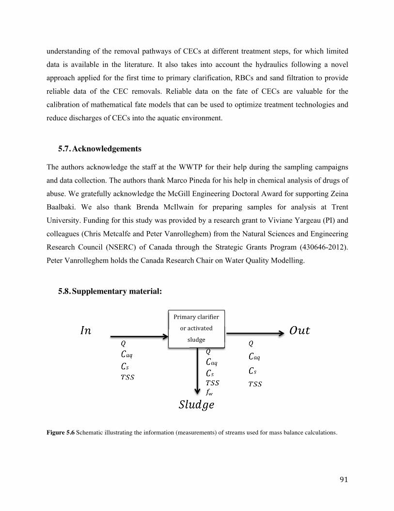
understanding of the removal pathways of CECs at different treatment steps, for which limited

data is available in the literature. It also takes into account the hydraulics following a novel

approach applied for the first time to primary clarification, RBCs and sand filtration to provide

reliable data of the CEC removals. Reliable data on the fate of CECs are valuable for the

calibration of mathematical fate models that can be used to optimize treatment technologies and

reduce discharges of CECs into the aquatic environment.

5.7. Acknowledgements

The authors acknowledge the staff at the WWTP for their help during the sampling campaigns

and data collection. The authors thank Marco Pineda for his help in chemical analysis of drugs of

abuse. We gratefully acknowledge the McGill Engineering Doctoral Award for supporting Zeina

Baalbaki. We also thank Brenda McIlwain for preparing samples for analysis at Trent

University. Funding for this study was provided by a research grant to Viviane Yargeau (PI) and

colleagues (Chris Metcalfe and Peter Vanrolleghem) from the Natural Sciences and Engineering

Research Council (NSERC) of Canada through the Strategic Grants Program (430646-2012).

Peter Vanrolleghem holds the Canada Research Chair on Water Quality Modelling.

5.8. Supplementary material:

Figure 5.6 Schematic illustrating the information (measurements) of streams used for mass balance calculations.

Figure 5.7 Effluent tracer (electrical conductivity ( S/cm)) trends measured (blue) and predicted by the best-fitting hydraulic model (dashed red) throughout four consecutive days for: a) primary clarifier, b) aeration tanks, c) RBCs and d) sand filter.

Table 5.6 Extraction methods of wastewater and biosolids samples for Class A and Class B compounds using solid phase extraction (SPE) for aqueous samples and accelerated solvent extraction couple to SPE (ASE-SPE) for biosolids.

Sample type Method Extraction step Class A Class B Aqueous

SPE Instrument Manual manifold Gilson GX-271 ASPECTM automated instrument

Cartridge 6 mL-500 mg Oasis MAX cartridges

6 mL-150 mg Oasis MCX cartridges

Sample pH pH 8.0 using sodium hydroxide pH 2.5 using sulfuric acid Conditioning Methanol, 0.1 M ammonium

hydroxide and Milli-Q water (pH 8.0)

Acetone and Milli-Q water (pH 2.5)

Elution 2 mL methanol and then 3x3 mL of 2% formic acid in methanol, 1 mL/min

3x3 mL of 5% ammonium hydroxide in methanol, 1 mL/min

Reconstitution 50% methanol/50% water to a total volume of 0.4 mL

25% methanol/75% water to a total volume of 0.4 mL

Biosolids

ASE Instrument Dionex ASE 350 Dionex ASE 350 Conditions Temperature =80 °C

Static cycle= 3 Temperature =50 °C Static cycles= 2

Elution solvent Acetone: water (3:7) Methanol:water:acetic acid (49:49:2)

SPE Instrument Manual manifold Gilson GX-271 ASPECTM automated instrument

Cartridge 6 mL-500 mg Oasis HLB cartridges

6 mL-150 mg Oasis MCX cartridges

Sample pH pH 7.5 using sodium hydroxide pH 2.5 using sulfuric acid Conditioning Acetone, Methanol and Milli-Q

water (pH 7.5). Acetone and Milli-Q water (pH 2.5)

Elution 3x3 mL of methanol, 1 mL/min 3x3 mL of 5% ammonium hydroxide in methanol, 1 mL/min

Reconstitution 50% methanol/50% water to a total volume of 0.1 mL

25% methanol/75% water to a total volume of 0.4 mL

Table 5.7 Average estimated removal efficiencies of target CECs in activated sludge and primary clarifier, separately from previous studies that investigated the removal from the aqueous phase (Please refer to Table 2.4 in the literature review).

6. DYNAMIC MODELLING OF SOLIDS IN FULL-SCALE ACTIVATED SLUDGE PLANT PRECEDED BY CEPT AS A BASIC STEP FOR MICROPOLLUTANT REMOVAL MODELLING 6.1. Preface

The fate of conventional pollutants, such as solids and biomass, as well as the concentration of

dissolved oxygen in the activated sludge process significantly influence the extent at which

CECs are biodegraded or adsorbed to sludge. Hence, for unbiased prediction of the fate of CECs

in activated sludge treatment, which is the last objective of this PhD project, the fate of

conventional pollutants must first be accurately predicted. This is addressed in details in the

current manuscript.

The full-scale activated sludge unit used for calibration in this manuscript is part of the same

WWTP examined in Chapter 7 for the prediction of the fate of CECs. Measurements of

conventional pollutants and dissolved oxygen at different locations of the activated sludge unit

under study were obtained from the operators over one year. In addition, extra measurements

necessary for the characterization of the influent (i.e. the representation of the input in terms of

model components) were collected over three days. An Activated Sludge Model that has an

extension for the prediction of CEC fate was used in this chapter for prediction of the

conventional pollutants’ fate and was used as well for the work presented in Chapter 7.

Simulation results were matched with the output measurements by calibrating the parameters of

the activated sludge model and the settler model coupled to it. The basic model structure was

based on the hydraulic model obtained in Chapter 5 for the activated sludge unit under study.

The dissolved oxygen was observed to be in excess in the aeration tanks under study. From

influent characterization results, the biodegradable particulate fraction in the primary effluent

was found to be lower than typical, which was attributed to the presence of the chemically-

enhanced primary treatment that contributes to a higher reduction of the solids concentration.

Optimizing the fit between simulations and measurements of output solids from the secondary

clarifier required using the more recent Bürger-Diehl settler model that achieves a more realistic

prediction of the solids fate compared to the popular Takács model. A satisfactory estimation of

nutrient fate was observed without altering the standard Activated Sludge Model No. 2d

parameters, further validating the established balance of solids in the calibrated model. In

addition to providing insights on modelling a post-CEPT activated sludge system for the first

time, this manuscript forms an essential preliminary step for the prediction of the fate of target

CECs, which is addressed in Chapter 7.

This manuscript has been accepted for publication in Bioprocess and Biosystems Engineering.

Dynamic modelling of solids in a full-scale activated sludge plant preceded by CEPT as a preliminary step for micropollutant removal modelling Zeina Baalbaki a*, Elena Torfs b, Thomas Maere b, Viviane Yargeau a, Peter A. Vanrolleghem b

a Department of Chemical Engineering, McGill University, 3610 University St., Montreal, QC, H3A 0C5 b modelEAU, Département de génie civil et de génie des eaux, Université Laval, 1065 Avenue de la médecine, Québec City, QC, G1V 0A6 * zeina.baalbaki@mail.mcgill.ca

6.2. Abstract

The presence of micropollutants in the environment has triggered research on quantifying and

predicting their fate in wastewater treatment plants (WWTPs). Since the removal of

micropollutants is highly related to conventional pollutant removal and affected by hydraulics,

aeration, biomass composition and solids concentration, the fate of these conventional pollutants

and characteristics must be well predicted before tackling models to predict the fate of

micropollutants. In light of this, the current paper presents the dynamic modelling of

conventional pollutants undergoing activated sludge treatment using a limited set of additional

daily composite data besides the routine data collected at a WWTP over one year. Results

showed that as a basis for modelling the removal of micropollutants, the Bürger-Diehl settler

model was found to capture the actual effluent total suspended solids (TSS) concentrations more

efficiently than the Takács model by explicitly modelling the overflow boundary. Results also

demonstrated that particular attention must be given to characterizing incoming TSS to obtain a

representative solids balance in the presence of a chemically enhanced primary treatment, which

is key to predict the fate of micropollutants.

Keywords: Activated sludge modelling, Conventional pollutants, Contaminants of emerging

concern, Influent characterization, Solids balance

6.3. Introduction

Conventional pollutant modelling in activated sludge wastewater treatment plants (WWTPs) has

been carried out for purposes of design and control (Demey et al., 2001; Mulder et al., 1997),

optimization (Printemps et al., 2004; Weijers et al., 2012), process upgrades (Coen et al., 1996)

and for evaluation of greenhouse gas emissions (Guo & Vanrolleghem, 2014). Such modelling

activity involves purpose-dependent calibration of models representing the bioreactor and the

settler, which are the two essential constituents of an activated sludge plant. A series of

Activated Sludge Models (ASMs) have been developed by Henze et al. (1999) as a tool to model

bioreactors, and the implementation of these models for dynamic modelling of conventional

activated sludge units began in the late 1970s (Smith & Dudley, 1998).

In addition to the bioreactor model, a representative secondary settler model is essential for

accurate modelling of the bioprocesses in the bioreactors as the return sludge from the settler

influences the solids balance in the whole system (Smith & Dudley, 1998). The 1-D 10-layer

Takács model (Takács et al., 1991) has long been the most widely used model to describe the

settling dynamics in secondary settlers. A more advanced model was developed later, the

Bürger-Diehl model (Bürger et al., 2012; Bürger et al., 2011), that calculates the flux between

the layers in a more mathematically sound way, as well as allows the addition of compression

settling (i.e. settling due to compressive forces) and inlet dispersion (i.e. mixing around the inlet

region). This model also explicitly takes the overflow and underflow boundaries into account to

better represent the flows leaving the settler (Bürger et al., 2012; Bürger et al., 2011). The

Bürger-Diehl model was applied by Torfs et al. (2015) and its benefits over the Takács model

were discussed in the same study. Besides the selection of a suitable settler model, proper

characterization of incoming solids in terms of model components is essential to achieve a proper

solids balance (Rieger et al., 2013). Proper characterization of the influent organics is also

essential, as it affects the system’s solids mass balance. Characterization of incoming solids can

be either based on chemical oxygen demand (COD) or total suspended solids (TSS)

measurements (Rieger et al., 2013). There is currently, however, little information in the

literature on the impact of the chemically enhanced primary treatment (CEPT) preceding the

activated sludge treatment on the solids composition in the input stream to the activated sludge

unit.

Investigating the fate of micropollutants of emerging concern, such as pharmaceuticals, personal

care products and hormones in conventional wastewater treatment processes has been gaining

attention due to their presence in ecosystems and their proven adverse effects on the aquatic

environment (Clouzot et al., 2013). Several models have been built to predict the fate of different

types of micropollutants in WWTPs (Dionisi et al., 2006; Lindblom et al., 2009; Plósz et al.,

2012; Urase & Kikuta, 2005; Vezzaro et al., 2014). Among these efforts is the extension of the

ASM No. 2d model, which is among the commonly-used ASMs (Henze et al., 1999), under the

ScorePP Project to include the fate of micropollutants (Vezzaro et al., 2014). The main processes

considered to influence the fate of micropollutants in WWTPs are biodegradation, sorption,

photolysis, volatilization and hydrolysis (Rogers, 1996). The extent to which these processes

remove micropollutants from wastewater depends on a number of conditions, including the

oxygen supply that affects volatilization, the solids concentration that affects adsorption, as well

as the solids retention time (SRT) that influences the diversity of biomass and the presence of

slowly growing microorganisms, both of which are associated with a higher degree of

micropollutant biodegradation (Kreuzinger et al., 2004; Suarez et al., 2010). For example, the

presence of nitrifying biomass, which is one type of slowly growing microorganisms, has been

shown to correspond to improved biodegradation of miropollutants (Suarez et al., 2010). The

abundance of nitrifying biomass can be indicated by the removal of its main substrate, ammonia.

In this context, it is important to stress that if the goal of the modelling exercise is to model

micropollutants, it is not necessary to predict the detailed diurnal variations in the concentration

of ammonia, but it suffices to capture the general ammonia removal in order to get a proper

estimate of the nitrifying biomass. Hence, the emphasis of the conventional pollutants calibration

exercise should be adapted to its final goal (i.e. supporting proper modelling of the fate of

micropollutants in this context).

This paper presents a procedure for the calibration of a conventional activated sludge model

based on standard data available from WWTPs (i.e. with a minimal additional sampling effort)

for the specific objective of a subsequent development and calibration of a micropollutant model

that is tackled in another study. The conventional pollutant modelling involved hydraulic

modelling of the WWTP, selection of a bioreactor and a settler model and subsequent calibration

of the submodels. Particular emphasis was put on the prediction of the overall profile of oxygen

concentration, the solids inventory and the solids retention time (SRT) as these are the most

important variables influencing the micropollutant removal processes. The modelling approach

also aimed at providing insights on the characterization of incoming wastewater when modelling

activated sludge systems that are preceded by CEPT.

6.4. Methodology

6.4.1. WWTP

The WWTP under study is located in Guelph, Ontario. The main characteristics of this WWTP

are summarized in Table 6.1, and the schematic of the WWTP is presented in Figure 6.1.

Preliminary treatment is achieved by screening and aerated grit removal, after which ferric

chloride (37-45%) is added at a rate of 1 L/min and the load is split into four treatment lines.

Each of these lines consists of two primary clarifiers, two aeration tanks and one or two

secondary clarifiers in parallel. The incoming flow rate to each of these lines is different, with

line 1 receiving the highest flow. For this paper, only the activated sludge unit (aeration tanks

and secondary clarifier) of the first line was investigated. Each of the two parallel aeration tanks

(East and West) in line 1 contains three passes in series. The combined effluent of both aeration

tanks is directed to one secondary clarifier. Following secondary treatment, the recombined

effluent of the lines enters rotating biological contactors (RBCs), followed by sand filtration for

tertiary treatment. RBCs and sand filtration were installed to ensure that the TSS and ammonia

levels at the final effluent meet environmental regulations. The final effluent disinfected by

chlorination is discharged into a nearby river.

Figure 6.1 Schematic of the Guelph WWTP. Wastewater streams are represented by continuous lines and sludge streams by dashed lines.

Aeration tank (East)

Secondary clarifier

Primary clarification RBCs

Sand Filtration

Aeration tank (West)

Table 6.1 Main characteristics of the studied WWTP, as well as the average hydraulic retention time (HRT), average solids retention time (SRT) and average temperature (T) over July 21-24 2014 in the first activated sludge line (line 1)

Characteristic Treatment stage Guelph Population served 135,000 Design capacity (m3/d) 64,000 Average incoming flow rate (m3/d) 50,750

HRT (h) Primary clarifier (line 1) 3.72 Aeration tanks (line 1) 6.30 Secondary clarifier (line 1) 2.90

SRT (days) Line 1 7.76 Average T (°C) 20

6.4.2. Data collection

Flow rates of aqueous and sludge streams exiting line 1, as well as the volumes of the individual

units were obtained from the operators at the WWTP. Table 6.2 gives an overview of the

characteristics monitored at the different sampling locations, as well as the frequencies of the

measurements. At the primary and secondary effluents, samples were collected by onsite Hach

Sigma samplers as daily flow-proportional composites. In the aeration tanks, grab samples were

collected for the analysis of the Mixed Liquor Suspended Solids (MLSS) and Mixed Liquor

Volatile Suspended Solids (MLVSS). Routine measurements that were performed onsite every

few days were acquired from the WWTP over one year and are denoted as “Y” in Table 6.2.

These include Chemical Oxygen Demand (COD), Total Suspended Solids (TSS), Total Kjeldahl

Nitrogen (TKN) and Nitrite and Nitrate Nitrogen (NO2 & NO3, respectively). The remaining

measurements, denoted “S”, were performed in a sampling and measurement campaign

performed over three consecutive dry days in July 2014 and include soluble Chemical Oxygen

Demand (CODs), 5-day Biological Oxygen Demand (BOD5), Ammonium nitrogen (NH4), Total

Phosphorus (P) and alkalinity. Analysis for all measurements was performed by the onsite lab,

following APHA/AWWA protocols outlined by Rice et al. (2012). Online dissolved oxygen

concentration (DO) measurements were available from onsite oxygen sensors installed at the first

and third pass of both aeration trains. For all output figures (Figures 6.2-6.5), the time axis

begins in July and ends in June the following year, with the winter period falling in the middle of

the axis.

Table 6.2 Schedule of the monitoring of wastewater characteristics in the primary effluent, the secondary effluent, the waste sludge and inside aeration tanks, including measurements performed frequently over the year (Y) and those performed over a few days in the summer (S) during a more intensive measurement campaign. Variable COD CODs BOD5 TSS TKN NH4 P Alkalinity NO2 & NO3 DO

Primary effluent Y(1) a Sa S Y (1) Y (2) S S S - - Aeration tanks - - - Y (1)b - - - - - Online Secondary effluent Y(2) S - Y (2) Y (2) S - - Y (2) - Waste sludge - - - Y (1) - - - - - - a S: represents measurements collected over three days in the summer of 2014 (July 21-July 24). Y: represents measurements collected from July 2013 to July 2014 with the frequency (times per week) between brackets, b This included MLSS and MLVSS

6.4.3. Simulation environment and model bases Simulations were carried out with the WEST modelling and simulation software (Mike Powered

by DHI, Hørsholm, Denmark). The ASM2dTemp modelbase available in the WEST software

was used to describe the bioreactor processes. For the secondary settler, the widely-used Takács

all fractions propagator model (Takács et al., 1991; Vanrolleghem & Nopens, 2014) and the

more recent Bürger-Diehl model (Bürger et al., 2012) were each tested for the system under

study.

6.4.4. Hydraulic calibration Hydraulic calibration of the activated sludge unit under study has been performed earlier, and

details on the results can be found elsewhere (Baalbaki et al., 2016). In brief, HOBO

conductivity loggers (Hoskin Scientific, St-Laurent, QC, Canada) were deployed over a period of

three weeks (June 12 – July 8, 2014) at the primary effluent, aeration tank effluent and secondary

effluent to collect electrical conductivity data (one reading per minute). The measured

conductivity was used as a tracer for the hydraulic calibration, along with the volumes of the

treatment units and flow rates. After varying the number of tanks in series and the influent layer

of the settlers, the final layout that describes the hydraulic behaviour of the activated sludge was

decided based on minimizing the root mean square error (RMSE) between the predicted and the

measured conductivity trends. The best-fit model structure consisted of three aeration tanks in

series and one secondary clarifier with the feed stream entering at the mid layer (Baalbaki et al.,

2016). In the final model structure, it was necessary to separately consider the two parallel trains

of aeration tanks (i.e. two parallel trains of three tanks in series) to capture the distinct hydraulic

behaviour of each train, since the incoming wastewater and return sludge flow rates are observed

to be different for each train.

6.4.5. Influent characterization Characterization of the chemical oxygen demand (COD) in the influent was performed following

the STOWA guidelines for modelling with ASM (Roeleveld & Van Loosdrecht, 2002; STOWA,

1996). This protocol was chosen over other fractionation protocols (e.g. Melcer et al. (2003)) for

its simplicity and reduced need of measurements. The COD was fractionated into four main

components, as illustrated in Table 6.3: inert soluble fraction (SI), biodegradable soluble fraction

(SS), slowly biodegradable particulate fraction (Xs) and inert particulate fraction (XI). The

differentiation between soluble and particulate material for ASM models is based by convention

on a filter size of 0.45 µm. Following the STOWA protocol (Roeleveld & Van Loosdrecht, 2002;

STOWA, 1996), the SI fraction was assumed to be equal to the soluble COD measurement that

remains in the effluent. The SS fraction was obtained by subtracting the inert soluble COD (SI)

from the measured soluble COD in the influent. The Xs was obtained from the total

biodegradable material, which is estimated by the ultimate BOD (i.e. at time infinity)

extrapolated from the measured BOD5. Finally, the XI fraction was found as the difference

between the total COD measurement and the previously defined fractions. These calculations

were performed over the three dry summer days of the sampling campaign and the obtained

fractions were applied for the whole year.

Details of the TSS fractionation are also illustrated in Table 6.3. A common approach to

fractionate the TSS in the influent to the model is by using the particulate COD concentrations as

a basis (e.g. by using a fixed TSS/COD ratio which is by default 0.75 for non-biomass and 0.9

for biomass (Henze et al., 1999)). This will be referred to as the COD-based TSS. The used

influent TSS/COD ratios assume a certain fixed amount of inorganic suspended solids (i.e. iSS,

such as minerals) that are not measured as COD (Henze et al., 1999). These ratios can be

adjusted by the modeller to vary the quantity of iSS that needs to be included to fit the measured

output TSS. When the TSS/COD ratios related to the influent fractionation are adapted to

account for inorganics, the ratios pertaining to the biological conversion model must not be

altered. The inorganic fraction does not take part in the biokinetic processes. It is assumed to be

physically incorporated in activated sludge flocs, to remain unchanged during the process and to

eventually be removed with the waste sludge after the secondary settling step. As an alternative

to the COD-based TSS, characterization of input TSS could also be performed on the basis of

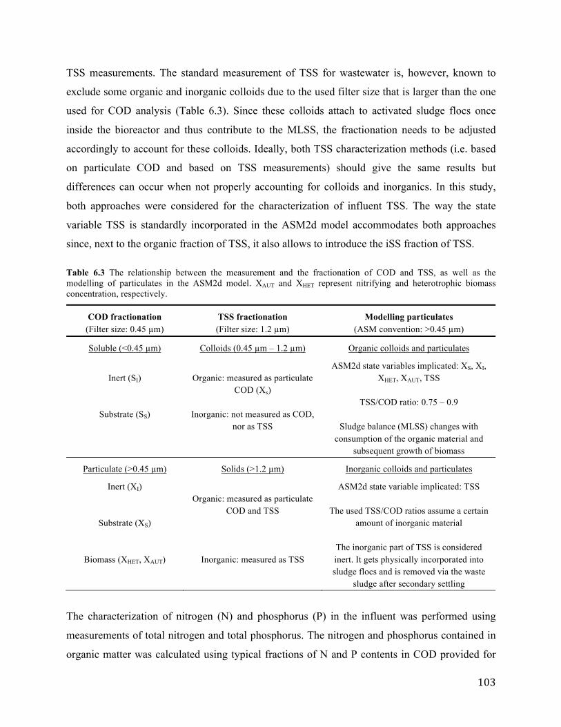
TSS measurements. The standard measurement of TSS for wastewater is, however, known to

exclude some organic and inorganic colloids due to the used filter size that is larger than the one

used for COD analysis (Table 6.3). Since these colloids attach to activated sludge flocs once

inside the bioreactor and thus contribute to the MLSS, the fractionation needs to be adjusted

accordingly to account for these colloids. Ideally, both TSS characterization methods (i.e. based

on particulate COD and based on TSS measurements) should give the same results but

differences can occur when not properly accounting for colloids and inorganics. In this study,

both approaches were considered for the characterization of influent TSS. The way the state

variable TSS is standardly incorporated in the ASM2d model accommodates both approaches

since, next to the organic fraction of TSS, it also allows to introduce the iSS fraction of TSS.

Table 6.3 The relationship between the measurement and the fractionation of COD and TSS, as well as the modelling of particulates in the ASM2d model. XAUT and XHET represent nitrifying and heterotrophic biomass concentration, respectively.

COD fractionation (Filter size: 0.45 µm)

TSS fractionation (Filter size: 1.2 µm)

Modelling particulates (ASM convention: >0.45 µm)

Soluble (<0.45 µm) Colloids (0.45 µm – 1.2 µm) Organic colloids and particulates

Inert (SI)

Substrate (SS)

Organic: measured as particulate

COD (Xs)

Inorganic: not measured as COD, nor as TSS

ASM2d state variables implicated: XS, XI, XHET, XAUT, TSS

TSS/COD ratio: 0.75 – 0.9

Sludge balance (MLSS) changes with

consumption of the organic material and subsequent growth of biomass

Particulate (>0.45 µm) Solids (>1.2 µm) Inorganic colloids and particulates

Inert (XI)

Substrate (XS)

Biomass (XHET, XAUT)

Organic: measured as particulate

COD and TSS

Inorganic: measured as TSS

ASM2d state variable implicated: TSS

The used TSS/COD ratios assume a certain amount of inorganic material

The inorganic part of TSS is considered inert. It gets physically incorporated into sludge flocs and is removed via the waste

sludge after secondary settling

The characterization of nitrogen (N) and phosphorus (P) in the influent was performed using

measurements of total nitrogen and total phosphorus. The nitrogen and phosphorus contained in

organic matter was calculated using typical fractions of N and P contents in COD provided for

ASM2d by Henze et al. (1999) and shown in the supplementary materials (Table 6.6). The

ammonia was then calculated as the difference between the total nitrogen (TKN) available from

the measurements and the calculated nitrogen content in organic matter throughout the year. The

calculated ammonia results were successfully verified over the three days of the sampling

campaign during which measurements of ammonia were available.

As shown in Table 6.2, data for COD and TKN were available at a frequency of one to two

measurements per week for a year. However, to increase the resolution of the model one value

per day is needed for the conventional pollutants. For combined sewers, COD and TKN can be

correlated with the influent flow, and the correlations are used to increase the time resolution of

the characterized influent if frequent flow data are available (Rousseau et al., 2001). However,

analysis of the data for the studied WWTP did not show meaningful correlations between the

flow rate and the aforementioned measurements (not shown), which is likely related to its

separate sewer system. Therefore, the time resolution of the influent measurements was

increased by fitting the less-frequently measured data to a best-fit polynomial function. These

polynomials captured the yearly profile of the measurements and allowed interpolation for daily

values to be used for input generation. The fits are given in the Supplementary Material (Figure

6.6). More detailed diurnal patterns of conventional pollutants in the influent were deemed

unnecessary given the modelling goal. Thus, the achieved conventional pollutant model should

not be evaluated based on sub-daily dynamics.

6.4.6. Simulation approach and calibration

Preliminary simulations were carried out using the default ASM parameters listed by Henze et al.

(2000) and default settler parameters suggested in the COST Simulation Benchmark manual

(Copp, 2002). Each dynamic simulation was preceded by a steady simulation for a period

equivalent to at least three times the SRT (i.e. 20 days) in order to determine the initial

conditions for the dynamic simulation (Rieger et al., 2013).

Model calibration efforts were focused on fitting variables that directly impact the fate of

micropollutants, such as dissolved oxygen concentration, solids concentration and nutrients

concentration. The first step was the calibration of the oxygen mass transfer coefficient (kLa) to

match the measured DO, which was in general observed to be abundant (i.e. average > 5mg/L).

The second step involved achieving a match between the simulated and the measured TSS

concentration at different locations in the activated sludge process, such as the waste sludge (i.e.

WAS TSS), the aeration tank (i.e. MLSS) and the secondary effluent (i.e. Effluent TSS). The

solids balance was first pursued by calibrating the settling parameters. Results of this initial

calibration work could give an indication as to whether adjusting the settling parameters is

sufficient to obtain the correct solids balance, or if, alternatively, characterization of the input

solids is the appropriate approach for achieving the solids balance. The third step involved

achieving an agreement with measured nutrients: NH4 (and its product NO3), as well as COD.

This last step can depend on several biokinetic parameters such as growth rates, decay rates and

substrate affinities. However, for a conventional activated sludge process, these parameters are

relatively well known (Henze et al., 2000), and large calibration efforts should be avoided. That

is because discrepancies between model predictions and measurements that require the

calibration of these parameters may indicate other underlying calibration problems related to the

hydraulic model or the solids balance.

The parameters that correspond to each step were varied using the scenario analysis tool in

WEST software, and the best-fit model was decided upon by visual inspection. While the

simulations were set to provide hourly values of the output variables, the measurements of the

same variables were based on daily flow-proportional samples. Therefore, it was necessary to

calculate the daily flow-average of the simulated results using the equation: ,

where represents the flow-average concentration, and represent the flow rate and the

simulated output concentration at a certain time point “i”. This provided simulated values with

similar time scale as the experimental measurements for the purpose of comparison.

6.5. Results and discussions

The first step towards the calibration of the conventional pollutant model is the characterization

of the influent wastewater. This was followed by calibration of the model for the prediction of

the dissolved oxygen concentration followed by solids concentration, including characterization

of influent solids and finally, model calibration with respect to the nutrient concentrations.

6.5.1. Wastewater characterization

The recorded flow rates throughout the year seemed to be stable due to the mostly separate sewer

system (i.e. with very few combined sewers), which is expected to reduce the seasonal variations

in flow rates due to the seasonal variations in rainfall. The recorded temperatures varied from 15

°C to 22 °C throughout the year. The measured COD concentration trends showed an increase in

winter compared to the summer, which might be due to increased degradation of COD in the

sewers and primary clarifier at the higher temperatures in the summer. It is important to note that

the primary clarifier of this plant has a long retention time of almost 4 hours (Table 6.1), making

that degradation in the clarifier more significant than in typical primary clarifiers. On the other

hand, the incoming ammonia concentrations to the activated sludge unit under study showed no

significant seasonal variation throughout the year. This could be attributed to the absence of

nitrogen removing processes in the mostly anaerobic conditions of a sewer system and primary

clarifier. In addition to ammonia, the TSS profile did not show variation over the one-year

period. The measured TSS values had an average value of 70 g/m3 in the primary effluent, which

corresponds to a TSS reduction of 84% in the primary clarifier. This TSS reduction is larger than

the typical reduction of 40-60% (Office of Water Programs, 1980) in primary clarifiers, likely

because of the chemically enhanced settler that is known to achieve high TSS removal. The

incoming TSS characterization is further discussed in Section 6.5.3 as part of the calibration for

solids.

Table 6.4 summarizes the fractions of the incoming COD obtained over the three days of the

sampling campaign and applied for the whole year. It should be noted that the extra

measurements used for obtaining these fractions over three days in the summer fall on the same

fitted polynomial that describes the data over the full year (i.e. Figure 6.6). This indicates that

there were no special events on these days that could affect the wastewater composition.

Typically, the biodegradable material contained in the primary effluent is predominantly

particulate (i.e. slowly biodegradable material) rather than soluble (Henze et al., 2000); however,

the characterization results shown in Table 6.4 indicated more biodegradable matter in the

soluble phase than in the particulate phase (Ss > XS). This could be attributed to two main factors.

First, the higher TSS reduction known to occur in chemically enhanced primary clarifiers

contributes to the low fraction of particulates in the primary effluent. Second, hydrolysis could

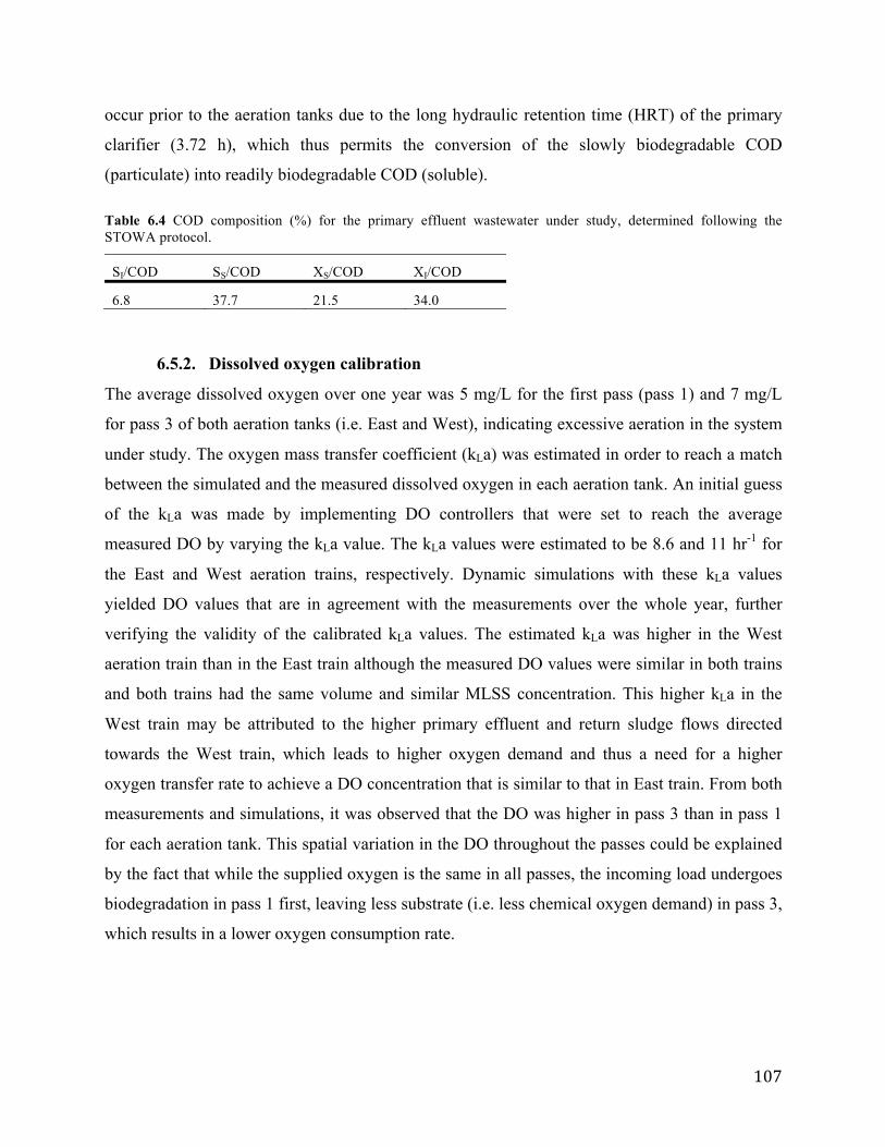
occur prior to the aeration tanks due to the long hydraulic retention time (HRT) of the primary

clarifier (3.72 h), which thus permits the conversion of the slowly biodegradable COD

(particulate) into readily biodegradable COD (soluble).

Table 6.4 COD composition (%) for the primary effluent wastewater under study, determined following the STOWA protocol.

SI/COD SS/COD XS/COD XI/COD

6.8 37.7 21.5 34.0

6.5.2. Dissolved oxygen calibration

The average dissolved oxygen over one year was 5 mg/L for the first pass (pass 1) and 7 mg/L

for pass 3 of both aeration tanks (i.e. East and West), indicating excessive aeration in the system

under study. The oxygen mass transfer coefficient (kLa) was estimated in order to reach a match

between the simulated and the measured dissolved oxygen in each aeration tank. An initial guess

of the kLa was made by implementing DO controllers that were set to reach the average

measured DO by varying the kLa value. The kLa values were estimated to be 8.6 and 11 hr-1 for

the East and West aeration trains, respectively. Dynamic simulations with these kLa values

yielded DO values that are in agreement with the measurements over the whole year, further

verifying the validity of the calibrated kLa values. The estimated kLa was higher in the West

aeration train than in the East train although the measured DO values were similar in both trains

and both trains had the same volume and similar MLSS concentration. This higher kLa in the

West train may be attributed to the higher primary effluent and return sludge flows directed

towards the West train, which leads to higher oxygen demand and thus a need for a higher

oxygen transfer rate to achieve a DO concentration that is similar to that in East train. From both

measurements and simulations, it was observed that the DO was higher in pass 3 than in pass 1

for each aeration tank. This spatial variation in the DO throughout the passes could be explained

by the fact that while the supplied oxygen is the same in all passes, the incoming load undergoes

biodegradation in pass 1 first, leaving less substrate (i.e. less chemical oxygen demand) in pass 3,

which results in a lower oxygen consumption rate.

6.5.3. Solids calibration

Reaching a proper solids balance by achieving a match between the measured and simulated TSS

in aeration tank (i.e. MLSS) and, more importantly, TSS in the waste sludge (i.e. WAS TSS) is

an essential requirement for predicting the fate of micropollutants. This is explained by the fact

that the WAS TSS impacts the extent of micropollutant removal by adsorption, as well as the

SRT that influences the extent of micropollutant biodegradation (Kreuzinger et al., 2004).

6.5.3.1. Initial simulations

For the purpose of initial simulations, the TSS in the influent was characterized based on

particulate COD concentrations according to the typical approach and using typical TSS/COD

ratios suggested by Henze et al. (1999). However, the results obtained using this approach

showed simulated MLSS concentrations that were higher and contained more seasonal variations

throughout the year compared to the measured MLSS that showed no seasonal variation (Figure

6.2(a), Case A). A similar discrepancy between simulation results and measurements was

observed for the TSS in the secondary waste sludge (results not shown). This discrepancy in the

solids balance was concluded to be caused by the mischaracterization of the incoming solids to

the activated sludge system. This was further supported by the fact that manipulating the settler’s

parameters failed to achieve a correct solids balance and to capture the actual WAS TSS and

MLSS concentrations. To remediate the discrepancies in the solids balance and to achieve an

agreement between the simulated and the measured MLSS and WAS TSS concentrations, the

characterization of incoming solids was analysed in more detail.

6.5.3.2. Characterization of incoming solids

As discussed earlier, the COD-based TSS concentration (i.e. input TSS calculated using

TSS/COD conversion factors) showed seasonal variation, similar to the COD, resulting in a

seasonally variable MLSS time series, unlike the measured MLSS profile (Figure 6.2(a)). In

addition, the average simulated MLSS was observed to be higher than the measured MLSS using

the COD-based TSS in the input. In fact, unlike the measured COD, the measured TSS did not

show any seasonal variations throughout the year, indicating that the TSS/COD ratio is not

constant throughout the year. The presence of the CEPT might cause seasonal alterations to the

actual TSS/COD ratio (i.e. caused by changes in the chemical efficiency and solids settling as a

result of temperature variation (Tik & Vanrolleghem, 2012)), indicating that the typical ratios

used for the calculations of the COD-based TSS in the primary effluent (Henze et al., 1999) may

not be valid and that an alternative route for TSS characterization is required. Therefore,

simulations were carried out using the measured TSS as an input, which was found to yield a

simulated MLSS profile that, as desired, did not show seasonal variations, but that was lower

than the measured MLSS and in almost perfect agreement with the measured MLVSS time

series, as shown in Figure 6.2(b). The latter indicated that a fraction of the input suspended solids

was not properly accounted for in the fractionated influent.

Figure 6.2 Measured and predicted MLSS concentrations. The latter was obtained using the Takács model and standard settling parameters: Case A: COD-based TSS in the influent, Case B: Measured TSS in influent, Case C: 1.35 x measured TSS in the influent. The time axis is from July 2013 to June 2014.

As mentioned earlier in Section 6.4.5, the measured TSS does not account for organic and

inorganic colloidal matter, which results in the underestimation of the actual TSS in the influent

(Henze et al., 2000). To remedy this, the TSS at the input was scaled up by a ratio of 1.35, which

was shown to lead to satisfactory predictions of the MLSS in the bioreactors and TSS in the

secondary waste sludge (Figure 6.2(c) and Figure 6.3 respectively). This obtained ratio between

the calibrated and the measured TSS in the input to activated sludge treatment is slightly lower

than that reported by Henze et al. (2000) for an ASM2d model (i.e. 1.5). The lower ratio in the

present study is suggested to be attributed to the presence of the CEPT that may reduce the

colloidal fraction with a higher efficiency than a conventional primary clarifier, requiring a

smaller correction for TSS compared to conventional primary clarification. In fact, it was

previously shown that a well-operated CEPT is capable of almost completely removing colloidal

material (Balmat, 1957; Heukelekian & Balmat, 1959; Ødegaard, 1992; Ødegaard, 2005).

Figure 6.3 Measured and predicted TSS concentrations in waste sludge (WAS TSS) after input solids characterization. The time axis is from July 2013 to June 2014.

6.5.3.3. Calibration with respect to effluent TSS

Once the MLSS and WAS TSS were successfully matched, the settling model was further

calibrated to predict the TSS concentration in the effluent. Predicting the TSS in the secondary

effluent is essential for the subsequent prediction of adsorbed micropollutants in the secondary

effluent stream, as well as to properly calculate the SRT, which determines the micropollutant

biodegradation capacity of the sludge. Both the Takács and the Bürger-Diehl settler models were

tested as shown in Figure 6.4 with the combination of parameter values summarized in Table 6.5.

Although the Bürger-Diehl model allows for including the compression and the dispersion

phenomena, the low measured sludge volume index (SVI) values (i.e. average of 58 mL/g)

indicated sludge with very good settling and thickening properties, making it reasonable to

assume that compression settling does not play a significant role in the system under study.

Accounting for dispersion, which is another phenomenon included in the Bürger-Diehl model

and expressed as a function of the input flow rate, was deemed unnecessary. This is explained by

the absence of significant flow variations in the input to the activated sludge unit, due to the

presence of a separate sewer system. Using the Takács model with the default values for the

settling parameters, the simulated TSS in the effluent was observed to be much higher than the

measured one, as shown in Figure 6.4 (Takács A). Lowering the simulated effluent TSS to match

the measured profile was achieved by increasing the rP parameter (i.e. from 2.86 to 7 L/g) and

lowering the f-ns parameter (i.e. from 2.28 to 0), as shown in Figure 6.4 (Takács B). The

observed impact of varying these parameters is explained by the fact that lowering the f-ns leads

to a lower fraction of non-settleable solids decreasing the effluent TSS, while a higher rP value

increases the settling velocity and, therefore, decreases the TSS in the effluent.

On the other hand, when using the Bürger-Diehl model, the simulated TSS profile is lower than

the profile obtained using the Takács model for default parameter values (Bürger-Diehl A vs.

Takács A, Figure 6.4). Even though both compression and dispersion of the Bürger-Diehl model

were turned off, the better prediction is explained by the existence of two extra top layers in the

Bürger-Diehl model that account for the flux over the outlet boundary. Using a larger number of

layers in the Bürger-Diehl model (30 layers) as compared to the 10-layer Takács model was also

anticipated to result in more representative effluent solids concentrations by diminishing

numerical dispersion. Since an agreement between the measured and simulated effluent TSS was

not yet achieved using default parameters, the rP parameter was adjusted to 5 L/g, which resulted

in a match between the measurements and simulations (Figure 6.4, Bürger-Diehl B). This

indicated that a less extensive calibration was required for the Bürger-Diehl model (i.e. only one

parameter) compared to the Takács model in order to match the effluent TSS measurements.

This justified the use of this model for the settler rather than the Takács model. The fit of the

final model for effluent TSS is shown in Figure 6.4 (Case Bürger-Diehl B).

Figure 6.4 Comparison of predicted effluent TSS concentrations obtained using the Takács and Bürger-Diehl settler models with different parameters (Table 6.5). The time axis is from July 2013 to June.

Table 6.5 Parameter values tested for each of the settler models (Takács and Bürger-Diehl). Results corresponding to these cases are shown in Figure 6.4.

Case rH (L/g) rP (L/g) f-ns (%) Takacs A (default) 0.576 2.86 2.28 Takacs B 0.576 7 0Bürger Diehl A 0.576 2.86 2.28 Bürger Diehl B 0.576 5 2.28

6.5.4. Nutrients calibration

As shown in Figure 6.5, once the model was able to accurately predict the solids balance, the

effluent nutrient and COD predictions were on average in good agreement with the

measurements, keeping in mind the goal of the modelling, without performing any further

calibration of biokinetic parameters. In particular, the slightly reduced nitrification by the end of

the winter (i.e. between days 200 and 300 on Figure 6.5) was well captured by the calibrated

model. This emphasizes the importance of obtaining the correct hydraulic model and solids

balance before modifying the biokinetic parameters. The simulated COD (Figure 6.5) did not

show the same fluctuations as the measured values but the general profile matched the collected

data. The high nitrate values observed in the secondary effluent of the studied treatment plant

(Figure 6.5) can be explained by the high DO in the treatment lines (well above 2 mg/L)

throughout the year, rendering it impossible for denitrification to occur. The measured nitrite

concentrations in the secondary effluent were <0.5 mg/L, except during the winter where it rose

slightly (not shown), indicating that the activated sludge plant under study is a fully nitrifying

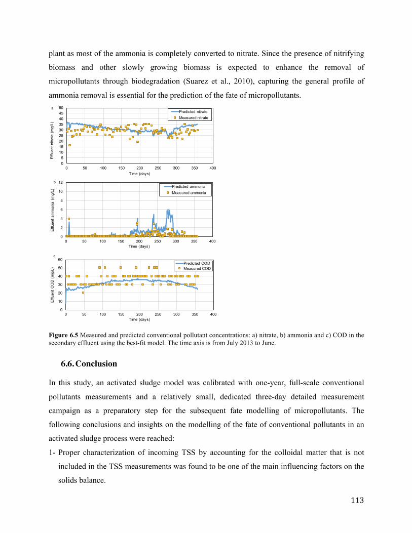
plant as most of the ammonia is completely converted to nitrate. Since the presence of nitrifying

biomass and other slowly growing biomass is expected to enhance the removal of

micropollutants through biodegradation (Suarez et al., 2010), capturing the general profile of

ammonia removal is essential for the prediction of the fate of micropollutants.

Figure 6.5 Measured and predicted conventional pollutant concentrations: a) nitrate, b) ammonia and c) COD in the secondary effluent using the best-fit model. The time axis is from July 2013 to June.

6.6. Conclusion

In this study, an activated sludge model was calibrated with one-year, full-scale conventional

pollutants measurements and a relatively small, dedicated three-day detailed measurement

campaign as a preparatory step for the subsequent fate modelling of micropollutants. The

following conclusions and insights on the modelling of the fate of conventional pollutants in an

activated sludge process were reached:

1- Proper characterization of incoming TSS by accounting for the colloidal matter that is not

included in the TSS measurements was found to be one of the main influencing factors on the

solids balance.

2- The chemically enhanced primary treatment was considered to seasonally influence the

particulate composition of the primary effluent, requiring special considerations during the

characterization of the incoming TSS fraction to the activated sludge unit.

3- The Bürger-Diehl model for the secondary settler resulted in improved calibration of the

effluent TSS compared to the Takács model, which is related to the inclusion of additional

layers to model the outlet boundaries.

4- Careful calibration of the solids balance through detailed influent characterization and

appropriate selection of the settler model allowed the measured nutrient profiles in the

effluent to be captured by the model using default ASM parameters.

The routine measurements available from the WWTP based on 24-h composite samples were

proven to be sufficient to successfully model the general yearly profiles of WAS TSS, effluent

TSS, DO and nutrients. Since these variables are linked to the main removal processes of

micropollutants (i.e. through SRT, aeration and solids balance), it is shown that the measurement

effort and resources required for the conventional modelling that is performed as a preliminary

step for calibration of the micropollutant model can remain limited.

6.7. Acknowledgements

The authors thank the staff at the Guelph WWTP for their help in providing the data. We

gratefully acknowledge the McGill Engineering Doctoral Award for supporting Zeina Baalbaki.

Funding for this study was provided by a research grant to Viviane Yargeau (PI) and colleagues

(Chris Metcalfe and Peter Vanrolleghem) from the Natural Sciences and Engineering Research

Council (NSERC) of Canada through the Strategic Grants Program (430646-2012). Peter

Vanrolleghem holds the Canada Research Chair on Water Quality Modelling.

6.8. Supplementary material:

Table 6.6 Organic nitrogen and phosphorus content in the fractions constituting organic matter (Henze et al., 2000). Fraction in COD SF

a SAa SI Xs XI

Nitrogen 0.03 0.01 0 0.04 0.02 Phosphorus 0.01 0 0 0.01 0.01 SF: fermentable organic matter (soluble), SF: Acetate organic matter and other fermentation products (soluble).

SF+SA=SS

Figure 6.6 Polynomial fit of measured COD (upper) and TKN (lower) in the primary effluent. Time axis is from

July 2013 to June 2014.

7. PREDICTING THE FATE OF MICROPOLLUTANTS DURING WASTEWATER TREATMENT: CALIBRATION AND SENSITIVITY ANALYSIS 7.1. Preface

This manuscript addresses the last objective of this PhD project i.e. to predict the fate of CECs in

activated sludge treatment and determine the most influential model parameters. Previous

dynamic models have been developed to predict the fate of some CECs in WWTPs, but no

information is available in the literature on the sensitivity of these micropollutant fate models to

the calibrated model parameters or on the uncertainty of the calibrated parameters.

In this manuscript, the focus was on four of the target CECs of Chapter 5 (i.e. caffeine,

ibuprofen, androstenedione and triclosan) which belong to different classes of contaminants and

are known to have different fate behaviours in activated sludge processes. Full-scale

measurements of these CECs in activated sludge treatment obtained in Chapter 5 were used for

calibration of the fate model. The model calibrated with respect to the measured dissolved

oxygen, solids and nutrients in Chapter 6 was used in the current chapter as a basis for prediction

of the fate of CECs. While most studies in the literature ignored the fate processes in the

secondary clarifier, in the present manuscript these were included and the effect of ignoring them

was investigated. Calibration was performed by minimizing the errors between simulation results

and measurements of CEC concentrations in aqueous and particulate output streams fulfilling

one aspect of the research objectives i.e. to calibrate the micropollutant fate model.

This manuscript confirmed the basic hypothesis that the fate of the target CECs in activated

sludge could be well represented by mechanistic equations describing the biodegradation and

sorption fate processes. Calibration yielded output CEC concentrations that are in agreement

with measurements in both soluble and particulate phases of the output streams from the

activated sludge unit. Ignoring the MP fate processes taking place in the secondary clarifier was

observed to bias the concentration of caffeine in the settler’s underflow, indicating that some

biodegradation of caffeine takes place in the settler. One of the objectives of this work was to

determine the most influential parameters on the model output, and this study demonstrated that

while the fate model is highly sensitive to some parameters, others had no influence on the

model fit implying that calibration of these parameters is not necessary. This study also provided

evidence that the set of the most influential parameters is dependent upon the nature of the CEC

and the corresponding major fate processes affecting its fate. Further, using dynamic sensitivity

analysis, the model’s sensitivity to the calibrated parameters was demonstrated to be time-

dependent, which was associated to time-dependent input CEC concentration and may help to

plan future measurement campaigns.

This manuscript has been submitted for publication in Science of the Total Environment.

Predicting the fate of micropollutants during wastewater treatment: calibration and sensitivity analysis Zeina Baalbaki a, Elena Torfs b*, Viviane Yargeau a, Peter A. Vanrolleghem b

a Department of Chemical Engineering, McGill University, 3610 University St., Montreal, QC, H3A 0C5 b modelEAU, Département de génie civil et de génie des eaux, Université Laval, 1065 Avenue de la médecine, Québec City, QC, G1V 0A6 * elena.torfs.1@ulaval.ca

7.2. Abstract

The presence of micropollutants in the environment and their toxic impacts on the aquatic

environment have raised concern about their inefficient removal in wastewater treatment plants.

In this study, the fate of micropollutants of four different classes was simulated in a conventional

activated sludge plant using a bioreactor micropollutant fate model coupled to a settler model.

The latter was based on the Bürger-Diehl model extended for the first time to include

micropollutant fate processes. Calibration of model parameters was completed by matching

modelling results with full-scale measurements (i.e. including aqueous and particulate phase

concentrations of micropollutants) obtained from a 4-day sampling campaign. Modelling results

showed that further biodegradation takes place in the sludge blanket of the settler for the highly

biodegradable caffeine, underlining the need for a reactive settler model for accurate fate

prediction. The adopted Monte Carlo based calibration approach also provided an overview of

the model’s global sensitivity to the parameters and showed that for each micropollutant a

different set of one or more parameters had a significant impact on the model fit. The set of

influential parameters could be related to dominant fate processes of each CEC justifying the

selection of parameter subsets for model calibration. A dynamic local sensitivity analysis was

also performed with the calibrated parameters. This analysis supported the conclusions from the

global sensitivity analysis and linked the dynamic changes in sensitivity to the time-dependent

input micropollutant concentrations, providing guidance for future sampling campaigns. This

study expands the understanding of micropollutant fate models when applied to different

micropollutants, in terms of global and local sensitivity to model parameters, as well as the

identifiability of the parameters.

Keywords: Contaminants of emerging concern, Biological treatment, Activated sludge treatment,

Dynamic sensitivity, Fate model

7.3. Introduction

The presence of pharmaceuticals and personal care products (PPCPs), as well as hormones, in

the environment was proven to cause adverse effects on aquatic life raising concern about their

insufficient removal from wastewater (Gay et al., 2016; Kidd et al., 2007; Purdom et al., 1994).

The two major processes influencing the fate of micropollutants (MPs) during activated sludge

treatment are biodegradation and sorption that act at different degrees on MPs with different

characteristics (Joss et al., 2006; Radjenović et al., 2009b; Ternes et al., 2004b). Hence, although

most of the emphasis in activated sludge mathematical modelling has been placed on

conventional pollutants, some mathematical models were also developed to describe the fate and

discharge of MPs in activated sludge systems and proposed as a cost-effective tool for risk

assessment (Cowan et al., 1993; Plósz et al., 2012; Urase & Kikuta, 2005; Vezzaro et al., 2014).

Since the fate of MPs is influenced by the fate of conventional pollutants (e.g. solids that affect

the sorption and biodegradation of micropollutants), simultaneous modelling of conventional and

micropollutants was made possible by extending the well-known Activated Sludge Models

(ASMs) developed many years ago (Henze et al., 1987; Henze et al., 1999). The most notable

examples of models tackling both conventional pollutants and MPs are the ASM-X model (Plósz

et al., 2012; Plósz et al., 2010) and another more recent model based on the ASM2d model

(Vezzaro et al., 2014). The majority of MP fate studies in activated sludge focused their efforts

on the modelling of the removal in bioreactors and considered the MP fate processes taking place

in the secondary clarifier as insignificant (Cloutier et al., 2008; Plósz et al., 2010). However, one

study by Vezzaro et al. (2014) extended the Takács settling model (Takács et al., 1991) to

include the MP fate processes in the clarifier.

Previous efforts were made to calibrate the model parameters that describe the kinetics and

equilibrium of biodegradation and sorption of several MPs (Cloutier et al., 2008; Cowan et al.,

1993; Pomiès et al., 2013), with only few studies focusing on PPCPs and hormones (Plósz et al.,

2012; Plósz et al., 2010; Urase & Kikuta, 2005). Calibration often focused on the kinetics of

biodegradation only, assuming that sorption occurs much more rapidly (Abegglen et al., 2009;

Suarez et al., 2010; Urase & Kikuta, 2005). As a result, full-scale micropollutant concentration

measurements for model parameter calibration focused mostly on the aqueous phase in previous

studies without measuring the MP load partitioned onto sludge (Joss et al., 2004; Plósz et al.,

2012; Xue et al., 2010). Moreover, the large uncertainty on the calibrated parameters reported in

the literature was identified as a major gap in the field of micropollutant modelling in WWTPs, a

factor that is aggravated by the lack of knowledge on the sensitivity of the MP fate models to

their parameters (Pomiès et al., 2013). This leaves the model users unsure about the degree of

confidence in the parameters values reported in the literature.

In the present study, a MP fate model based on ASM2d (bioreactor) was further modified and

coupled to a reactive settler model extended for the first time from the Bürger-Diehl settler

model which itself incorporates the latest important advancements in the field of secondary

settler modelling (Bürger et al., 2012). The scope of the current paper was to calibrate the MP

model’s parameters using MP concentration measurements collected from a 4-day sampling

campaign at a full-scale WWTP, which was meant to be feasible in terms of efforts and

resources supplied by the utility running the plant. Given the chronic nature of the impacts of the

studied CECs, sub-daily variations were not deemed of importance for this study, and only the

24-h average load was considered for sampling. Samples were collected under dry weather

conditions, since that is when surface water bodies are expected to be the most sensitive to

wastewater discharges as a result of the limited dilution. A model that was previously calibrated

with respect to conventional pollutants using one-year data was used as a starting point for the

current MP calibration. The MPs investigated in the present study included a hormone

(androstenedione), a pharmaceutical (ibuprofen), an antibacterial agent (triclosan) and a nervous

stimulant (caffeine). Ibuprofen, triclosan and caffeine were selected based on their high detection

frequency in wastewater effluents (Dickenson et al., 2011), while little data is available regarding

the levels and fate of androstenedione (Baalbaki et al., 2016; Esperanza et al., 2007). The target

MPs were also previously observed to be influenced by sorption and biodegradation fate

processes to variable extents in WWTPs (Baalbaki et al., 2016), while volatilization is not

considered as significant (Struijs et al., 1991; Virkutyte et al., 2010). For sorption, both the

kinetics and the equilibrium equations were considered in the bioreactor and settler models.

Sensitivity analysis was performed to explore the impact of the MP fate model parameters on

each of the fitted variables, in relation to the input dynamics. Prior to calibrating the model for

micropollutant fate, the hydraulic model of the WWTP was identified and the activated sludge

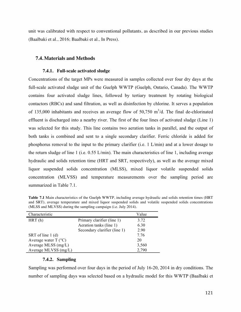
unit was calibrated with respect to conventional pollutants, as described in our previous studies

(Baalbaki et al., 2016; Baalbaki et al., In Press).

7.4. Materials and Methods

7.4.1. Full-scale activated sludge Concentrations of the target MPs were measured in samples collected over four dry days at the

full-scale activated sludge unit of the Guelph WWTP (Guelph, Ontario, Canada). The WWTP

contains four activated sludge lines, followed by tertiary treatment by rotating biological

contactors (RBCs) and sand filtration, as well as disinfection by chlorine. It serves a population

of 135,000 inhabitants and receives an average flow of 50,750 m3/d. The final de-chlorinated

effluent is discharged into a nearby river. The first of the four lines of activated sludge (Line 1)

was selected for this study. This line contains two aeration tanks in parallel, and the output of

both tanks is combined and sent to a single secondary clarifier. Ferric chloride is added for

phosphorus removal to the input to the primary clarifier (i.e. 1 L/min) and at a lower dosage to

the return sludge of line 1 (i.e. 0.55 L/min). The main characteristics of line 1, including average

hydraulic and solids retention time (HRT and SRT, respectively), as well as the average mixed

liquor suspended solids concentration (MLSS), mixed liquor volatile suspended solids

concentration (MLVSS) and temperature measurements over the sampling period are

summarized in Table 7.1.

Table 7.1 Main characteristics of the Guelph WWTP, including average hydraulic and solids retention times (HRT and SRT), average temperature and mixed liquor suspended solids and volatile suspended solids concentrations (MLSS and MLVSS) during the sampling campaign (i.e. July 2014). Characteristic Value HRT (h) Primary clarifier (line 1) 3.72

Aeration tanks (line 1) 6.30 Secondary clarifier (line 1) 2.90

SRT of line 1 (d) 7.76 Average water T (°C) 20 Average MLSS (mg/L) 3,560 Average MLVSS (mg/L) 2,790

7.4.2. Sampling Sampling was performed over four days in the period of July 16-20, 2014 in dry conditions. The

number of sampling days was selected based on a hydraulic model for this WWTP (Baalbaki et

al., 2016). As shown in Figure 7.1, samples were collected from the effluent of the primary

clarifier or primary effluent (PE), the effluent of the aeration tanks (AE), the effluent of the

secondary clarifier (SE), as well as from the secondary waste sludge at the underflow of the

secondary clarifier (WAS) and from the sludge of the primary clarifier (not shown in Figure 7.1).

Samples from the PE and SE were collected as 24-h composite samples using onsite Hach Sigma samplers, where the samples were refrigerated at 4°C until retrieved (daily). Due to the absence

of an onsite sampler in the AE location, 24-h composite samples from this stream were obtained

using ISCO 6712 samplers (Avensys, St-Laurent, QC, Canada) equipped with 24 bottles and

packed with ice (replaced daily). Waste activated Sludge samples were collected as grab samples

on each of the four days. All collected samples were transferred into 1-L Nalgene certified pre-

cleaned amber bottles (Fisher Scientific) at the end of each day of sampling, stored at -20 °C and

kept frozen until extracted.

Figure 7.1 Schematic of the investigated full-scale activated sludge unit. Sampling locations are indicated with a cross sign (PE: primary effluent, AE: aeration effluent, SE: secondary effluent, WAS: waste activated sludge) and the corresponding measurements taken (SMP and XMP indicate measurement of the micropollutant concentration in aqueous and particulate phases, respectively).

7.4.3. Sample preparation The four target micropollutants extracted from the wastewater and biosolids samples, as well as

information on their respective internal standards and suppliers, are listed in Table 7.2. The

aqueous samples from the PE, AE and SE locations were filtered using 1-μm glass-fiber filters

(Fisher Scientific). The filtered samples (100 mL for PE and 200 mL for AE and SE) were

spiked with internal standards to account for the extraction recovery and matrix effects and then

subjected to solid-phase extraction (SPE). The cartridges used for extraction were the Oasis

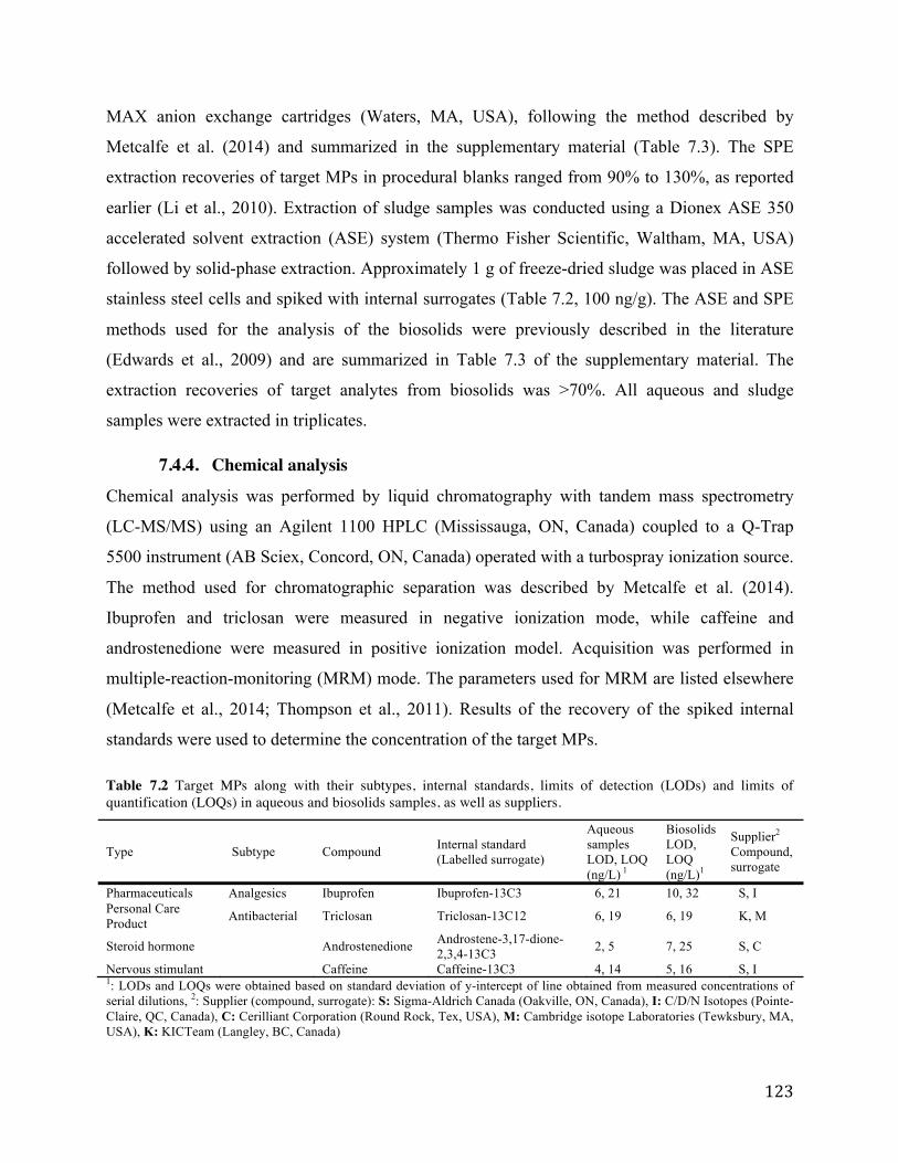
MAX anion exchange cartridges (Waters, MA, USA), following the method described by

Metcalfe et al. (2014) and summarized in the supplementary material (Table 7.3). The SPE

extraction recoveries of target MPs in procedural blanks ranged from 90% to 130%, as reported

earlier (Li et al., 2010). Extraction of sludge samples was conducted using a Dionex ASE 350

accelerated solvent extraction (ASE) system (Thermo Fisher Scientific, Waltham, MA, USA)

followed by solid-phase extraction. Approximately 1 g of freeze-dried sludge was placed in ASE

stainless steel cells and spiked with internal surrogates (Table 7.2, 100 ng/g). The ASE and SPE

methods used for the analysis of the biosolids were previously described in the literature

(Edwards et al., 2009) and are summarized in Table 7.3 of the supplementary material. The

extraction recoveries of target analytes from biosolids was >70%. All aqueous and sludge

samples were extracted in triplicates.

7.4.4. Chemical analysis Chemical analysis was performed by liquid chromatography with tandem mass spectrometry

(LC-MS/MS) using an Agilent 1100 HPLC (Mississauga, ON, Canada) coupled to a Q-Trap

5500 instrument (AB Sciex, Concord, ON, Canada) operated with a turbospray ionization source.

The method used for chromatographic separation was described by Metcalfe et al. (2014).

Ibuprofen and triclosan were measured in negative ionization mode, while caffeine and

androstenedione were measured in positive ionization model. Acquisition was performed in

multiple-reaction-monitoring (MRM) mode. The parameters used for MRM are listed elsewhere

(Metcalfe et al., 2014; Thompson et al., 2011). Results of the recovery of the spiked internal

standards were used to determine the concentration of the target MPs.

Table 7.2 Target MPs along with their subtypes, internal standards, limits of detection (LODs) and limits of quantification (LOQs) in aqueous and biosolids samples, as well as suppliers.

Type Subtype Compound Internal standard (Labelled surrogate)

Aqueous samples LOD, LOQ (ng/L) 1

Biosolids LOD, LOQ (ng/L)1

Supplier2 Compound, surrogate

Pharmaceuticals Analgesics Ibuprofen Ibuprofen-13C3 6, 21 10, 32 S, I Personal Care Product Antibacterial Triclosan Triclosan-13C12 6, 19 6, 19 K, M

Steroid hormone Androstenedione Androstene-3,17-dione-2,3,4-13C3 2, 5 7, 25 S, C

Nervous stimulant Caffeine Caffeine-13C3 4, 14 5, 16 S, I 1: LODs and LOQs were obtained based on standard deviation of y-intercept of line obtained from measured concentrations of serial dilutions, 2: Supplier (compound, surrogate): S: Sigma-Aldrich Canada (Oakville, ON, Canada), I: C/D/N Isotopes (Pointe-Claire, QC, Canada), C: Cerilliant Corporation (Round Rock, Tex, USA), M: Cambridge isotope Laboratories (Tewksbury, MA, USA), K: KICTeam (Langley, BC, Canada)

7.4.5. Modelling and simulations The residence time and consequent removal of micropollutants in the WWTP is impacted by the

hydrodynamics of treatment units (Majewsky et al., 2011; Ort et al., 2010). Hence, prior to

modelling the fate of MPs, a hydraulic model of the activated sludge process under study was

created using measurements of the wastewater’s electrical conductivity as a tracer. The optimum

hydraulic model consisted of three aeration tanks in series and one secondary clarifier, which is

described in more details elsewhere (Baalbaki et al., 2016). A detailed calibration of the aeration

and settler model parameters, as well as characterization of input chemical oxygen demand and

suspended solids were performed using one-year measurements of dissolved oxygen, solids and

nutrients at different locations of the studied activated sludge unit (Baalbaki et al., In Press).

Briefly, the calibration procedure aimed at predicting the concentration of biomass, as well as the

solids retention time that is known to affect the diversity of the biomass (Saikaly & Oerther,

2004). The concentration and the diversity of biomass are both expected to have an important

influence on the rate of biodegradation of MPs (Kreuzinger et al., 2004; Suarez et al., 2010). The

calibration performed by Baalbaki et al. (In Press) also aimed at predicting the solids

concentration in the waste stream, which influences the extent of MP removal through

adsorption. Compared to the Takács model, the Bürger-Diehl settling model was found to

provide a better description of the suspended solids balance of the system that plays a key role in

sorption as well as biodegradation of micropollutants. Following proper calibration of the solids

balance, the standard ASM kinetic parameters provided a satisfactory fit to the measurements of

nutrients. High dissolved oxygen was observed in the aeration tanks, indicating a relatively high

oxygen transfer rate parameter, kLa. Further details on the calibration procedure are described

elsewhere (Baalbaki et al., In Press).

All model simulations were performed in the software WEST (MIKE by DHI, Denmark). The

variable-coefficient ODE (i.e. VODE) integrator available in WEST was used with a tolerance of

10-8 for its efficient run time. Processes describing the fate of MPs were included in the

bioreactor model based on the extended bioreactor model library that was first developed by

Vezzaro et al. (2014). The Bürger-Diehl settling model (Bürger et al., 2012) was extended to

include the processes determining the fate of micropollutants (i.e. biodegradation and sorption).

The specific modifications are further elaborated upon in Section 7.5.2 of the discussion. The

modified bioreactor and extended settler models were coupled.

All dynamic simulations were preceded by steady-state simulations over 23 days (i.e. 3xSRT) in

order to obtain a good estimate of the initial conditions of solids concentration in different

locations of the activated sludge unit. Also, to obtain realistic initial conditions of micropollutant

concentrations, dynamic simulations were performed over a period of time starting a few days

before the first day of sampling and assuming that the micropollutant concentrations were similar

to the measured ones. The input to the model (i.e. primary effluent) consisted of the following

measured time series: flow rates, measurements of conventional pollutants, such as TSS,

ammonia and COD, as well as the incoming concentration of the micropollutants in dissolved

and particulate phases. The latter was obtained from analysis of the collected primary sludge.

7.4.6. Model results analysis The model output variables considered are the soluble micropolutant concentration in the

effluent from the aeration tank and secondary clarifier (i.e. SMP-AE and SMP-SE, respectively), as

well as the particulate micropollutant concentration in the waste sludge (i.e. XMP-WAS), as

shown in Figure 7.1. Calibration of model parameters was carried out using a Monte Carlo based

approach with the scenario analysis tool available in WEST, similar to the approach suggested

by Sin et al. (2008). For each parameter, a number of discrete values were defined over a broad

range of parameter values that were based on literature findings, and simulations were performed

for all possible parameter combinations. Subsequently, the goodness of fit for each simulation

was determined by the chi-square ( criterion, as proposed by Dochain and Vanrolleghem

(2001) and expressed in Eq. 7.1, where and represent the predicted and the measured

variable value, respectively at time point and is the standard deviation of the measurements

at time point .

(7.1)

All measurement values (i.e. soluble and particulate micropollutant concentrations) with their

corresponding simulated values were considered for the calculation of in Eq. 7.1. The chi-

square error was used to quantify the degree of mismatch between the results from simulations

and measurements, since it accounts for measurement uncertainty through the standard

deviations obtained from lab replicates for each of the four days. In order to compare the

simulated profiles with the measured ones for error calculations, the simulated profiles were

converted into a similar time scale by calculating the average daily values (flow-average or time-

average), since measurements were based on time-proportional and flow-proportional samples at

the AE and SE locations, respectively. The optimal parameter set was determined from the

simulation with the lowest value. Moreover, by studying the evolution of values over the

tested parameter intervals, conclusions could be drawn on the model fit’s global sensitivity to the

parameters, as well as the identifiability of each parameter (i.e. the existence of a unique small

range of parameter values that minimize the ). In addition to the criterion, the two-sample t-

test with a confidence level of 95% was performed to verify the capability of the best-fit model

to well predict the average micropollutant concentration in the particulate phase in the waste

sludge.

Local sensitivity analysis around the optimal parameter values was carried out in the WEST

software in order to understand the dynamic effect of small variations in the model parameters

on the three model output variables. In theory, the relative sensitivity is determined by Eq. 7.2 in

discrete form, where represents the time, the variable and the input parameter, which is

varied systematically by (perturbation). Therefore, the output of the sensitivity analysis

conveys a message about the percentage change in the output variable resulting from a

theoretical 100% change in the parameter, even though the actual perturbation is significantly

lower than 100%.

(7.2)

7.5. Results and discussion

7.5.1. Observed concentrations and removals In the influent to the activated sludge process, triclosan and androstenedione were observed at

average concentrations of 132 and 65 ng/L, respectively. The widespread analgesic ibuprofen

and the stimulant caffeine present in many beverages entered at higher average concentrations of

1.68 μg/L and 25.3 μg/L, respectively. As observed in the current sampling campaign and

reported in previous work (Baalbaki et al., 2016), the removal of ibuprofen and caffeine by the

activated sludge unit under study was 99% and 94%, respectively. This high removal efficiency

is in good agreement with previous literature (Behera et al., 2011; Clara et al., 2005b;

Radjenović et al., 2009b). Triclosan had a removal of 72 %, also consistent with previous

observations (Behera et al., 2011), while androstenedione was removed at a lower efficiency of

33%. Ibuprofen and androstenedione had an average particulate concentration in the secondary

waste sludge of 39 ng/g and 38 ng/g, respectively. On the other hand, due to its higher input

concentration, caffeine was observed at a high concentration (i.e. 776 ng/g) in secondary waste

sludge. For triclosan, the measured particulate concentration in waste sludge was 1334 ng/g,

which can be attributed to its known hydrophobicity (Petrie et al., 2014). These four MPs were

thus selected for the modelling study based on the diversity observed in their biodegradation and

sorption tendency, as reported in the literature and indicated by experimental results of the

current study. This variability in the fate allows for a more comprehensive exploration of MP

fate model calibration and sensitivity analysis for variable combinations of parameter values.

7.5.2. Model structure The processes accounted for in the model are biological degradation and sorption, since these

were suggested to be the most significant processes for the target MPs (Andersen et al., 2005;

Joss et al., 2006; Ternes et al., 2004b). For a completely mixed unit with constant volume the

micropollutant soluble concentration dynamics are expressed by Eq. 7.3 taking into account the

incoming and outgoing MP load, as well as sorption and biodegradation processes. Given the

presence of ample oxygen (constantly >2.5 mg/l) in the activated sludge system under study (i.e.

above the limit that ensures the absence of anoxic zones), only aerobic biodegradation was

considered. The biodegradation pseudo first-order kinetic equation in the model by Vezzaro et al.

(2014) where the biomass is assumed to be constant was modified to include the effect of

temporal variations in the active biomass concentration, as shown in Eq. 7.4. The active biomass

concentration is calculated by the model as the sum of the concentrations of the following

particulate ASM2d model components: heterotrophic (XOHO), autotrophic (XAOO) and phosphate

accumulating organisms (XPAO). The concentrations of these components composing the biomass

are predicted by the calibrated conventional pollutant model (Baalbaki et al., In Press) that is

used in the present study. A Monod-type substrate saturation kinetics was not deemed necessary

due to the generally low concentrations of micropollutants, as well as the fact that the first-order

kinetic equation was proven to yield satisfactory predictions for micropollutants (Namkung &

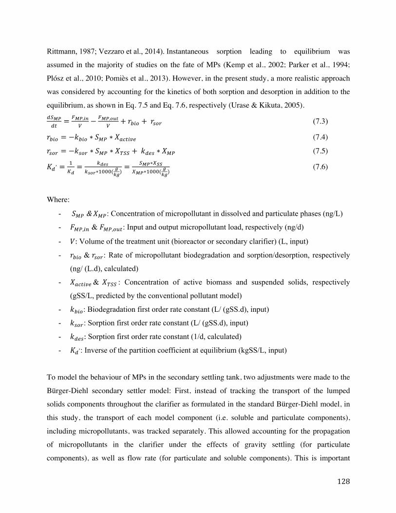
Rittmann, 1987; Vezzaro et al., 2014). Instantaneous sorption leading to equilibrium was

assumed in the majority of studies on the fate of MPs (Kemp et al., 2002; Parker et al., 1994;

Plósz et al., 2010; Pomiès et al., 2013). However, in the present study, a more realistic approach

was considered by accounting for the kinetics of both sorption and desorption in addition to the

equilibrium, as shown in Eq. 7.5 and Eq. 7.6, respectively (Urase & Kikuta, 2005).

(7.3)

(7.4)

(7.5)

(7.6)

Where:

- : Concentration of micropollutant in dissolved and particulate phases (ng/L)

- & : Input and output micropollutant load, respectively (ng/d)

- Volume of the treatment unit (bioreactor or secondary clarifier) (L, input)

- & : Rate of micropollutant biodegradation and sorption/desorption, respectively

(ng/ (L.d), calculated)

- & : Concentration of active biomass and suspended solids, respectively

(gSS/L, predicted by the conventional pollutant model)

- : Biodegradation first order rate constant (L/ (gSS.d), input)

- : Sorption first order rate constant (L/ (gSS.d), input)

- Sorption first order rate constant (1/d, calculated)

- : Inverse of the partition coefficient at equilibrium (kgSS/L, input)

To model the behaviour of MPs in the secondary settling tank, two adjustments were made to the

Bürger-Diehl secondary settler model: First, instead of tracking the transport of the lumped

solids components throughout the clarifier as formulated in the standard Bürger-Diehl model, in

this study, the transport of each model component (i.e. soluble and particulate components),

including micropollutants, was tracked separately. This allowed accounting for the propagation

of micropollutants in the clarifier under the effects of gravity settling (for particulate

components), as well as flow rate (for particulate and soluble components). This is important

since inaccurate representation of the propagation of the soluble and particulate organics within

the clarifier was proven to cause a bias in their concentration in the output sludge that is partially

recycled back (Jeppsson & Diehl, 1996).

The second adjustment was the inclusion of the fate processes (i.e. biodegradation and sorption)

acting on micropollutants in the secondary clarifier. Almost all of the previous studies on MP

fate modelling in activated sludge assumed that removal of micropollutants in the secondary

clarifier is negligible. Figure 7.2 demonstrates that removal processes in the secondary clarifier

can potentially be of importance. Although ignoring biodegradation in the settler does not impact

the MP concentration in the clarifier’s supernatant, it increases the average soluble concentration

of micropollutants in the waste sludge by more than 100% (Figure 7.2(a)). The target

micropollutant caffeine, represented in Figure 7.2, is known to biodegrade extensively, as

discussed earlier, indicating that the high biomass concentration at the bottom of the settler

allows for significant biodegradation to take place (Eq. 7.4). This result is particularly relevant

since, for the system under study, the model predicted only 4% of the total solids mass to be

present in the secondary clarifier which can be explained by the good settling characteristics of

the sludge (i.e. low SVI with an average of 58 mL/g). Consequently, for other activated sludge

systems operating at high sludge blanket and thus containing a higher percentage of solids in the

secondary clarifier, the micropollutant biodegradation process in the secondary clarifier could be

even more significant. Accurate prediction of the micropollutant load in the underflow of the

settler by accounting for the MP biodegradation is particularly important when modelling the

overall fate of MPs in the entire WWTP as the underflow is often partially recycled back to the

head works after treatment, increasing the load of the MP to the WWTP. In contrast, in the upper

region of the settler, the biomass is present at low concentration, which explains the observation

that the simulated concentration of caffeine in the supernatant was unaffected by the inclusion or

exclusion of the biodegradation reactions (Figure 7.2(b)). This difference in the extent of

biodegradation throughout the settler results in spatial variation in the soluble and particulate

micropollutant concentrations across the settler that is overlooked in non-reactive settler models.

Figure 7.2 Predicted soluble caffeine concentration in the two secondary clarifier outputs: a) secondary waste sludge and b) secondary effluent, accounting for both sorption and biodegradation (Ads+ bio), only sorption (Ads) or none of the fate processes (None).

7.5.3. Impact of individual model parameters The behaviour of the model and the interaction between the different processes (i.e.

biodegradation Eq. 7.4 and adsorption Eq. 7.5) are illustrated in Figure 7.3 by changing process

parameters for caffeine, used here as an example. It is important to note that a logarithmic scale

was selected for the particulate micropollutant concentration (ng/g) given the high variability in

the model output resulting from a change in . The influence of the parameter (present in

the biodegradation rate equation (Eq. 7.3) is evident, as with faster biodegradation, both the

soluble and particulate micropollutant concentrations decline notably (i.e. increasing from 5

to 10 decreases the SMP and XMP by 75% and 85% on average, respectively).

Although the adsorbed portion of the micropollutant is not considered to be biodegraded in this

model, the decrease in SMP at higher disturbs the equilibrium and causes subsequent

desorption leading to a decrease in XMP.

Figure 7.3 Impact of changing on the concentration of caffeine in a) secondary effluent (soluble) and b) WAS (particulate) at different kbio values (L/(gSS.day)) and at fixed ksor=5 L/(gSS.day). XMP-WAS was plotted on a logarithmic axis due to the sharp variations induced by changing kbio and .

The influence of that pertains to the equilibrium of adsorption on the micropollutant

concentration is less straightforward. As shown in Eq. 7.5, a higher increases the desorption

kinetics thus moving the micropollutant sorption equilibrium to the soluble phase. This effect of

increasing can be clearly seen in Figure 7.3 through an increase in the SMP, accompanied by a

decrease in XMP for slow biodegradation kinetics (defined by low values). When the

biodegradation kinetics are fast (i.e. >10 ), increasing still decreases XMP

significantly but the influence on SMP is less pronounced (Figure 7.3(b)). Indeed, when the

biodegradation kinetics are much faster than those for desorption, any desorbed MP load will

undergo almost instantaneous biodegradation, and hence a change in the desorption rate constant

is less effective on the soluble MP concentration. In fact, it was observed that at value that is

as high as 50 , increasing the (and desorption) induces a slight decrease only in

the soluble MP concentration in the secondary effluent. This can be directly associated with the

reduced particulate MP concentration due to the high desorption rate, as well as the subsequent

immediate biodegradation, resulting in a lower MP load available for desorption and thus lower

soluble MP concentrations. Hence, the effects of parameters on the model output are not

independent, that is, the effect of one parameter depends on the value of the other parameters. It

is thus necessary to evaluate the different combinations of parameters at different ranges for

calibration, as explained in the following section. The effect of varying that is linked to

by Eq. 7.5 is not shown here, but it is discussed in the following section.

7.5.4. Calibration A scenario analysis was performed by simulating the model for all possible combinations of

parameters over pre-defined intervals based on literature values. For each simulation the was

calculated based on both the model outputs and the observations. In each dot plot in Figure 7.4,

the evolution of the normalized (i.e. expressed as of each simulation divided by the

minimum ) is shown as a function of changes in a specific parameter but taking into

consideration all combinations of numeric values of the other parameters. These plots allow to

assess the global sensitivity of the micropollutant model to changes in each parameter, as well as

to analyze the identifiability of the parameter. A clear minimum in the value at a specific

parameter value indicates that the parameter is identifiable. Large changes in over a parameter

interval correspond to a high sensitivity of the model output to this parameter. It is important to

note that the takes into consideration the errors (i.e. standard deviations) in measurements

during calculation. A logarithmic axis was used for the normalized , since it was observed

to vary greatly at different combinations of the parameters.

For caffeine, it was observed that changing value (i.e. from around 20 to 30 )

decreases the minimum by more than one third, demonstrating the high impact of this

parameter on the model fit. Low values are clearly found at high biodegradation rates. The

optimum fit was observed at = 33 , which is within the wide range of parameter

values encountered in the literature 1- 240 (Bertolini, 2011; Xue et al., 2010). The

large variability in the observed values in the literature could be attributed to the variable

properties of the biomass and the suspended solids in the systems used for calibration (Ternes &

Joss, 2006).

Figure 7.4 Normalized represented as ratio of the minimum for a) caffeine, b) ibuprofen, c) androstenedione, d) triclosan as a result of varying each model parameter: (first row), (second row) and (third row).

The optimal model fit was observed at > 0.001 which is consistent with previous

literature (Stevens-Garmon et al., 2011; Xue et al., 2010). Contrary to , varying the value of

did not have a pronounced influence on the minimum , as low values can be found

over the entire parameter range. This indicates the lack of identifiabiltiy of and and can

be explained by the extensive biodegradation of caffeine at the investigated range of , which

reduces the model’s sensitivity to the other fate processes. It is also observed that increasing

beyond 40 , decreases the degree of variability of the value (i.e. the length of the

dotted lines in Figure 7.4), indicating a lower sensitivity of the model to the other parameters

when biodegradation is more significant. This is reasonably interpreted by the fact that when

biodegradation is faster, resulting in a rapid decline in the MP concentration, the effect of

changing sorption parameters is less influential.

The best-fit model yielded a predicted profile of caffeine’s concentration in the secondary

effluent that was in agreement with the measured profile, as shown in Figure 7.5(a) by

comparing the simulated and measured MP concentration profiles. In addition, the predicted

output concentration time series with a 15-min time step was used to obtain a daily flow-average

of the simulated micropollutant’s concentration represented by triangles in Figure 7.5. This

allows comparison with the measured concentrations obtained from 24-h composite samples (i.e.

represented by squares). Similar to the secondary effluent, the best-fit model yielded a good fit

between the simulated and the measured caffeine concentrations in the aeration tank outlet

(results not shown). In addition, the average (i.e. over the 4 measurement days) simulated

concentrations of MPs in the solids of the waste sludge from the best-fit model are visually

compared to the measurements in Figure 7.6. The p-value representing a measure of the match

between the average measurements and simulations are shown to be >0.05, indicating that the

model well predicts the underflow particulate concentration of caffeine, as the difference

between these is statistically insignificant. Average particulate MP concentrations were used for

assessing the model fit in Eq. 7.1, unlike soluble MP concentrations, since the particulate MP

concentrations are less temporally variable throughout the four days of sampling, due to the SRT

of almost eight days.

The plots for ibuprofen are similar to those for caffeine, which could be explained by the fact

that both are highly biodegradable, with no significant adsorption taking place. The best fit was

observed at =77 . This value is higher than the previously observed values in the

literature 1.3-38 (Abegglen et al., 2009; Fernandez-Fontaina et al., 2012; Suarez et

al., 2010). The high values obtained in the present study relative to the literature for

ibuprofen could be associated with the higher dissolved oxygen concentration (DO) in the

aeration tanks of the system under study (i.e. 4-6 mg/L during the majority of the sampling

period compared to <4 mg/L in the literature). Xue et al. (2010) demonstrated that at higher DO

values, the biodegradation of micropollutants is enhanced, which is represented by a higher .

Figure 7.4 shows that both and are non-identifiable. The best-fit model provided good

predictions of the soluble micropollutant concentration in secondary effluent and particulate

phase in the settler’s underflow, as shown in Figure 7.5(b) and Figure 7.6, respectively.

Figure 7.5 Measured (meas.) influent concentrations as well as measured and simulated (sim.) soluble secondary effluent concentrations for a) caffeine, b) ibuprofen, c) triclosan, d) androstenedione. The flow-average of simulated values are shown as (avg sim.). For ibuprofen only, the soluble effluent concentrations are displayed on a separate secondary axis since values are much lower than in the input.

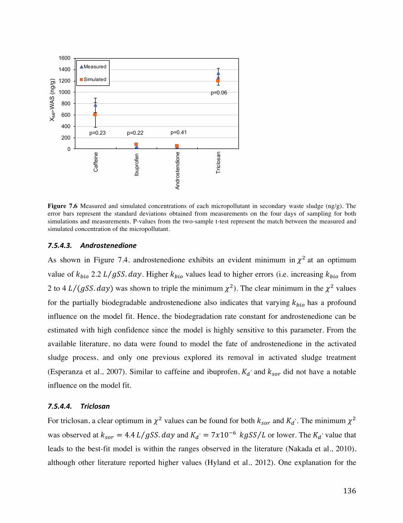
Figure 7.6 Measured and simulated concentrations of each micropollutant in secondary waste sludge (ng/g). The error bars represent the standard deviations obtained from measurements on the four days of sampling for both simulations and measurements. P-values from the two-sample t-test represent the match between the measured and simulated concentration of the micropollutant.

As shown in Figure 7.4, androstenedione exhibits an evident minimum in at an optimum

value of 2.2 . Higher values lead to higher errors (i.e. increasing from

2 to 4 was shown to triple the minimum ). The clear minimum in the values

for the partially biodegradable androstenedione also indicates that varying has a profound

influence on the model fit. Hence, the biodegradation rate constant for androstenedione can be

estimated with high confidence since the model is highly sensitive to this parameter. From the

available literature, no data were found to model the fate of androstenedione in the activated

sludge process, and only one previous explored its removal in activated sludge treatment

(Esperanza et al., 2007). Similar to caffeine and ibuprofen, and did not have a notable

influence on the model fit.

For triclosan, a clear optimum in values can be found for both and . The minimum

was observed at and or lower. The value that

leads to the best-fit model is within the ranges observed in the literature (Nakada et al., 2010),

although other literature reported higher values (Hyland et al., 2012). One explanation for the

observed being at the lower end of the literature values is the addition of ferric chloride in the

unit under study, which alters the properties of the sludge, potentially increasing the sorption

potential of MPs onto it. In fact, it was previously observed that chemical additions to activated

sludge decreases the value of for triclosan (Zhu, 2014). Using the optimum and

resulted in predicted particulate underflow concentrations that correspond to the measurements

with p-value >0.05, and the concentration in the secondary effluent also showed a fairly good

match with measurements (Figure 7.6 and Figure 7.5, respectively). Unlike sorption parameters,

wide variations in the value did not lead to changes in the model fit, indicating low

sensitivity of the model to this parameter.

7.5.5. Dynamic local sensitivity analysis After obtaining the optimal values of the most effective parameters for each of the four

micropollutants, a local sensitivity analysis was performed to investigate the dynamic sensitivity

of the different model variables throughout the four-day simulations, as shown in Figure 7.7.

This analysis provides information to link the model’s sensitivity to parameters with the

dynamics of input MP concentration and process conditions. Such analysis can provide valuable

information for the design of future measurement campaigns based on expected influent dynamic

conditions. For illustration, this analysis was performed for caffeine and triclosan only, since

their behaviour in activated sludge treatment was shown to be influenced by different fate

processes and their concentration in the influent is highly dynamic. Using WEST’s default

perturbation factor (i.e. the factor change in the parameter) of 10-6, inconclusive sensitivity

profiles were obtained, due to interference of numerical errors with the small effects on output

variable caused by the applied perturbations, due to the very low MP concentrations (De Pauw &

Vanrolleghem, 2006). Hence, the perturbation factor was set to a higher value of 10-2, and the

assumption of linearity of the sensitivity was verified to be still valid by the equality of the

backward and forward relative sensitivities (i.e. by both increasing and decreasing the parameter

with the same perturbation) (De Pauw & Vanrolleghem, 2006).

As shown in Figure 7.7, for caffeine at the best-fit parameters, the most influential parameter on

the soluble micropollutant concentrations is , which is in agreement with the observations

made in the previous section. This is supported by numerical sensitivity values indicating that a

100% theoretical change in the parameter results in >100% change in soluble micropollutant

concentrations at all monitored locations. On the contrary, the sensitivity to was low (<50%

change in XMP and SMP / 100% change in parameter), while the sensitivity to that describes

sorption equilibrium was high for the micropollutant concentration in the waste sludge only. A

notable reduction in the sensitivity of SMP to is observed to take place on the third day. The

specific time where the sensitivity to is lowest corresponds to a drastic increase in the

concentration of caffeine at the input to the activated sludge unit (i.e. from, 5,920 ng/L to 40,700

ng/L) and also at the headworks (i.e. from 4,813 ng/L to 50,800 ng/L). The effect of the increase

in input concentration on the sensitivity of SMP to is mathematically reasonable, since the

expression of the time-dependent SMP obtained from the numerical solution of Eq. 7.3 contains all

the following: the parameter , the incoming MP concentration and the initial MP

concentration (affected by previous incoming concentrations). A lower sensitivity to , as

observed on the third day, indicates that parameter value is not significantly affecting the

simulation due to other influences on the system. This is expected to increase the uncertainty of

the calibrated value if data were only available in such circumstances. Hence, avoiding

sampling during expected sharp dynamics in input caffeine (i.e. such as over weekdays and

weekends or around peak periods during the day for high-frequency samples) improves the

calibration of by eliminating data in low sensitivity conditions.

For triclosan, hypothetically increasing by 100% increased the soluble MP concentration by

10-40% and decreased the particulate concentration (in ng/L) by <5%, which is reasonably

explained by the higher calculated associated with the larger value of input . Increasing

by 100% was continuously shown to decrease the soluble MP concentration by 40-100% at

all locations of the activated sludge. Considering that in the input, the soluble to particulate MP

fraction (i.e. average of 3x10-4 ) is higher than that for secondary sludge at equilibrium

determined by (1x10-5 ), faster kinetics towards equilibrium will continuously reduce

the soluble MP concentration to achieve . The amount of reduction in the soluble MP

concentration due to perturbations in exhibited a time-dependent profile with higher

reductions in SMP (i.e. higher sensitivity to ) observed on the first and the third days where

the soluble load is the highest. This further emphasizes the impact of the input MP concentration

profile on the model’s sensitivity. The sensitivity of the particulate MP concentration to all

model parameters was lower than that of the soluble MP concentration (i.e. <20% change in XMP

for 100% theoretical change in parameter). This indicates that in the case of triclosan, measuring

the micropollutant concentration in the aqueous phase might be sufficient for calibration, due to

the higher sensitivity of the aqueous phase to the model parameters compared to the particulate

phase

Figure 7.7 Dynamic local sensitivity of the MP soluble concentrations (upper graphs) and particulate concentrations (lower graphs) in different locations: AE, SE and WAS to small perturbations in the three parameters for caffeine (a & b) and triclosan (c & d).

7.6. Conclusion

In this study, a model calibrated for conventional pollutants was extended to include MP fate

processes and was subsequently calibrated for a number of specific MPs of different classes

using full-scale measurements. The micropollutants’ fate processes were included in the

bioreactor model through an available extension of the ASM2d model and in the secondary

clarifier model by extending the Bürger-Diehl settler model for the first time to include the

propagation and the fate processes of MPs. Comparing results from the reactive and non-reactive

settler models indicated that a mismatch of 100% in the simulated micropollutant soluble

concentration at the underflow of the settler would occur as a result of ignoring biodegradation

taking place in the settler for the case of the highly biodegradable caffeine. A Monte Carlo based

scenario analysis was used to find optimal parameter values, as well as to provide information on

parameter’s identifiability and the model’s global sensitivity. Depending on the process that

plays the major role in the fate of a specific micropollutant, different model parameters could

affect the fit of the model to different extents, which eventually determines the identifiability of

the calibrated parameters. While for the highly biodegradable caffeine and ibuprofen, was

found to be the most significant parameter influencing the fit of the model, for triclosan, both

sorption parameters and were more significant. For androstenedione, which is mildly

degradable, the showed a clearer optimum compared to caffeine and ibuprofen. Dynamic

local sensitivity analysis was performed and proposed to serve as a tool in the design of sampling

campaigns for improved calibration of model parameters, since it provides insights on preferable

input dynamics during sampling, as well as on necessary types of measurements (i.e. particulate

or soluble MP concentration). These analyses provided novel insights on the sensitivity of a

micropollutant activated sludge model to the different model parameters, as well as on the

temporal variability in the sensitivity in relation to input dynamics. The sampling campaign used,

limited in resource and time requirements, indicated a potential for future applications of this fate

model by WWTP operators for the purpose of developing risk assessment tools to evaluate the

discharge of micropollutants into the environment.

7.7. Acknowledgements

The authors acknowledge the staff at the Guelph WWTPs for their support during the sampling

campaign. The authors thank Prof. Chris Metcalfe and Dr. Tamanna Sultana for the chemical

analysis of the target compounds. We gratefully acknowledge the McGill Engineering doctoral

award for supporting Zeina Baalbaki. Funding for this study was provided by a research grant to

Viviane Yargeau (PI) and colleagues (Chris Metcalfe and Peter Vanrolleghem) from the Natural

Sciences and Engineering Research Council (NSERC) of Canada through the Strategic Grants

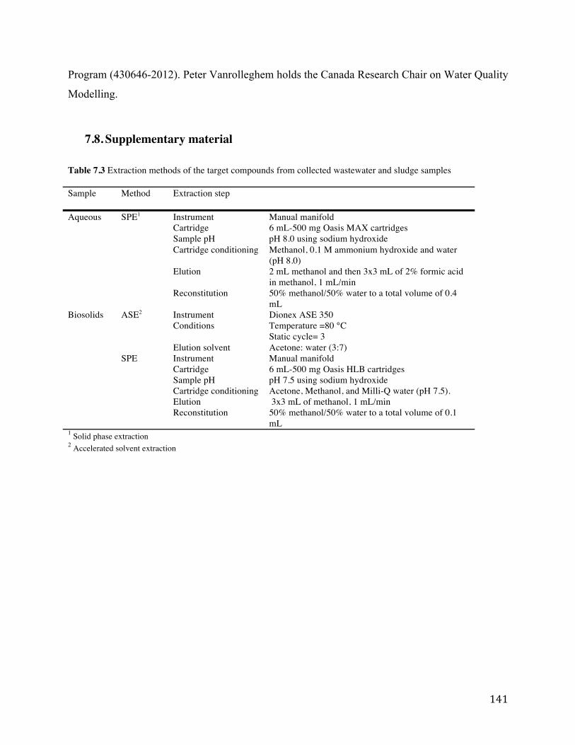
Program (430646-2012). Peter Vanrolleghem holds the Canada Research Chair on Water Quality

Modelling.

7.8. Supplementary material

Table 7.3 Extraction methods of the target compounds from collected wastewater and sludge samples

Sample Method Extraction step

Aqueous

SPE1 Instrument Manual manifold Cartridge 6 mL-500 mg Oasis MAX cartridges Sample pH pH 8.0 using sodium hydroxide Cartridge conditioning Methanol, 0.1 M ammonium hydroxide and water

(pH 8.0) Elution 2 mL methanol and then 3x3 mL of 2% formic acid

in methanol, 1 mL/min Reconstitution 50% methanol/50% water to a total volume of 0.4

mL Biosolids

ASE2 Instrument Dionex ASE 350 Conditions Temperature =80 °C

Static cycle= 3 Elution solvent Acetone: water (3:7)

SPE Instrument Manual manifold Cartridge 6 mL-500 mg Oasis HLB cartridges Sample pH pH 7.5 using sodium hydroxide Cartridge conditioning Acetone, Methanol, and Milli-Q water (pH 7.5). Elution 3x3 mL of methanol, 1 mL/min Reconstitution 50% methanol/50% water to a total volume of 0.1

mL 1 Solid phase extraction 2 Accelerated solvent extraction

8. ORIGINAL COUNTRIBUTIONS The original contributions of this PhD project are:

I. The demonstration of the ability of the “fractionated approach” to account for differences between treatment plants and the implementation of the method for the first time as an improved sampling and removal calculation strategy for the investigation of CEC removal in primary and tertiary treatment steps. Although the fractionated

approach was previously applied twice for CEC removal calculation, the application was

limited for a number of CECs and within the process of activated sludge treatment only, but

no data reported removal in primary and tertiary treatment steps determined using this

approach. The removal of some target CECs was examined for the first time in rotating

biological contactors and sand filters. In addition to that, the fractionated approach was used

in the present study to compare the effect of hydraulic differences on the CEC removal

calculations between two full-scale WWTPs and between various treatment units within a

WWTP.

II. Coupling mass balance analysis of CECs in a full-scale WWTP with the fractionated approach providing improved data of fate of CECs and for the first time data were provided on the fate of some CECs (few drugs of abuse and androstenedione) in primary sludge and activated sludge. Furthermore, a biosolids extraction method

previously suggested for beta-blockers was proven to yield satisfactory recoveries for the

studied drugs of abuse.

III. Calibration of an ASM2d-based CEC fate model for several CECs of different classes

after coupling to a reactive settler. The reactive settler model was developed in this project

as an extension of the Bürger-Diehl model, and in addition to fate processes, it was also

extended to account for the propagation of soluble and particulate CECs in the settler due to

both flow and gravity settling. Calibrated parameter values were reported for the first time

for some CECs. Prior calibration of solids in the activated sludge provided novel insights on

the impact of the chemically-enhanced primary treatment on the solids balance that is

expected to impact the fate of CECs.

IV. Exploration of the sensitivity of the fit and output of the fate model to the model parameters for CECs with different fate characteristics. To date, no published studies had

performed analysis of the global and local sensitivity of micropollutant activated sludge

models to the model parameters.

9. CONCLUSIONS The thesis examined the removal of 26 target contaminants of emerging concern in different

steps of wastewater treatment plants. One novelty of the work performed is the consideration of

the hydrodynamics of the treatment units for the CEC removal calculations by comparing the

hydraulic characteristics of two WWTPs and the resulting removal calculations. Another major

contribution is the use of a mass balance of the CEC load performed by measuring the CEC load

sorbed to solids in primary and secondary treatment steps, which allowed the quantification of

the contribution of different fate pathways for each target CEC. Lastly, a model was developed

and calibrated to predict the fate of four target CECs in the activated sludge process accounting

for fate processes in the secondary clarifier for the first time.

The results showed that:

I. Activated sludge processes with different configurations showed different hydraulic

characteristics and, hence, the calculation of removal of CECs by these units had to be

adjusted accordingly. Obtaining reliable removal data using the fractionated approach

involves determining the proper load fractions representing the output CEC load in terms of

incoming loads of previous days, which were shown to be different for different activated

sludge units, depending on the hydraulic retention time and the extent of mixing of each unit.

II. The best-fit hydraulic models obtained for the primary and tertiary wastewater treatment

units suggested a low extent of mixing compared to the secondary treatment step. Hence, for

these units, most of the CEC load discharged on a specific day corresponded to the load

entering on the same day with lower fractions coming from previous days compared to the

activated sludge process.

III. A mass balance analysis demonstrated that in the activated sludge unit, biodegradation was

the major removal process for most of the investigated CECs, while sorption did not play a

significant role in the removal of most target CECs (i.e. <5%), except for estrone, triclosan

and trimethoprim (i.e. 29-47%). The mass balance analysis in the primary clarifier indicated

poor removal for most of the target CECs, with degradation contributing to the removal of

some CECs, such as ibuprofen, androstenedione, sulfamethoxazole and triclosan.

IV. The studied tertiary treatment steps, rotating biological contactors and sand filtration, were

generally less efficient at removing target CECs than secondary treatment by activated

sludge, although these tertiary steps were found to play a role in the removal of conventional

pollutants such as ammonia and solids.

V. Measuring the concentrations of the major metabolites of carbamazepine indicated potential

inter-transformation between the metabolites and the parent compounds during wastewater

treatment. This provided an explanation for the persistence or negative elimination of

carbamazepine, which were frequently reported in the literature and theoretically linked to

the hydraulics effect on the removal calculations and potential deconjugation of metabolites.

Since the hydraulics were properly accounted for in the current study, the observations must

be linked to the transformations discussed above.

VI. The solids modelling performed for the studied activated sludge unit, as a prerequisite to

modelling the fate of CECs, indicated that the particulate to soluble organics ratio in the

effluent of CEPT obtained from characterization (i.e. representation in terms of model

components) differed from the ratio observed for effluents from conventional primary

clarifiers. Results also showed that special considerations were required to characterize the

solids in the primary effluent, which was linked to the effect of CEPT on the composition of

the primary effluent.

VII. From the CEC fate model describing the CEC removal by activated sludge treatment, it was

observed that a model that ignores the biodegradation in the secondary clarifier, which is

general practice, potentially overestimates the settler’s underflow concentration of caffeine

that is known to be highly biodegradable. Hence, this study showed that to model the fate of

CECs in activated sludge units, it is essential to account for the fate processes not only in the

aeration tanks but also in the secondary clarifier. The state-of-the-art Bürger-Diehl model for

secondary clarifiers was thus extended for the first time with CEC fate submodels.

VIII. The fit of the secondary treatment fate model was shown to be sensitive to different

parameters depending on the compound of interest (i.e. was more significant for the

prediction of androstenedione followed by ibuprofen and caffeine, while and were

more important to predict the fate of triclosan). The most influential parameter set was

observed to depend on the target CEC and its corresponding predominant fate process (i.e.

biodegradation or sorption), and indicated the need to identify specific parameters to focus on

during calibration.

IX. From the dynamic sensitivity analysis, it was shown that the profile of the incoming CEC

concentration measured during sampling campaign and used in the model input can

potentially cause temporal variability in the model’s sensitivity to the parameters.

Considering that calibrating a model parameter based on instants of low sensitivity to the

parameter reduces the confidence in the obtained calibrated parameter, it is important to

enhance the sensitivity of the model or to measure at those instances where sensitivity is

high. Hence, it is preferable to perform sampling campaigns at specific conditions of CEC

levels in the influent. For caffeine, the absence of sharp changes in the input concentrations

was found to enhance the model’s sensitivity to , while for triclosan a higher soluble to

particulate CEC concentration increased the sensitivity to .

10. RECOMMENDATIONS Based on the literature, results and conclusions of this study, the following areas were identified

to be in need for further consideration:

i. All the sampling campaigns in the present study were carried out to collect 24-h

composite samples on weekdays. Due to the previously proven variations in wastewater

composition throughout the week, it is recommended that future sampling campaigns

include both weekdays and weekends and more frequent sampling to account for diurnal

variations of CEC load. This would help to capture higher temporal variability of the

input CEC load and examine its effect on the removals and calibrated model parameters.

ii. Collection of higher volumes of aqueous samples enables the measurement of CEC

concentration in the suspended solids at each sampling location, including the settled

wastewater at the secondary effluent. This would further enhance the reliability of the

mass balance results and provide more data for a more detailed calibration of the CEC

fate model.

iii. In this project, the concentration of the main metabolites of carbamazepine were

measured and inter-transformations between these and their parent compound was

suggested. Being able to integrate these transformations into the CEC fate model in

activated sludge would improve the study of the fate of persistent CECs but is currently

beyond the capabilities of the existing models. Hence, further modifications of the CEC

fate model are recommended to introduce extra CEC components to the model base, as

well as simplified equations for their inter-transformations. iv. In the present study, the CEC fate model was calibrated using data from a full-scale

WWTP. Testing the model with data from other WWTPs would provide further

validation of the CEC fate models and the calibrated parameters. Sensitivity analysis of

the CEC fate model with respect to the conventional pollutants would also provide

insights on the effect of varying characteristics (i.e. solids concentrations and removals)

between the different WWTPs.

11. REFERENCES

APPENDIX I: SOLIDS SETTLING MODELS

Table A.1 Main differences between the Takács and the Bürger-Diehl settling models (Bürger et al., 2012; Bürger et al., 2011; Takács et al., 1991; Torfs et al., 2015).

Aspect Takács Bürger-Diehl Model 1-D (i.e. only vertical flow) 1-D (i.e. only vertical flow) Number of layers 10 layers The number of layers can be set by the user, with higher

number resulting in a physically-correct representation Boundary layers No boundary layers; i.e. the

concentration in the underflow of the clarifier is assumed equal to the concentration in the bottom layer

Two extra layers at the top and at the bottom to better describe the outlet concentration taking into account the effect of the outlet pipe

Settling Accounts for gravity settling Accounts for gravity settling and compression settling that is a phenomenon observed in high-concentration sludge present in the sludge blanket

Inlet dispersion The incoming solids are assumed to be distributed instantaneously and homogeneously over the feed layer

Accounts for dispersion by taking into account the mixing phenomenon in the feed layer as a function of the input flow rate