26-28 June 2015

Paper: ASAT-16-142-PP

16th International Conference on AEROSPACE SCIENCES & AVIATION TECHNOLOGY, ASAT - 16 – May 26 - 28, 2015, E-Mail: [email protected] Military Technical College, Kobry Elkobbah, Cairo, Egypt Tel : +(202) 24025292 – 24036138, Fax: +(202) 22621908

Smooth Curvature of Airfoils Meanline for a General

Turbomachinery Geometry Generator

Ahmed F. Nemnem ∗

and Mark G. Turner †

26-28 June 2015

Abstract:

The blade geometry design process is integral to the development and advancement of

compressors and turbines in gas turbines or aeroengines. An airfoil section design feature has

been added to a previously developed open source parametric 3D blade design tool. The

second derivative of the mean-line (related to the curvature) is controlled using B-splines to

create the airfoils. This is analytically integrated twice to obtain the mean-line. A smooth

thickness distribution is then added to the airfoil with two options either the Wennerstrom

distribution or a quartic B-spline thickness distribution. B-splines have also been

implemented to achieve customized airfoil leading and trailing edges. Geometry for a turbine,

compressor, and transonic fan are presented along with a demonstration of the importance of

airfoil smoothness.

Keywords: Meanline, Curvature, Geometry, Turbomachinery

Nomenclature

Greek Symbols

β*in The blade section inlet (leading edge) metal angle

β*out The blade section outlet (trailing edge) metal angle

χin Camber angle at section inlet (leading edge)

χout Camber angle at section exit (trailing edge)

ρ Density

ξ Stagger angle

* Aircraft and Aerospace Department, Military Technical College, Cairo, Egypt /email:

[email protected]

† School of Aerospace Systems, University of Cincinnati, Cincinnati, Ohio /email: [email protected]


Mathematical Symbols

(u− v) Non-dimentional spacing coordinate system for 2D section creation

ang Angle, arc tangent of the slope

Br The b-spline basis functions

C Curvature of a streamline

chrd The blade section nondimentional chord

ee Leading edge elongation parameter

k Scale factor to adjust for leading edge slope value

lecurv Leading edge curvature

lethk Leading edge thickness

mxthk The blade section max thickness ratio (t/c)

n Distance perpendicular to the streamline

ns B-spline order

nside Number of coordinate points in top and bottom airfoil curves

p Pressure

Pi+r General notation for spline control points

R Radius of curvature of the streamline

s Arc length in the (u− v) space

Si The b-spline parametric coordinate

sext Trailing edge (exit) slope tan(χout)

sinl Leading edge (inlet) slope tan(χin)

ss Leading edge Droop parameter

t Parameter used in b-spline calculation

tecurv Trailing edge curvature

tethk Trailing edge thickness

thk Section spline thickness distribution

thkmultip Thickness modifier B-spline at u position

thkmultipi(tu) Parametric thickness modifier B-spline

umxthk u location of the maximum thickness

2


V Velocity along a streamline

v(u) Camber at u position

x Distance along a streamline

Superscripts

′ First derivative

′′ Second derivative

′′′ Third derivative

Subscripts

bbot Airfoil bottom curve in (u− v) plane

btop Airfoil top curve in (u− v) plane

cp Control points array

le Leading edge point

u Parameter at u position

Abbreviations

3DBGB 3 Dimensional Blade Geometry Builder

ARL, AFRL Air Force Research Laboratories

LE Leading Edge

NACA National Advisory Committee for Aeronautics

NURBS Non-Uniform Rational B-Spline

INTRODUCTIONBlade design is a critical design stage through the full engine design process. In the earlydays, standard profile families were developed (i.e. NACA) in order to describe the profilewith a small number of parameters and be able to compare designs and test results ofdifferent aerodynamic shapes. Later, when physical effects of boundary layer separations,turbulence, skin friction, shape factors and non-steady loss generating mechanisms wereinvestigated, a new style of optimized blade airfoils were designed. One of them is theparametric airfoils that improves the engineering design process and allows fast creation,optimization and manufacture of the blades.

There were different approaches used to design some new airfoils rather than the tra-ditional ones. J. Burman et al. [[1], [2]] defined the suction and pressure sides with athickness distribution and camber line splines. The leading and trailing edges end nodesare shared with airfoil surface such that the intersection points between them have slopecontinuity. BMW Rolls-Royce created “A parametric blade design system” by Jugen M.

3


Anders et al. [3] that described the 2D airfoil as two independent patches of higher orderBezier curves plus leading edge (circular and elliptic) and trailing edge with slope conti-nuity at the contact points. The previous two approaches insures a slope continuity in theconnection points which will have discontinuities in the higher derivatives. This can leadto a kink in mach number and pressure distribution over the leading edge. Koini et al. [4]describes each cross section as a mean-line second order NURBS and a distribution ofpoints imposed on it which forms the control points for the blade section NURBS. Thisapproach gives a smooth blade surface but when trying to apply control, for example onthe section leading edge, this will not be trivial as there are not enough parameters tomake local changes to the blade sections.

Korakianitis et al. [5] generated the 2D blade shape by defining the geometry nearthe trailing edge with two third-order polynomials and the main portion of the blade de-scribed by a surface curvature distribution spline, while the leading edge was definedwith a parabolic construction line with two thickness distributions. Korakianitis definesthe curvature distribution of the blade surfaces as a spline, then matches the slope ofthe blade surfaces curvature spline with that of the four contact points with the leadingand trailing edges. Just defining the upper and lower surfaces make it possible to have anegative thickness distribution. Negative thickness distribution or even a very thin bladewithout a specified smooth thickness distribution are either not realistic or will not meetstructural requirements. Korakianitis approach is considered the most relevant one tothe presented technique. Considering the curvature equation, the pressure distributionis directly affected by the curvature, as will be explained below, with smooth thicknessdistribution defined.

The open source General Turbomachinery Geometry Generator was created by Sid-dappaji et al. [[6], [7]] to generate 3D blades for various kinds of turbomachinery. Newfeatures are added to the Geometry Generator that improves the 2D airfoil design pro-cess. The motivation to use the curvature-defined mean-line approach together with themethodology is explained below.

The 3DBGB blade generator is a free license blade builder. It can be downloadedfrom ( http://gtsl.ase.uc.edu/3DBGB/).

MOTIVATIONThe curvature has a major effect on the blade performance. It affects directly the pressuredistribution (loading distribution) over the blade surface. This is a basic fluid concept asexplained by Fox et al. [8] when describing the motion of a particle in a steady flow.

In the stream wise direction, Bernoulli equation can be derived. When applied in thenormal n direction, the equation normal to the streamline becomes,

1ρ

∂ p∂n

=V 2

R=CV 2 (1)

where, R is the radius of curvature of the streamline, C is the curvature of the stream-line, n is the distance perpendicular to the streamlines and V is the velocity along astreamlines. Figure 1 shows radius of curvature, direction vectors along and normal tothe streamline.

This indicates “Pressure increases in the direction outward from the center of curva-ture of the streamline” [8]. This shows that the streamline curvature ( 1

R ) has a direct effect

4


Figure 1: Radius of curvature normal to the streamlines.

on the pressure gradient in direction normal to the streamline which in other words af-fect directly the “Blade loading distribution”. This conclusion was mentioned in 1973 byKeith et al. showing again the solution for the pressure distribution over a nacelle surfaceis related to the curvature distribution [9].

As a result, starting with curvature to define the airfoil geometry is a direct repre-sentation of the loading over the blade surface. Specifying the camber-line through thecurvature, allows going to higher order of smoothness with a smaller order of designvariables rather than defining the camber-line with points. Adding a high order positivethickness distribution to the curvature-defined mean-line avoids any thickness negativedistribution along the blade.

Geometry & Coordinate systems

Coordinate systems:Creating the 3D blade is accomplished through several steps, each have a separate coor-dinate system [6]. Explanation of the coordinates systems are as follows:

The Meridional (xs− rs) coordinate system:

The Meridional 2D (axial-radial) coordinate system that describes the axisymmetric stream-line coordinates as shown in Figure 2,

Figure 2: Meridional view of the blade showing the axisymmetric streamlines [6].

5


The (u− v) coordinate system:

The camber-line is created in the (u− v) space. Then the thickness distribution, leadingand trailing edge are added to the camber-line to create the 2D blade section as shownin Figure 3. Lean and sweep are defined either tangent and normal to the blade (Denton[10]), or in the meridional and tangential (m′,θ) directions (Smith and Yeh [11]). Thelean and sweep tangent to the blade is applied in the (u− v) coordinates after the sectionis created. The stacking offset relative to percent chord is also applied in the (u− v)coordinate system.

Figure 3: (u− v) coordinate system [6].

The (m′,θ) coordinate system:

The blade sections are created in the (u− v) space, then rotated by stagger angle (ξ ) andscaled either by the non-dimensional calculated chord (chrd) or user defined chord axialprojection (chrdx), as shown in Figure 4. The lean and sweep are applied in the (m′,θ)coordinate system.

Figure 4: Relation between (m′−θ) and (u− v)coordinate systems [6].

The (r− x−θ) coordinate system:

This a 3D cylindrical coordinate system at which the 2D sections in the (m′,θ) spaceare mapped on the streamline coordinates that in turn make the sections in 3D space asdescribed by Siddappaji [6].

6


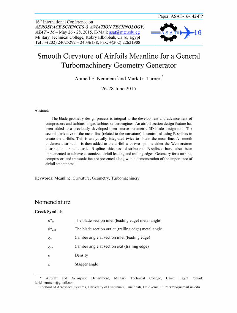
Figure 5: (r− x−θ) 3D coordinate system [6].

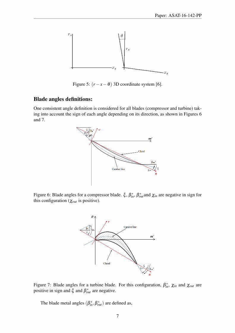
Blade angles definitions:One consistent angle definition is considered for all blades (compressor and turbine) tak-ing into account the sign of each angle depending on its direction, as shown in Figures 6and 7.

Figure 6: Blade angles for a compressor blade. ξ , β ∗in, β ∗outand χin are negative in sign forthis configuration (χout is positive).

Figure 7: Blade angles for a turbine blade. For this configuration, β ∗in, χin and χout arepositive in sign and ξ and β ∗out are negative.

The blade metal angles (β ∗in,β∗out) are defined as,

7


β∗in =χin +ξ (2)

β∗out =χout +ξ (3)

By a simple manipulation of these equations, the stagger angle can be written as,

ξ =

(β ∗in +β ∗out

2

)−(

χin +χout

2

)(4)

METHODOLOGY

2D airfoils to construct 3D blade:The 3D blade is generated by stacking the 2D sections created in (m′,θ) space. Figure 8shows the flow chart to the curvature-defined 2D section design process. The data inputfile describes the streamlines in the (xs− rs) space and blade parameters such as sec-tion metal angles (βin,βout), chord (chrd) and maximum thickness (mxthk). The controlparameters describe the sections curvature, thickness modifier, leading and trailing edgeshapes.

Figure 8: 2D Section design flow chart.

Cubic and Quartic B-splines:A parametric Cubic[12] and Quartic [[13], [14]] B-spline are used to create the mean-line,thickness distribution and thickness modifier of the 2D sections.

The general B-spline parametric function is given as,

Si(t) =ns

∑r=0

Pi+rBr(t) f or [0≤ t ≤ 1] (5)

where, Pi,Pi+1,Pi+2,Pi+3,Pi+4... are the control points influencing the B-spline, asshown in figure 9 and ns is the B-spline order.

8


Figure 9: Cubic B-spline[12].

For a Cubic B-spline, ns = 3, where “t” is a parameter used for each segment calcula-tion and Bi(t) are the basis functions for the spline calculation as shown below,

B0(t) =−t3 +3t2-3t +1

6=

(1− t)3

6

B1(t) =3t3−6t2 +4

6

B2(t) =−3t3 +3t2 +3t +1

6

B3(t) =t3

6(6)

For the Quartic B-spline, ns = 4. The quartic basis functions are,

B1(t) =(1− t)4

24

B2(t) =

(−4t4 +12t3−6t2−12t +11

)24

B3(t) =

(6t4−12t3−6t2 +12t +11

)24

B4(t) =

(−4t4 +4t3 +6t2 +4t +1

)24

B5(t) =t4

24(7)

Quartic B-spline basis functions and their derivatives are shown in Table 1.

Table 1: Quartic B-spline derivatives coefficients.

9


Mean-line calculations:Korakianitis [5] and Sherar [15] describe the curvature as a function of the first and secondderivatives,

C =1R=

y′′

[1+ y′2](3/2)(8)

where, y′′ = d2ydx2 referring to the reference coordinate system.

The second derivative of the mean-line is defined as a cubic B-spline using equation(5) at ns = 3,

v′′(u) =Si(tu) =3

∑r=0

Pi+rBr(tu) (9)

where, tu is the parameter t at the coordinate position u .Figure 10 shows the second derivative B-spline that indicates the curvature of the

whole blade section from leading edge to trailing edge (from u = 0 to u = 1).

Figure 10: Second derivative B-spline with control points.

The second derivative of the camber line is the derivative of the slope (v′(u)). Usinganalytical integration of the cubic B-spline, the slope is calculated, and plotted as shownin figure 11,

v′(u) =ˆ

k(v′′(u)

)du+ tan(χin) (10)

where, k is a scale factor evaluated to enforce the trailing edge angle. The inclusion ofthe scale factor means the magnitude of the second derivative input is adjusted to ensurethe blade has the overall specified camber (angle differences).

The slopes sinl,sext are related by

10


v′ (0) = sinl = tan(χin) (11)v′ (1) = sext = tan(χout) (12)

Figure 11: First derivative (Slope) B-spline.

The camber-line is obtained through an iterative process by integrating the slope curveas follows,

v(u) =ˆ

v′(u)du (13)

v(0) =0 (14)v(1) =0 (15)

Equation (14) has been used to evaluate the constant of integration in equation (13).There are 4 coupled equations (2), (3), (12) and (15) with 4 unknowns (k,ξ ,χin,χout). Theslope and camber equations (10) and (13) are initially evaluated with an initial estimationof the stagger angle (ξ ) (equation (4)) assuming initially the sum of blade angles is zero,(χin +χout) = 0.

A secant method is used to solve equations (10) and (13) enforcing the boundary con-dition stated in equation (15). Once equation (15) is satisfied, stagger angle is recalculatedusing equation (4). Manipulating equations (2) and (3), blade angles are evaluated usingequations (16) and (17).The camber line can then be plotted as shown in figure 12.

χin =β∗in−ξ (16)

χout =β∗out−ξ (17)

The curvature along the mean-line can be defined as

C =∂ χ

∂ s(18)

11


where, s is the arc length in the (u− v) space. The second derivatives v′′ are integratedinstead of the curvature to eliminate the non linearity of the arc length. From equation(8), the second derivative has the characteristic of the curvature.

Figure 12: Camber line B-spline.

Airfoil thickness distributions:There are two options for thickness distribution: the Wennerstrom thickness distribution(third order polynomial), as explained in the book by Wennerstrom [16] and a Quartic B-spline thickness distribution. The control points for the later are calculated from solvinga system of equations that describe all the constrains on the blade section. Leading andtrailing edge thicknesses together with the location and value of the maximum thicknesson the blade section are all constraints used to calculate the thickness spline control points.The system has a total of 18 control points for each blade section. The total thicknessdistribution (thk) is calculated by simple subtraction between the upper and lower sidesthicknesses. This results in a blade surface with a 4th order spline smoothness. The airfoiltop curve quartic B-spline is considered in figure 13 with the location of the maximum,leading and trailing edges thicknesses.

Spline quartic Thickness Modifier:For increased thickness control, a thickness modifier spline (thkmultip(u)) is added tothe original thickness distribution,

thkmultip(u) = thkmultipi(tu) =4

∑r=0

Pi+rBr(tu) f or [0≤ t ≤ 1] (19)

The thickness modifier values are added to the different options of thickness distribu-tion such that the total thickness is increased as follows,

thk = thk ∗ (thkmultip+1) (20)

12


Figure 13: Airfoil top curve quartic thickness B-spline.

The thickness modifier control points are specified in the control parameters input toobtain the best loading distribution over the blade section surface. The quartic thicknessmodifier B-spline is shown in figure 14.

Figure 14: Spline thickness modifier.

2D airfoil creation:The top and bottom airfoil curves are then calculated using the camber line, thicknessdistribution and blade angles at each coordinate point as follows,

ubtop = u −thk ∗ sin(ang)vbtop = v +thk ∗ cos(ang)ubbot = u +thk ∗ sin(ang)vbbot = v −thk ∗ cos(ang) (21)

13


where,(ubtop,vbtop

),(ubbot ,vbbot) are nside coordinates of the airfoil top and bottom

curves in(u− v) plane, respectively. Each has a number of points (nside). thk is half theactual blade thickness added to it the thickness modifier (thkmultip) value at each point.

ang is the angle at each coordinate u defined by,

ang = tan−1(v′) (22)

The airfoil top and bottom curve coordinates are then put in one array (ub,vb) . Itstarts from the trailing edge, rotating counter clockwise through leading edge and returnsback to the trailing edge point with total (2nside−1) number of points. The airfoil is stillin the (u− v) plane.

Leading edge option:The leading edge is an essential feature that affects the flow over the blade surface. Threeleading edge options are available with the geometry generator. The default leading edgeoption is an elliptical leading edge mounted when using the Wennerstrom thickness dis-tribution, as explained by Siddappaji et al. [[7], [6]].

The second option is implicitly defined in the quartic B-spline thickness distribution.The second leading edge shape depends on the LE constraints defined when calculat-ing the spline thickness distribution. (lethk, lecurv) are the LE parameters defined whensolving for the spline thickness distribution control points for the entire blade section.

The third option is a quartic leading edge B-spline. This type of leading edge is in-stalled on the blade in the (u− v) plane after full creation of the blade section. Whenchoosing this option, the current installed leading edge is removed and a quartic B-splineleading edge is connected instead. The B-spline is connected with the blade section con-tact points by matching the first, second and third derivatives. The following equationsdescribe the relation between the derivatives w.r.t. u and the spline parametric derivativesw.r.t. t.

dvdu

=

(dvdt

)(dtdx

)=

v′(t)u′(t)

d2vdu2 =

(d2vdt2

)(dt2

d2x

)=

v′′(t)u′′(t)

d3vdu3 =

(d3vdt3

)(dt3

d3x

)=

v′′′(t)u′′′(t)

(23)

Matching the first three derivatives gives smooth and continuous curvature and slopeof the curvature at the contact points. The derivatives are calculated using higher orderfinite difference with a very small step size to then set equal to the B-spline derivatives att = 0.

Table 1 shows the quartic B-spline basis functions and its derivatives that are used inmatching process. The control parameters serve to adjust a good matching between theleading edge and the blade section surface, besides controlling the leading edge shapeas well. The leading edge B-spline is controlled by 9 parameters, these parameters arethe leading edge thickness (lethk), droop (ss), elongation (ee) and 6 more control pointparameters. The droop and elongation are shown in the figure 15.

14


Figure 15: LE Droop and Elongation.

An algebraic system of equations are solved to calculate 9 control points describingthe quartic B-spline leading edge as plotted in figure 16. The Fourth and sixth controlpoints are determined with two parameters, levertex−ang, levertex−dis. The first parameter(levertex−ang) allows the identification of the leading edge vertex angle in degrees. Whilethe second variable (levertex−dis) specify a ratio for the distance between the eccentricitycontrol point and the upper (4th) and lower (6th) control points,

ucp(4)−ucp(5) = (levertex−dis) · cos(

levertex−ang

2

)ucp(5)−ucp(6) = (levertex−dis) · cos

(levertex−ang

2

)vcp(4)− vcp(5) = (levertex−dis) · sin

(levertex−ang

2

)vcp(5)− vcp(6) = −(levertex−dis) · sin

(levertex−ang

2

)(24)

A scheme for the leading edge control points and LE shape parameters is shown infigure 16.

15


Figure 16: LE B-spline with control points.

Trailing edge options:The options for the trailing edge are the same as the leading edge with the added optionsof a circular arc and a blunt trailing edge.

2D airfoil stacking, rotation and scaling:The final steps in the 2D blade section creation are the sections 2D stacking, rotation andscaling. The 2D stacking process is done in the (u− v) plane by translating each sectionto its stacking user defined position. Then rotation by the stagger angle (ξ ) and scalingwith the chord value (chrd) are both done to set the blade sections in the (m′,θ) plane,

chrd =chrdx/ |cosξ |m′bstgr =ubcos(ξ )+ vbsin(ξ )

θbstgr =−ubsin(ξ )+ vbcos(ξ )

m′=m

′bstgr(chrd)

θ =θbstgr(chrd) (25)

The (m′,θ) blade sections are then projected on the stream lines in the 3D (r,x,θ)plane. Coordinates are mapped to the Cartesian (x,y,z) coordinate system to give 3Dblade sections that is compatible with the CAD systems as explained by Siddappaji [7].

Demonstration of CapabilityThis 2D blade section generation technique improves the smoothness of the blade surfaceto the fourth order spline degree. That ensures the curvature and slope of curvature to becontinuous all over the blade surface. The loading distribution over the blade surface isimproved with no spikes in Mach number. This prevents local acceleration and deceler-ation of the flow. A demonstration for the new capability is discussed below. A turbine

16


Table 2: The turbine hub section data from NASA report [17].Rotor second stage hub section data

Number of blades 70Rotor inlet relative flow angle 31.5o

Rotor exit relative flow angle 59.9o

Rotor inlet relative Mach No. 0.339Rotor exit relative Mach No. 0.724

Hub radius 31.115 cmTrailing edge thickness 0.1575 cm

Axial width 3.353 cm

blade is created such that it is similar to the second stage turbine rotor created by Timko,L. P. [17]. The hub section is chosen for comparison. The 2D rotor hub section data isstated in Table 2. The blade section is also shown in figure 17. All prior figures in thispaper to describe the process (Figures 10-14 & 16) come from this demonstration case.

Figure 17: Test case turbine hub section [17].

The Test case input files are then created guided with data from Table 2. The Reynoldsnumber is taken

(1.76X105)as specified for rig design point in the reference report. The

output hub blade section is analyzed using MISES [18] such that the inlet and exit Machnumbers are matched. A Mach number distribution is plotted and used as a demonstrationexample for the 3DBGB capabilities. The resulting turbine hub section is shown in figure18.

17


Figure 18: Turbine blade hub section in (m′,θ) plane.

Smoothness Improvement and shape controlThe second derivative of a hub turbine blade section surface is calculated using finitedifference. It is plotted starting from the trailing edge through top surface, leading edge,bottom surface and back to trailing edge as shown in figure 19. It shows the secondderivative has a smooth transition from the top to the bottom surface. Figure 20 shows azoomed view of the leading edge region.

Figure 19: Second derivative over turbine blade surface.

Mach number distributionA fine grid viscous run using MISES [18] is performed for the turbine blade hub sectionto examine the blade surface smoothness. The grid and Mach number distribution areshown in figures 21. The Mach number is found to be smooth all over the blade surface

18


Figure 20: The Second derivative at the Leading edge.

as shown in figures 23 and 24. No spikes or local accelerations and decelerations arenoticed. Figure 22 can be compared with the loading from the EEE report in figure 17.

Figure 21: Turbine MISES Fine Grid.

19


Figure 22: Mach number distribution plot using fine grid MISES run.

Figure 23: Turbine passage Mach number contours.

Figure 24: Turbine leading edge Mach number contours.

20


Variety of Airfoil shapes using Curvature Technique3DBGB is capable of generating different airfoil shapes span-wise for a blade design.The curvature technique gives flexibility in controlling the airfoil shape. A compressorand transonic fan hub sections are created as additional examples. The second derivativespline associated with each case is plotted too. Figures 25 and 26 shows a similar designfor a transonic fan tip section that was designed by Drayton [19]. 3DBGB input files arecreated to match the original blade design considering the metal angles and the thicknessdistribution. Smith [20] was investigating the key area locations. He stated how the criti-cal flow area is affected with the changes of the relative total pressure along a streamline.This shows the importance of indicating the mouth and throat areas. The 2D throat, mouthand exit for the transonic fan are plotted in figure 27. The area ratio (AT

A1/

A∗TA∗1

) is calculatedfor the transonic fan and plotted on Smith curve [20], which gives a 4% throat margin forthis case as shown in figure 28.

Figure 25: Second derivative distribution for the transonic fan.

Figure 26: Transonic fan tip section.

Another example demonstrated is a hub section for EEE NASA - GE 3rd stage com-pressor rotor [21]. The second derivative distribution is created for the blade hub sectionas shown in figure 29. The blade 2D sections are constructed with input file that matchesthe section properties. Figure 30 shows the 2D hub section for the EEE 3rd rotor blade.

21


Figure 27: The 2D throat, mouth and exit positions for the transonic fan tip.

Figure 28: The throat area/capture area ratio method to calculate throat margin of thetransonic fan as described by [20]. The black circles are the 12 streamline from thereference. The red point is the case shown in figure 27.

Figure 29: Second derivative distribution for EEE 3rd stage rotor.

The 3D blade of the EEE 3rd stage rotor is then created using 21 sections as shown in

22


Figure 30: 3rd rotor hub section from EEE NASA report.

figure 31 using SOLIDWORKS [22] (CAD program).

Figure 31: The 3DBGB blade for the EEE 3rd stage rotor.

Another compressor test case has been set up to to clarify the use of the curvaturetechnique. The 8th rotor for the GE EEE compressor mid-span section is used for thedemonstration. The section metal angles are obtained from EEE General Electric designreport [21] such that the leading and trailing edge metal angles are -58.927 deg. and -36.373 deg., respectively. The T-axi program[23] was used to create the initial 3DBGBinput file, and the mid-span baseline section is created using curvature mean line andspline leading edge option. The curvature distribution is similar to that shown in Fig 29 asshown in Fig 32 labeled as baseline. Also shown is the curvature for a modified controlleddiffusion blade. This curvature for the control diffusion blade had 2 more control pointsused to define it than the baseline blade.

23


Figure 32: Comparison between the baseline and control diffusion second derivative B-spline.

The inlet angle has been set to produce a zero incidence angle for the baseline designusing MISES [18] running with boundary layer coupling. The Mach number distributionis smooth over the whole blade surface as shown in figure 33. The controlled diffusionprofile is shown in figure 34. It is not optimized, but the controlled diffusion blade hasslightly lower loss with slightly more turning. The trailing edge angle could be adjustedto get the required air exit angle, but was kept to the EEE value. Recall that the secondderivative shown in Fig 32 is normalized in magnitude so the overall camber is achieved.This illustrates the capability of the new curvature technique that be used in an optimiza-tion process that optimizes both range and loss.

Figure 33: EEE rotor section baseline Mach number distribution.

24


Figure 34: EEE rotor section Mach number distribution with control diffusion secondderivative distribution.

Another example is performed to show different geometries that prove the 3DBGBcapabilities. A compressor blade section is created which is similar to 90% height sectionof transonic axial compressor rotor created by Okui et al. [24] shown in figure 36. Figure35 shows the chord wise camber line distribution of S-shape compressor blade that Okuiet al. [24] created. Figure 37 shows the second derivative distribution created by 3DBGB.It has an S-shape as the curvature sign is related to the camber line distribution createdby Okui et al., figure 35. The 3DBGB S-shape transonic compressor rotor 90% section isshown in figure 39 and its camber line in figure 38. This demonstrates the flexibility ofdefining the second derivative to create the camber line .

Figure 35: The chord-wise distribution of S-shape (90%Height) section [24].

25


Figure 36: S-shape (90%Height) section [24].

Figure 37: The Second derivative distribution for the S-shape transonic compressor.

Figure 38: The S-shape section camber line.

26


Figure 39: The 3DBGB S-shape transonic rotor compressor section.

Another supersonic fan section is created to match the ARL supersonic compressorcascade [25]. The cascade for the blade is shown in figure 40. The second derivativeB-spline for the section is created as shown figure 41. The 3DBGB section is then shownin figure 43.

Figure 40: The cascade of the ARL supersonic cascade with splitter [25].

27


Figure 41: The second derivative B-spline for ARL supersonic cascade.

Figure 42: 3DBGB camber line for ARL supersonic cascade.

Figure 43: The 3DBGB section for ARL supersonic compressor.

28

REFERENCES Paper: ASAT-16-142-PP

Conclusion:A 2D curvature-defined mean-line blade airfoil geometry generator has been added

to an open source 3D blade design tool. Creating a 5th order mean-line by twice integrat-ing the cubic B-spline that describes the second derivative allows curvature and slope-of-curvature to be continuous. Applying an adequate shape control of the blade surfacereduces the spikes in the Mach number and pressure distributions. The second derivativeB-spline (v′′(u)) is created by user defined control points that implement shape controlwhen creating the 2D airfoil surface.

Controlling the thickness distribution results in a known structural design and makessure the blade cross-sectional area will carry the designed load distribution. By usingthe 4th order B-spline thickness distribution, the blade surface smoothness is ensured bymaking both curvature and slope-of-curvature continuous all over the blade surface. A4th order spline thickness modifier is added to the blade distribution as a user definedinput to fulfill the user design requirements. A 4th order B-spline leading edge optionhas also been added to the geometry generator. The first, second and third derivatives arematched at the blending point between the leading edge and the blade surface to ensuresmoothness. This technique guarantees a smooth shape blade airfoils controlled throughthe curvature-defined mean-line.

The airfoil design using curvature technique allows creation of a smooth CAD modelthat used in CFD simulation. The smooth connection between the leading edge and theairfoil body removes the Mach number distribution peeks at the connection point. Theparametric definition of the airfoils facilitates using them in an optimization system.

Several examples have been presented showing the utility and generality of the ap-proach for a turbine, compressor and fan sections. The 3DBGB code is open source andit can be downloaded from (http://gtsl.ase.uc.edu/3DBGB/).

References[1] Burman, J., Geometry Parameterisation and response Surface-based Shape Opti-

mization of Aero-Engine Compressors, Ph.D. thesis, Lulea University of Technol-ogy, April 2003.

[2] Ellbrant, L., Eriksson, L.-E., and Martensson, H., “Design of Compressor Bladesconsidering Efficiency and Stability using CFD based Optimization,” GT2012-69272 ASME Turbo Expo, 2012.

[3] Anders, J. M., Haarmeyer, J., and Heukenkamp, H., “A Parametric Blade DesignSystem (Part 1 + 2),” Von Karman Institute for fluid dynamics: lecture series 1999-2002 turbomachinery blade design systems, 1999.

[4] Koini, G. N., Sarakinos, S. S., and Nikolos, I. K., “A Software Tool for ParametricDesign of Turbomachinery Blades,” Advances in Engineering Software, Vol. 40,January 2009, pp. 41–51.

[5] Korakianitis, T., “Prescribed-curvature-Distribution Airfoils for the preliminary geo-metric design of axial turbomachinery cascades,” ASME Journal of Turbomachinery,Vol. 115, April 1993, pp. 325–333.

29


[6] Siddappaji, K., Parametric 3D Blade Geometry Modeling Tool for TurbomachinerySystems, Master’s thesis, University of Cincinnati, 2012.

[7] Siddappaji, K., Turner, M. G., and Merchant, A., “General capability of parametric3d blade design tool for turbomachinery,” GT2012-69756 ASME Turbo Expo, 2012.

[8] Fox, R. W., Pritchard, P. J., and McDonald, A. T., Introduction to Fluid Mechanics,John Wiley & Sons, Inc., seventh ed., 2009.

[9] Keith, J. S., Ferguson, D. R., Merkle, C. L., Heck, P. H., and Lahti, D. J., “Analyt-ical Method for Predicting the Pressure Distribution about a Nacelle at TransonicSpeeds,” Tech. rep., National Aeronautics and Space Administration, 1973.

[10] Denton, J. D., “Loss Mechanisms in Turbomachines,” ASME Journal of Turboma-chinery, Vol. 115, No. 4, 1993, pp. 621–656.

[11] Smith, J., Leroy, H., and Yeh, H., “Sweep and Dihedral Effects in Axial-Flow Tur-bomachinery,” Journal of ASME, Vol. 85, 1963, pp. 401–414.

[12] Vince, J., Mathematics for Computer Graphics 2nd Edition, Springer, New Jersey,2006.

[13] Fortin, D., “B-SPLINE TOEPLITZ INVERSE UNDER CORNER PERTURBA-TIONS,” International Journal of Pure and Applied Mathematics, Vol. 77, No. 1,2012, pp. 107–118.

[14] Hoffmann, I. J. M., “On the quartic curve of Han,” Journal of Computational andApplied Mathematics, Vol. Vol. 223, 2009, pp. 124–132.

[15] Sherar, P. A., Variational Based Analysis and Modelling using B-splines, Ph.D. the-sis, Cranfield University, 2003-2004.

[16] Wennerstrom, A. J., Design of Highly Loaded Axial-flow Fans and Compressors,Concepts ETI, Inc., Vermont, 2000.

[17] Timko, L. P., “ENERGY EFFICIENT ENGINE HIGH PRESSURE TURBINECOMPONENT TEST PERFORMANCE REPORT,” Tech. Rep. NASA CR -168289, National Aeronautics and Space Administration, September 1990.

[18] Drela, M. and Youngren, H., A User Guide for MISES 2.53, MIT ComputationalScience Laboratory, December 1998.

[19] Drayton, S., Design, test, and evaluation of a transonic axial compressor rotorwith splitter blades, Ph.D. thesis, NAVAL POSTGRADUATE SCHOOL, September2013.

[20] Smith, L. H., “Axial Compressor Aerodesign Evolution at General Electric,” Journalof Turbomachinery, Vol. 124, July 2002, pp. 321–330.

[21] Holloway, P., Knight, G., Koch, C., and Shaffer, S., “Energy Efficient Engine HighPressure Compressor Detail Design Report,” Tech. rep., General Electric Company,NASA-CR-165558, 1982.

[22] SOLIDWORKS. http://www.solidworks.com/.

30


[23] “T-axi program,” University of Cincinnati T-Axi Website http://gtsl.ase.uc.edu/T-AXI/.

[24] Okui, H., Verstraete, T., den Braembussche, R. A. V., and Alsalihi, Z., “Three-Dimensional Design and Optimization of a Transonic Rotor in Axial Flow Com-pressors,” Journal of Turbomachinery, Vol. 135, May 2013, pp. 031009–1–11.

[25] Youngren, H. H., “ANALYSIS AND DESIGN OF TRANSONIC CASCADE WITHSPLITTER VANES,” Tech. rep., Massachusetts Institute Of Technology, March1991.

31

26-28 June 2015

Documents

Transcript of 26-28 June 2015