Reproduction in Whole or in Part is Permitted for any Purpose of the United States Government

CHANCE- CONSTRAINED PROGRAMMING

WITH 0-1 OR BOUNDED DECISION VARIABIZS

by

Fkederick S. Hillier

TECHNICAL REPORT NO. 92

August 26, 1966

Supported by the Army, Navy, Air Force, and NASA under

Contract Nonr-225( 53) (NR-042-002) with the Office of Naval Research*

Gerald J. Lieberman, Project Director

*This research was partially supported by the Office of Naval Research under Contract Nonr-225 (89) ( NR-047-061).

DEPARTMENT OF STATISTICS

STANFORD UNIVERSITY

STANFORD, CALIFORNIA

CHANCE-CONSTRAINED PROGRAMMING

WITH 0-1 OR BOUNDED DECISION VARIABLES

by

Frederick S o H i l l i e r

1, In t roduct ion

To introduce chance-constrained programming, consider t h e l i n e a r

programming model,

subjec t t o

max x = cx , 0

A x < b , -

x _ > o 9

where c and x are n-vectors, b i s an m-vector, and A i s an m x n

matrix. Now suppose t h a t some o r a l l of t h e elements of A, b, and c

are random va r i ab le s r a t h e r than constants . Severa l approaches t o t h i s

problem of l i n e a r programming under r i s k have been developed.'

these , c a l l e d " s tochas t i c l i n e a r programming, i s p r imar i ly concerned

with t h e p r o b a b i l i t y d i s t r i b u t i o n of maxx . A second approach,

o r i g i n a l l y c a l l e d " l i n e a r programming under uncer ta in ty ,

s p e c i a l case of t h e problem by reducing it t o an ord inary l i n e a r programming

problem.'

One of

2 0

d e a l s with a

The "chance-constrained programming" approach reformulates t h e ~ ~~

1

2See Tin tner [3] f o r t h e o r i g i n a l p re sen ta t ion of t n i s approach.

3This s p e c i a l case i s one i n which each random va r i ab le has only a f i n i t e number of poss ib le values , and t h e p a r t i c u l a r value it a c t u a l l y t akes on w i l l become known before ce r t a in of t h e dec i s ion v a r i a b i e s must be assigned values . See Dantzig [ll] fo r t h e o r i g i n a l p re sen ta t ion of t h i s approach.

See NSslund [27] f o r a survey and comprehensive s e t of re ferences .

1

problem as:

subject t o

optimize f ( c , x) ,

x > o , -

where Ci i s an m-dimensional column vec tor whose elements l i e between 0

and 1. Thus, a nonnegative so lu t ion x i s f e a s i b l e i f and only i f

i n I

so t h a t t h e complementary probabi l i ty , 1 - a

r i s k t h a t t h e random va r i ab le s w i l l t ake on values such t h a t

r ep resen t s t h e allowable i’

n 1 a i jx j > bi. If ail, e * . , ain, bi a r e a l l cons tan ts r a t h e r than

, j = l random va r i ab le s f o r a p a r t i c u l a r value of i, then ai becomes i r r e l -

t h evant and t h e i cons t r a in t can remain i n t h e form, a x < bi. i j j - j=1 The objec t ive funct ion f ( c , x) o f t en i s taken t o be t h e mathematical

expectat ion of cx, E(cx) = 2 E ( c . ) x , although o the r c r i t e r i a a l s o

may be used.

n

j=1 J j 4 If c e r t a i n of t h e random va r i ab le s w i l l be observed before

c e r t a i n elements of x must be spec i f ied , t h e problem may be formulated

i n terms of choosing a dec is ion r u l e , x = $ (A, b, e ) , ins tead of

specifying a l l elements of x d i r e c t l y . I n t h i s case, t h e func t ion $

normally would be r e s t r i c t e d t o a spec i f i ed c lass of func t ions (e .g . , t h e

c l a s s of l i n e a r func t ions) but t h e parameters of $ may be dec is ion

var iab les .

See Charnes and Cooper [ 51 f o r an ana lys i s of a l t e r n a t i v e c r i t e r i a . 4

2

Chance-constrained programming w a s formulated o r i g i n a l l y by Charnes,

Cooper, and Symonds [7] and Charnes and Cooper [4] , and has s ince been

f u r t h e r developed and appl ied by Charnes and Cooper [ 5 , 61, Charnes,

Cooper and Thompson [8, 91, Ben-Israel [31, Kataoka [211, Kirby [231,

Naslund [ 261, Naslund and Whinston [ 281, S inha l [ 311, Th ie l [ 321,

Van De Panne and Popp [35], and Mi l l e r and Wagner [25].

departure of t h i s paper f r o m t h i s previous work i s th ree - fo ld .

s eve ra l l i n e a r i n e q u a l i t i e s w i l l be introduced t h a t permit t h e approxi-

mate s o l u t i o n and a n a l y s i s of chance-constrained programming problems

with e i t h e r zero-order or l i n e a r dec i s ion r u l e s as ord inary l i n e a r pro-

gramming problems. Second, the case where some o r a l l of t h e elements

of x a r e 0-1 (yes-no) va r i ab le s r a t h e r than continuous v a r i a b l e s a l s o

i s considered, and both exact and approximate so lu t ion procedures a r e

presented. Third, s ince l i n e a r dec i s ion r u l e s a r e not meaningful wi th

0-1 var i ab le s , another method of making "second- s t age decis ions" i s

developed f o r t h i s case.

The poin t of

F i r s t ,

The o r i g i n a l motivat ion for t h i s work came from an e a r l i e r paper by

t h e au thor [lg], which w a s the award winner i n t h e TIMS-ONR Program on

"Capi ta l .Budgeting of I n t e r r e l a t e d P ro jec t s . "

a c a p i t a l budgeting problem under r i s k w a s formulated as a chance-

constrained programming problem w i t n 0-1 decis ion va r i ab le s , and a simple

l i n e a r i n e q u a l i t y w a s int,roduceci t h ~ ~ sermizted i t s reduct ion t o an

ord inary l i n e a r programming probiem. It then became evident t h a t t h i s

approach could be g r e a t l y extended i n a more genera l context , which i s

done here

I n Chapter 6 of t h i s paper,

3

2. Formulation

It i s assumed here t h a t t h e dec is ion va r i ab le s a r e e i t h e r continuous

v a r i a b l e s with known bounds o r d i s c r e t e va r i ab le s r e s t r i c t e d t o two values

( t aken t o be 0 or 1)5 as when a yes-or-no dec is ion must be made. It may

be assumed without loss of ge l le ra l i ty t h a t t h e bounded continuous va r i -

a b l e s l i e between 0 and 1, since t h i s can always be e f f ec t ed by t h e

appropr ia te change of s ca l e and t r a n s l a t i o n of t h e c o e f f i c i e n t s of t h e

respec t ive var iab les . For concreteness, it i s assumed t h a t t h e ob jec t ive

func t ion i s E( cx) . Therefore, t h e chance-constrained programming model 6

t o be considered here i s

subjec t t o

m a x E ( cx

Prob

o < x . < l f o r j c C , - J -

x = O'er 1 f o r j E D , j

where C n D = cp and C U D = (1, o o e , n j 0

5 A s i s well-known, a genera l i n t ege r va r i ab le r e s t r i c t e d t o t h e values , 0, 1, , N, can a l s o be reduced t o t h i s case by rep lac ing t h e va r i ab le

by Yk' where t h e yk a r e 0-1 v a r i a b l e s o N

6 k = l However, c e r t a i n o t h e r ob jec t ive func t ions a l s o could be handled wi th in

t h e framework of t h e fol lowing ana lys i s . One suggested by Kataoka [211 is: maximize y, subject t o Prob (cx < y ) = p o This c o n s t r a i n t can be r e w r i t - t e n i n the standard form as without a l t e r i n g t h e r e s u l t i n g optimal so lu t ion (provided tha t - c i t y d i s t r i b u t i o n ) . Another such ob jec t ive func t ion i s : minimize Var(cx) , which can be replaced by: maximize y, subjec t t o y + &ar( cx) < 0. It w i l l be seen subsequently t h a t t h i s cons t r a in t i s i n an acceptable-form.

Prob 7 - cx + y < 01 > 1 - p - has a continuous probabi l -

4

Each of t h e elements of A, b and c i s permit ted t o be e i t h e r a con-

s t a n t or a random var iab le , and t h e random v a r i a b l e s a r e permitted t o be

s t a t i s t i c a l l y dependent 07 However, it i s assumed t h a t t h e j o i n t proba-

b i l i t y d i s t r i b u t i o n of t h e random va r i ab le s i s not d i s turbed by t h e

choice of x. For t h e moment, a zero-order dec is ion r u l e i s assumed, so

t h a t x i s chosen without observing any of t h e random va r i ab le s , How-

ever, o the r dec is ion r u l e s w i l l be considered i n t h e concluding sec t ions .

Tne f i rs t s t e p i n solving t h i s chance-constrained programming prob-

lem i s t o reduce it t o a de terminis t ic equivalent form. Consider a

t y p i c a l cons t r a in t ,

n - b . < O / > C X i - 1 -

Prob { 1 a i jx j j =1

I

Assume t h a t t h e expected values and covariance matr ix of a 51’ 0 0 ’ , a r e known. Denote them by E(a i l ) , , E(ain) , E ( b i ) , and in’ bi a

by Vi, r espec t ive ly . Further assume t h a t t h e func t iona l form of t h e

p robab i l i t y d i s t r i b u t i o n of aiSxj - bi) i s known, and t h a t t he j=1

f r a c t i l e s of t h i s d i s t r i b u t i o n a r e completely determined by i t s mean and

have a mul t ivar ia te __

- 7 bl/ n’

var iance. For example, i f a

normal d i s t r i b u t i o n then has a normal d i s t r i b u t i o n f o r

i 0 0 0 il’

any x. If C = cp, then‘ 2‘ a i jxj has a chi-square d i s t r i b u t i o n or

a Poisson d i s t r i b l h i o n i f a j=1

have independent chi- square il’ 7

‘However, i f t h e random var iab les i n d i f f e r e n t c o n s t r a i n t s a r e s t rongly dependent, so t h a t t h e p r o b a b i l i t i e s of s a t i s f y i n g t h e respec t ive in- e q u a l i t y cons t ra in t s a r e s t rongly dependent, then another formulation imposing a lower bound on a s ingle p robab i l i t y t h a t a l l of t h e inequa l i ty c o n s t r a i n t s a r e s a t i s f i e d s inul taneously may be more su i t ab le , a l b e i t l e s s t r a c t a b l e , for a spec ia l case.

Mi l l e r and Wagner [25] have analyzed such a formulation

5

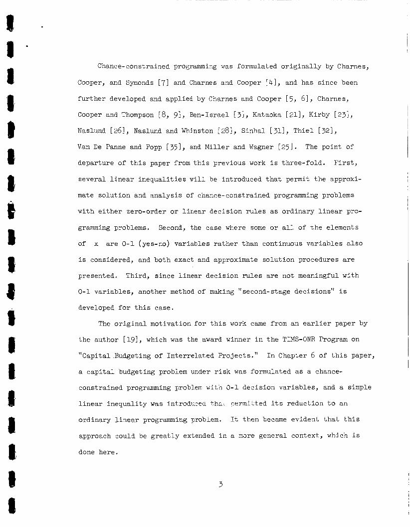
d i s t r i b u t i o n s or Poisson d i s t r i b u t i o n s , respec t ive ly . If t h e ind iv idua l ... random va r i ab le s have a r b i t r a r y d i s t r i b u t i o n s , then ,f a x - bi) may

s t i l l be approximately normal by some version of t h e Cent ra l L i m i t

i j j i j =1 Theorem, which holds under f a i r l y weak condi t ions for independent random

va r i ab le s and under r a t h e r s t rong condi t ions for dependent random va r i -

ab le s . A survey o f t h e var ious s e t s of condi t ions under which t h e

Cent ra l L i m i t Theorem holds i s given by t h i s author elsewhere [lg, Sect .

4.21. Whatever t h e d i s t r i b u t i o n of 1 F(*)

a i j x j - b ] happens t o be, l e t i \ J = 1 denote t h e cumulative d i s t r i b u t i o n func t ion of

Given B , 0 - - < l3 < 1, def ine % by t h e r e l a t ionsh ip ,

a Thus, by proceeding i n t h e usua l way, t h e de t e rmin i s t i c equivalent form

of t h e cons t ra in t becomes

which reduces t o

~

For example, see Cooper and Charnes E61 o r Kataoka [21] . Also see 8 H i l l i e r and Lieberman [ 201 f o r a d e t a i l e d exposi tory t reatment .

6

9 n 1 E ( a . .)x. + Ka X

i j =1 1 J J

The problem now i s t o reduce t h i s de t e rmin i s t i c equivalent form

f u r t h e r t o a more t r a c t a b l e farm,

t h e cons t r a in t s so t h a t l i n e a r programming and in t ege r l i n e a r program-

ming aigorithms can be used.,

following obvious r e s u l t ,

Fundamental Lemma: Assume t h e t gi (x) < g (x) < g (x) f o r a i l admis-

s i b l e x. Consider a solut ion x which i s f e a s i b l e i f and only i f

g2(xj _< k, ( i o e o , x s a t i s f i e s a l l o ther condi t ions f o r f e a s i b i l i t y ) .

The objec t ive w i l l be t o l i n e a r i z e

The bas i c approach i s suggested by t h e

I - 2 - 3

(i) If g,(x) 5 k, then x i s f e a s i b l e ,

(ii) If x i s f eas ib l e , t hen g,(x) < k ., - Thus,

form of t h e cons t ra in t , whereas

'resent l i n e a r cons t r a in t s t h a t a r e uniformly t i g h t e r acd uniformly

looser , respec t ive ly . These l i n e a r approximations w i l l be introduced

i n t h e next sect ion, and procedures f o r obtaining both exact and approx-

imately optimal so lu t ions ( i n i t i a l l y with zero-order dec is ion r u l e s and

g (x) < k 2 - w i l i represent some exact de te rminis t ic equivalent

x> < k and g,(x) < k w i l l rep- g,( - -

i s not. 91f t h e func t iona l form of the d i s t r ibu t . i on

known, so Ka,

y i e l d s

used here when

l-ai

i s not known, then t h e one- sided Chebyshev ' Inequal i ty

as an upper bound on I( a Eence, t h i s bound may be ai

i s not known i n order t o guarantee t h a t Kcxi

- bi> _> ai" (However, it should be noted that, t h e

bound i s based on t h e worst possible d i s t r i b u t i o n and therefore w i l l

u sua l ly overestimate Ka

s t r a i n t s t h a t a r e considerably t i g h t e r than necessal-y. )

grea t ly , so t h a t it would tend t o y i e l d con-

7

then w i t h o the r decis ion r u l e s ) w i l l then be described i n t h e succeeding

sec t ions.

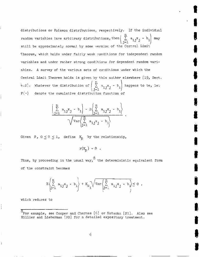
3. Useful Inequa l i t i e s n

j=l Consider again the t y p i c a l cons t r a in t , Prob { 1 a i jx j - bi - < 0

and i t s de te rminis t ic equivalent form given i n t h e preceding sec t ion .

Assume i n i t i a l l y t ha t

t h a t

ail, ... , ain, bi a r e mutually independent, so

- n

a? = Var(a 1, ( f o r i = 1, ... , m; j = 1, ... , n ) . I j i s

Theorem 1: Assume t h a t 0 < x . < 1 f o r j E C and x = 0 o r 1 f o r

j E D, and t h a t a

- J - j

... , ain, b a r e mutually independent. Then il' i

I 1 ' 1 B 1 Q 1 B

i s a

(iii)

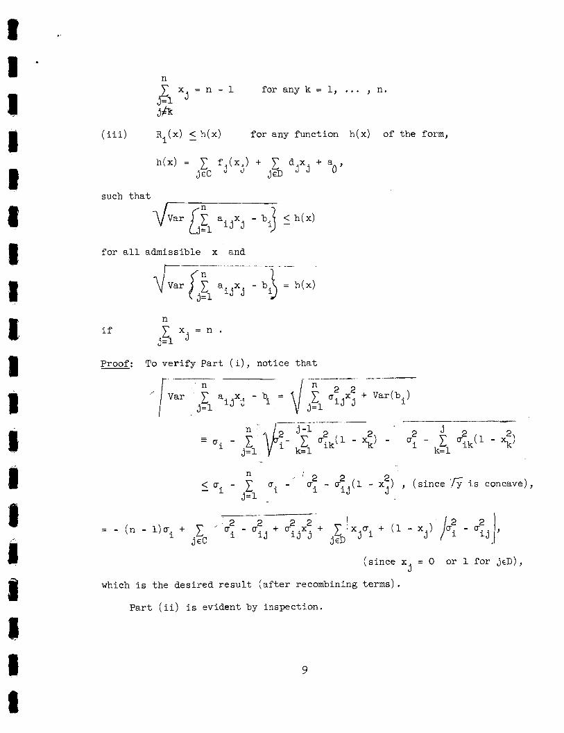
n 1 x j = n - l j=1 jh

for any k = 1, ... , n '

Ri(x) 1. h ( x ) f o r any funct ion h ( x ) of the form,

such t h a t

for a l l admissible x and

i f

Proof:

= - ( n

To v e r i f y P a r t ( i) , not ice t h a t

n n V a r 1 aijx3 - bi = + Var(bi)

J 2 2 , ( s i n c e '5 i s concave), < Ui - 1 ai - u - (1 - x . ) n

j= 1 i i j J -

+ u2.x2 + r - l ) u i + i j 1 J j

'IJ - 0 - i

j EC

( s i n c e x = 0 or 1 f o r jcD), J which i s the des i r ed r e s u l t ( a f t e r recombining te rms) .

P a r t (ii) i s evident by inspect ion.

9

n

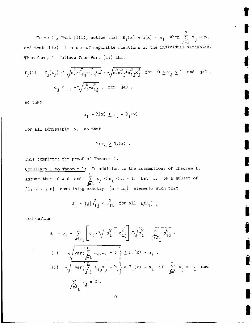
j=l To v e r i f y Pa r t (iii) , no t i ce t h a t R . ( x ) = h ( x ) = a i when x j = n, 1

and t h a t h ( x ) i s a sum of separable funct ions of t he ind iv idua l va r i ab le s .

Therefore, it follows from P a r t (ii) t h a t

a . J - a i -dx , f o r jcD ,

so t h a t

- h ( x ) < - u i - Ri(x) ‘i

f o r a l l admissible x, so t h a t

This completes the proof of Theorem 1.

Corol lary 1 t o Theorem 1:

assume t h a t C = Cp and 1 x j < n < n - 1. Let J1 be a subset of 1

(1, .. . , n) containing exac t ly ( n - nl) elements such t h a t

I n add i t ion t o the assumptions of Theorem 1, n

j=l

and def ine

ai = a i - 1 jcJl

I

and j= l

10

8 1 ' 1 1 1 9 1 s 11 1 1 11 8 f I si z 1 1

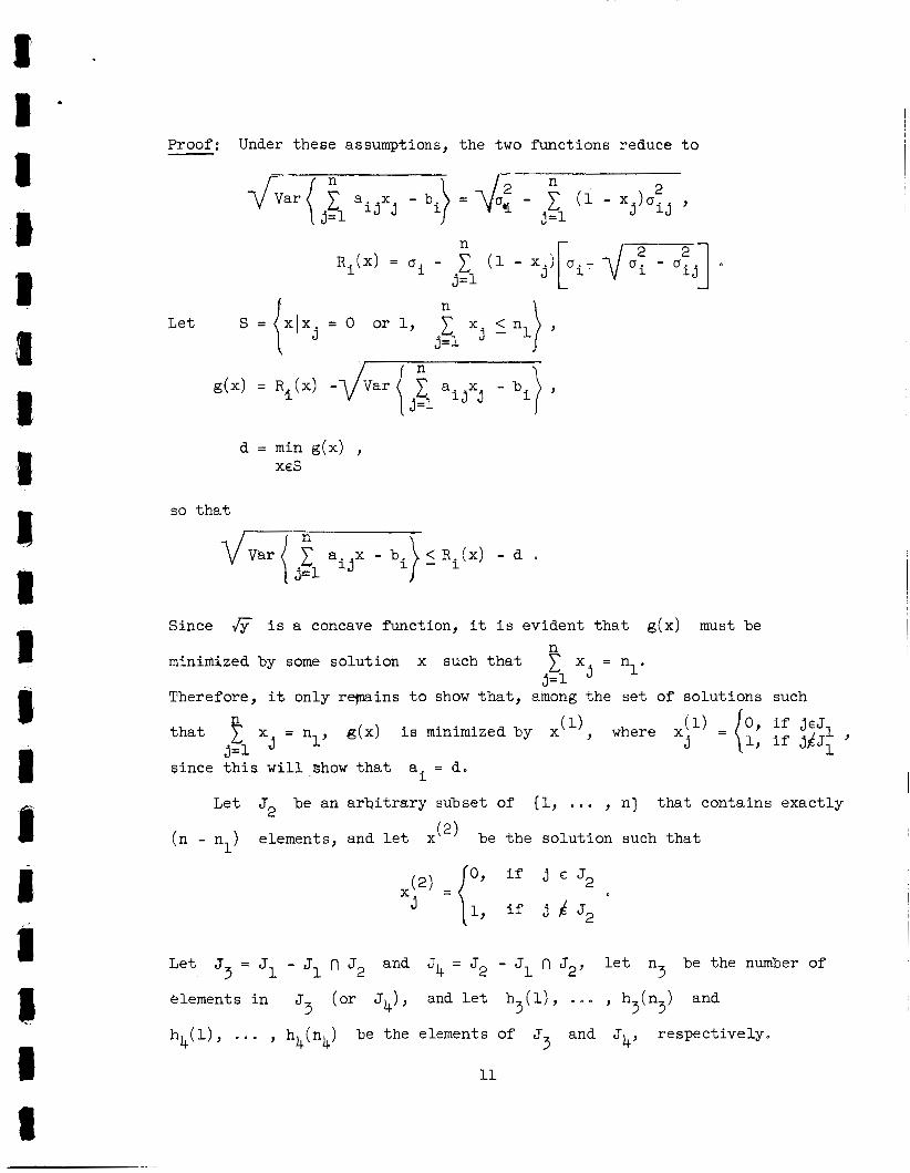
Proof: Under these assumptions, t he two func t ions reduce t o

d = min g(x) , X€S

so t h a t

Since fi i s a concave function, it i s ev ident t h a t g (x ) must be

minimized by some so lu t ion x such t h a t f x j = nl. J = 1 -

Therefore, it only repa ins t o show t h a t , among t h e s e t of so lu t ions such

(1) = {o, if' jcJ1 xJ 1, if jbJL ' t h a t f x j = nl, g(x) i s minimized by x"), where

j= l -

s ince t h i s w i l l show t h a t a = d o i

Let J2 be an arbitrary subset of (1, . o . , n) t h a t conta ins exac t ly

(n - nl) elements, and l e t x (2) be t h e so lu t ion such t h a t

0 , if j E J2

1, if J 1 J2

- - Jl n J2, l e t n be the number of Le t J = Jl - J1 n J2 and J - J 3

3 3

3 and l e t h 3 ( l ) , , h ( n ) and elements i n J3 (Or 54)'

h 4 ( l ) , , h (n be the elements of J3 and J4, respec t ive ly . 4 4 11

F i n a l l y , def ine

Therefore,

i j 2 2

i j

j -1

1 i j j=1

i j I \

s ince

nonnegative. This completes the proof .

fi i s a concave func t ion so t h a t each term i n t h e summation i s

1 ’ I I 1

12

t I

8 I 11 1 i I i 1

Corollary 2 to Theorem 1:

ing statements hold.

Under the assumptions of Theorem 1, the follow-

(i) Any so1ut;ion x that satisfies the set of constraints,

n

x = O or 1, for j e D ? j

necessarily is a feasible solution.

(ii) If the additional assumptions of Corollary 1 hold, then (i) will

still hold after replacing Ri(x) by [Ri(x) - ai] for i = 1, ?

, m, Ka > 0 and each nonlinear term (iii) If, for each i = 1, . O .

j u 2 - m2 + c2 x2 in R. (x) is approximated by a piecewise-linear

function that coincides with-&: - u2 + u x

and at the points where the slope of the piecewise-linear function changes,

- i

i ij ij j 1 2 2 only at x = 0, x = 1,

ij ij j s s

then both (i) and (ii) will still hold. Furthermore, each of these

piecewise -linear functions necessarily is convex n

j =1 (iv) Any feasible solution x such that 1 xs = n or

for any k = 1, ... , n necessarily satisfies the set of c

(i). Furthermore, if \ = 0 also, then this statement still must hold

after introducing the piecewise-linear functions described in (Lii)o

Proof: Given the Fundamental Lemma, all of these statements are an

immediate consequence of Theorem 1. The convexity of the piecewise-linear

functions described in (iii) is demonstrated simply by noting that

> o .

5 4 3 2 1 0

To gain some i n s i g h t i n t o the goodness of t he approximation introduced

10 10 9.487 9.487 8.944 8.974

7.746 7.948 7.071 7.435

8.367 8.461

by Theorem 1, consider a s an example a case where n = 5, E ( a . .) = 10 and

V a r ( a . .) = 10 for a l l j = 1, ... , 5, E(Bi) = 50 and Var (bi) = 50,

K = 2, and C = 0 . For t h i s case, the following numerical r e s u l t s a r e

obtained.

1 J

1 J

ai

I I 1

---- _____ -

70 58 * 974 47.888 36.734 25.492 14.142

-.

70 58 * 974 47.948

25.896 14.870

36.922

Thus, t h e approximation introduced by Theorem 1 i s exce l l en t here for the n

l a r g e r values of x j ,

which is where accuracy tends t o be important. j=1

Whereas t h e above r e s u l t s provide uniformly t i g h t e r cons t r a in t s ,

Theorem 2 below w i l l provide uniformly looser cons t r a in t s .

Theorem 2: Assume t h a t 0 < x < 1 f o r j E C and x = 0 or 1 f o r j E D ,

and t h a t a

- j l - a r e mutually independent. Then in’ bi

... a ( i)

( i) the re e x i s t s a unique r e a l constant v i’

Var ( b . ) + max {m:j) 5 vi 5 m2 such t h a t 1 i y

j E ( 1 , ..., n)

14

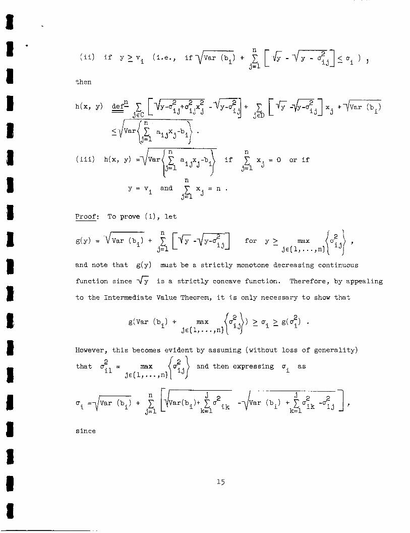
then

y = v and i

Proof: To prove ( i) , l e t

and note t h a t g (y ) must be a s t r i c t l y monotone decreasing continuous

funct ion s ince 6 i s a s t r i c t l y concave funct ion. Therefore, by appealing

t o t h e Intermediate Value Theorem, it i s only necessary t o show t h a t

However, t h i s becomes evident by assuming (without loss of gene ra l i t y )

t h a t ui1 2 = max Pj} and then expressing cr as i j c ( 1 , . . . ,n)

s ince

> - a i --JK 4

To prove (ii), note t h a t , f o r f i xed x, h(x , y) i s a s t r i c t l y

monotone decreasing func t ion of y. Thus, it i s s u f f i c i e n t t o prove (ii)

2 f o r y = v It w i l l now be assumed t h a t D = i i n j c ( 1 , ..., n)

F i r s t consider the case where

Then

Now consider t h e complementary case where

2 n-1 = Var (b i ) + m:kxE + ain . k= 1

16

Then

which completes the proof of (ii)

P a r t (iii) i s evident by inspect ion.

Corol lary t o Theorem 2:

statements hold.

Under t h e assumptions of Theorem 2, the following

( i ) If ui < v i f o r a l l i = 1, . O . , m, then any f e a s i b l e so lu t ion - x n e c e s s a r i l y s a t i s f i e s t he s e t of cons t ra in ts ,

O < x - < l , for j c C , - 3 -

x J = O or 1 , f o r j E D .

j=1 (ii) h(x,cri) 2 = Ri(x) + (n-l)Ui -

(iii) If, fo r each i = 1, o . o , m, K > 0 and each nonlinear term

d m i n h(x, u . ) i s approximated by a convex piecewise- :

- 9 i j j 1

~~

l i n e a r funct ion t h a t never exceeds ’/ui - crTj + C;~X;,’ then (i) w i l l s t i l l

hold.

( i v ) Any so lu t ion x t h a t s a t i s f i e s the s e t of cons t r a in t s i n (i) n

n e c e s s a r i l y i s a f eas ib l e solut ion i f c x j = 0 , or i f u = v i i

n .j=1 ( f o r i = 1, ... , m) and 1 x j = n o -

.1=1

Although no e x p l i c i t so lu t ion f o r t he vi has been given, they can be

I r e a d i l y determined (wi th in a spec i f i ed e r r o r ) by standard numerical methods

n

j= l

5 L 9 414 3 8 828 2 8.243 1 7 657 0 7 "071

h(x , v ' i' c xj 10

s ince h(x , y) i s a s t r i c t l y mmotone decreasing func t ion of y o

n 2 E ( a i J \ x * K j=l

h ( x , vi) j ai

70 58 828 47 656 36,486 25 31k 14 142

To i l l u s t r a t e t h e app i i ca t i cn of Thewem 2, c m s i d e r again the numerical

example introduced following Theorem 1- For t h i s case, fiy -dqT =

0,5858 (so vi = 77.941, which y i e l d s t h e following r e s u l t s o

i 9

I I f n -l

, Comparison with the and

[ j f 1 J J ai t h i s i s an exce l len t "uniformly looser" l i n e a r approximation,

E ( a . . ) x . + K given e a r l i e r indicat,e t h a t

, a in j b i a r e no t mutually i j ' Now consider t h e case where a

I I independent, so tha t

I n n n I 2 n

= x V a r ( a . . ) x . + Var(bi) f 1 2 L"ov(a ij' a i k ) x J x k - j=l Cov(a i j ,b i )x . J . j=l 1 J J k = l j = l

kf j

Lemma 1: Define

- 2 ~ o v ( a i j J a i k ) - E(aik)D(aik), f o r J,k = 1, 1 1 n (k#J) , ai B i j k -

18

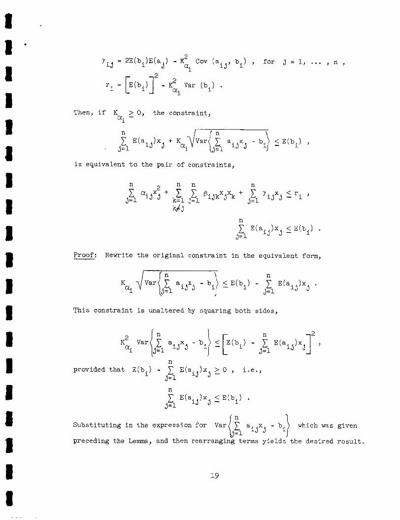
2 r i = [E(bi)] - Ci Var (bi) .

Then, if K > 0, t h e cons t ra in t , - ai

i s equivalent t o t h e p a i r of cons t r a in t s ,

n h n n n

Proof: Rewrite t h e o r i g i n a l cons t ra in t i n t h e equivalent form,

1 f n \ n

T h i s cons t r a in t is unal te red by squaring both s ides ,

n

j=1 provided t h a t E(bi) - 1 E(a . ) X . > 0 , i . e .9

l j J - n 1 E(aij!x < E ( b i )

j= l j -

S u b s t i t u t i n g i n t h e expression f o r V a r 1 a i j x j - bi) which w a s given

preceding the Lemma, and then rearranging terms y ie lds t h e des i red r e s u l t , (" j=l

1

n n n ( i t ) 1 1 pijkxjxk = ui(x) i f 1 x j = n , o r i f

k = l j = l j = l

n 1 x j = n - 1

j = l < 0 f o r a l l j , k = 1, ".. , n ( k f j ) and p i j k -

for any k = 1, . . e , n , or i f pijk 2 0 f o r a l l

n j , k = 1, . o e , n ( k f j ) and 1 x j = 0

j=1

(iii) If p < 0 f o r a l l j , k = 1, , n ( k f j ) , i j k -

then U.(x) < - h(x) f o r any func t ion 1

h ( x ) of the form, n

such t h a t n n

f o r all admissible x and

n n

n

j=l i f 1 x j = n .

20

I I E

1 I 1 1 t I B il

Proof: To prove ( i ) , observe t h a t

n n n n

n n n n

it fol lows t h a t

n n 1 n -1 1 @ijkXk 1 ii-x.) J k = l

n n n r n

as was t o be shown.

P a r t (ii) i s ev ident by inspect ion, and (iii) follows immediately from (ii).

Corol la ry 1 t o Theorem 3 : I n add i t ion t o t h e assumptions of Theorem 3, assume

B i j p j ( 2 ) 2 @ i j p . ( n - I ) . Define J

n n n

2 1

(ii) Define A (B i jk + min {Bi jk f 011 , f o r j = l , . . * , n , and

l e t si be t h e sum of the (n-n,) smallest elements of (Ail,. . . ,A. i n ) . & n

Then & 1 pijkxjxk 5 Ui(xj - S i *

k f j j= l Proof: The key s tep i s t o note t h a t

n n n

n -1 f n-1 f

P a r t ( i ) then follows immediately by using the expression obtained i n the

proof of Theorem 3,

n n

n A f t e r no t ing t h a t A > 0 f o r a l l j and t h a t 2 (1-x . ) > (n-nl),

P a r t (ii) then follows from P a r t (i).

i j - J - j= l

Corol lary 2 t o Theorem 3:

( i ) Any solut ion x t h a t s a t i s f i e s t h e se t of c o n s t r a i n t s ,

n - n 2

j = l 1 J j 1 a. .X + ui(x) + 1 yijxj - < r i ' f o r i = 1, . o * , m , j = l

O < x . < 1 , f o r j E C , - J -

X = 0 o r l , f o r j E D , J

necessa r i ly i s a f e a s i b l e so lu t ion .

22

(ii) If t h e a d d i t i o n a l assumption of Corol la ry 1 holds, then ( i) w i l l n n n

s t i l l hold a f t e r replacing U . ( x ) by e i t h e r pijk- 1 e . . ( l - x . )

J 1 1 j=1 'J 7 ma or [u i (x ) - s i ] f o r i = 1, ...

(iii) If C = @, then both ( i) and (ii) w i l l s t i l l hold a f t e r rep lac ing

9 by x j f o r j = 1, ... 2 xJ

( i v ) Assume t 'nat C f 0 and t h a t , f o r i = 1, ... , m, aij >_ 0 fo r each

3' j E C . Suppose t h a t , fo r each j E D, x2 i s rep laced i n ( i ) by x j -

2 and t h a t , f o r each j E C , x i s approximated i n ( i) by a piecewise-

l i n e a r func t ion t h a t coincides with x only a t x = 0, x. = 1,

and a t t h e po in t s where t h e slope of t h e piecewise- l inear func t ion

j 2 j j J

changes ( s o t h a t t h i s piecewise- l inear func t ion necessa r i ly i s convex).

Then both ( i ) and (ii) w i l l s t i l l hold.

( v ) A f e a s i b l e so lu t ion x necessa r i ly s a t i s f i e s t h e s e t of c o n s t r a i n t s i n n LI

(i) i f (I.) 2 x = n, o r (2)pijk < 0 f o r a l l j , k = 1, . D O , n ( k f j ) - j - n j =1 and

j , k = 1, ... , n(k# j ) and c x = 0. Furthermore, i f x = 0

a l s o i n condi t ion ( 2 ) , then t h i s e n t i r e statement s t i l l must hold

x j = n-1 f o r any k = 1, .. . , n, or (3) pijk < 0 for a l l j= - Jfk n

j k j=1

a f t e r making t h e changes descr ibed i n ( i v ) .

Proof: Given t h e Fundamental Lemma and Lemma 1, these s ta tements a r e an

immediate consequence of Theorem 3 and Corol la ry 1.

Theorem 4: Assume t h a t 0 < x. < 1 f o r j E C , x = 0 or 1 f o r j E D, - J - j n < n Define p . ( k ) as i n Corol la ry 1 t o Theorem 3 , and l e t

J and no 5 x j - 1' J=1

1 0 I n -1 n

, n e + c max i p i j p e ( h ) ' O ) , f o r j = 1, J 0 k= n 'lj = 1 p i j p . ( k )

k= 1 J

23

Then n n n

24

n Proof: Note t h a t 1 pijkXk 5 Yfjxj7 so t h a t

k= 1

n n 1

kfJ Lkf j J n

j = l < - 1 Y f j X j 7

as w a s t o be shown.

Corol lary t o Theorem 4: Af te r imposing the assumptions of Theorem 4,

Statement ( i ) and i t s extensions i n Statements (iii) and ( i v ) of Corol lary

2 t o Theorem 3 w i l l s t i l l hold a f t e r rep lac ing Ui(x) by y ! .x n

j = l 1 J j

The decis ion whether t o use Theorem 3 o r Theorem 4 t o ob ta in a l i n e a r n n

upper bound on 6 n k f j

of 1 x j .

t end t o be r e l a t i v e l y t i g h t if 1 xj i s r e l a t i v e l y c lose t o n . However,

pijkxjxk depends l a r g e l y on t h e a n t i c i p a t e d values k= j=

The bounds provided by Theorem 3 and Corol la ry 1 t o Theorem 3 j = l n

.i=1 n "

i f t h e i n t e r e s t i n g f e a s i b l e so lu t ions tend t o y i e l d va lues of x j t h a t j = l

a r e r e l a t i v e l y small with r e spec t t o n, then the bound provided by Theorem

a r e 4 may be b e t t e r , e s p e c i a l l y i f (nl - no) i s no t l a r g e and the @i j k

no t t oo va r i ab le . To i l l u s t r a t e , consider once again the numerical example

introduced a f t e r Theorem 1, arrd impose the a d d i t i o n a l r e s t r i c t i o n t h a t I1

2 5 x j 5 3. Thus, ai j = - 60, @i j k = - 100, y i j = 1000, r i = 2300, .1=1 "

e = - 700, s = - 200, and y I = - 100 f o r a l l j , k , which y i e l d s i j i I j

t h e following r e s u l t s

21 *bpi jkxjxk, Whereas both Theorems 3 and 4 provided upper bounds on k=: J = k& .i

Theorem 5 below w i l l provide a l i n e a r lower bound on t h i s funci ion.

Theorem 5: Assume t h a t 0 < x. < 1 for j E C, x = 0 or 1 f o r j E D ,

and n < x j 5 nl. Define p j ( k ) as i n Corollary 1 t o Theorem 3, l e t n - J - j

0 - J =

! n p if j C and let

n -1 N

I \, for j = 1, , n 0 j

k= 1 1 ' i jp . (n-k) J + k=n 1 min \ ' i jpj(n-k) ' 'ij' 0

Then

n n n

( i t ) 2 qi jxj = 1 BijkXjXk if 1 x j = o a

j= l k = l j=1 j=1 k# j

Proof: Note t h a t

so t h a t r- 1

This ve r i f i e s ( i ) , and (ii) i s obvious by inspect ion.

25

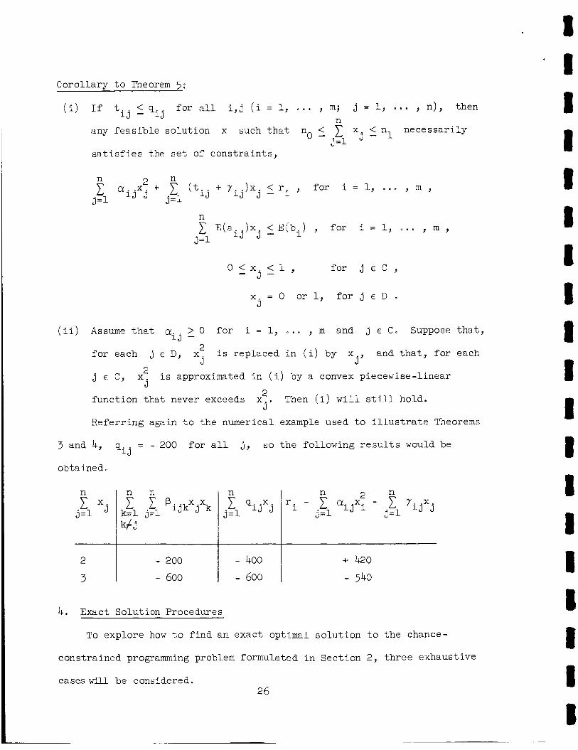
I Corol lary t o Theorem 5:

- 400 - 600

( i ) If t i j 5 q i j f o r all i , j ( i = 1, a . . , m; n

j=1

j = 1, ... , n ) , then

any f e a s i b l e so lu t ion x such t h a t no 5 1 x j nl necessa r i ly

s a t i s f i e s the s e t of cons t r a in t s ,

+ 420

- 540

0 < x . < 1 , f o r j E C , - J -

x = O o r l , f o r j E D . 3

(ii) Assume t h a t ai j > - 0 f o r i = 1, , m and j E C. Suppose t h a t ,

f o r each j E D, x2 i s replaced i n ( i ) by x and t h a t , f o r each

j E C ,

func t ion t h a t never exceeds x e Then ( i) w i l l s t i l l hold.

Refer r ing again t o the numerical example used t o i l l u s t r a t e Theorems

J j '

x2 i s approximated i n ( i ) by a convex piecewise- l inear j

2 j

3 and 4, q; = - 200 f o r a l l j , so t h e fol lowing r e s u l t s would be

ob t a ine d

n

j = l C x j

2

3

n n

k=l j=1 -1 ' ijkXjXk

0 < x . < 1 , f o r j E C ,

x = O o r l , f o r j E D .

- J -

3

(ii) Assume t h a t ai j > - 0 f o r i = 1, , m and j E C. Suppose t h a t ,

f o r each j E D, x2 i s replaced i n ( i ) by x and t h a t , f o r each

j E C ,

func t ion t h a t never exceeds x e Then ( i) w i l l s t i l l hold.

Refer r ing again t o the numerical example used t o i l l u s t r a t e Theorems

J j '

x2 i s approximated i n ( i ) by a convex piecewise- l inear j

2 j

3 and 4, q; = - 200 f o r a l l j , so t h e fol lowing r e s u l t s would be

ob t a ine d

n

j = l C x j

2

3

4. Exact Solut ion Procedures

To explore how t o f i n d an exac t optimal s o l u t i o n t o t h e chance-

cons t ra ined programming problem formulated i n Sec t ion 2 , t h r e e exhaust ive

cases will be considered. 26

~~~

- 200

- 600

4. Exact Solut ion Procedures

To explore how t o f i n d an exac t optimal s o l u t i o n t o t h e chance-

cons t ra ined programming problem formulated i n Sec t ion 2 , t h r e e exhaust ive

cases will be considered. 26

F i r s t , suppose t h a t D = c p , so t h a t a l l of t h e dec is ion v a r i a b l e s

a r e continuous v a r i a b l e s . Kataoka [21, pp. 194-53 has shownl0 t h a t

X i s a convex funct ion. Therefore, i f K > 0 f o r ai -

i = 1, . . o , my it i s known t h a t t h e de t e rmin i s t i c equivalent form of

the problem i s an ordinary convex programming problem, f o r which the re

e x i s t s a number of algorithms. These include t h e ones developed by Rosen

[3O], Zoutendigk [ 3 8 ] , Kelley [22] , and Fiacco and McCormich [13, 141.

Now consider t he case where C = c p , so t h a t a l l of t h e dec is ion

va r i ab le s a r e constrained t o be e i t h e r 0 o r 1, This case may be

solved i n a s t ra ight-forward manner a s follows. F i r s t , r ep lace t h e

de t e rmin i s t i c equiva len t form of t h e s e t of cons t r a in t s by a s e t of

uniformly t i g h t e r l i n e a r cons t r a in t s . If i t s assumptions a r e s a t i s f i e d ,

such s e t s a r e i d e n t i f i e d by P a r t s ( i) and (ii) of Corol lary 2 t o Theorem

1,

2 t o Theorem 3 o r the Corol lary t o Theorem 4.

Otherwise, use one of t he s e t s i d e n t i f i e d by P a r t (iii) of Corol lary

Then f i n d a good suboptimal

so lu t ion t o the r e s u l t i n g in teger l i n e a r programming problem, which may be

done by us ing one of t he suboptimal algorithms developed by t h e author [18],

This so lu t ion necessa r i ly i s f e a s i b l e f o r t h e o r i g i n a l problem. Next,

rep lace t h e de t e rmin i s t i c equivalent form of t h e o r i g i n a l cons t ra . in t s by a

s e t of uniformly looser l i n e a r c o n s t r a i n t s , Such a s e t may be obtained

from the Corol lary t o Theorem 2, i f i t s assumptions hold, o r from t h e

Corol la ry t o Theorem 5. This y i e l d s an ordinary in teger l i n e a r program-

ming problem whose s e t of' f e a s i b l e so lu t ions includes a l l so lu t ions t h a t

a r e f e a s i b l e f o r the o r i g i n a l problem, The f i n a l s t ep i s t o apply a

l0Also see S inha l [31] and Van de Panne and Popp [35, pp. 421-21 f o r r e l a t e d inves t iga t ions .

27

s l i g h t l y modified vers ion of a bound-and-scan algori thm developed by t h e

author [l?] f o r the in teger l i n e a r programming problem. Given a good

f e a s i b l e so lu t ion , t h i s a lgsr i thm repea ted ly f inds success ive ly b e t t e r

ones u n t i l an optimal so lu t ion i s reached. Therefore, t h e one modif icat ion

t h a t i s requi red i s that , a new " b e t t e r f e a s i b l e so lu t ion" should be d i s -

carded i f it i s not f e a s i 5 l e f o r the o r i g i n a l problem, The f i n a l so lu t ion

y ie lded by t h i s modified algori thm w i l l then be the optimal so lu t ion t o the

o r i g i n a l problem.

F ina l ly , consider t he genera l case where the re e x i s t both continuous

and in teger decis ion va r i ab le s This problem i s considerably more d i f f i -

c u l t than the spec ia l cases discussed above. However, i f K > - 0 f o r

i = 1, e o c , m, then an algori thm r e c e n t l y developed by Veinot t [ 3 6 ] i s ai

app l i cab le , Although i t s scmpu%ational e f f i c i e n c y i s untes ted a t p resent ,

t h i s a lgori thm i n p r i n c i p l e w i l l converge t 3 the optimal so lu t ion f o r t h i s

pr ob lem

5. Approximate So lu t io r Procedures

Despite t h e a v a i l a b i l i t y of the exact so lu t ion procedures descr ibed

above, approximate procedures t h a t expedi te computation and s e n s i t i v i t y

a n a l y s i s a l s o a r e of considerable p r a c t i c a l i n t e r e s t . Such procedures

w i l l be described below, To c l a r i f y the expos i t ion , t h e requirement t h a t

x = 0 or 1 ra the r than 0 < x . < 1. f o r j E D w i l l be ignored u n t i l

t h e l a t t e r p a r t of t h e sec t ion , j - J -

A good " d e f i n i t e l y f eas ib l e" so lu t ion may be obtained r e l a t i v e l y

e a s i l y by applying the r e s u l t s given i n Sec t ion 3 0 The f i r s t s t e p i s t o

rep lace t h e de te rminis t ic equivalent form of t h e s e t of c o n s t r a i n t s by a

s e t of uniformly t i g h t e r piecewise- l inear c o n s t r a i n t s . This new s e t may

28

be se lec ted from any of those provided by P a r t (iii) of Corollary 2 t o

Theorem 1, P a r t s (iii) and ( iv) of Corollary 2 t o Theorem 3, and the

Corollary t o Theorem 4 f o r which the assumptions hold.

so lu t ion t o t h i s new problem i s the desired " d e f i n i t e l y f eas ib l e" so lu t ion .

I t may be obtained by converting the problem t o an ordinary l i n e a r program-

ming problem by the well-known separable convex programming technique

(e .g . , see Hadley [16, Ch. 41) and then solving it by a streamlined

vers ion of t he simplex method.

s c r ibes how t o use t h e decomposition p r i n c i p l e t o s implify the computa-

t i o n a l procedure.

The optimal

For example, Hadly [16, pp. 126-91 de-

The above approach i s a conservative one i n t h a t many "barely

f eas ib l e" so lu t ions a r e excluded from consideration. I t i s n ' t always

des i rab le t o be t h i s conservative, e s p e c i a l l y s ince the a of ten represent

only rough guidel ines t h a t were s e t on a subject ive b a s i s , An opposite

approach would be t o consider a l l f ea s ib l e so lu t ions plus some "barely

infeas ib le" ones.

t h a t the new s e t of cons t ra in ts would be se lec ted from those provided by

P a r t (iii) of the Corol lary t o Theorem 2 or P a r t (ii) of the Corollary t o

Theorem 5 . T h i s w i l l provide a so lu t ion which y i e l d s a value f o r t he

object ive funct ion t h a t i s a t l e a s t a s la rge as t h a t f o r the optimal

so lu t ion but which may not be qui te f e a s i b l e f o r t he given values of t he

i

This may be done by proceeding exac t ly a s before except

?Lo

Another approach t h a t may be more s a t i s f a c t o r y i s t o combine the above

two. One way t o do t h i s i s t o search f o r the b e s t f e a s i b l e so lu t ion along

the l i n e segment between the "de f in i t e ly feas ib le" so lu t ion and the "nearly

f eas ib l e" so lu t ion described above, Another way i s t o search f o r t h e .best

f e a s i b l e so lu t ion yielded by using a weighted average of the two s e t s of

29

t

cons t , ra in ts* If these two s e t s d i f f e r only i n t h e r ight-hand s ide of t h e

respec t ive cons t ra in ts , then the so lu t ions may be obtained e a s i l y by

standard parametric programming procedures ( e , g . , see H i l l i e r and

Lieberman [ 20 ] ) li

S t i l l another approach i s to use the so lu t ion obtained i n any of t h e

above ways t o construct a b e t t e r s e t of a.pproximate l i n e a r cons t r a in t s ,

which a r e then used t o f i n d the f i n a l so lu t ion . For example, l e t

x* = [x*, o o c , x:lT %e the " d e f i n i t e l y f eas ib l e" so lu t ion descr ibed

above, Then one may replace

i n Lemma 1 and use t h e r e s u l t i n g p a i r of cons t r a in t s t o rep lace t h e

1 n n n n

k& ;& 'ijkXjXk by -< [& 'ijk%]x j k$J J=

corresponding o r ig ina l cons t r a in t f o r each i = 1, , n. A l t e rna t ive ly ,

t he s e t of cons t ra in ts descr ibed i n Corol lary 2 t o Theorem 1 may be

modified by replacing Ri(x) b y

' 1 \

n - L

l o r each i = 1, ... , m, where v = Var { ,I a i j X J - bi; and di i s i J=1

I

l h o ~ t h i s case, an upper bound on t h e d i f fe rence between t h e va lue of t he

objec t ive function f o r the optimal so lu t ion and the se l ec t ed so lu t ion may

be obtained e a s i l y a s fol lows, Let M be the number of func t iona l con-

s t r a i n t s , and l e t be the optimal dua l so lu t ion co r re -

sponding t o t h e se lec ted pr imal so lu t ion . Let Abi 'be the d i f f e rence

between the right-hand s ide of t he ith func t iona l cons t r a in t f o r t h e

' b r l y f eas ib l e" so lu t ion descr ibed above and t h a t f o r t h e s e g c t e d

(See t h e sec t ion e n t i t l e d "Bounding Procedure f o r Group 3 and 4 Variables"

i n [l7] f o r t h e j u s t i f i c a t i o n of t h i s r e s u l t . ) I n general , t h e value of

t he objec t ive funct ion f o r t he "Eearly f eas ib l e" s o l u t i o n a l s o provides an

upper bound on the corresponding value f o r the optimal so lu t ion .

[q, y ( I D ,

so lu t ion , where i = 1, M, Then t h i s upper bound i s q q A b i . i=

30

* I I 8 8 I 8 1 I I I I 8 1 i 1 1 1 8

the constant required t o make t h i s new funct ion equal t o - & V w

when x = x*. For e i t h e r case, one would then apply the separable convex

programming technique and solve as before . It appears t h a t t h e r e s u l t i n g

so lu t ion should tend t o be near ly optimal and e i t h e r f e a s i b l e or s u f f i c i e n t l y

c lose t o f e a s i b l e f o r most p r a c t i c a l purposes.

All of the above approximate procedures reduce t o solving a l i n e a r

programing problem. This has important advantages over t he exact so lu t ion

procedures described in t h e preceding sec t ion .

e f f i c i e n c y w i t h which a l i nea r programming problem can be solved o r i g i n a l l y

and then subjected t o s e n s i t i v i t y ana lys i s . Another advantage i s the

a v a i l a b i l i t y of l i n e a r dua l i t y theory f o r analyzing the problem,

optimal dual solut ion, which i s an automatic by-product of the ordinary

l i n e a r programing calculat ions, i s a v a i l a b l e f o r fu r the r guidance and for

study of the o r i g i n a l po l icy decis ions made when construct ing the chance-

constrained programming model.

One i s the r e l a t i v e l y high

Thus the

Now consider how t o d e a l with v a r i a b l e s t h a t a r e r e s t r i c t e d t o be

e i t h e r 0 or 1. The l i n e a r programming so lu t ion procedures described above

may ass ign f r a c t i o n a l values t o some of these var iab les , so t h a t some

modification i s required. "he simplest approach i s t o attempt t o round

such v a r i a b l e s up or down i n such a way as t o obtain a f e a s i b l e so lu t ion

with a r e l a t i v e l y la rge value of the objec t ive funct ion. Fortunately,

according t o a theorem due t o Weingartner [37, pp. 35 f f . ] , t he number of

f r a c t i o n a l v a r i a b l e s i n these l i n e a r programming so lu t ions cannot exceed

the number of funct ional cons t ra in ts . Therefore, i f m i s not la rge ,

t h e r e can only be a r e l a t i v e l y f e w v a r i a b l e s t h a t w i l l need ad jus t ing .

Furthermore, since t h e f i n a l so lu t ion needs t o be f e a s i b l e only f o r t h e

o r i g i n a l problem, and not, f o r t h e approximating l i n e a r programing problem,

it may be possible t o increase t h e value of t he object ive funct ion over

t h a t f o r t h e optimal l i n e a r programming solution^

A more systematic approach t o t h e in t ege r or mixed in t ege r problem i s

t o formulate a n approximating l i n e a r programming problem as described above

and then apply one of t h e a v a i l a b l e algorithms f o r t h e pure in t ege r or

mixed in t ege r programing pro-blem ( s e e Bal inski [l] and Beale [ 2 ] f o r a

survey of t h e s e algori thms) .

than can be j u s t i f i e d , e s p e c i a l l y consider ing t h a t t h e r e s u l t i n g so lu t ion

need not be optimal f o r t he o r i g i n a l problem, A more e f f i c i e n t procedure

i s t o in s t ead apply a suboptimal i n t ege r programming algorithm, such as

those developed by R e i t e r and Rice [ 2 9 ] and ( i f

The Reiter-Rice algorithm a l s o can be appl ied d i r e c t l y t o t h e o r i g i n a l

problem i n i t s de t e rmin i s t i c equivalent form, which should tend t o y i e l d a

s l i g h t l y b e t t e r so lu t ion with somewhat l e s s e f f i c i e n c y .

6. Linear Decision Rules f o r Continuous Variables

However, it may r e q u i r e more computation t i m e

C = c p ) by t h e author [18].

Now consider t h e s i t u a t i o n where the values taken on by c e r t a i n of

t h e random v a r i a b l e s w i l l become known before some of t h e dec i s ion v a r i a b l e s

must be assigned v a l u e s , I t i s h ighly d e s i r a b l e t o formulate and solve

problems of t h i s type i n such a way t h a t t h e u l t ima te dec i s ions w i l l be

p a r t i a l l y based on t h e new information t h a t has become a v a i l a b l e .

i nd ica t ed i n Section 1, one way t o do t h i s i s t o formulate t h e problem i n

terms of choosing a decis ion r u l e ,

As

x = q(A, b, C ) e

where i s a vector-valued func t ion t o be determined.

32

.

T h i s approach becomes quite t r a c t a b l e when i s r e s t r i c t e d t o the

c l a s s of l i n e a r decis ion ru les . I n p a r t i c u l a r , l e t t he components of be

m n m % = 1 uijkaij + vikbi + wk , fo r k = 1, , n ,

i=l j = l i=l

and v a r e decision v a r i a b l e s , except t h a t they a r e s e t i j k i k where u

equal t o zero i f k E D o r i f x must be assigned a value before k

observing a and b respect ively; w i s a decis ion v a r i a b l e i f

k E D or i f x must be assigned a value before observing any of t he

i j i’ k

k

a and bi, and it i s an a r b i t r a r y constant otherwise. i j

Since a general l i n e a r decision r u l e may ass ign a value other than

0 or 1 t o \, it has been necessary t o reserve these r u l e s f o r only

the continuous dec is ion var iab les . Therefore, i f k E D, then 5 = wk

only so t h a t it does not depend on t h e values taken on by the

An a l t e r n a t i v e approach t h a t does permit defer r ing 0 - 1 decis ions w i l l

a and bio i j

be described i n the next section.

To solve t h e chance -constrained programming problem with the ind ica ted

l i n e a r decis ion r u l e , no t ice t h a t

n n r m n m 1

n m n n m n

and, s imi la r ly ,

33

Therefore, i f t h e c a r e s t a t i s t i c s l l y independent of the a i j and bi,

and i f t h e r e s t r i c t i o n t h a t dec is ion va r i ab le s l i e between 0 and 1 i s

ignored, then t h e o r i g i n a l model reduces t o

k

subjec t t o

I n m n n m n

, f o r t = 1, O D . , m

w = O or 1, f o r k c D . k

"k Note t h a t t he decis ion va r i ab le s here p lay the same r o l e t h a t t h e

played before w i t h the zero-order dec is ion r u l e , S imi la r ly , t he co r re -

sponding ( a t k a i j t k J t k

a before . Therefore, except f o r two added complications, one m y

proceed e x a c t l y as before t o solve f o r t he dec is ion v a r i a b l e s .

complications a r e (1) it i s now more d i f f i c u l t t o determine t h e expectat ion,

var iance, and covariance terms, and (2 ) t he requirement t h a t t h e dec is ion

va r i ab le s must l i e between 0 a.nd 1 s t i l l remains t o be taken i n t o account.

The remainder of t h e s ec t ion w i l l be devoted t o d iscuss ing these two

) , ( a b . ) , and a now p lay t h e same r o l e as t h e

t k

These

complications.

To i l l u s t r a t e t h e former complication, consider how one would f i n d the

expectat ion, variance, and covariance terms involving only (" tkai j ) '

Assume t h a t t h e elements of A and b a r e mutually independent, t h a t t he

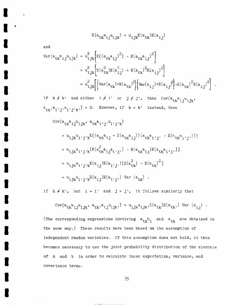
expected value and var iance of t hese elements a r e known, and t h a t uikk = o f o r a l l i and k , Then

34

8 . I ' I I I 8 8 1 I 8 I t I 8 I 8

1 1

e

If k f k' and either i f i' or j f jl, then Cov(atkaijuijk,

atkla~ljluiljlkl ) = 0. However, if k = k' instead, then

If k f kl, but i = it and j = jl, it follows similarly that

(The corresponding expressions involving a b and a are obtained in

the same way.)

tk i tk These results have been based on the assumption of

independent random variables. If this assumption does not hold, it then

becomes necessary to use the joint probability distribution of the elements

of A and b in order to calculate these expectation, variance, and

covariance terms.

35

Now consider the former requirement t h a t bounds of 0 and 1 be

If the objec t ive i s t o obta in an imposed upon t h e decisioR va r i ab le s .

optimal decis ion ru le by t h e so lu t ion procedures descr ibed i n Sect ion 4,

then these lower and upper bound c o n s t r a i c t s play no e s s e n t i a l r o l e and

can be omitted sa fe ly , However, t h i s i s not the s i t u a t i o n i f an approx-

imate dec is ion ru le i s being solAght by means of the i n e q u a l i t i e s presented

i n Sect ion 3, since these i n e q u a l i t i e s a r e based c r i t i c a l l y on the v a r i a b l e s

ly ing between 0 and 1- Therefore, it i s necessary f o r t h i s case t h a t

t h e cur ren t decis ion va r i ab le s be so constrained, although t h e so lu t ion

procedure would not r equ i r e t h a t the replaced v a r i a b l e s - t h e

between these bounds. However, unless appropr ia te adjustments a r e made,

xk - l i e

and v may e l imina te i j k i k a r b i t r a r i l y imposing such cons t , ra in ts on t h e u

i n t e r e s t i n g decis ion r u l e s from considerat ion. These adjustments a r e

discussed below,

One may e s s e n t i a l l y insure t h a t a l l of t he i n t e r e s t i n g values of t he

and v are nonnegative merely by a s s ign ing s u f f i c i e n t l y small i j k i k U

(poss ib ly negative) values L O each w t h a t i s not a dec is ion v a r i a b l e .

A s ca l ing f a c t o r may then be used t o e s s e n t i a l l y in su re t h a t t hese

k

i n t e r e s t i n g values do not exceed one. I n o ther words, each a (and bi) ij

(sad v ) would be mul t ip l i ed and divided, i j k i k and the corresponding u

respec t ive ly , by a s u f f i c i e n t l y l a rge constant ( n o t necessa r i ly the same

and v without i k

f o r a l l a and b i ) - This scslles down t h e u i s i j k

changing the problem, Af t e r s u f f i c i e n t t r a n s l a t i o n and change of s ca l e of

t h e decis ion var iab les , t h e lower and upper bmnd c o n s t r a i n t s may be

imposed without s e r ious ly reducing the s e t of f e a s i b l e so lu t ions

35

‘ I I 8 8 I 8 I I I I I 1 I 1 8 I 8 8

This process of t r a n s l a t i n g and s c a l i n g the decis ion v a r i a b l e s may be

conducted somewhat by t r i a l and e r r o r . For example, a t r i a l approximate

so lu t ion might be obtained a f t e r a modest amount of sca l ing . I f many of

t he v a r i a b l e s i n t h i s solut ion equal one, it would then be evident t h a t

a d d i t i o n a l sca l ing i s required t o reduce the d i s t o r t i o n caused by adding

t h e upper bound cons t ra in ts . On the other hand, one should be c a r e f u l no t

t o sca le down the var iab les too f a r , s ince t h i s would cause the d i f fe rence

between t h e number of decision v a r i a b l e s and the sum of the var iab les t o

be r e l a t i v e l y l a r g e , The approximations introduced by Theorems 1 and 3 i n

Section 3 can d e t e r i o r a t e se r ious ly i f t h i s d i f fe rence becomes t o o l a rge ,

I f a la rge d i f fe rence i s unavoidable, it may be b e s t t o use the approxi-

mation introduced by Theorem 4 ins tead .

use the methods described i n Section 5 f o r improving upon an i n i t i a l

approximate solut ion.

7 . Two-stage Decision Rules

It may also be very des i rab le t o

The l i n e a r decis ion r u l e approach described i n the preceding sec t ion

provides a convenient way of permitt ing the deferment of decis ions rep-

resented by continuous decision v a r i a b l e s . However, it does not apply t o

d i s c r e t e decis ion va r i ab le s , This sec t ion develops an a l t e r n a t i v e approach

which, although l e s s precise and f l e x i b l e , does apply t o both continuous

and d i s c r e t e var iab les . It i s motivated by the two-stage formulation of

l i n e a r programming under uncertainty w i t h d i s c r e t e p r o b a b i l i t y d i s t r ibu-

t i o n s t h a t was developed by Dantzig [ll] and others ( see Naslund [ 2 7 ] f o r

references t o r e l a t e d work).

extension t o include continuous d i s t r i b u t i o n s i n a chance-constrained

What i s presented here i s e s s e n t i a l l y an

programming format

37

Suppose t h a t c e r t a i n of the dec is ions must be made immediately

( s t a g e 1) and the remainder can be deferred u n t i l some l a t e r po in t i n time

( s t age 2) when the values taken on by c e r t a i n of the random v a r i a b l e s w i l l

be knowne Let x = [:Ij where t h e elements of y and z a r e t h e s tage 1

and s tage 2 decis ion va r i ab le s , r e spec t ive ly , and l e t be the

corresponding p a r t i t i o n i n g of c , Let ny and nZ = n-% be t h e number

of elements of y and z , r e spec t ive ly . S imi la r ly , p a r t i t i o n t h e s e t of

func t iona l cons t r a in t s ,

c = [cy, cz]

Prob (Ax - < b ) > - a , i n t o those cons t r a in t s (if any) involving only t h e s tage 1 va r i ab le s ,

Prob (Ayy < - by] > - ay , and the o thers ,

Prob ( A y + AZz < b ) > aZ YZ - z - Therefore, t he o r i g i n a l formulation of t he chance-constrained programming

problem can be wr i t ten a s

rmx E W Y Y + CZZl , subjec t t o Prob (Ayy < - by) >_ ay ,

Prob(A y + AZz < b ) > aZ , YZ - z -

- J - O < x . < l , f o r j E C ,

x = O o r l , f o r j E D 3 Let M be the a r ray ,

M =

c c Y z o

AY O

AYZ k Z bZ

38

,

so t h a t M has a mul t ivar ia te p r o b a b i l i t y d i s t r i b u t i o n . Let R be t h e

random vec to r whose elements a r e the random va r i ab le s whose value w i l l be

known when z must be specif ied, and l e t nr be t h e number of elements

of R . Let S be the range space of R , so t h a t S i s t h e s e t i n n - r

dimensional Euclidean space cons is t ing of t h e values

Suppme t h a t S is par t i t i oned i n t o n subse ts , S1, S2, o . o

such t h a t Si r l S . = cp f o r a l l i f j and S U S2 . O O U Sn = S . Let

R can take on.

9 sn 7 S S

S J 1

D o e ’ ns = Prob ( R E Si] , for i = 1, P i

For each i = 1, , nsl l e t M ( i ) be t h e a r r a y of random v a r i a b l e s ,

such t h a t t h e j o i n t d i s t r i b u t i o n of M ( i ) coincides with t h e condit . iona1

j o i n t d i s t r i b u t i o n of M given t h a t R E Si.

Given the above development, t he dec is ion s t r u c t u r e of t h e problem

can now be r e f i n e d considerably. Rather than having t o choose z

independently of R, t h e choice of z w i l l be made condi t iona l upon the

i d e n t i t y of t h e subset of S which contains the value taken on by R .

Thus, for each i = 1, ... , ns, l e t z ( i ) be t h e value of z t h a t w i l l

be chosen i f

determine y, z , .$ , z

R E Si. The r e s u l t i n g formulation of t he problem i s t o (ns )

s o as t o (1)

39

sub jec t t o Prob ( A y < b ) > ay Y - Y -

0 < y . 1, - J -

f o r J ~ c n l l ,

( i ) < 1 , f o r j E c n In, + 1, , nl , i = I,."*, n S

0 < 2 .

- J-nY -

Z . ( i ) = o or 1, J -ny

f o r * . . , n ) , i = l,.e., n . S

This i s an ordinary chance-constrained programming problem with 0 - 1

and bounded decis ion va r i ab le s , s o it can s t i l l be solved by the procedures

descr ibed i n Sect ions 4 and 5. Furthermore, s ince it t akes advantage of

the information t h a t becomes ava i l ab le between t h e f i r s t - s t a g e and second-

s tage dec is ions , t h i s r e f ined formulation should y i e l d s i g n i f i c a n t l y b e t t e r

dec is ions , provided t h a t the S a r e chosen s t r a t e g i c a l l y . i

The main considerat ion i n choosing the S i s t h a t t h e po in t s within i

a subset should be a s s imi l a r a s poss ib l e i n t h e i r impact upon what t he

second-stage decis ions should be, whereas po in t s i n d i f f e r e n t subse ts

should be as d i f f e r e n t a s poss ib le i n t h i s regard. For example, suppose

t h a t t h e r e l evan t new information f o r t h e second-stage dec is ions i s how

favorable were the o v e r a l l consequences of t he f i r s t - s t a g e dec i s ions .

One might then construct say f i v e ca t egor i e s - very unfavorable, somewhat

unfavorable, neu t r a l , somewhat favorable , and very favorable , The poss ib le

values of R would be matched up with these ca t egor i e s and there'by

If the ind iv idua l conse- ' s5° ass igned t o t h e f ive subsets ,

quences of c e r t a i n groups of t h e f i r s t - s t a g e dec is ions a r e a l s o

40

p a r t i c u l a r l y re levant , it might be des i r ab le t o use combinations of t hese

ca tegor ies and thereby obtain a l a rge r number of subsets .

It i s q u i t e evident t h a t t h i s two-stage formulation could be

general ized t o a k-stage formulation. However, f o r most problems, it i s

doubtful t h a t t he b e n e f i t s of doing so would j u s t i f y t h e considerable

increase i n the complexity of s e t t i n g up t h e problem.

41

REFERENCES

[l] Bal insk i , M. L . , " In teger Programming: Methods, Uses, Computation," Management Science, Vol. 12 (1965), pp. 253-313.

[2 ] Beale, E. M, L,, i fsurvey of In teger Programming," Operat ional Research Quar t e r ly , V o l - 16 (1965), pp. 219-228.

[ 3 ] Ben-Israel, A., "On Some Problems of Mathematical Programming," Ph.D, Di s se r t a t ion , Northwestern Universi ty , Evanston, I l l i n o i s , June, 1962.

[4 ] Charnes, A. and Cooper, W. W . , "Chance-Constrained Programming," Management Science, v o i , 6 ( i959) , pp. 75-79.

[ 5 ] Charnes, A. and Cooper, W. W., "Deterministic Equivalents for Optimizing and S a t i s f i c i n g Under Chance Cons t ra in ts , " Operations Research, Vole 11 (i353), pp. 18-39.

[6 ] Charnes, A. and Cooper, W. W o , "Chance Cons t ra in ts and Normal Deviates," Journa l of tne American S t a t i s t i c a l Associat ion, Vol. 57 (1962), pp. 134-148,

[ 7 ] Charnes, A c , Cooper, W. W . , and Symonds, G. H . , "Cost Horizons and Cer t a in ty Equivalents: Heating O i l , " Management Science, Vol, 4 (1958), pp. 235-263.

Charnes, A n , Cooper, W. W., and Thompson, G . L e , "Constrained Generalized Medians and Hypermedians a s Determinis t ic Equivalents f o r Two-Stage Programs under Uncertainty," Management Science, Vol. 12 (1965)y P P ~ 83-1120

An Approach t o S tochas t ic Programming of

[ 8 ]

[ 9 ] Charnes, A., Cooper, W. W . , and Thompson, G o L . , " C r i t i c a l Path Analyses Via Chance-Constrained and Stochas t ic Programming," Operations Research, Vol, 12 (1964), pp. 460-470.

[lo] Dantzig, George B. , Linear Programming and Extensions, Pr ince ton Univers i ty Press , Pr inceton, N o J o y i963.

[ll] Dantzig, George E . , "Linear Programming under Uncertainty," Management Science, Vo la 1 (1955)9 pp. 197-206,

[12] F e l l e r , W i l l i a m , An Int , roduct ion t o P r o b a b i l i t y Theory and I t s Applications, Vol. 1, 2nd e d i t i o n , John Wiley and Sons, New York, 1957.

[13] Fiacco, Anthony V . and McCormick, Garth P . , "The Sequent ia l Unconstrained Minimization Technique f o r Nonlinear Programming, A Primal-Dual Method," Management Science v o l . 10 (1964) , pp. 360-366.

Fiacco, Anthony V. and McCormick, Garth P . , "Computational Algorithm f o r the Sequential Unconstrained Minimization Technique f o r Nonlinear Programming, " Management, Sciecce I__ - , Vol

-.-, [14]

10 ( 1964) , pp 601-617.

h2

[ 151 Graves, Robert L. and Wolfe, P h i l l i p s (eds . ) , Recent Advances i n Mathematical Programming, McGraw-Hill, New York, 1963.

[16] Hadley, G o , Nonlinear and Dynamic Programming, Addison-Wesley, Reading, ass., 1961.

[ l 7 ] H i l l i e r , Frederick S o , "An Optimal Bound-and-Scan Algorithm f o r In teger Linear Programming," Technical Report No, 3, Contract Nonr-225(89), Stanford Universi ty , August 19, 1966. Submitted t o Operations Research-

[is] H i i i i e r , Frederick S . , "Eff ic ien t Suboptimal Algorithms f o r In teger Linear Programming with an I n t e r i o r , " Technical Report No. 2, Contract Nonr-225(89), Stanford University, August 12, 1966. Operations Research.

Submitted t o

[ l g ] H i l l i e r , Frederick S . , "The Evaluation of Risky I n t e r r e l a t e d Investments," Technical Report Noo 73, Contract Nonr-225(53), Stanford Universi ty , J u l y 24, 1964, To appear i n Cap i t a l Budgeting of I n t e r - r e l a t e d P ro jec t s , Office of Naval Research Monograph on Mathematical Methods i n Logis t ics ( ed i t ed by Dorothy M. Gilford, A. Charnes, and W . W. Cooper), 1967.

[20] H i l l i e r , Frederick S . , and Lieberman, Gerald J., Introduct ion t o Operations Research, Holden-Day, San Francisco, 1967.

[21] Kataoka, S h i n j i , "A Stochast ic Programming Model," Econometrica, V O ~ . 31 (1963), pp. 181-196.

[22] Kelley, J. E o , Jr, , "The Cutting-Plane Method f o r Solving Convex Programs," Journal of the Society f o r I n d u s t r i a l and Applied Mathematics, Vol. 8 (1960), pp. 703-712.

[23] Kirby, M., "Generalized Inverses and Chance-Constrained Programming, Northwestern Universi ty Research P ro jec t : Management Decision under Risk and Uncertainty, Evanston, Ill . , March, 1965.

Temporal Planning and

[24] Logve, Michel, Probabi l i ty Theory, 2nd e d i t i o n , D. Van Nostrand, Pr inceton, New Jersey, 1960.

[25] Mil ler , Bruce L. and Wagner, Harvey M., "Chance-Constrained Program- ming with J o i n t Constraints, '' Operations Research, Vola 1.3 (1965), PP. 930-9450

[26] Naslund, B e r t i l , "A Model of Capi ta l Budgeting under Risk," The Journa l of Business, Vol, Z X I X (19663, pp. 257-271.

[27] Naslund, B e r t i l , "Mathematical Programming under Risk," The Swedish Journa l of Economics, 1965, pp. 240-255.

[281 Naslund, B e r t i l , and Whinston, Andrew, "A Model of Multi-Period Investment under Uncertainty," Management Science, Vol. 8 (1962), pp. 184-200.

43

[331

[341

[351

Rei t e r , Stanley and Rice, Donald B . , "Discrete Optimizing Solut ion Procedures for Linear and Nonlinear In t ege r Programming Problems," I n s t i t u t e Paper No. -- 109, I n s t i t u t e f o r Research i n t h e Behavioral, Economic, and Management, Sciences, Purdue Universi ty , Lafayet te , Indiana, May, 1965 ,,

Rosen, J. B., "The Gradient P ro jec t ion Method for Nonlinear Program- ming - P a r t IT: Nonlinear Ccnstraints ," J o m n a l of the Society f o r I n d u s t r i a l and Applied Mathernstics, Vol. 9 (1961), pp. 514-532a

Sinhal , S. M . , "Trogramming with Standsrd E r r o r s i n t h e Constraints and t h e Objective," p. i21 i n [i5],

Thiel , H . , "Some Reflect ions ori S t a t i c Programming under Uncertainty, Weltwir tschaft l iches Archiv. 'Jol0 87 (136i); r e p r i n t e d as Pu'blication No. 5 of t h e I n t e r n a t i o n a l Center f o r Management Science (The Nether- lands Schooi of Econcmics, Rotterdam)

Thompson, G. L . , C3oper, W,, W c 9 and Charnes, A . , "Character izat ions by Chance-Constrained Pragramming, pp< 113-120 i n [ 151

Tintner , G . , "Stochast ic Linear Programming with Applicat ions t o Agr i cu l tu ra l Economics," i n H. A . Antosiewics ( e d . ) , , Second Symposium on Linear Programming, National Eureau of Standards, Washington, 1955.

Van D e Panne, C . and Popp, W., "Minimum-Cost C a t t l e Feed under P r o b a b i l i s t i c P ro te in Constraints ," Management Science, Vol . 9, (1963), pp. 405-430.

Veinott , Arthur F o , Jr . , "The Supporting Hyperplane Method f o r Unimodal Programing," Technical Report No. 10, NSF Grant GP-3739, Stanford Universit,y, March 10, 1966.

Weingartner, H, Martin, Mathema'tical Programming and t-he Analysis of Cap i t a l Budgeting Pro.blems, Prent ice-Hai l , Englewood C l i f f s , N . J . , 1963 - Zoutendijk, G o , Methods of Feasible Di rec t ions , E l sev ie r Publ ishing Company, Amsterdam, 1560.

44

UNCLASSIFIED ' Securityclassification

I DOCUMENT CONTROL DATA - RLD ~

(Security claeaification of title, body of abatrsct and indexing annotation muet be entered when h e overall report 18 clsasilied) ,. 1 ORIGINATING ACTIVITY (Corporats author) 2 8 R E P O R T SECURITY C LASSIF ICATION

Stanford University Department of S t a t i s t i c s 2 6 GROUP

Stanford, California

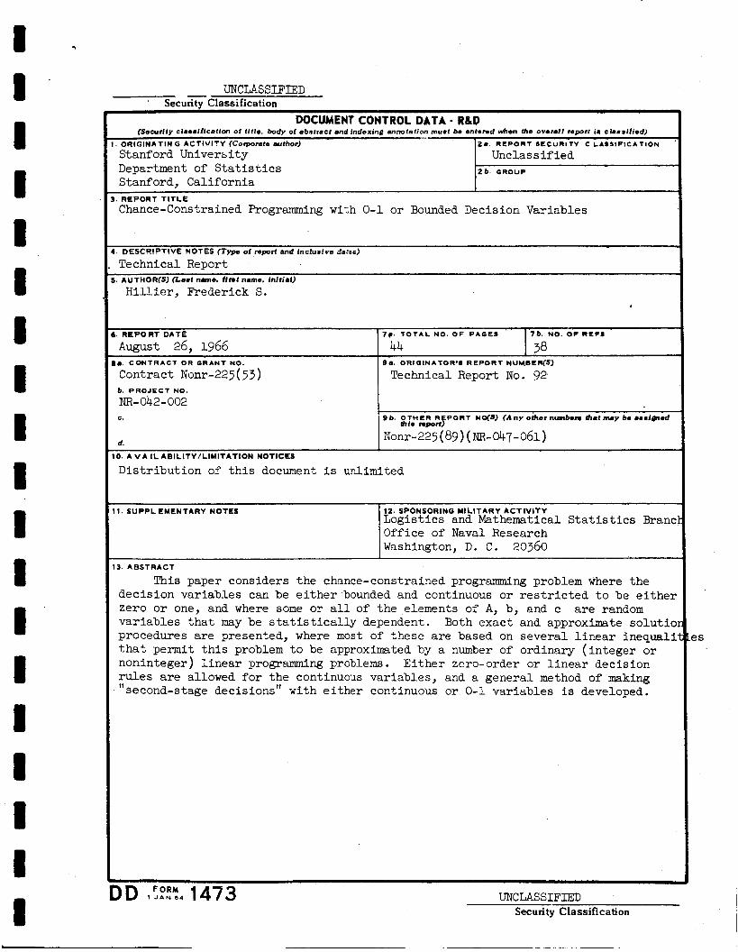
Chance-Constrained Programming with 0-1 or Bounded Decision Variables

Unclas s if ied

3 REPORT T I T L E

4 DESCS!PTIVE NOTES (Typo of report a i d ixclsaivs 6s:ss)

. Technical Report I AUTHOR(S) (Leet n m e . Hnt nuns. initial)

Hi l l i e r , Frederick S.

6. R E P 0 RT DATE 7p. T O T A L NO. OF PACES

August 26, 1966 44 76. NO. OF REFS

38 8.. C O N T R A C T OR GRANT NO.

Contract Konr-225( 53)

NR- 042- 002 b. P R O J E C T NO.

C .

d.

- 13. ABSTRACT

This paper considers the chance-constrained programming problem where the decision variables can be e i t h e r bounded and continuous o r r e s t r i c t e d t o be either zero or one, and where some or a l l of the elements of A, b, and c are random variables t h a t may be s t a t i s t i c a l l y dependent. Both exact and approximate so lu t ic procedures a re presented, where most of these a re based on several l i n e a r inequal1 t h a t permit t h i s problem t o be approximated by a number of ordinary ( in teger o r noninteger) l i nea r programming problems. Ei ther zero-order or l i n e a r decisior. rules are allowed f o r the continuous variables, and a general method of making "second-stage decisions" with e i ther continuous o r 0-1 variables i s developed.

98. ORIOINATOR'S R E P O R T yUWmLR(s)

Technical Report No. 92

Ob. O T H E R R P O R T YWS) (Any other nmborr h a t n u y be eeeigled hie rapor3

i~onr-225(89) (NR-047-061)

11. SUPPLEMENTARY NOTES

es

12. SPONSORING MILITARY ACTIVITY Logistics and Mathematical S t a t i s t i c s Branc Office of Naval Research Washington, D. C . 20360

v

UNCLASSIFIED Security Classification

14 K E Y WORDS

operat ions research mathematical programming chance-cons t ra ined programming l i n e a r programming under u n c e r t a i n t y l i n e a r bounds

~ ~~

INSTRUCTIONS 1. ORIGINATING ACTIVITY Enter the name and address of the contractor, subcontractor, grantee, Department of De- fense activity or other organization (corporate author) issuing t h e report.

243. REPORT SECUWTY CLASSIFICATION Enter the o v e r a l l security c lassi f icat ion of the report. Indicate whether “Restricted Data” is included Marking is to b e in a c c o r d ance with appropriate securi ty regulations.

2b. GROUP: Automatic downgrading i s specif ied in DoD Di- rect ive 5200.10 and Armed Forces Industrial Manual. Enter the group number. Also, when applicable. show that optional markings have been used for Group 3 and Group 4 a s author- ized.

3. REPORT TITLE. Enter the complete report t i t le in all capi ta l letters. T i t l e s in a l l cases should be unclassified. If a meaningful t i t le cannot be selected without c lass i f ica- tion, show t i t le c lass i f icat ion in all capi ta l s in parenthesis immediately following the title.

4. DESCRIPTIVE NOTES If appropriate, enter the type of report, e.g., interim, progress, summary, annual, or final. Give the inclusive da tes when a specif ic reporting period i s covered. 5. AUTHOR(S): Enter the name(s) of authods) a s shown on or in the report. If xilitary, show rank and branch of service. T h e name of t h e principal ,;ithor is an absolute minimum requirement 6. REPORT D A T Z Enter the date of the report a s day, month, year; or month, year. on the report, u s e d a t e of publ icat ion 743. TOTAL NUMBER OF PACES: T h e total page count shouid follow normal pagination procedures, Le., enter the number of pages containing information. 76. NUMBER O F REFERENCES Enter the total number of references ci ted in the report. 88. CONTRACT OR GRANT NUMBER: If appropriate, enter the applicable number of t h e contract or grant under which t h e report was written. 86, &, & 8d. PROJECT NUMBER. Enter the appropriate military department identification, such a s project number, subproject number, system numbers, task number, etc. 9a. ORIGINATOR’S REPORT NUMBER(S): Enter the offi- c ia l report number by which the document will be identified and controlled by t h e originating activily. b e unique to this report.

9b. OTHER REPORT NUMBER(S): If t h e report has been assigned any other report numbers (either b y the orrgiriator or by the sponsor), a lso enter ths number(s).

10. AVAILABILITY/LIMITATION NOTICES: Enter any lim- itations on further dissemination of the report, other than’thosi

Entei l a s t name, first name, middle initial.

If more than one date appears

This number must

- Lit

R O L E

1 LIP

R O L E W T

imposed by security c lassi f icat ion, using standard s ta tements such as:

(1)

(2)

(3)

“Qualified requesters may obtam copies of t h i s report from D D C ”

“Foreign announcement and dissemination of t h i s report by DDC is not au thor ized” “U. S. Government agencies may obtain copies of this report directly from DDC. Other qualified DDC users shal l request through

(4) “U. S. military agencies may obtain copies of th i s report directly fw-n DDC Other qualified u s e r s shal l request through

t ,

(5) “All distribution of this report i s controlled. Qual- ified DDC users shall request through

,#

If the report h a s been furnished tc the Office of Technical Services, Department of Commerce, for s a l e to the public, indi- c a t e t h i s fact and enter the price, if known. 11. SUPPLEMENTARY NOTES: U s e for additional explana- tory notes. 12. SPONSORING MILITARY ACTWITY Enter the name of the departmental project office or laboratory sponsoring (pay- ing for) the research and development. Include address. 13. ABSTRACT: Enter an abstract giving a brief and factual summary of the document indicative of the report, even though i t may a l so appear e lsewhere in the body of the technical re- port. If additional s p a c e i s required, a continuation s h e e t sha l l be attached.

It is highly desirable that the abstract of c lass i f ied reports be unclassified. Each paragraph of the abstract shal l end with an indication of the military security c lassi f icat ion of the in- formation in the paragraph, represented a s ITS). (S). IC). or (0).

There i s no limitation CII the length of the abstract. ever, the suggested length i s from 150 t9 225 words.

14. KEY WORDS: Key words are technically meaningful terms or short phrases that character ize a report and may be used a s index ent-ies for cataloging the report. se lected s o that n o security c lassi f icat ion i s required. Identi- fiers, such a s equipment model designation, trade name, militaq project code name. geographic location, may be used a s key words but wi!l be followed by an indication of technical con- text.

How-

Key words m u s t be

The assignment of l i n k s . rules, and weights is optional

GPO 8 8 6 - 5 5 1

TI Security Classification

c 8 1 I I 8 I I I I I I I I I 1 I I I 1