2502 Analysis

MT2502 Analysis

Mike Todd

19th November 2015

2

0.1 What is Analysis?

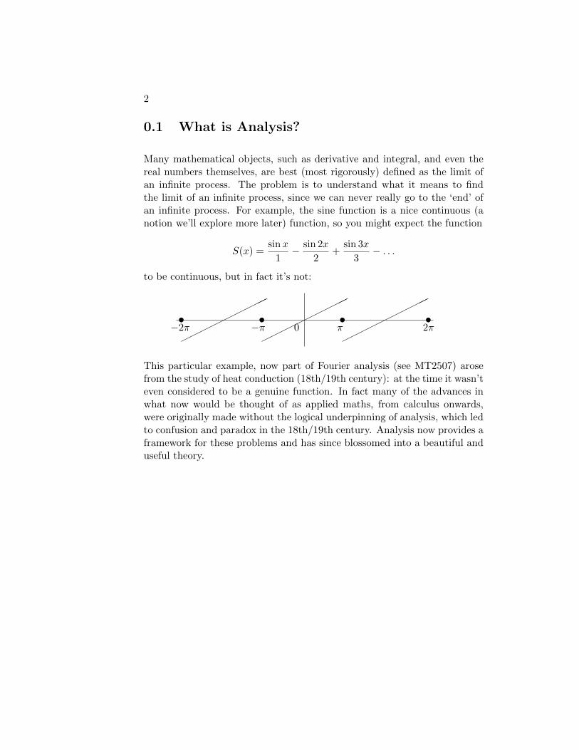
Many mathematical objects, such as derivative and integral, and even thereal numbers themselves, are best (most rigorously) defined as the limit ofan infinite process. The problem is to understand what it means to findthe limit of an infinite process, since we can never really go to the ‘end’ ofan infinite process. For example, the sine function is a nice continuous (anotion we’ll explore more later) function, so you might expect the function

S(x) =sinx

1− sin 2x

2+

sin 3x

3− . . .

to be continuous, but in fact it’s not:

��

��

��

��

��

��tt t t−π 0−2π π 2π

This particular example, now part of Fourier analysis (see MT2507) arosefrom the study of heat conduction (18th/19th century): at the time it wasn’teven considered to be a genuine function. In fact many of the advances inwhat now would be thought of as applied maths, from calculus onwards,were originally made without the logical underpinning of analysis, which ledto confusion and paradox in the 18th/19th century. Analysis now provides aframework for these problems and has since blossomed into a beautiful anduseful theory.

Chapter 1

The rationals and the reals

The real number system is a very intuitive idea and has been used sinceat least the ancient Greek times. However, while ostensibly higher-powerednotions like derivative and integral (1820s) use this intuitive notion, a rigor-ous formal definition of the real numbers came much later (1860s-early 20thcentury).

In this section, we’ll discuss the construction of the reals using precise defin-itions, logic, set theory and the rational number system (although we’ll haveto leave out some of the construction in the interests of time).

First recall that the set of rational numbers Q is defined as the collection ofall fractions of the form p

q where p ∈ Z and q ∈ N.

The first result is that adding/subtracting/multiplying two rational numbersyields a rational number: Q is closed under the usual algebraic operations.

Proposition 1.1. If a, b ∈ Q, then a+ b, a− b, ab ∈ Q. Moreover, if b 6= 0then a

b ∈ Q.

The proof is an exercise.

While the rationals are a nice set from many points of view, they are insuf-ficient for even the most basic mathematics. Eg a right-angled triangle withsides of length 1 and 1, by Pythagoras’ Theorem has hypotenuse of length√

2. But√

2, which by definition is the positive solution x to x2 = 2, isn’trational:

3

4 CHAPTER 1. THE RATIONALS AND THE REALS

Proposition 1.2. There is no rational number x such that x2 = 2.

Proof. Suppose that, on the contrary, there is some x = pq where p, q ∈ N

such that x2 = 2. First notice that if p and q have a common divisor (aninteger which divides both) then we can factorise this out. Hence w.m.a. pand q have no common divisors.

Since x2 = 2,

p2

q2= 2⇒ p2 = 2q2, (1.0.1)

we know that p must be even (note that the only way a square of a numbercan be even is if the number itself is even). So p is even, so there mustexist n ∈ N such that p = 2n. Hence p2 = (2n)2 = 2q2 ⇒ 2n2 = q2, sosimilarly q is even. So p and q have a common divisor of 2, contradictingour assumption. Hence the proposition must be true.

This proposition implies that there are ‘holes’ in the rational numbers. In thesame vein, the following example shows that while you can take a sequenceof rational numbers which intuitively converge, they need not converge to arational number.

Example 1.1. Let x1 = 2 and for n > 1, let

xn+1 =xn2

+1

xn

(i.e., x1 = 2, x2 = 22 + 1

2 = 32 , x3 =

( 32)2 + 1

( 32)

= 34 + 2

3 = 1712 .)

Claim. The sequence is decreasing, i.e., x1 > x2 > x3 > · · · .

Proof. We’ll show that xn − xn+1 > 0 for any n.

1.1. ORDERING AND BOUNDING 5

First, since x1 = 2 > 32 = x2, the claim is proved for n = 1. For n > 2:

xn − xn+1 = xn −(xn2

+1

xn

)=xn2− 1

xn=

1

2xn(x2n − 2)

=1

2xn

((xn−1

2+

1

xn−1

)2

− 2

)=

1

2xn

(x2n−1

4+ 1 +

1

x2n−1− 2

)=

1

2xn

(x4n−1 + 4− 4x2n−1

4x2n−1

)=

1

2xn

((x2n−1 − 2)2

4x2n−1

)> 0.

The sequence is also bounded:

0 6 xn 6 x1 = 2 ∀n ∈ N.

Suppose now that, contrary to the statement of the proposition, (xn)n doesconverge to a number x ∈ Q. But since xn+1 = xn

2 + 1xn

, any such limitmust satisfy

x =x

2+

1

x⇒ x

2=

1

x⇒ x2 = 2,

which by Proposition 1.2 is impossible if x ∈ Q.

It is strange that a bounded decreasing sequence in Q doesn’t converge inQ. For such reasons we need to extend our set of numbers.

1.1 Ordering and bounding

Before defining the reals, we’ll need some abstract, but widely applicable,definitions.

Definition 1.1. An ordered set (X,<) consists of a set X and a relation< on X such that

1. The trichotomy law holds: exactly one of the following is true:

x < y, x = y, y < x.


2. The transitivity law holds: if x, y, z ∈ X and x < y and y < z thenx < z.

We’ll also use the notation x 6 y which means that x < y or x = y; x > y,which means y < x; and x > y which means y 6 x.

Ordered sets can be very abstract, but a fairly concrete example is (Q, <),i.e., the rational numbers with the usual ordering <.

Definition 1.2. Given an ordered set (X,<) and A ⊆ X,

1. u ∈ X is called an upper bound for A if

∀a ∈ A, a 6 u.

If there is an upper bound, we say that A is bounded above

2. ` ∈ X is called an lower bound for A if

∀a ∈ A, ` 6 a.

If there is a lower bound, we say that A is bounded below.

If A is bounded both above and below, we say that A is bounded.

N.B. There may be lots of upper/lower bounds for given sets A, whichcontrasts with the following notions.

Definition 1.3. Let (X,<) be an ordered set and A ⊆ X.

1. An element M ∈ A is called a maximum for A if M is an upper boundfor A, i.e., we require

∀a ∈ A, a 6M and M ∈ A.

2. An element m ∈ A is called a minimum for A if m is an lower boundfor A, i.e., we require

∀a ∈ A, m 6 a and m ∈ A.

1.1. ORDERING AND BOUNDING 7

Note that there can be at most one maximum for A: suppose we had two,say M1 and M2. Then by definition,

M2 6M1 and M1 6M2, so M1 = M2.

Similarly, there’s at most one minimum.

Assuming it exists, we denote the unique maximum by

maxA, maxx∈A

x, or max{x ∈ A},

and similarly the unique minimum by

minA, minx∈A

x, or min{x ∈ A}.

Problem: Maxima/minima may not exist. Eg, set

I := {q ∈ Q : 0 < q 6 1}.

This set is bounded above (eg by 70) and below (eg by 0), but while it hasa maximum (i.e., 1), it has no minimum. To cope with this kind of issue,define:

Definition 1.4. Let (X,<) be an ordered set and A ⊆ X a non-emptysubset of X.

1. Let U(A) denote the set of upper bounds for A. Then an elementu ∈ U(A) is called a least upper bound/supremum for A if

∀v ∈ U(A), u 6 v.

2. Let L(A) denote the set of lower bounds for A. Then an element` ∈ L(A) is called a greatest lower bound/infimum for A if

∀m ∈ L(A), m 6 `.

There can be at most one supremum (Exercise), so we denote this, if itexists, by

supA, supx∈A

x, sup{x ∈ A}.

Similarly for infimum,

inf A, infx∈A

x, inf{x ∈ A}.


Lemma 1.3. For A a non-empty subset of Q:

1. if A has a maximum, then maxA = supA;

2. if A has a minimum, then minA = inf A.

Proof. See tutorial sheet.

Example 1.2. Recall the set I := {x ∈ Q : 0 < x 6 1}. Since I has amaximum, 1, then it shares the same supremum. However, while it doesn’thave a minimum, inf I = 0 (first 0 is clearly a lower bound; suppose that` > 0 is an infimum: then for large enough n, 1

n < `, so since 1n ∈ I, ` isn’t

a lower bound for I).

Example 1.3. Given the ordered set (Q, <), define

K := {q ∈ Q : 0 < q, q2 < 2}.

Clearly this set is bounded. However,

Proposition 1.4. K has no supremum.

Proof. Suppose that the proposition is false, so there exists a least upperbound x ∈ Q for K. We’ll show that this is impossible.

Claim. 2 < x2.

Proof of claim. Suppose that the claim is false, so x2 6 2. Since x ∈ Q,Proposition 1.2 implies that x2 6= 2, so in fact x2 < 2. Therefore, 2−x2

2x+1 > 0.

So choosing n ∈ N large enough, we can ensure that 2−x22x+1 >

1n (*). Then(

x+1

n

)2

= x2 +2x

n+

1

n2= x2 +

1

n

(2x+

1

n

)6 x2 +

1

n(2x+ 1) < x2 + (2− x2) (by (*))

= 2

So x + 1n is a rational number whose square is < 2 and hence in K, so x

can’t be an upper bound on K, a contradiction.

1.2. ABSOLUTE VALUE 9

The claim implies that x2 > 2, so x2−22x > 0 and so we can choose m ∈ N so

that x2−22x > 1

m , which rearranges to

x2 − 2x

m> 2 (**).

Set y := x− 1m < x. Then

y2 = x2 − 2x

m+

1

m2> x2 − 2x

m> 2

by (**). Hence y < x is an upper bound for K, contradicting x being a leastupper bound.

Adding this all together, the proposition is true.

We want to work in a set of numbers which has no such ‘holes’, i.e., allbounded subsets have supremum/infimum.

Definition 1.5. An ordered set (X,<) is called complete if every non-emptyset which is bounded above has a supremum.

Note that (Q, <) is not complete by Proposition 1.4.

In the following result we’ll use the notion of ‘field’ see eg Section 1.4 ofHowie.

Theorem 1.5. There exists an ordered field denoted (R, <) such that

i) Q ⊆ R

ii) (R, <) is complete.

We omit the proof of this theorem, as well as the theorem which states that(R, <) is essentially unique.

The set above is called the real numbers R. Note that elements of R \Q arecalled irrational numbers.

1.2 Absolute Value

(Note that this short section doesn’t particularly fit into this chapter, butit’ll be useful later.)


Definition 1.6. Given x ∈ R, the absolute value of x, denoted |x|, is definedas

|x| :=

{−x if x < 0,

x if x > 0.

Theorem 1.6. Given x, y ∈ R and a > 0,

i) |x| > 0;

ii) | − x| = |x|;

iii) |x| 6 a iff −a 6 x 6 a;

iv) |xy| = |x||y|;

v) (Triangle inequality) |x+ y| 6 |x|+ |y|;

vi) (Reverse triangle inequality)∣∣∣|x| − |y|∣∣∣ 6 |x− y|.

Proof. i)-iv): Exercise.

v): Since −|x| 6 x 6 |x| and −|y| 6 y 6 |y|, summing:

−(|x|+ |y|) 6 x+ y 6 |x|+ |y|,

so applying iii), we obtain v).

vi) Exercise.

N.B. Absolute value is often used as a way of finding the distance betweentwo real numbers x, y ∈ R: i.e., this is |x− y|.

Chapter 2

Sequences

Now that we’ve laid a solid foundation for the real number system we canbegin to address more ‘analytic’ issues; the first of these being sequences.

2.1 Sequences and convergence

Definition 2.1. A sequence of real numbers is a function

f : N→ R

going from the rationals to the reals. Usually we’ll denote f(n) by xn andwrite the sequence as

(xn)n, (xn)n∈N, (xn)∞n=1, (x1, x2, . . .).

Note that in contrast to set notation { }, the order is important here, eg(−1, 1, 1,−1, . . .) means something different to {−1, 1, 1,−1, . . .} = {−1, 1}.Moreover, (1, 2, 3, 4, 5, . . .) 6= (2, 1, 3, 4, 5, . . .).

Sometimes we have a nice formula for the n-th term of a sequence, eg

(2, 4, 6, 8, . . .) = (2n)n i.e., xn = 2n;

(1,

1

2,1

3,1

4, . . .

)=

(1

n

)n

i.e., yn =1

n.

Example 2.1. • If b ∈ R then the sequence (xn) = (b, b, b, . . .) is calledthe constant sequence b. Eg the constant sequence 300 is (300, 300, 300, 300, . . .).

11

12 CHAPTER 2. SEQUENCES

• Given the expression xn = (−1)n for n ∈ N, we obtain

(xn)n = (−1, 1,−1, 1, . . .).

• For an = (−1)n2n for n ∈ N, we obtain (an) =

(−12 ,

14 ,−18 , . . .

).

Definition 2.2. Let (xn)n be a sequence of real numbers and x ∈ R.

1. We say that (xn)n converges to x (as n tends to infinity) if

∀ε > 0 ∃N ∈ N s.t. ∀n ∈ N, n > N ⇒ |xn − x| 6 ε.

In this case we write

limnxn = x, lim

n→∞xn = x, xn → x as n→∞

A sequence (xn)n is called convergent if there exists x ∈ R such thatlimx→∞ xn = x; otherwise the sequence is called divergent.

2. We say that (xn)n tends to infinity (as n tends to infinity) if

∀K ∈ R ∃N ∈ N s.t. ∀n ∈ N, n > N ⇒ xn > K.

In this case we write

limnxn =∞, lim

n→∞xn =∞, xn →∞ as n→∞

3. We say that (xn)n tends to minus infinity (as n tends to infinity) if

∀K ∈ R ∃N ∈ N s.t. ∀n ∈ N, n > N ⇒ xn 6 K.

limnxn = −∞, lim

n→∞xn = −∞, xn → −∞ as n→∞

In other words, if xn → x then no matter how small ε > 0 is chosen, therewill be some stage in the sequence (stage N) beyond which all elements xnwill lie in the interval [x− ε, x+ ε].

Example 2.2.(

1n2

)n

is convergent:

Proof. Let ε > 0. Given N ∈ N, if n > N then∣∣∣∣ 1

n2− 0

∣∣∣∣ =1

n26

1

N2.

So choosing N so that 1N2 < ε, i.e., N > 1√

εcompletes the proof.

2.1. SEQUENCES AND CONVERGENCE 13

Example 2.3. Let x be some real number and let (xn)n be the constantsequence (x, x, x, . . .). Then

xn → x as n→∞.

Proof. Let ε > 0. Then given N ∈ N, n > N implies

|xn − x| = |x− x| = 0 6 ε,

as required.

Example 2.4. The sequence(1n

)n

converges to 0 as n→∞.

Proof. Let ε > 0. Fix N ∈ N such that N > 1ε . Then

|xn − 0| =∣∣∣∣ 1n − 0

∣∣∣∣ =1

n6

1

N6 ε,

as required.

Example 2.5. The sequence(4n+3005n+2

)n

is convergent: in fact

4n+ 300

5n+ 2→ 4

5as n→∞.

Proof. Let ε > 0. For N ∈ N, n > N implies∣∣∣∣4n+ 300

5n+ 2− 4

5

∣∣∣∣ =

∣∣∣∣5(4n+ 300)− 4(5n+ 2)

5(5n+ 2)

∣∣∣∣ =1492

25n+ 10<

1492

25N.

So setting N > 149225ε , we complete the proof.

Example 2.6. For xn = (−1)n, the sequence (xn)n is divergent.

(Idea: suppose there is a limit x and then show that there is some ε > 0 forwhich |xn − x| > ε even for some very large n.)

Proof. Suppose that there is a limit, call it x ∈ R. Then set ε = 12 . Since x

is a limit, there exists N such that n > N implies |xn − x| 6 12 . Since there

are arbitrarily large even numbers, there is always some n > N (eg n = 2N)such that xn = 1, so |1 − x| 6 1

2 , in particular, x > 12 . On the other hand,

since there are arbitrarily large odd numbers, there is always some n > N(eg n = 2N + 1) such that xn = −1, so | − 1− x| 6 1

2 , hence x 6 −12 . The

inequality 12 6 x 6 −1

2 is impossible, so there is no limit.


Example 2.7. (√n)n tends to ∞ as n→∞.

Proof. Let K > 0. Then set N ∈ N to be greater than K2. Hence n > Nimplies xn =

√n >√N > K, as required.

Example 2.8.(1n − n

)n

tends to −∞ as n→∞.

Proof. Let K ∈ R. Then set N ∈ N so that N > 1−K. So n > N implies

xn =1

n− n 6 1−N < K,

as required.

Example 2.9. (Standard sequences) Let a ∈ R.

1. If |a| < 1 then (an)n converges to 0.

2. If a > 1 then (an)n tends to ∞.

Proof. We assume Bernoulli’s Inequality: for x > 0 and n ∈ N,

(1 + x)n > 1 + nx (∗).

(Proof is an easy exercise in induction.)

1) Using the fact that |a| < 1 to deduce that 1|a| − 1 > 0, for N ∈ N and

n > N ,

|an−0| = |a|n =1(

1 +(

1|a| − 1

))n 61(

1 + n(

1|a| − 1

)) 61(

1 +N(

1|a| − 1

)) ,so choosing N ∈ N such that N > 1

ε(

1|a|−1

) , we are finished.

2) Let K ∈ R. Then for n ∈ N and n > N ,

an = (1 + (a− 1))n > 1 + n(a− 1) > N(a− 1).

So if N > Ka−1 , we are finished.

2.2. LIMIT THEOREMS 15

2.2 Limit Theorems

In this section we’ll consider uniqueness and algebraic properties of limits.

Theorem 2.1. If a sequence is convergent, its limit is unique.

Proof. Let (xn)n be a sequence that converges to both s and t. Let ε > 0.Then since xn → s, there exists N1 ∈ N such that n > N1 implies

|xn − s| 6 ε.

Similarly, since xn → t, there exists N2 ∈ N such that n > N2 implies

|xn − t| 6 ε.

Therefore taking n > max{N1, N2},

|s− t| = |s− xn + xn − t| 6 |s− xn|+ |xn − t| 6 ε+ ε = 2ε.

Since this holds for any ε > 0, this means s = t.

If a sequence can have very large values for large n, this can cause problemsfor the algebraic properties of that sequence (eg see next theorem). Thefollowing definition deals with that.

Definition 2.3. A sequence (xn)n is called bounded if there exists M > 0such that |xn| 6M for all n ∈ N.

Theorem 2.2. Every convergent sequence is bounded.

Proof. Suppose that (xn)n is a convergent sequence and denote its limit byx ∈ R. Then there exists N ∈ N such that |xn − x| 6 1 for all n > N . Son > N implies

|xn| = |xn − x+ x| 6 |xn − x|+ |x|.

So definingM := max {|x1|, |x2|, . . . , |xN |, |x|+ 1}, we deduce that |xn| 6Mfor all n ∈ N.

The next theorem simplifies many questions involving combinations of morethan one sequence.


Theorem 2.3. Let a ∈ R and (xn)n, (yn)n be convergent sequences withxn → x and yn → y as n→∞. Then

1. xn + yn → x+ y;

2. xnyn → xy;

3. If yn 6= 0 for all n ∈ N and y 6= 0 then 1yn→ 1

y ;

4. If yn 6= 0 for all n ∈ N and y 6= 0 then xnyn→ x

y ;

5. axn → ax and a+ xn → a+ x.

Proof. 1) Let ε > 0. Since xn → x, there exists N1 ∈ N such that

|xn − x| 6ε

2∀n > N1.

Similarly, since yn → y, there exists N2 ∈ N such that

|yn − y| 6ε

2∀n > N2.

Set N := max{N1, N2}. Then n > N implies

|(xn + yn)− (x+ y)| = |(xn − x) + (yn − y)| 6 |xn−x|+|yn−y| 6ε

2+ε

2= ε,

as required.

2) Let ε > 0. First note that

|xnyn − xy| = |xnyn − xny + xny − xy|6 |xnyn − xny|+ |xny − xy|6 |xn||yn − y|+ |y||xn − x| (∗)

Since xn → x, there exists N1 ∈ N such that |xn − x| 6 ε2(|y|+1) for all

n > N1.

By Theorem 2.2, (xn)n is bounded, i.e., there exists M > 0 such that |xn| 6M for all n ∈ N . Since also yn → y, there exists N2 ∈ N such that|yn − y| 6 ε

2(M+1) for all n > N2. Let N := max{N1, N2}. Then by (∗),n > N implies

|xnyn−xy| 6 |xn||yn− y|+ |y||xn−x| 6M · ε

2(M + 1)+ |y| · ε

2(|y|+ 1)6 ε,

2.2. LIMIT THEOREMS 17

as required.

3) Let ε > 0. First observe that∣∣∣∣ 1

yn− 1

y

∣∣∣∣ =

∣∣∣∣y − ynyny

∣∣∣∣ =|y − yn||y||yn|

(∗∗).

Since yn → y, there exists N1 ∈ N such that n > N1 implies

|y − yn| 6|y|2∀n > N1.

Therefore,

|y| = |yn + (y − yn)| 6 |yn|+ |y − yn| 6 |yn|+|y|2

which implies |yn| > |y|2 for all n > N1.

Moreover, there exists N2 ∈ N such that n > N2implies

|yn − y| 6ε|y|2

2∀n > N2.

So setting N := max{N1, N2}, (∗∗) implies∣∣∣∣ 1

yn− 1

y

∣∣∣∣ 6 ε|y|2

2|y|(|y|2

) = ε,

as required.

4) Since xnyn

= xn · 1yn

, this follows by 2) and 3).

5) Exercise.

Example 2.10. Let p ∈ N. Then (xn)n =(2 + 1

np

)n

converges to 2.

Proof. Let (an)n be the constant sequence 2 and let (bn)n be the sequencegiven by bn = 1

np for all n ∈ N. Then xn = an + bn.

Further, let cn = 1n for all n ∈ N. We know that 1

n → 0 as n → ∞. So byTheorem 2.3, cncn · · · cn = cpn → 0 as n→∞. Hence an → 2 and bn → 0 asn→∞, so by Theorem 2.3, xn → 2 + 0 = 2 as n→∞.


(Above we used the constant sequence 2 and the sequence (1/n)n as buildingblocks for which we knew the limiting behaviour. We’ll be able to use thistype of idea from here on, unless we are asked to prove ‘from first principles’(or a similar phrase) that a sequence converges.)

Example 2.11. The sequence(n2+4nn3−3

)n

is convergent, in fact

(n2 + 4n

n3 − 3

)n

→ 0 as n→∞.

Proof.

n2 + 4n

n3 − 3=

1n + 4

n2

1− 3n3

=1n + 4

(1n

)21− 3

(1n

)3 .Since 1

n → 0, by Theorem 2.3,

n2 + 4n

n3 − 3=

1n + 4

(1n

)21− 3

(1n

)3 → 0 + 4 · 02

1− 3 · 03= 0.

2.3 Monotone Sequences and Subsequences

In most of our examples of convergent sequences so far, proving convergencehas involved guessing a limit before taking any further steps. In this sectionwe’ll develop tools which can overcome this problem: even when we don’thave a candidate for a limit, in some cases we can use the completeness ofthe reals to guarantee that one exists.

Definition 2.4. Let (xn)n be a sequence of real numbers.

• We say that a sequence is increasing if it satisfies x1 6 x2 6 x3 6 · · · .

• We say that a sequence is decreasing if it satisfies x1 > x2 > x3 > · · · .

• We say that a sequence is monotone if it is either increasing or de-creasing.

Example 2.12. a) (an) = (n)n is increasing;

2.3. MONOTONE SEQUENCES AND SUBSEQUENCES 19

b) (bn) = (4n)n is increasing;

c) (cn) =(3− 1

n

)n

is increasing;

d) (dn) = (1, 1, 2, 2, 3, 3, 4, 4, . . .)n is increasing (despite some adjacentterms being equal);

e) (en) =(3n

)n

is decreasing;

f) (fn) = (−2n)n is decreasing;

g) (gn) = (k, k, k, k, . . .) for some k ∈ R is both increasing and decreasing;

h) (hn) = ((−1)n)n is not monotone;

i) (in) =((−1)nn

)n

is not monotone.

Note that (cn)n, (en)n, (gn)n, (hn)n, (in)n are all bounded, while (an)n, (bn)n, (dn)nare unbounded. Also note that the bounded monotone sequences ((cn)n, (en)n, (gn)n)are convergent, while the unbounded sequences are not (as in Theorem 2.2).These are examples of a broader phenomenon:

Theorem 2.4 (Monotone Convergence Theorem). Let (xn)n be a monotonesequence. Then the following are equivalent:

1. (xn)n is convergent;

2. (xn)n is bounded.

Proof. (1⇒ 2): This is true by Theorem 2.2.

(2⇒ 1): Assume first that (xn)n is bounded and increasing. Let A := {xn :n ∈ N}. Since we have assumed that A is bounded, A has a supremumx = supA ∈ R by the completeness of the reals.

Claim. xn → x as n→∞.

Proof of Claim. Let ε > 0. Since x = supA, x − ε is not an upper boundfor A. Hence there exists N ∈ N such that xN > x − ε. Since (xn)n isincreasing, n > N implies

x− ε 6 xN 6 xn 6 x, i.e., |xn − x| 6 ε ∀n > N,

so the claim is proved.


The proof where (xn)n is decreasing is similar.

Corollary 2.5. Suppose that (xn)n is a bounded sequence.

1. If (xn)n is increasing then limn→∞ xn = supn xn.

2. If (xn)n is decreasing then limn→∞ xn = infn xn.

Proof. This follows immediately from the proof of Theorem 2.4.

Example 2.13. If 0 < a < 1 then an → 0 as n → ∞. (Note that we’vealready proved this, but here’s an alternative proof.)

Proof. Let xn = an. Since an+1 < an for all n ∈ N, (xn)n is a decreasingsequence bounded above by a and below by 0. So MCT implies there is alimit x ∈ R. Therefore (see eg TS2 Q11) xn+1 → x also. So xn+1 = an+1 =axn → x. But since xn → x, Theorem 2.3 implies that axn → ax. Henceax = x. Since a 6= 1, the only solution is x = 0.

Exercise: extend this to |a| < 1.

Example 2.14. Define (xn)n by x1 = 1 and xn+1 =√

1 + xn for n ∈ N.The sequence is bounded and increasing, thus convergent: indeed

xn →1 +√

5

2.

Proof. Claim 1. |xn| 6 2 for all n ∈ N.

Proof of Claim 1. We prove this by induction. For n = 1, x1 = 1 6 2.Suppose that the claim is true for n ∈ N. Then

xn+1 =√

1 + xn 6√

1 + 2 =√

3 6 2,

so the claim is true for n+ 1. Hence by induction, the claim holds.

Claim 2. (xn)n is increasing, i.e., for all n ∈ N, xn 6 xn+1.

Proof. For n = 1 we have x1 = 1 6√

1 + 1 = x2. Assume the claim is truefor n ∈ N. Then xn+1 =

√1 + xn 6

√1 + xn+1 = xn+2, so the claim is true

for n+ 1. Hence by induction the claim holds.


Combining these claims and the MCT there exists x ∈ R such that xn → x.

By Theorem 2.3, 1 + xn → 1 + x, and by TS2 Q5, setting yn = 1 + xn andy = 1 + x, we have

√yn →

√y, i.e.,

√1 + xn →

√1 + x. Since xn+1 =√

1 + xn → x, this means that x =√

1 + x and hence x2 = 1 +x. Therefore

x =1 +√

5

2or x =

1−√

5

2.

But since xn > 0 for all n ∈ N, only the positive solution for x is possible,

i.e., x = 1+√5

2 .

Example 2.15. Let (xn)n be given by

xn =1

12+

1

22+

1

32+ · · ·+ 1

n2.

The sequence is bounded and increasing, and hence convergent (in fact the

limit is π2

6 , but we won’t show that here).

Proof.

Claim. 0 < xn 6 2 for all n ∈ N.

Proof of Claim. We write

0 61

12+

1

22+

1

32+

1

42+ · · ·+ 1

n26 1 +

1

1 · 2+

1

2 · 3+

1

3 · 4+ · · ·+ 1

(n− 1)n

= 1 +

(1

1− 1

2

)+

(1

2− 1

3

)+

(1

3− 1

4

)+ · · ·+

(1

n− 1− 1

n

)= 1 + 1− 1

n6 2.

So (xn)n is bounded. Clearly (xn)n is increasing since

xn =1

12+

1

22+

1

32+ · · ·+ 1

n26

1

12+

1

22+

1

32+ · · ·+ 1

n2+

1

(n+ 1)2= xn+1,

so the proof is complete.

Definition 2.5. Let (xn)n be a sequence and (mk)k be a sequence of nat-ural numbers m1 < m2 < m3 < · · · . then the sequence (xmk)k is called asubsequence of (xn)n.


Note that in this definition, we must have mk > k for all k ∈ N.

Example 2.16. The sequence (xn)n =(1n

)n

has various subsequences, eg

• (sk)k = (x2k)k =(

12k

)k

=(12 ,

14 ,

16 , . . .

);

• (tk)k = (xk+3)k =(14 ,

15 ,

16 , . . .

);

• the sequence (xn)n is a subsequence of itself.

Note that eg(13 ,

12 ,

14 ,

15 ,

16 , . . .

)is not a subsequence of (xn)n: the order of

terms must be preserved.

Theorem 2.6. Suppose that (xn)n converges to x ∈ R. Then any sub-sequence also converges to x ∈ R.

Proof. Let ε > 0. Since xn → x then there exists N ∈ N such that n > Nimplies |xn − x| 6 ε. Since (xmk)k is a subsequence of (xn)n. Let K ∈ N besuch that k > N implies mk > N . Then

|xmk − x| 6 ε for all k > K,

as required.

N.B. that we could have made the statement of the theorem into an ‘if andonly if’ since if any subsequence of (xn)n converges to x, then certainly (xn)nconverges to x - since (xn)n is a subsequence of itself.

Theorem 2.7 (Monotone Subsequence Theorem). Any sequence of realnumbers (xn)n has a monotone subsequence.

Proof. In this proof, we say that p ∈ N is a ‘peak’ if

xp > xn for all n > p.

Case 1: (xn)n has infinitely many peaks. We list the peaks in the orderin which they occur: p1 < p2 < p3 < · · · . From the definition of peaks, wehave

xp1 > xp2 > xp3 > · · · ,

so (xpk)k is the monotone (decreasing) subsequence we require.


Case 2: (xn)n has finitely many peaks. Again we list all the peaks inthe order in which they occur: p1 < p2 < · · · < pN . Let t1 > pN . Sincet1 is not a peak, there exists t2 > t1 such that xt2 > xt1 . Since t2 isalso not a peak, there exists t3 > t2 such that xt3 > xt2 . Proceeding inthis way, we obtain an infinite sequence t1 < t2 < t3 < t4 < · · · suchthat xt1 < xt2 < xt3 < xt4 < · · · . So (xtk)k is the monotone (increasing)subsequence we require.

Theorem 2.8 (Bolzano-Weierstrass Theorem). Let (xn)n be a bounded se-quence of real numbers. Then there exists a subsequence (xmk)k and a realnumber x such that xmk → x as n→∞.

Proof. The Monotone Subsequence Theorem guarantees the existence of amonotone subsequence (xmk)k. Then since (xmk)k is also bounded, theMonotone Convergence Theorem implies that (xmk)k converges to some limitx.

Example 2.17. Let (xn)n = ((−1)n)n. Then this is a bounded sequence, egbounded above by 2 and below by −2. So the Bolzano-Weierstrass Theoremimplies there exists a convergent subsequence. In fact in this case we cancheck this by hand: eg the subsequence (x4n)n = (1, 1, 1, . . .) converges to 1.On the other hand, the subsequence (x6n+1)n = (−1,−1,−1, . . .) convergesto −1.

Example 2.18. Consider (sinn)n. Note that this sequence is bounded aboveby 1 and below by −1. Hence the Bolzano-Weierstrass Theorem implies thatthere exists (mk)k such that (xmk)k is a convergent subsequence. (In fact,while we won’t show this here, for any x ∈ [−1, 1] there exists a subsequencewhich converges to x.)

Chapter 3

Series

Outside maths, ‘sequence’ and ‘series’ are often understood to mean thesame thing. However, in maths they are distinct notions.

Notation: Given a sequence (xn)n, for n ∈ Z and m ∈ N with n 6 m, wewrite

xn + xn+1 + xn+2 + · · ·+ xm =m∑k=n

xk.

Definition 3.1. • Given a sequence (xn)n, we can formally writex1+x2+x3+· · · as

∑∞k=1. This is called the (infinite) series generated

by (xn)n.

• For each n ∈ N, we write

sn = x1 + x2 + · · ·+ xn =n∑k=1

xk,

the nth partial sum of our series.

• We say that the series∑∞

n=1 xn converges if the partial sums converge,i.e., the limit limn→∞ sn exists. In this case,

∑∞n=1 xn is the (infinite)

sum of our sequence (xn)n.

• If (sn)n does not converge, we say that the series diverges. If sn → +∞or sn → −∞, we write

∑∞n=1 xn = +∞,

∑∞n=1 xn = +∞ respectively.

N.B. If (sn)n doesn’t converge or tend to +∞ or −∞, then we don’t thinkof∑∞

n=1 xn as a sum.

25

26 CHAPTER 3. SERIES

Example 3.1. Consider the sequence (xn)n where xn = 1n(n+1) for all n ∈

N. The associated series is

∞∑n=1

xn =∞∑n=1

1

n(n+ 1).

The nth partial sum is

sn =n∑k=1

1

k(k + 1)=

1

1 · 2+

1

2 · 3+

1

3 · 4+ · · ·+ 1

n(n+ 1)

=

(1

1− 1

2

)+

(1

2− 1

3

)+

(1

3− 1

4

)+ · · ·+

(1

n− 1

n+ 1

)= 1− 1

n+ 1.

Since(

1n+1

)n

converges to 0 and (1)n converges to 1, then (sn)n =(

1− 1n+1

)n

converges to 1. Hence∑∞

n=1 xn is a convergent series with sum equal to 1.

Example 3.2. Let (xn)n = ((−1)n)n. Then the series this generates is∑∞n=1(−1)n. Here the nth partial sum is

sn =n∑k=1

(−1)k =

{−1 if n is odd,

0 if n is even.

Hence (sn)n is a divergent sequence (check), so (xn)n = ((−1)n)n is diver-gent.

In the first example, but not the second, the sequence which generatedthe sequence converged to zero. In fact this is necessary for a sequence toconverge:

Theorem 3.1. Let∑∞

n=1 xn be a convergent series. Then xn → 0 as n →∞.

Proof.∑∞

n=1 xn being convergent means that the partial sums (sn)n con-verge to some limit s. Note that

xn = sn − sn−1 for all n > 2.

Since sn → s and sn−1 → s, this means that xn → s−s = 0, as required.

27

It might be nice if the converse of this theorem were true (i.e., xn → 0 implies∑∞n=1 xn converges), but as in the next example, this isn’t true, which leads

to some fundamentally important theory.

Example 3.3. The harmonic series is defined as

∞∑n=1

1

n= 1 +

1

2+

1

3+ · · · .

Theorem 3.2.∑∞

n=11n =∞.

Proof. Letting sn =∑∞

k=11k be the nth partial sum, we’ll show sn →∞ by

grouping summands in an appropriate way. For k ∈ N, we write

s2k = 1 +

(1

2

)+

(1

3+

1

4

)+

(1

5+

1

6+

1

7+

1

8

)+

(1

9+

1

10+

1

11+ · · ·+ 1

16

)+ · · ·+

(1

2k−1 + 1+

1

2k−1 + 2+ · · ·+ 1

2k

).

So the jth bracketed expression is

tj =1

2j−1 + 1+

1

2j−1 + 2+ · · ·+ 1

2j.

There are 2j − 2j−1 = 2j−1(2− 1) = 2j−1 terms in this sum, each of whichis > 1

2j. So tj > 2j−1 1

2j= 1

2 for any j ∈ N. Hence

s2k = 1 + t1 + t2 + · · ·+ tk > 1 +k

2.

So for any M ∈ R, let M ′ >M be an integer. Then n > 22M′

implies that

sn > s22M′ > 1 +2M ′

2= 1 +M ′ > M.

So sn →∞, as required.

Example 3.4. Given a ∈ R and r ∈ R\{0}, the sequence (arn−1)n generatesthe geometric series

∑∞n=1 ar

n−1.

Theorem 3.3. The geometric series∑∞

n=1 arn−1 converges if and only if

|r| < 1. When |r| < 1 then∑∞

n=1 arn−1 = a

1−r .


Proof. We start by noting that the nth partial sum is

sn = a+ ar + ar2 + · · ·+ arn−1 =a(1− rn)

1− r(Exercise).

So if |r| < 1 then rn → 0 (see Example 2.9), so sn → a1−r by Theorem 2.3.

If r = 1 then sn = na which tends to +∞ if a > 0 and −∞ if a < 0.

If r = −1, then sn is zero if n is even and a if n is odd, so the series isdivergent.

If |r| > 1 then (sn)n diverges (Exercise).

So a particular case is the sequence((

12

)n−1)n

generating the series

∞∑n=1

(1

2

)n−1= 1 +

1

2+

1

4+

1

8+ · · · = 1

1− 12

= 2.

3.1 The Comparison Test

As we’ve seen before, its common to try to understand complicated math-ematical examples in terms of some basic building blocks. The ComparisonTest is another example of this approach: given a new series

∑∞n=1 xn, we

can try to investigate its convergence in terms of some known series∑∞

n=1 anwhich we’ve studied before.

Theorem 3.4 (The Comparison Test). Suppose that (xn)n and (an)n aresequences with no negative terms.

1. If∑∞

n=1 an is convergent and xn 6 an for all n ∈ N, then∑∞

n=1 xn isconvergent.

2. If∑∞

n=1 an is divergent and xn > an for all n ∈ N, then∑∞

n=1 xn isdivergent.

Proof. 1) Denote the partial sums by An =∑n

k=1 an and Xn =∑n

k=1 xn. Byassumption (An)n is convergent: let A denote the limit. Since all summandsan are positive, (An)n is monotone increasing with An 6 A. Since xk 6 akfor all k ∈ N, we have Xn 6 An 6 A for all n ∈ N, so (Xn)n is bounded.

3.1. THE COMPARISON TEST 29

Hence the Monotone Convergence Theorem implies that (Xn)n is convergent(i.e.,

∑∞n=1 xn is convergent).

2) Suppose that∑∞

n=1 xn is convergent. Then, swapping the roles of (an)nand (xn)n in 1), we deduce that

∑∞n=1 an converges. This contradiction

shows that∑∞

n=1 xn divverges.

With minor changes, the proof implies a stronger result which we will alsorefer to as the Comparison Test:

Corollary 3.5. Suppose that (xn)n and (an)n are sequences with no negativeterms.

1. If∑∞

n=1 an is convergent and there exists N ∈ N and c > 0 such thatxn 6 can for all n > N , then

∑∞n=1 xn is convergent.

2. If∑∞

n=1 an is divergent and there exists N ∈ N and c > 0 such thatxn > can for all n ∈ N, then

∑∞n=1 xn is divergent.

Example 3.5. Show that∑∞

n=11n2 is convergent.

Proof. For n > 1, n2 > n(n+1)2 , so

1

n26

2

n(n+ 1).

Now since∑∞

n=11

n(n+1) is convergent by Example 3.1, the Comparison Test

(in particular Corollary 3.5 part 1 with c = 2) implies that∑∞

n=11n2 is

convergent.

More generally:

Theorem 3.6. Let α ∈ R. Then∑∞

n=11nα is convergent if and only if

α > 1.

Proof. Suppose that α > 2. Then 1nα 6 1

n2 for all n ∈ N, so∑∞

n=11nα is

convergent using Example 3.5 and the Comparison Test.

Now suppose that α 6 1. Then 1nα > 1

n for all n ∈ N. So using the fact thatthe harmonic series is divergent, the comparison test implies that

∑∞n=1

1nα

is divergent.


We omit the proof of convergence in the case α ∈ (1, 2) (the standard proofuses the ‘Integral Test’).

Example 3.6. Given xn = n+15n3−n−1 , is

∑∞n=1 xn convergent?

Yes: Since n+ 1 6 2n 6 2n3 for all n ∈ N,

n+ 1

5n3 − n− 16

2n

5n3 − n− 1<

2n

5n3 − 2n3=

2n

3n3=

2

3

1

n2.

So using the Comparison Test, with comparison series∑∞

n=11n2 , we see that∑∞

n=1 xn is convergent.

Note that given a sequence (xn)n, for any m ∈ N, we can ask the samequestion about the convergence of

∑∞n=m xn (actually by Corollary 3.5, con-

vergence/divergence of this series is equivalent to that of∑∞

n=1 xn).

Example 3.7. Investigate the convergence of∑∞

n=1 xn where xn = n−1n2+3n+4

.

For all n ∈ N, n3 + 3n + 4 6 n2 + 3n2 + 4n2 = 8n2. Moreover, n − 1 > n2

for all n > 3. So for n > 3,

n− 1

n2 + 3n+ 4>

n2

8n2=

1

16n

So we can use the Comparison Test, comparing our series with the harmonicseries (xn > c 1n for n > N in Corollary 3.5 with N = 3 and c = 1

16) to seethat

∑∞n=1 xn =∞.

Example 3.8. Investigate the convergence of∑∞

n=1 xn where xn =√2n3+2n3+3

.

The dominant term on the top is√n3 = n

32 and on the bottom is n3. So we

will try to compare with n32

n3 = 1

n32

.

xn =

1

n32

√2n3 + 2

1

n32

(n3 + 3)=

1√n3

√2n3 + 2

n3

n32

+ 3

n32

=

√2 + 2

n3

n32 + 3

n32

6

√4

n32

=2

n32

.

Since∑∞

n=11

n32

is convergent, the Comparison Test implies that∑∞

n=1 xnconverges.

Theorem 3.7 (The Ratio Test). Let (xn)n be a sequence of positive terms.

3.1. THE COMPARISON TEST 31

i) If there exists N ∈ N and r < 1 such that n > N implies that xn+1

xn6 r

then∑∞

n=1 xn is convergent.

ii) If there exists N ∈ N and r > 1 such that n > N implies that xn+1

xn> r

then∑∞

n=1 xn =∞.

Note that for the geometric series∑∞

n=1 arn−1, the (n+ 1)st term over the

nth term is arn

arn−1 = r, so the ratio test agrees with Theorem 3.3:

• 0 < r < 1 implies∑∞

n=1 arn−1 is convergent.

• r > 1 implies∑∞

n=1 arn−1 is divergent.

Proof of the Ratio Test. By Corollary 3.5, we only need to apply the com-parison test to terms xn for n > N .

i) xN+1 6 xN and xN+2 6 rxN+1 6 r2xN and so on, so xN+k 6 rkxN .So in the Comparison Test, we use (an)n = (xNr

−N · rn)n as our sequenceto compare (xn)n with. Since (an)n is a convergent geometric series andfor n > N we have xn = xN+(n−N) 6 rn−NxN = an, the comparison testimplies that

∑∞n=1 xn converges.

ii) Exercise.

Note that if we know that limn→∞xn+1

xnexists, then we can take this as our

value of r in the comparison test, so we just check if this limit is > 1 or < 1.

It’s important to note that in the case that a series has xn+1

xn→ 1, the Ratio

Test gives us no information at all. For example,∑∞

n=11n is divergent, but∑∞

n=11n2 is convergent, but in the former case, xn+1

xn=

1n+11n

= nn+1 → 1,

while in the latter case, xn+1

xn=

1(n+1)2

1n2

= n2

(n+1)2→ 1.

Example 3.9. Given a fixed x > 0, does∑∞

n=1xn

n! converge?

Solution: The sequence of terms here is xn = xn

n! . Then

xn+1

xn=

(xn+1

(n+1)!

)(xn

n!

) =xn+1n!

xn(n+ 1)!=

x

n+ 1→ 0 as n→∞.


Hence the ratio test shows that∑∞

n=1xn

n! converges, regardless of the valueof x we had in the beginning.

Note that one consequence of this is that by Theorem 3.1, xn

n! → 0 as n→∞,independently of the value of x (this can be extended to negative x also, aswe’ll see later).

Example 3.10. Does the series∑∞

n=1n3n converge?

• Solution 1: Letting xn = n3n for all n ∈ N, we consider

xn+1

xn=

(n+13n+1

)(n3n

) =3n(n+ 1)

3n+1n=

1

3

(n

n+ 1

)→ 1

3as n→∞.

So by the Ratio Test, the sequence is convergent.

• Solution 2: Since xn 6 12n for all n ∈ N, and we know that the series∑∞

n=112n is convergent, the Comparison Test implies that

∑∞n=1

n3n

converges.


n=11

n2+1converge?

Solution: To apply the Ratio Test, let xn = 1n2+1

. Then

xn+1

xn=

(1

(n+1)2+1

)(

1n2+1

) =n2 + 1

(n+ 1)2 + 1=

n2 + 1

n2 + 2n+ 1=

1 + 1n2

1 + 2n + 1

n2

→ 1 as n→∞,

so the Ratio Test tells us nothing in this case.

On the other, hand 1n2+1

6 1n2 for all n ∈ N and since

∑∞n=1

1n2 converges,

the Comparison Test implies that∑∞

n=11

n2+1is convergent.


n=1n!

n4+3converge?

Solution: Letting xn = n!n4+3

,

xn+1

xn=

((n+1)!

(n+1)4+3

)(

n!n4+3

) =(n+ 1)!

n!

n4 + 3

(n+ 1)4 + 3= (n+1)

(n4 + 3

(n+ 1)4 + 3

)→∞ as n→∞,

so the Ratio Test (with r any number > 1) implies that the series diverges.

3.2. SUMS OF POSITIVE AND NEGATIVE TERMS 33

3.2 Sums of positive and negative terms

So far, we’ve mostly restricted ourselves to series∑∞

n=1 xn where all xn > 0.

But consider, for example∑∞

n=1(−1)nn2 . Does it converge?

Definition 3.2. A series∑∞

n=1 xn is called absolutely convergent if∑∞

n=1 |xn|is convergent.

Theorem 3.8. Every absolutely convergent series converges.

Proof is omitted.

Example 3.13.∑∞

n=1(−1)nn2 is convergent since it is absolutely convergent:∑∞

n=1

∣∣∣ (−1)nn2

∣∣∣ =∑∞

n=11n2 , which is convergent.

Geometric series∑∞

n=1 arn−1 give examples of series with positive and neg-

ative terms. For example for a = 1 and r = −12 , we consider

∑∞n=1

(−1

2

)n−1.

We already know that this is convergent since |r| = 12 < 1. Moreover note

that it’s also absolutely convergent since∑∞

n=1

∣∣∣(−12

)n−1∣∣∣ =∑∞

n=1

(12

)n−1,

which is also convergent.

Example 3.14. The series∑∞

n=1(−1)nn = −1 + 1

2 −13 + 1

4 − · · · is actu-ally convergent (which we won’t prove), but it is not absolutely convergent,

since∑∞

n=1

∣∣∣ (−1)nn

∣∣∣ =∑∞

n=11n which is the harmonic series, which is di-

vergent (when a series converges, but doesn’t absolutely converge, it’s calledconditionally convergent).

Another test for convergence:

Theorem 3.9 (The Root Test). Let∑∞

n=1 xn be a series.

1. If there exists N ∈ N and r < 1 such that n > N implies |xn|1n 6 r,

then∑∞

n=1 xn converges.

2. If there exists N ∈ N and r > 1 such that n > N implies |xn|1n > r,

then∑∞

n=1 xn diverges.

Proof. 1) n > N implies |xn|1n 6 r so |xn| 6 rn. Since an = rn generates

a convergent geometric series, by the Comparison Test∑∞

n=1 |xn| convergesso∑∞

n=1 xn converges by Theorem 3.8.


2) n > N implies |xn| > rn. So in particular, xn does not converge to zeroas n→∞, so by Theorem 3.1,

∑∞n=1 xn diverges.

N.B. If limn→∞ |xn|1n exists, then we can take this limit as the value of r in

the Root Test (so we get convergence if this limit is < 1 and divergence ifit’s > 1). Note that if this limit is equal to zero, then we can take any r < 1in case 1) of the Root Test (eg r = 1/2), so the series is convergent.

N.B. Similarly to the Ratio Test, limn→∞ |xn|1n = 1 tells us nothing about

convergence.

Useful tools here:

Theorem 3.10. 1. limn→∞ n1n = 1.

2. If r > 0 then limn→∞ r1n = 1.

3. Suppose that (an)n is a sequence of positive numbers and an+1

an→ r.

Then |an|1n → r.

Proof. 1) Let bn = n1n − 1 for all n ∈ N. By Theorem 2.3, it suffices

to show that bn → 0. First note that bn > 0 for all n ∈ N. Moreover1 + bn = n

1n implies n = (1 + bn)n. Using the first three terms from the

binomial expansion of (1 + bn)n,

n = (1 + bn)n > 1 + nbn +1

2n(n− 1)b2n >

1

2n(n− 1)b2n

Simplifying and rearranging n > 12n(n − 1)b2n to b2n < 2/(n − 1) whenever

n > 2, we obtain bn 6√

2n−1 → 0, as required.

2) Suppose first that r > 1. Then for n > r we have 1 6 r1n 6 n

1n . By 1),

this gives limn→∞ r1n = 1.

3) Let ε > 0. Then there exists N ∈ N such that n > N implies∣∣∣∣an+1

an− r∣∣∣∣ 6 ε

2i.e., r − ε

26an+1

an6 r +

ε

2.

Since n > N implies

(an)1n =

(anan−1

an−1an−2

· · · aN+1

aNaN

) 1n

,

3.3. POWER SERIES 35

we obtain((r − ε

2

)n−NaN

) 1n

6 (an)1n =

(anan−1

an−1an−2

· · · aN+1

aNaN

) 1n

6

((r +

ε

2

)n−NaN

) 1n

,

so (r − ε

2

)1−Nn

(aN )1n 6 (an)

1n 6

(r +

ε

2

)1−Nn

(aN )1n .

Since Nn → 0 and (aN )

1n → 1 as n → ∞, there exists M > N such that

n >M implies

r − ε 6 (an)1n 6 r + ε, i.e., |an − r| 6 ε,

as required.

Example 3.15. Consider the series

∞∑n=0

2(−1)n−n = 2 +

1

4+

1

2+

1

16+

1

8+

1

64+ · · ·

Setting xn = 2(−1)n−n, the Ratio Test gives

xn+1

xn=

2(−1)n+1−(n+1)

2(−1)n−n=

1

22(−1)

n+1−(−1)n =

{2 if n is odd,18 if n is even.

So the Ratio Test tells us nothing. However, for the Root Test,

|xn|1n = (2(−1)

n−n)1n = 2

(−1)n

n−1 =

1

2· 2

(−1)n

n

Since for n even, we have 21n → 1 (see Theorem 3.10) and for n odd

2−1n =

(12

) 1n → 1 (again, see Theorem 3.10), Theorem 2.3 implies that

limn→∞ |xn|1n = 1

2 , so the Root Test implies that the series converges.

3.3 Power Series

Definition 3.3. Given a sequence (an)n, the series∑∞

n=1 anxn is called a

power series


In a power series there is a variable x. So if, for a particular x,∑∞

n=1 anxn

converges, then the series can be interpreted as a sum and so the powerseries is a function of x. These come up in different areas of maths andphysics, for example probability and combinatorics, as well as lots of areasof applied maths.

Determining convergence can be a difficult problem, but what always hap-pens is either:

i) the power series converges for all x ∈ R;

ii) the power series converges only at x = 0;

iii) the power series converges in some interval of x-values with centrezero.

Theorem 3.11. Let∑∞

n=1 anxn be a power series and suppose limn→∞ |an|

1n =

β and R = 1β (if β = 0, then set R =∞; if β =∞, then set R = 0).

1. The power series converges for |x| < R.

2. The power series diverges for |x| > R.

R is called the radius of convergence of the power series. Note that 1) isvacuous if R = 0 and 2) is vacuous if R =∞.

Proof. Let bn = anxn for all n ∈ N, so our series is that generated by (bn)n.

Then in order to apply the Root Test, we compute

|bn|1n = |anxn|

1n = |an|

1n |x| → β|x| as n→∞.

We will input the value β|x| into the Root Test.

Case 1: a) β = 0 (so R =∞, and necessarily |x| < R). Then the Root Testimplies that

∑∞n=1 anx

n is convergent.

b) β > 0 and β|x| < 1 (so |x| < R). Again the Root Test implies that∑∞n=1 anx

n is convergent.

Case 2: a) β =∞ (so R = 0). Then the Root Test implies that∑∞

n=1 anxn

is divergent.

b) β is finite and β|x| > 1 (so |x| > R). Again the Root Test implies that∑∞n=1 anx

n is divergent.

3.3. POWER SERIES 37

Note that if limn→∞|an+1||an| exists, then it equals β and limn→∞ |an|

1n = β

(Exercise), so it’s often easier to check this ratio, rather than finding theroot directly.

Example 3.16. Consider∑∞

n=11n!x

n.

Then an = 1n! . Hence

|an+1||an|

=

1(n+1)!

1n!

=n!

(n+ 1)!=

1

n+ 1→ 0

Hence β = 0 and R =∞, so the radius of convergence is ∞, i.e., the seriesconverges for all x ∈ R (actually to ex).

Example 3.17. Consider∑∞

n=11nx

n.

Letting an = 1n ,

|an+1||an|

=1

n+11n

=n

n+ 1→ 1,

so β = 1 and R = 1 - the radius of convergence is 1. This means that thepower series converges for all x ∈ (−1, 1), and diverges for x ∈ (−∞,−1) ∪(1,∞). In fact, Theorem 3.2 and Example 3.13 imply that the series con-verges if and only if x ∈ [−1, 1).

Example 3.18. For∑∞

n=12n

n2xn, an = 2n

n2 . We calculate

(2n

n2

) 1n

=2

n2n

=2

(n1n )2→ 2

(Note that we use limn→∞ n1n = 1 from Theorem 3.10 here.) So β = 2 and

the radius of convergence is 12 .

Chapter 4

Cauchy Sequences

It’s important to know if a sequence has a limit or not. The Monotone Con-vergence Theorem is an example of a result which guarantees the existenceof a limit, but its main drawback is that the sequence has to be monotone.We will show that any ‘Cauchy sequence’ has a limit.

Definition 4.1. A sequence (xn)n of real numbers is called a Cauchy se-quence if for all ε > 0, there exists N ∈ N such that ∀n,m ∈ N, n,m > Nimplies

|xn − xm| 6 ε.

Example 4.1. (xn)n =(1n

)n

is Cauchy.

Proof. Let ε > 0. Then setting N ∈ N such that N > 2ε , n,m > N implies

that

|xm − xn| =∣∣∣∣ 1n − 1

m

∣∣∣∣ 6 1

n+

1

m6

1

N+

1

N=

2

N6 ε,

so (xn)n is Cauchy.

Example 4.2. (xn)n =(

n1+n

)n

is Cauchy.

Proof. Let ε > 0. Then set N ∈ N such that N > 2ε . Then for n,m > N ,

39

40 CHAPTER 4. CAUCHY SEQUENCES

assuming n 6 m implies that

|xm − xn| =∣∣∣∣ n

1 + n− m

1 +m

∣∣∣∣ =

∣∣∣∣n(1 +m)−m(1 + n)

(1 + n)(1 +m)

∣∣∣∣=

∣∣∣∣ n−m(1 + n)(1 +m)

∣∣∣∣ 6 |n−m|nm=m− nnm

=1

n− 1

m

61

n+

1

m6

1

N+

1

N=

2

N6 ε.

The case where n > m follows similarly. So(

n1+n

)n

is Cauchy.

Example 4.3. (xn)n =(1 + 1

2 + · · · 1n)n

is not Cauchy.

Proof. We’ll show that (xn)n satisfies the negation of the definition of Cauchysequence. That is, we must show that

∃ε > 0 : ∀N ∈ N, ∃m,n ∈ N s.t. n,m > N and |xn − xm| > ε. (∗)

We start by fixing some N ∈ N. Put n = N and m = 2N , so clearlyn,m > N . Then

|xm − xn| = |xN − x2N |

=

∣∣∣∣(1 +1

2+ · · ·+ 1

N

)−(

1 +1

2+ · · ·+ 1

N+

1

N + 1+ · · ·+ 1

2N

)∣∣∣∣=

1

N + 1+ · · ·+ 1

2N>

1

2N+ · · ·+ 1

2N= N

1

2N=

1

2>

1

4.

Since N was arbitrary here, this calculation implies that we can put ε = 14

into (∗) to derive that(1 + 1

2 + · · · 1n)n

is not Cauchy.

Note that in the first two examples here the sequence was convergent aswell as being Cauchy, while in the third example, the sequence was neitherconvergent nor Cauchy. This suggests that being convergent and Cauchyare related, an idea which we develop below.

Proposition 4.1. Every convergent sequence is Cauchy.

Proof. Suppose that (xn)n is a convergent sequence with limit x. Let ε > 0.Since xn → x there exists N ∈ N such that n > N implies |xn − x| 6 ε

2 . Sofor n,m ∈ N, n,m > N implies

|xn − xm| = |xn − x+ x− xm| 6 |xn − x|+ |x− xm| 6ε

2+ε

2= ε,

41

as required.

Lemma 4.2. Any Cauchy sequence is bounded.

Proof. Let (xn)n be a Cauchy sequence. Then there exists N ∈ N such thatn,m > N implies |xn − xm| 6 1. Hence n > N implies

|xn| = |xn − xN + xN | 6 |xn − xN |+ |xN | 6 1 + |xN |.

Therefore, for

M := max{|x1|, |x2|, . . . , |xN |, |xN |+ 1},

|xn| 6M for all n ∈ N.

Lemma 4.3. Let (xn)n be a Cauchy sequence. If (xn)n has a subsequence(xmk)k that converges to some real number x ∈ R, i.e., xmk → x as k →∞,then the original sequence (xn)n also converges to x, i.e., xn → x as n→∞.

Proof. Let ε > 0. Since (xn)n is Cauchy, there exists N1 ∈ N such thatn > N1 implies

|xn − xm| 6ε

2.

Since, moreover, xmk → x, there exists N2 ∈ N such that k > N2 implies

|xmk − x| 6ε

2.

Let N := max{N1, N2}. Then for n ∈ N, n > N implies

|xn − x| = |xn − xmn + xmn − x| 6 |xn − xmn |+ |xmn − x| 6ε

2+ε

2= ε.

(Here we used that mn > n > N to estimate |xn − xmn |.)

Theorem 4.4 (The General Principle of Convergence). Let (xn)n be a se-quence of real numbers. The following are equivalent.

1. (xn)n is convergent.

2. (xn)n is Cauchy.


Proof. (1⇒ 2): This is Proposition 4.1.

(2 ⇒ 1): Let (xn)n be a Cauchy sequence. Lemma 4.2 implies that (xn)nis bounded. So the Bolzano-Weierstrass Theorem implies that there existsa subsequence (xmk)k which converges to some limit x. Finally Lemma 4.3implies that (xn)n itself is also convergent (converging to x).

N.B. Note that this theorem is also known as the Cauchy Convergence Cri-terion.

Example 4.4. Let (xn)n be a sequence and assume there is A > 0 such that

|xn+1 − xn| 6A

n2for all n ∈ N.

Then (xn)n is convergent.

Proof. By the General Principle of Convergence, it suffices to show that(xn)n is a Cauchy sequence. Let ε > 0. Choose N ∈ N such that 1

N−1 6 εA .

Then n > m > N implies

|xn − xm| 6 |xn − xn−1|+ |xn−1 − xn−2|+ · · ·+ |xm+2 − xm+1|+ |xm+1 − xm|

6 A

(1

n2+

1

(n+ 1)2+ · · ·+ 1

(m+ 1)2+

1

m2

)6 A

(1

(n− 1)n+

1

n(n+ 1)+ · · ·+ 1

m(m+ 1)+

1

(m− 1)m

)6 A

((1

n− 2− 1

n− 1

)+

(1

n− 3− 1

n− 2

)+ · · ·

· · ·+(

1

m− 1

m+ 1

)+

(1

m− 1− 1

m

))= A

(1

m− 1− 1

n− 1

)6

A

n− 16

A

N − 16 ε.

Hence (xn)n is a Cauchy, so (xn)n is convergent.

Example 4.5. The sequence (xn)n where

xn = 1 +1

2+

1

3+ · · ·+ 1

n− log n

is convergent. The number γ = limn→∞ 1 + 12 + 1

3 + · · ·+ 1n − log n is called

Euler’s constant. Whether it’s rational or not is a long-standing question inmaths.

43

Proof. By Example 4.4, convergence of (xn)n will follow if |xn+1− xn| 6 2n2

for all n ∈ N. We compute this using the fact that log x =∫ x1

1t dt:

|xn+1 − xn| =∣∣∣∣(1 +

1

2+

1

3+ · · ·+ 1

n+

1

n+ 1− log(n+ 1)

)−(

1 +1

2+

1

3+ · · ·+ 1

n− log n

)∣∣∣∣=

∣∣∣∣ 1

n+ 1− log(n+ 1)− log n

∣∣∣∣ =

∣∣∣∣ 1

n+ 1− log

(n+ 1

n

)∣∣∣∣=

∣∣∣∣ 1

n+ 1− 1

n+

1

n− log

(1 +

1

n

)∣∣∣∣ 6 ∣∣∣∣ 1

n+ 1− 1

n

∣∣∣∣+

∣∣∣∣ 1n − log

(1 +

1

n

)∣∣∣∣=

1

n(n+ 1)+

∣∣∣∣∣∫ 1+ 1

n

11 dt−

∫ 1+ 1n

1

1

tdt

∣∣∣∣∣ 6 1

n2+

∣∣∣∣∣∫ 1+ 1

n

11− 1

tdt

∣∣∣∣∣=

1

n2+

∣∣∣∣∣∫ 1+ 1

n

1

t− 1

tdt

∣∣∣∣∣ 6 1

n2+

∣∣∣∣∣∫ 1+ 1

n

1t− 1 dt

∣∣∣∣∣6

1

n2+

∣∣∣∣∣∫ 1+ 1

n

1

1

ndt

∣∣∣∣∣ 6 1

n2+

1

n2=

2

n2,

as required.

N.B. We could also have used the theory of Cauchy sequences to get furtherinformation on series via Cauchy properties of partial sums (this leads toproofs of Theorem 3.8 and the statement in Example 3.14).

Chapter 5

Continuous Functions

Recall that given sets A and B, f : A → B is a function if for each x ∈ Athere exists a unique value y′inB such that f(x) = y (A is the domain of fand f(A) = {y ∈ B : ∃x ∈ A s.t. f(x) = y} is the range of f).

Given an interval I ⊆ R, a rough description of a function f : I → R beingcontinuous is that it can be graphed without removing the pen from thepaper. Here we’ll give a more rigorous treatment.

Definition 5.1. Let A ⊆ R and f : A → R be a function on A. Then f issaid to be continuous at a point x0 ∈ A if

∀ε > 0∃δ > 0 s.t. ∀x ∈ A, |x− x0| 6 δ ⇒ |f(x)− f(x0)| 6 ε.

• We say that f is discontinuous at x0 ∈ A if f is not continuous at x0.

• We say that f is continuous if it is continuous at all x0 ∈ A.

• We say that f is discontinuous if it is not continuous.

Theorem 5.1. Let A ⊆ R and f : A→ R be a function. Then the followingare equivalent:

1. f is continuous at x0.

2. If (xn)n is any sequence in A with xn → x0, then f(xn)→ f(x0).

45

46 CHAPTER 5. CONTINUOUS FUNCTIONS

Proof. (1) ⇒ 2)): Suppose that (xn)n ⊆ A has xn → x0. To show thatf(xn) → f(x0), let ε > 0. Since f is continuous at x0, there exists δ > 0such that |x − x0| 6 δ implies |f(x) − f(x0)| 6 ε. Since xn → x0, thereexists N ∈ N such that |xn − x0| 6 δ for all n > N . So if n ∈ N has n > N ,then |f(xn)− f(x0)| 6 ε. Therefore 2) follows.

(2) ⇒ 1)): To obtain a contradiction, we assume 2), but assume that 1) isfalse, i.e., [negating ∀ε > 0 ∃δ > 0 s.t. ∀x ∈ A, |x − x0| 6 δ ⇒ |f(x) −f(x0)| 6 ε],

∃ε > 0 s.t. ∀δ > 0 ∃x ∈ A s.t. |x− x0| 6 δ and |f(x)− f(x0)| > ε. (∗)

Suppose that ε > 0 is such that (∗) holds, i.e.,

∀δ > 0 ∃x ∈ A s.t. |x− x0| 6 δ and |f(x)− f(x0)| > ε.

In particular, for each n ∈ N, setting δ = 1n gives some xn ∈ A such that

|xn − x0| 61

nand |f(xn)− f(x0)| > ε.

But this implies that we have a sequence (xn)n such that xn → x0, but(f(xn))n doesn’t converge to f(x0), which contradicts 2). So f must in factbe continuous at x0.

This theorem means that we now have two equivalent definitions of continu-ity:

• the original one, Definition 5.1, which is called the ε-δ definition ofcontinuity ;

• the condition “for all sequences (xn)n ⊂ A such that xn → x0, we havef(xn)→ f(x0)”, which is called the sequential definition of continuity.

Example 5.1. Let c ∈ R and define f : R → R by f(x) = c for all x ∈ R.Then f is continuous.

Proof using the ε-δ definition of continuity. Let x0 ∈ R. Let ε > 0 and setδ = 300. Then x ∈ R and |x− x0| 6 δ implies

|f(x)− f(x0)| = |c− c| = 0 < ε,

so f is continuous at x0. Since x0 ∈ R was arbitrary, f is continuous.

47

Example 5.2. Let f : R → R be the identity map, i.e., f(x) = x for allx ∈ R. Then f is continuous.

Proof using the ε-δ definition of continuity. Let x0 ∈ R. Let ε > 0. Thenfor δ = ε, for all x ∈ R, |x− x0| 6 δ implies

|f(x)− f(x0)| = |x− x0| 6 δ = ε,


Example 5.3. Define f : R→ R by

f(x) = 2x2 + 1.

Then f is continuous.

Proof using the ε-δ definition of continuity. Let x0 ∈ R. Let ε > 0. Note

that if |x−x0| 6 1 implies |x| 6 |x0|+1. Now choose δ = min{

1, ε2(2|x0|+1)

}.

Then x ∈ R and |x− x0| 6 δ implies

|f(x)− f(x0)| = |(2x2 + 1)− (2x20 + 1)| = 2|x2 − x20| = 2|(x− x0)(x+ x0)|= 2|x− x0||x+ x0| 6 |x− x0|2 (|x|+ |x0|)6 |x− x0|2 (|x0|+ 1 + |x0|) 6 δ2 (2|x0|+ 1) 6 ε,


Proof using the sequential definition of continuity. Let x0 ∈ R. Let (xn)nbe a sequence in R such that xn → x0. Then by Theorem 2.3,

f(xn) = 2x2n + 1→ 2x20 + 1,

so f is continuous.

Example 5.4. Let f : (0,∞)→ R be given by

f(x) =1

x2.

Then f is continuous.


Proof using the ε-δ definition of continuity. Let x0 ∈ (0,∞). Let ε > 0.First note that

|f(x)−f(x0)| =∣∣∣∣ 1

x2− 1

x20

∣∣∣∣ =

∣∣∣∣x2 − x20x2x20

∣∣∣∣ =|x− x0||x+ x0|

x2x206|x− x0| (|x|+ |x0|)

x2x20. (∗)

δ = min{x02 ,

x30ε10

}. Then x ∈ (0,∞) and |x−x0| 6 δ implies −δ 6 x−x0 6

δ, so

x > x0 − δ > x0 −x02

=x02

and

x 6 x0 + δ 6 x0 +x02

=3x02.

So for all x ∈ (0,∞), by (∗), |x− x0| 6 δ implies

|f(x)− f(x0)| 6|x− x0| (x+ x0)

x2x206δ(3x02 + x0

)(x202

)x20

=δ(5x02

)(x404

) = δ10

x306 ε.

so f is continuous at each x0 ∈ (0,∞) and hence continuous.

N.B. The sequential definition can also be used in conjunction with The-orem 2.3 here (Exercise).

Example 5.5. Let f : R→ R be defined by

f(x) =

{−1 if x < 0,

1 if x > 0.

Then f is continuous at any x0 ∈ R \ {0}, but discontinuous at 0.

Proof. We’ll first show that f is discontinuous at 0. Let (xn)n =(− 1n

)n.

Then xn → 0. Also since xn < 0, f(xn) = −1 for all n ∈ N: but this meansthat f(xn) does not tend to 1 = f(x0), so f is not continuous at 0.

Now let x0 ∈ R \ {0}. Let ε > 0. Then since x0 6= 0, δ := |x0|2 > 0. So for

all x ∈ R, if |x− x0| 6 δ = |x0|2 then − |x0|2 6 x− x0 6 |x0|

2 , which implies

x0 −|x0|2

6 x 6|x0|2.

49

Hence{x0 > 0⇒ |x0| = x0 and x > x0

2 > 0, so f(x) = 1 = f(x0),

x0 < 0⇒ |x0| = −x0 and x 6 −x02 < 0, so f(x) = −1 = f(x0),

so in either case |f(x)− f(x0)| = 0 < ε.


f(x) =

{x if x ∈ Q,0 if x ∈ R \Q.

Then f is continuous only at 0.

Proof. We’ll first show that f is continuous at 0. Let ε > 0. Then for δ = ε,for all x ∈ R with |x− x0| 6 δ, we have

|f(x)− f(x0)| = |f(x)− 0| = |f(x)| 6 |x| 6 δ 6 ε,

so f is continuous at 0.

We next show that f is discontinuous at x0 6= 0.

Case 1: x0 ∈ R \ Q. Then f(x0) = 0. Since the rationals are dense in Rthere exists xn → x0 such that xn ∈ Q for all n ∈ N. Hence f(xn) = xn,but limn→∞ f(xn) = x0 6= f(x0) = 0. Hence f is not continuous at x0.

Case 2: x0 ∈ Q. Then f(x0) = x0. Since for xn = x+√2n , xn is irrational

and f(xn) = 0 for all n ∈ N. But since xn → x0 and (f(xn))n does notconverge to f(x0) = x0, f is not continuous at x0.

As we’ve seen before, it can be useful to break complicated mathematicalobjects down into more basic building blocks and thus understand the morecomplicated object. For example, taking

f(x) = x2 g(x) = x3

as our building blocks (which we can fairly easily prove are continuous), wecan make

f+g : x 7→ x2+x3, f−g : x 7→ x2−x3, f ·g : x 7→ f(x)g(x) = x2x3 = x5,

f ◦ g : x 7→ f(g(x)) = f(x3) = (x3)2 = x6.


As one might expect, continuity is preserved by the operations above (namelyaddition, subtraction, multiplication, composition), which is the content ofthe next two results.

Theorem 5.2. Let A ⊆ R and x0 ∈ A. Suppose that f, g : A → R arefunctions which are continuous at x0 and let λ ∈ R. Define

• f + g by (f + g)(x) = f(x) + g(x),

• fg by (fg)(x) = f(x)g(x),

• λf by (λf)(x) = λf(x),

• min(f, g) by min(f, g)(x) = min{f(x), g(x)},

• max(f, g) by max(f, g)(x) = max{f(x), g(x)},

• |f | by |f |(x) = |f(x)|,

• If g(x) 6= 0 for all x ∈ A then fg is given by

(fg

)(x) = f(x)

g(x) .

Then

1. f + g is continuous at x0,

2. fg is continuous at x0,

3. λf is continuous at x0,

4. min(f, g) is continuous at x0,

5. max(f, g) is continuous at x0,

6. |f | is continuous at x0,

7. If g(x) 6= 0 for all x ∈ A then fg is continuous at x0.

Proof. 1) Let (xn)n ⊆ A have xn → x0. Then since f and g are continuousat x0, f(xn)→ f(x0) and g(xn)→ g(x0). So by Theorem 2.3,

(f + g)(xn) = f(xn) + g(xn)→ f(x0) + g(x0) = (f + g)(x0),

so f + g is continuous at x0.

51

2), 3), 6) and 7) follow similarly.

5) Since

max(f, g) =1

2(f + g) +

1

2|f − g|,

the result follows by 1), 3) and 6).

4) Since

min(f, g) =1

2(f + g)− 1

2|f − g|,

the result follows by 1), 3) and 6).

One consequence of this theorem is that since f : R→ R defined by f(x) = xis continuous (Exercise), any polynomial p : R→ R is continuous.

Theorem 5.3. Let A,B ⊆ R and x0 ∈ A. Suppose that f : A → R andg : B → R be functions with f(x0) ∈ B. If f is continuous at x0 and g iscontinuous at f(x0), then g ◦ f is continuous at x0.

Proof. Let (xn)n ⊆ A be a sequence with xn → x0. Since f is continuousat x0, the sequence (f(xn))n has f(xn) → f(x0). Since g is continuous atf(x0), this means

(g ◦ f)(xn) = g(f(xn))→ g(f(x0)) = (g ◦ f)(x0),

i.e., (g ◦ f)(xn)→ (g ◦ f)(x0), so g ◦ f is continuous at x0.

We’ll next derive some major theorems on continuous functions which areintuitively obvious, but require quite sophisticated proofs. We start with adefinition.

Definition 5.2. A function f : A → R is called bounded if there existsM > 0 such that

|f(x)| 6M for all x ∈ A.

Theorem 5.4 (The Extreme Value Theorem). Given a < b, let f : [a, b]→R be a continuous function. Then

1. f is bounded;

2. f attains its maximum, i.e., there exists x0 ∈ [a, b] such that

f(x) 6 f(x0) for all x ∈ [a, b];


3. f attains its minimum, i.e., there exists y0 ∈ [a, b] such that

f(x) > f(y0) for all x ∈ [a, b].

Proof. 1) Assume, for a contradiction, that f is unbounded above. So foreach n ∈ N there exists xn ∈ [a, b] such that f(xn) > n. Since (xn)n ⊆ [a, b],it is a bounded sequence, so the Bolzano-Weierstrass Theorem implies thatthere is a subsequence (xmk)k and c ∈ R such that xmk → c as k →∞. Sincexmk ∈ [a, b] for all k ∈ N, this means that c ∈ [a, b]. Since f is continuous in[a, b], in particular it’s continuous at c, so xmk → c implies f(xmk)→ f(c).Hence (f(xmk))k is bounded sequence by Theorem 2.2. But this contradictsthe fact that f(xmk) > mk for all k, so f is bounded above. The proof thatf is bounded below follows similarly.

2) Let M := sup{f(x) : x ∈ [a, b]}. We’ll show that there exists x0 ∈ [a, b]such that f(x0) = M . By definition of sup, for each n ∈ N there existsxn ∈ [a, b] such that

M − 1

n6 f(xn) 6M.

(see eg TS1 Q9). This implies that

f(xn)→M as n→∞ (∗).

The Bolzano-Weierstrass Theorem implies that for the sequence (xn)n thereexists a convergent subsequence (xmk)k with limit, say x0 ∈ [a.b]. Continuityof f means that xmk → x0 implies that

f(xmk)→ f(x0) as k →∞ (∗∗).

Combining (∗) and (∗∗) shows that f(x0) = M , so 2) is proved.

3) Apply 2) to the function −f (Exercise).

N.B. If we allowed f to be defined on an open interval (a, b) (or half-open),then the conclusions of the Extreme Value Theorem may fail, as the nextexamples show.

Example 5.7. Define f : (0, 1)→ R by

f(x) =1

x.

Then f is continuous (Exercise), but not bounded (eg given any M > 0,there exists n ∈ N such that n > M , so f

(1n

)= n > M .).

53

Example 5.8. Define f : (0, 1) → R by f(x) = x for all x ∈ (0, 1). Thenf is bounded and continuous, but it does not have a maximum since {f(x) :x ∈ (0, 1)} = (0, 1), so it certainly can’t attain its maximum.

The following is the main result of this chapter.

Theorem 5.5 (The Intermediate Value Theorem). Let I ⊆ R be an intervaland let f : I → R be a continuous function. If a, b ∈ I with a < b and y liesbetween f(a) and f(b) (i.e., either f(a) < y < f(b) or f(b) < y < f(a)),then there exists x ∈ (a, b) such that

f(x) = y.

Proof. Assume that f(a) < y < f(b) (the other case follows similarly). Let

S := {x ∈ [a, b] : f(x) < y}.

Since a ∈ S, S 6= ∅. Set x0 := supS. The idea is that f(x0 should be y.

• Proof that f(x0) 6 y: for each n ∈ N, since x0− 1n < x0, we know that

x0 − 1n is not an upper bound on S, so there exists sn ∈ S such that

x0 −1

n< sn 6 x0.

This means that sn → x0 and the continuity of f implies that

f(sn)→ f(x0).

Since sn ∈ S, f(sn) < y for each n, so any limit of (f(sn))n must be6 y, i.e., f(x0) 6 y.

• Proof that f(x0) > y: For each n ∈ N, let tn := min{b, x0 + 1

n

}. So

tn ∈ [a, b], tn → x0 and by continuity,

f(tn)→ f(x0). (∗).

By definition for each n ∈ N, tn /∈ S, so f(tn) > y. Hence thisinequality passes to the limit, i.e., (∗) implies f(x0) > y.

In conclusion, f(x0) = y, as required. Note that x0 ∈ [a, b], but f(a) <f(x0) < f(b), so in fact x0 ∈ (a, b).


Corollary 5.6. Let I ⊆ R be an interval and f : I → R a continuousfunction. Then the range of f : i.e., f(I) = {f(x) : x ∈ I} is either aninterval or a single point.

Proof. If there are two distinct points in f(I) (say f(a) 6= f(b)), the IVTguarantees that all points between these are also in f(I) (eg f(a), f(b) ∈ f(I)and f(a) > f(b) implies all y ∈ (f(b), f(a)), y ∈ f(I)).

Note that if I is closed then f(I) = [inf f(I), sup f(I)].

Example 5.9. Suppose that f : [0, 1] → [0, 1] is a continuous function.Then there exists a ‘fixed point’, i.e., there exists x0 ∈ [0, 1] such thatf(x0) = x0.

Proof. Let g(x) = f(x)− x. By Theorem 5.2, g is also continuous on [0, 1].Now notice that

g(0) = f(0)− 0 = f(0) > 0

g(1) = f(1)− 1 6 1− 1 = 0

}so 0 ∈ [g(1), g(0)].

If g(0) = 0 or g(1) = 0 then 0 or 1 are fixed points, respectively. Assumethat g(0) > 0 > g(1). Then the IVT implies that there exists x0 ∈ (0, 1)such that g(x0) = 0, i.e., f(x0)− x0 = 0, so f(x0) = x0, as required.

Example 5.10. If y > 0 and m ∈ N then y has a positive mth root.

Proof. Suppose y 6= 1, since then the required root is 1. By Theorem 5.2,f(x) = xm is continuous. Now let

b =

{1 if y < 1,

y if y > 1.

Then 0 < y < bm, i.e., f(0) < y < f(b). So the IVT implies that there existsx ∈ (0, b) such that f(x) = y, i.e., xm = y, i.e., xm = y, so x is an mth rootof y.

5.1. LIMITS 55

5.1 Limits

Suppose that A ⊆ R and f : A→ R is a function. It will be convenient laterto use the notation, for a ∈ R,

limx→a

f(x).

This means that there exists ` ∈ R such that as x becomes arbitrarily closeto, but not equal to, a, f(x) becomes arbitrarily close to `. More formally:

Definition 5.3. limx→a f(x) exists and equals ` ∈ R if for all ε > 0 thereexists δ > 0 such that x ∈ A \ {a} with |x− a| 6 δ implies

|f(x)− `| 6 ε.

Example 5.11. Let f : [0,∞) \ {1} → R be defined by

f(x) =x2 − 1

x2 + x− 2.

Then f is not defined at 1, but limx→1 f(x) exists.

[Note that a standard technique here would be to write

x2 − 1

x2 + x− 2=

(x+ 1)(x− 1)

(x+ 2)(x− 1)=x+ 1

x+ 2,

but strictly speaking, the function on the LHS is not equal to that on theRHS since LHS is not defined at 1.]

Proof. We make a guess that ` = 23 . Let ε > 0. Since x + 2 > 2, for all

ε > 0, for all x ∈ [0,∞) \ {1},∣∣∣∣f(x)− 2

3

∣∣∣∣ =

∣∣∣∣ x2 − 1

x2 + x− 2− 2

3

∣∣∣∣ =

∣∣∣∣x+ 1

x+ 2− 2

3

∣∣∣∣=

∣∣∣∣3(x+ 1)− 2(x+ 2)

3(x+ 2)

∣∣∣∣ =|x− 1|

3(x+ 2)6|x− 1|

6.

So setting δ = 6ε, x ∈ [0,∞)\{1} and |x−1| 6 δ implies∣∣f(x)− 2

3

∣∣ 6 ε.

Theorem 5.7. Suppose that f : A→ R is a function. Given a point x0 ∈ A,then limx→x0 f(x) exists and equals f(x0) if and only if f is continuous atf(x0).


Proof. Exercise.

For general functions, it’s possible for limx→x0 f(x) to exist, but not equalf(x0):


f(x) =

{x2 if x 6= 3,

0 if x = 3.

Then limx→3 f(x) = 9 ( 6= f(3)).

Proof. Let ε > 0. First note that |x − 3| 6 1 implies 2 6 x 6 4, so also ifx 6= 3 then

|f(x)− 9| = |x2 − 9| = |x− 3||x+ 3| 6 7|x− 3|.

So if δ := min{

1, ε7}

, then x ∈ R \ {3} and |x− 3| 6 δ implies

|f(x)− 9| 6 7|x− 3| 6 ε.

Theorem 5.8. Suppose that f, g : R → R are functions and a ∈ R haslimx→a f(x) = `, limx→a g(x) = m. Then

1. limx→a(f + g)(x) = `+m;

2. limx→a(fg)(x) = `m;

3. limx→a

(fg

)(x) = `

m so long as m 6= 0;

4. limx→a |f |(x) = |`|

Proof. 1) Let ε > 0. Then there exists δ1 > 0 such that x ∈ R \ {a},|x− a| 6 δ1 implies

|f(x)− `| 6 ε

2.

Similarly, there exists δ2 > 0 such that x ∈ R \ {a}, |x− a| 6 δ2 implies

|g(x)− `| 6 ε

2.

5.1. LIMITS 57

So setting δ := min{δ1, δ2}, x ∈ R \ {a}, |x− a| 6 δ implies

|(f + g)(x)− (`+m)| = |(f(x)− `) + (g(x)−m)|

6 |f(x)− `|+ |g(x)−m| 6 ε

2+ε

2= ε.

The proofs of the 2), 3), 4) are exercises.

It’s sometimes useful to be able to distinguish between the limit of a functionas we approach from the left, and the limit when we approach from the right.

Definition 5.4. Given A ⊂ R and f : A→ R, for a ∈ A,

1. We say that the left-limit of f(x) as x → a exists and equals ` andwrite

limx→a−

f(x) = `,

if for all ε > 0 there exists δ > 0 such that if x ∈ A has x < a and|x− a| 6 δ then

|f(x)− `| 6 ε.

2. We say that the right-limit of f(x) as x → a exists and equals ` andwrite

limx→a+

f(x) = `,

if for all ε > 0 there exists δ > 0 such that if x ∈ A has x > a and|x− a| 6 δ then

|f(x)− `| 6 ε.

Example 5.13. Define f : R→ R by

f(x) =

{|x|+ x

|x| if x 6= 0,

0 if x = 0.

Then limx→0− f(x) = −1 and limx→0+ f(x) = 1.

Theorem 5.9. Let A ⊆ R, f : A → R and a ∈ A. Then limx→a f(x)exists if and only if limx→a− f(x) and limx→a+ f(x) both exist and are equal.Moreover, if limx→a− f(x) = limx→a+ f(x) = ` then limx→a f(x) = `.


Proof. Suppose that limx→a f(x) = `. Then for all ε > 0 there exists δ > 0such that x ∈ A \ {a}, |x− a| 6 δ implies |f(x)− `| 6 ε. So in particular ifx ∈ A and x < a then |x− a| 6 δ implies |f(x)− `| 6 ε, so limx→a− f(x) =`; and if x ∈ A and x > a then |x − a| 6 δ implies |f(x) − `| 6 ε, solimx→a+ f(x) = `.

Now suppose that limx→a− f(x) = limx→a+ f(x) and denote this value by`. Set ε > 0. Then there exists δ1 > 0 such that if x ∈ A and x < athen |x − a| 6 δ1 implies |f(x) − `| 6 ε. Also there exists δ2 > 0 such thatif x ∈ A and x > a then |x − a| 6 δ2 implies |f(x) − `| 6 ε. So settingδ := min{δ1, δ2}, if x ∈ A \ {a} then |x− a| 6 δ implies |f(x)− `| 6 ε, i.e.,limx→a f(x) = `.

Note that in Example 5.13, limx→0 f(x) does not exist since limx→0− f(x) 6=limx→0+ f(x).

Definition 5.5. Given A ⊆ R, f : A→ R and a ∈ A,

1. we say that limx→a f(x) =∞ if for all M ∈ R, there exists δ > 0 suchthat if x ∈ A \ {a} then |x− a| 6 δ implies f(x) >M .

2. we say that limx→a f(x) = −∞ if for all M ∈ R, there exists δ > 0such that if x ∈ A \ {a} then |x− a| 6 δ implies f(x) 6M .

Chapter 6

Differentiation

Differentiation is a crucial topic in any area of science where a system evolvesin time. In this chapter we’ll give the fundamental ideas of differentiation arigorous treatment, aided by our knowledge of limits.

Definition 6.1. Let I ⊆ R be an open interval, f : I → R a function andc ∈ I. Then f is differentiable at c if

limx→c

f(x)− f(c)

x− cexists,

in which case we denote this limit by f ′(c), the derivative of f at c.

Letting c vary over the whole of I, if f is differentiable at every such c, thenf ′ : I → R can be thought of as a function f ′(x). This can also be denoted

d

dxf(x),

df

dx,Dxf(x).

Note that letting x = c+ h, x→ c if and only if h→ 0, so we can also use

limh→0

f(c+ h)− f(c)

h

existing as the definition of differentiability and the value of f ′(c).

Example 6.1. Let f : R → R be defined by f(x) = x2. Then f ′(2) = 4,since x 6= 2 implies

f(x)− f(c)

x− 2=x2 − 22

x− 2=x2 − 4

x− 2=

(x− 2)(x+ 2)

x− 2= x+ 2,

59

60 CHAPTER 6. DIFFERENTIATION

so since g(x) = x is continuous at 2, Theorems 5.7 and 5.8 imply

limx→2

f(x)− f(c)

x− c= lim

x→2x+ 2 = 2 + 2 = 4.

Similarly, for c ∈ R, for x 6= c,

f(x)− f(c)

x− c=x2 − c2

x− c=x2 − cx− c

=(x− c)(x+ c)

x− c= x+ c.

Hence Theorems 5.7 and 5.8 imply

limx→c

f(x)− f(c)

x− c= lim

x→cx+ c = c+ c = 2c.

So f is differentiable at every x ∈ R, and f ′(x) = 2x.

Example 6.2. Set f : [0,∞)→ R to be f(x) =√x. Then for c > 0, x 6= c,

f(x)− f(c)

x− c=

√x−√c

x− c=

√x−√c

x− c

(√x+√c√

x+√c

)=

x− c(x− c)(

√x+√c)

=1√

x+√c.

So

limx→c

f(x)− f(c)

x− c= lim

x→c

1√x+√c

=1

2√c

by Theorems 5.7 and 5.8 and TS6 Q3. So for x > 0, f ′(x) = 12√x

= 12x− 1

2 .

Example 6.3. Given n ∈ N, define f : R → R by f(x) = xn. Thenf ′(x) = nxn−1.

Proof. Let c ∈ R. Then for x ∈ R we observe that

f(x)−f(c) = xn− cn = (x− c)(xn−1 + cxn−2 + c2xn−3 + · · ·+ cn−2x+ cn−1).

So if x 6= c,

f(x)− f(c)

x− c= xn−1 + cxn−2 + c2xn−3 + · · ·+ cn−2x+ cn−1

and

f ′(c) = limx→c

f(x)− f(c)

x− c= lim

x→cxn−1 + cxn−2 + c2xn−3 + · · ·+ cn−2x+ cn−1

= cn−1 + ccn−2 + c2cn−3 + · · ·+ cn−2c+ cn−1 = ncn−1.

61

Our first main theorem of this chapter shows that differentiability is strongerthan continuity.

Theorem 6.1. Let I ⊆ R be an open interval. Then for c ∈ I, f beingdifferentiable at c implies f is continuous at c.

Proof. Since limx→cf(x)−f(c)

x−c = f ′(c) and limx→c x − c = 0, Theorem 5.8implies that

limx→c

f(x)− f(c) = limx→c

f(x)− f(c)

x− c(x− c) =

(limx→c

f(x)− f(c)

x− c

)(limx→c

(x− c))

= f ′(c) · 0 = 0,

i.e., limx→c f(x) = f(c). So by Theorem 5.7, f is continuous at c.

It is not true that f being continuous at c implies f is differentiable at c, asthe following example shows.

Example 6.4. Define f : R → R by f(x) = |x|. Then f is continuous(see Theorem 5.2 plus the fact that g(x) = x is continuous), but f is notdifferentiable at 0 since the left limit is

limx→0−

f(x)− f(0)

x− 0= lim

x→0−

−xx

= −1,

but the right limit is

limx→0+

f(x)− f(0)

x− 0= lim

x→0−

x

x= 1,

so limx→0f(x)−f(0)

x−0 doesn’t exist by Theorem 5.9.

We’ve seen that, intuitively, a function is continuous if it has ‘no gaps’ andthe above example suggests that intuitively a function is differentiable if ithas ‘no corners’. However, a function like f(x) = x2 sin 1

x (see TS10) eludessuch intuition.

The next theorem gives the standard rules of differential calculus.

Theorem 6.2. Suppose that I ⊆ R is an open interval, f, g : I → R and fand g are differentiable at c ∈ I.


1. Given a constant λ ∈ R, the function λf is differentiable at c and(λf)′ = λf ′.

2. f + g is differentiable at c and (f + g)′ = f ′ + g′.

3. f · g is differentiable at c and (f · g)′ = f · g′ + f ′ · g.

4. If g(c) 6= 0, then 1g is differentiable at c and

(1g

)′= −g′

g2.

Proof. 1)

limx→c

(λf)(x)− (λf)(c)

x− c= lim

x→cλ

(f(x)− f(c)

x− c

),

so as in Theorem 5.8, this limit exist and equals λf ′(c).

2) Exercise.

3) In this case

limx→c

(fg)(x)− (fg)(c)

x− c= lim

x→c

(f(x)g(x)− f(x)g(c) + f(x)g(c)− f(c)g(c)

x− c

)= lim

x→c

[f(x)

(g(x)− g(c)

x− c

)+ g(c)

(f(x)− f(c)

x− c

)].

Since f is differentiable at c, it is continuous at c (Theorem 6.1), so Theor-ems 5.7 and 5.8 imply that this limit exists and equals f(c)g′(c) + g(c)f ′(c).

4) First note that g(c) 6= 0 and g being continuous at c (Theorem 6.1) meansthat there exists δ > 0 such that x ∈ (c− δ, c+ δ) implies g(x) 6= 0. Then

limx→c

(1g

)(x)−

(1g

)(c)

x− c= lim

x→c

1

x− c

(1

g(x)− 1

g(c)

)= lim

x→c

1

x− c

(g(c)− g(x)

g(x)g(c)

)= lim

x→c−(g(x)− g(c)

x− c

)1

g(x)g(c).

So since g is continuous at c and g(c) 6= 0, Theorems 5.7 and 5.8 imply that

this limit exists and is equal to − g′(c)g(c)2

.

Corollary 6.3. For an open interval I ⊆ R, f, g : I → R and c ∈ I suchthat f and g are differentiable at c,

63

1. f − g is differentiable at c and (f − g)′ = f ′ − g′

2. if also g(c) 6= 0, then fg is differentiable at c and

(fg

)′= f ′g−fg′

g2.

Proof. 1) f − g = f + (−1)g, so the proof is immediate by parts 1) and 2)of Theorem 6.2.

2) Since fg = f ·

(1g

), part 4) of Theorem 6.2 implies that 1

g is differentiable

at c, so part 3) of Theorem 6.2 implies(f

g

)′= f

(1

g

)′+ f ′

(1

g

)= −fg

′

g2+f ′

g=f ′g − fg′

g2,

as required.

One consequence of the last two results is that if p, q : R → R are polyno-mials, then p and q are differentiable. Moreover, p

q (which is known as arational function) is differentiable on the set {x ∈ R : q(x) 6= 0}.

Example 6.5. Let n ∈ N and let f : R \ {0} → R be given by

f(x) =1

xnfor x ∈ R \ {0}.

Then f ′(x) = −nxn+1 .

Proof. Let g(x) = xn. Then Theorem 6.2 implies

f ′(x) =

(1

g

)′=−g′

(g)2=−nxn−1

x2n=−nxn+1

.

Note we could also have phrased this as f(x) = x−n and f ′(x) = −nx−n−1.

The final rule of differentiability we’ll give is about composition of functions.

Theorem 6.4 (Chain Rule). Let I, J ⊆ R be open intervals and f : I → R,g : J → R be functions. Suppose that c ∈ I, f(c) ∈ J , f is differentiable atc and g is differentiable at f(c). Then g ◦ f is differentiable at c and

(g ◦ f)′(c) = (g′(f(c))f ′(c).


‘Proof’: We wish to show

(g ◦ f)(x)− (g ◦ f)(c)

x− c→ (g′(f(c))f ′(c),

so we could write

(g ◦ f)(x)− (g ◦ f)(c)

x− c=g(f(x))− g(f(c))

x− c=g(f(x))− g(f(c))

f(x)− f(c)

f(x)− f(c)

x− c

and then argue that as x→ c, f(x)→ f(c), so

limx→c

g(f(x))− g(f(c))

f(x)− f(c)= lim

u→f(c)

g(u)− g(f(c))

u− f(c)= g′(f(c)).

The problem here is that f(x)− f(c) could be zero for many values of x, sothe above argument is invalid.

We omit a genuine proof of the Chain Rule.

Example 6.6. Given the function h : R→ R where h(x) = (x3 + x2 + 3)6,compute h′(x).

Solution: We can write h(x) = g ◦ f(x) where f(x) = x3 + x2 + 3 andg(u) = u6. So since f ′(x) = 3x2 + 2x and g′(u) = 6u5, the Chain Ruleimplies that

h′(x) = (g ◦ f)′(x) = g′(f(x))f ′(x) = 6(f(x))5(3x2 + 2x)

= 6(x3 + x2 + 3)5(3x2 + 2x).

Example 6.7. Suppose that h : R → R is defined by h(x) = sin(x3 + 7x).Then

h′(x) = (3x2 + 7) cos(x3 + 7x).

Proof. We can write h(x) = g ◦ f(x) where f(x) = x3 + 7x and g(u) = sinu.Then since f ′(x) = 3x2 + 7 and g′(u) = cosu, the Chain Rule implies that

h′(x) = (g ◦ f)′(x) = g′(f(x))f ′(x) = (cos(x3 + 7x))(3x2 + 7).

Our next results extract information about maxima/minima and averageslopes using the definition of derivative.

65

Theorem 6.5. Let I ⊆ R be an open interval and f : I → R a differentiablefunction.

1. If f attains its maximum at c ∈ I then f ′(c) = 0.

2. If f attains its minimum at c ∈ I then f ′(c) = 0.

Proof. 1): By assumption,

f(x) 6 f(c) for all x ∈ I.

Hencef(x)− f(c) 6 0 for all x ∈ I.

If x ∈ I has x < c, then x− c < 0, so

f(x)− f(c)

x− c> 0, hence lim

x→c−f(x)− f(c)

x− c> 0.

On the other hand, if x ∈ I has x > c, then x− c > 0, so

f(x)− f(c)

x− c6 0, hence lim

x→c+f(x)− f(c)

x− c6 0.

Since f is differentiable at c, the left and right limits must exist and beequal, which is only possible if

limx→c

f(x)− f(c)

x− c= 0

as in Theorem 5.9.

2) follows similarly.

The main Theorem of this chapter is the Mean Value Theorem. This givesinformation on the derivative of a function between two given points. Thefollowing result is a simpler version of this, and roughly states that if a graphis differentiable and f(a) = f(b) then there is a point between a and b wherethe graph is flat.

Theorem 6.6 (Rolle’s Theorem). Suppose that a, b ∈ R with a < b. Supposefurther that f : [a, b] → R is continuous and is differentiable on (a, b) withf(a) = f(b). Then there exists θ ∈ (a, b) such that

f ′(θ) = 0.


Proof. • Case 1: f(x) = f(a) for all x′ ∈ [a, b]. Then f ′(x) = 0 for allx ∈ (a, b), so we are finished.

• Case 2: there exists y ∈ (a, b) such that f(y) > f(a). Since f :[a, b] → R is continuous, the Extreme Value Theorem implies thatthere exists θ ∈ [a, b] such that

f(x) 6 f(θ) for all x ∈ [a, b].

In particular, since there exists y ∈ (a, b) such that f(y) > f(a), thismeans that θ 6= a, b, so θ ∈ (a, b). So f has a maximum at θ ∈ (a, b).Since f is differentiable on (a, b), Theorem ?? implies that f ′(θ) = 0.

• Case 3: there exists y ∈ (a, b) such that f(y) < f(a). This followssimilarly to case 2, with minimum replacing maximum.

One immediate consequence of Rolle’s Theorem is the following.

Theorem 6.7 (Mean Value Theorem). Suppose that a, b ∈ R with a < b,f : [a, b] → R is continuous and f is differentiable on (a, b). Then thereexists θ ∈ (a, b) such that

f ′(θ) =f(b)− f(a)

b− a.

Proof. Set g(x) = f(x)−λx where we choose λ such that g(a) = g(b). Thus

f(a)− λa = f(b)− λb,

so

λ =(f(b)− f(a)

b− a.

We can then apply Rolle’s Theorem to g to obtain θ ∈ (a, b) such thatg′(θ) = 0, which means that

f ′(θ) = λ =f(b)− f(a)

b− a,

as required.

6.1. HIGHER DERIVATIVES 67

Note that one way of phrasing the Mean Value Theorem is that there existsθ ∈ (a, b) such that

f(b) = f(a) + (b− a)f ′(θ).

(This is useful in itself, but also tees up Taylor’s Theorem.)

Theorem 6.8. Let f : [a, b] → R be continuous and f be differentiable on(a, b). If f ′(x) = 0 for all x ∈ (a, b) then there exists k ∈ R such thatf(x) = k for all x ∈ [a, b].

Proof. Let k = f(a) and c ∈ (a, b]. Then MVT implies there exists θ ∈ (a, c)such that f(c) = f(a) + (c− a)f ′(θ). Since f ′(θ) = 0 then f(c) = f(a) = k,as required.

Example 6.8. Let f : R → R be given by f(x) = x2. Prove (withoutactually differentiating!)

1. there exists θ ∈ R such that f ′(θ) = 1;

2. there exists θ ∈ R such that f ′(θ) = −2;

Proof. 1) Since f(0) = 0 and f(1) = 1, MVT implies there exists θ ∈ (0, 1)such that

f ′(θ) =f(1)− f(0)

1− 0= 1.

2) Since f(0) = 0 and f(−2) = 4, MVT implies there exists θ ∈ (−2, 0) suchthat

f ′(0) =f(0)− f(−2)

0−−2=

0− 4

2= −2.

6.1 Higher Derivatives

Differentiating a function once yields another function f ′. If this functionis differentiable, differentiating again yields yet another function f ′′, thesecond derivative of f . Similarly we can often find the third derivative etc.


Repeating this process n times, if this is possible, yields the nth derivativef (n). This can also be denoted

(Dnxf)(x),

dn

dxnf(x).

Supposing that f and g are n > 2 times differentiable,

1. Since we know (f + g)′ = f ′ + g′, then

(f + g)′′ = (f ′ + g′)′ = f ′′ + g′′.

(Clearly (f + g)(n) = f (n) + g(n).)

2. If λ ∈ R, then (λf)(n) = λf (n).

3. (fg)′′ is more difficult. By Theorem 6.2, (fg)′ = f ′g + fg′, so

(fg)′′ = (f ′g + fg′)′ = (f ′g)′ + (fg′)′ = (f ′′g + f ′g′) + (f ′g′ + fg′′)

= f ′′g + 2f ′g′ + fg′′.

This generalises further for (fg)(n) (Leibniz’s Theorem), but we omitthat here.

The following theorem, a fundamental theorem used throughout mathem-atics, is a generalisation of the MVT

Theorem 6.9 (Taylor’s Theorem). Let n ∈ N and suppose that f : [a, b]→R is a continuous function which is n times differentiable on (a, b). Thenthere exists θ ∈ (a, b) such that

f(b) = f(a) + (b− a)f ′(a) +(b− a)2

2!f ′′(a) + · · ·

· · ·+ (b− a)n−1

(n− 1)!f (n−1)(a) +

(b− a)n

n!f (n)(θ).

Proof. We define the function Fn : [a, b]→ R by

Fn(x) = f(b)−f(x)−(b−x)f ′(x)− (b− x)2

2!f ′′(x)−· · ·− (b− x)n−1

(n− 1)!f (n−1)(x).

6.1. HIGHER DERIVATIVES 69

Then

F ′n(x) =− f ′(x) + [f ′(x)− (b− x)f ′′(x)]

+

[(b− x)f ′′(x)− 1

2!(b− x)2f ′′′(x)

]+ · · ·

· · ·+[

(b− x)n−2

(n− 2)!f (n−1)(x)− (b− x)n−1

(n− 1)!f (n)(x)

]= −(b− x)n−1

(n− 1)!f (n)(x).

(∗)

Now set Gn : [a, b]→ R to be

Gn(x) = Fn(x)−(b− xb− a

)nFn(a).

Then Gn(a) = Fn(a)−Fn(a) = 0 and Gn(b) = Fn(b)−0 ·Fn(a) = 0. So sinceGn is differentiable, Rolle’s Theorem implies that there exists θ ∈ (a, b) suchthat G′n(θ) = 0. I.e., using (∗),

0 = Gn(θ) = F ′n(θ)−(−n(b− θ)n−1

(b− a)nFn(a)

)= −(b− θ)n−1

(n− 1)!f (n)(θ) +

n(b− θ)n−1

(b− a)nFn(a)

= n(b− θ)n−1

(b− a)n

(Fn(a)− (b− θ)n−1

(n− 1)!f (n)(θ)

)= n

(b− θ)n−1

(b− a)n

(f(b)− f(a)− (b− a)f ′(a)− · · ·

· · · − (b− a)n−1

(n− 1)!f (n−1)(a)− (b− a)n

n!f (n)(θ)

).

Hence

f(b) = f(a) + (b− a)f ′(a) + · · ·+ (b− a)n−1

(n− 1)!f (n−1)(a) +

(b− a)n

n!f (n)(θ),

as required.

A more Scottish version of this result comes from setting a = 0 and b = xto obtain Maclaurin’s Theorem:

f(x) = f(0) + xf ′(x) + x2f ′′(0)

2!+ · · · xn−1

(n− 1)!f (n−1)(0) +Rn


where Rn = xn

n! f(n)(y) for some y ∈ (0, x). (In fact, there is evidence that

Gregory http://www-history.mcs.st-andrews.ac.uk/history/Biographies/

Gregory.html ‘discovered Taylor’s Theorem’ before Taylor, while workingat St Andrews.)

Example 6.9. Let f”R → R be given by f(x) = ex. Then f ′(x) = ex,f ′′(x) = ex, · · · , f (n)(x) = ex. So since e0 = 1, the expression from Mac-laurin’s Theorem gives

f ′(x) = 1 + x+x2

2!+x3

3!+ · · ·+ xn−1

(n− 1)!+xn

n!ey

for some y ∈ (0, x).

Example 6.10. If f(x) = sinx, then f(0) = 0; f ′(x) = cosx, so f ′(0) = 1;f ′′(x) = − sinx, so f ′′(0) = 0; f ′′′(x) = − cosx, so f ′′′(0) = −1; f ′′′′(x) =sinx, so there is y ∈ (0, x) such that

f(x) = 0 + 1 · x+ 0 · x2

2!− 1

x3

3!+x4

4!sin y = x− x3

3!+x4

4!sin y.

Example 6.11. If f(x) = log(1 + x) (here we mean log to base e), thenf(0) = log 1 = 0; f ′(x) = 1

1+x , so f ′(0) = 1; f ′′(x) = −1(1+x)2

, so f ′′(0) = −1;

f ′′′(x) = 2(1+x)3

, so f ′′′(0) = 2. In fact we can show by induction that

f (n)(x) = (−1)n+1(n−1)!(1+x)n , so

f(x) = x− x2

2!+x3

3− x4

4+x5

5− · · · .

We can actually show that this is a convergent series (this goes slightly bey-ond this course). Note that in particular,

log 2 = 1− 1

2+

1

3− 1

4+

1

5− . . . .

http://www-history.mcs.st-andrews.ac.uk/history/Biographies/Gregory.html

http://www-history.mcs.st-andrews.ac.uk/history/Biographies/Gregory.html

Appendix A

Some notation for MT2502and beyond

Important note: notation varies from mathematician to mathem-atician (within reason, usually), so a definitive list is impossible.

A.1 Logic

∀ ∃ s.t. ⇒ ⇐ ⇐⇒ iff

for all there exists such that implies is implied by if and only if if and only if

A.2 Numbers

• N denotes the set of natural numbers. In MT2502 this means 1, 2, 3, . . .(. . . means ‘and so on forever’). (Note that for many other math-ematicians, and courses at St Andrews, N is 0, 1, 2, . . .: there is nouniversally, or even locally, agreed convention.)

• Z denotes the integers: the set of whole numbers, both positive andnegative, and 0, i.e., . . . ,−2,−1, 0, 1, 2, . . .

• Q denotes the rational numbers, i.e, numbers which can be expressedpq where p, q are integers (it’s common to assume that one of these is

71

72 APPENDIX A. SOME NOTATION FOR MT2502 AND BEYOND

not-negative since this doesn’t change the set in question).

• R denotes the real numbers, discussed in MT2502.

A.3 Sets

• {A,B,C} means the set of objects A,B,C - these can be numbers,general algebraic objects, sets, sets of sets... anything. Eg N ={1, 2, 3, . . .}. Note that the order is not important, so {C,A,B} ={A,B,C}. Also repetitions don’t change anything, i.e, {A,B,C,B} ={A,B,C}.

• Given a set X, x ∈ X means that x is in the set X. Conversely, x /∈ Xmeans that x is not in the set X.

• Given a setX and a property P , the notation {x ∈ X : x satisfies property P}means the set of x in X which satisfy property P . (Note that {x ∈X | x satisfies property P} has the same meaning.) Eg {x ∈ N :x is divisible by 2} is the set of positive even numbers.

• In MT2502, ⊆ means ‘subset’. So if A ⊆ B, then any point in A isalso in B. Since B is a subset of itself, B ⊆ B. (Some mathematicianswrite ⊂ to mean the same thing, while for others this means a ‘proper’subset - i.e., excluding the possibility that the subset is equal to thewhole set.)

• The symbol ∪ is translated as ‘or’, while the symbol ∩ is ‘and’. Sogiven two sets A and B, A ∪B = {x : x ∈ A or x ∈ B} (note that thepoint x could be in both A and B here). Similarly A ∩B is the set ofpoints in both A and B.

• The symbol \ is used for subtracting sets, so that A \ B = {x ∈ A :x /∈ B}. (Some mathematicians simply use a minus sign instead.)

• It’s useful to have an idea of the ‘empty set’, which is denoted by ∅.So, for example, one way of writing that a set A is not empty is thatA 6= ∅.

2502 Analysis

Documents

Transcript of 2502 Analysis