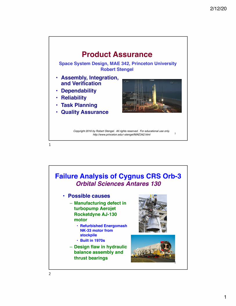
2/12/20

1

Copyright 2016 by Robert Stengel. All rights reserved. For educational use only.http://www.princeton.edu/~stengel/MAE342.html

Product AssuranceSpace System Design, MAE 342, Princeton University

Robert Stengel

• Assembly, Integration, and Verification

• Dependability• Reliability• Task Planning• Quality Assurance

1

1

Failure Analysis of Cygnus CRS Orb-3Orbital Sciences Antares 130

• Possible causes– Manufacturing defect in

turbopump AerojetRocketdyne AJ-130 motor

• Refurbished EnergomashNK-33 motor from stockpile

• Built in 1970s– Design flaw in hydraulic

balance assembly and thrust bearings

2

2

2/12/20

2

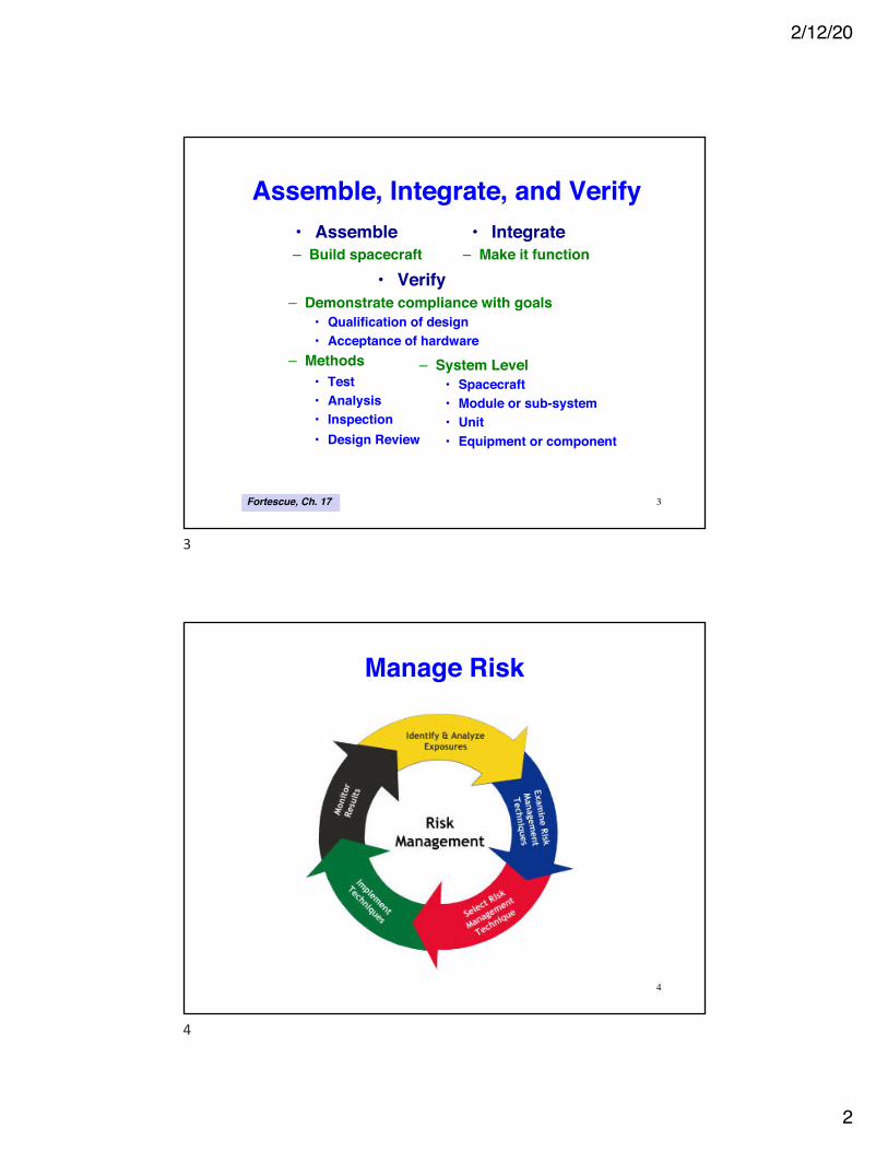
Assemble, Integrate, and Verify

• Verify– Demonstrate compliance with goals

• Qualification of design• Acceptance of hardware

– Methods• Test• Analysis• Inspection• Design Review

3

– System Level• Spacecraft• Module or sub-system• Unit• Equipment or component

Fortescue, Ch. 17

• Integrate– Make it function

• Assemble– Build spacecraft

3

Manage Risk

4

4

2/12/20

3

Classify Risk

5http://www.riskbusinessamericas.com/Public.IndustryRiskProfiles.aspx

5

6http://www.riskbusinessamericas.com/Public.IndustryRiskProfiles.aspx

Assess Risk

6

2/12/20

4

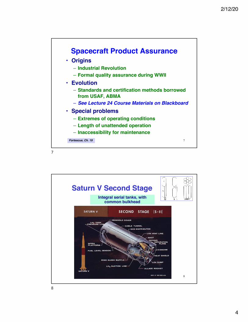
Spacecraft Product Assurance• Origins

– Industrial Revolution– Formal quality assurance during WWII

• Evolution– Standards and certification methods borrowed

from USAF, ABMA– See Lecture 24 Course Materials on Blackboard

• Special problems– Extremes of operating conditions– Length of unattended operation– Inaccessibility for maintenance

7Fortescue, Ch. 19

7

Saturn V Second StageIntegral serial tanks, with

common bulkhead

8

8

2/12/20

5

9

9

Principles and Definitions for Product Assurance

• Quality• Basis for quality assessment• Proof of quality

10Fortescue, Ch. 19

10

2/12/20

6

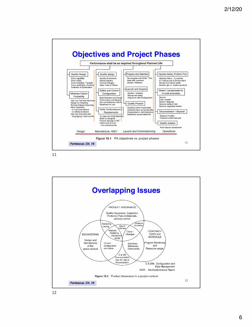
Objectives and Project Phases

11Fortescue, Ch. 19

11

Overlapping Issues

12Fortescue, Ch. 19

12

2/12/20

7

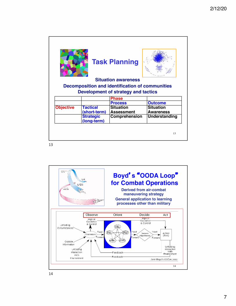
Task Planning

Situation awarenessDecomposition and identification of communities

Development of strategy and tacticsPhaseProcess Outcome

Objective Tactical (short-term)

Situation Assessment

Situation Awareness

Strategic (long-term)

Comprehension Understanding

13

13

Boyd’s “OODA Loop”for Combat Operations

Derived from air-combat maneuvering strategy

General application to learning processes other than military

14

14

2/12/20

8

Endsley, 1995

Elements of Situation Awareness

• Perception• Comprehension• Projection

15

15

Important Dichotomies in Planning

Strength, Weakness, Opportunity, and Threat (SWOT) Analysis “Knok-Knoks” and “Unk-

Unks”

16

16

2/12/20

9

Program Management: Gantt ChartProject schedule

Task breakdown and dependencyStart, interim, and finish elements

Time elapsed, time to go

17

17

Program Evaluation and Review Technique (PERT) Chart

MilestonesPath descriptors

Activities, precursors, and successorsTiming and coordination

Identification of critical pathOptimization and constraint

18

18

2/12/20

10

-ilities• Dependability

– Availability– Maintainability– Security

• Reliability– Qualitative– Quantitative– Design or predicted– Operational

19

19

Parts Procurement• Vendors’ track record• Standardization• Procurement systems

– Organization– Documentation

• Substitution of less reliable equivalents

• Out-of-date/specification parts20

20

2/12/20

11

Materials and Processes

21Fortescue, Ch. 19

21

Materials to Avoid

22Fortescue, Ch. 19

22

2/12/20

12

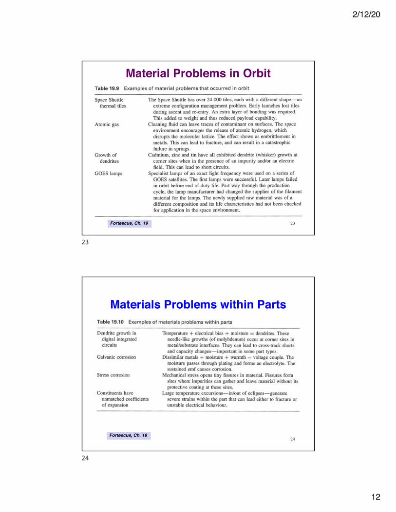
Material Problems in Orbit

23Fortescue, Ch. 19

23

Materials Problems within Parts

24Fortescue, Ch. 19

24

2/12/20

13

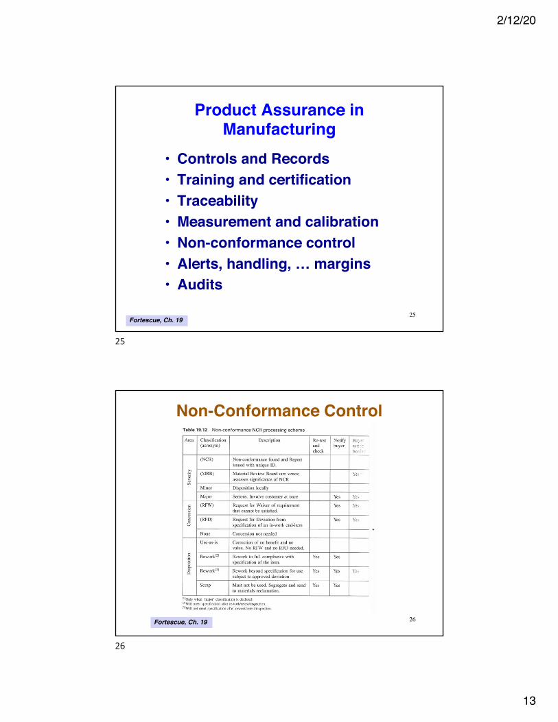
Product Assurance in Manufacturing

• Controls and Records• Training and certification• Traceability• Measurement and calibration• Non-conformance control• Alerts, handling, … margins• Audits

25Fortescue, Ch. 19

25

Non-Conformance Control

26Fortescue, Ch. 19

26

2/12/20

14

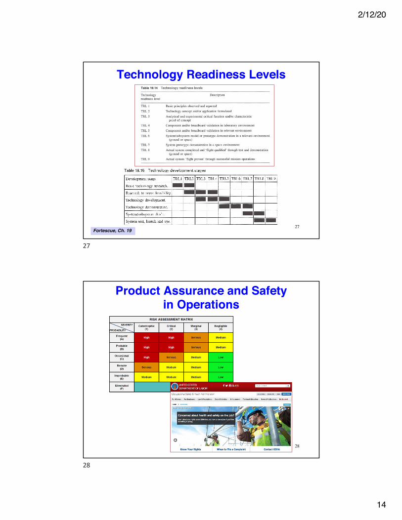
Technology Readiness Levels

27Fortescue, Ch. 19

27

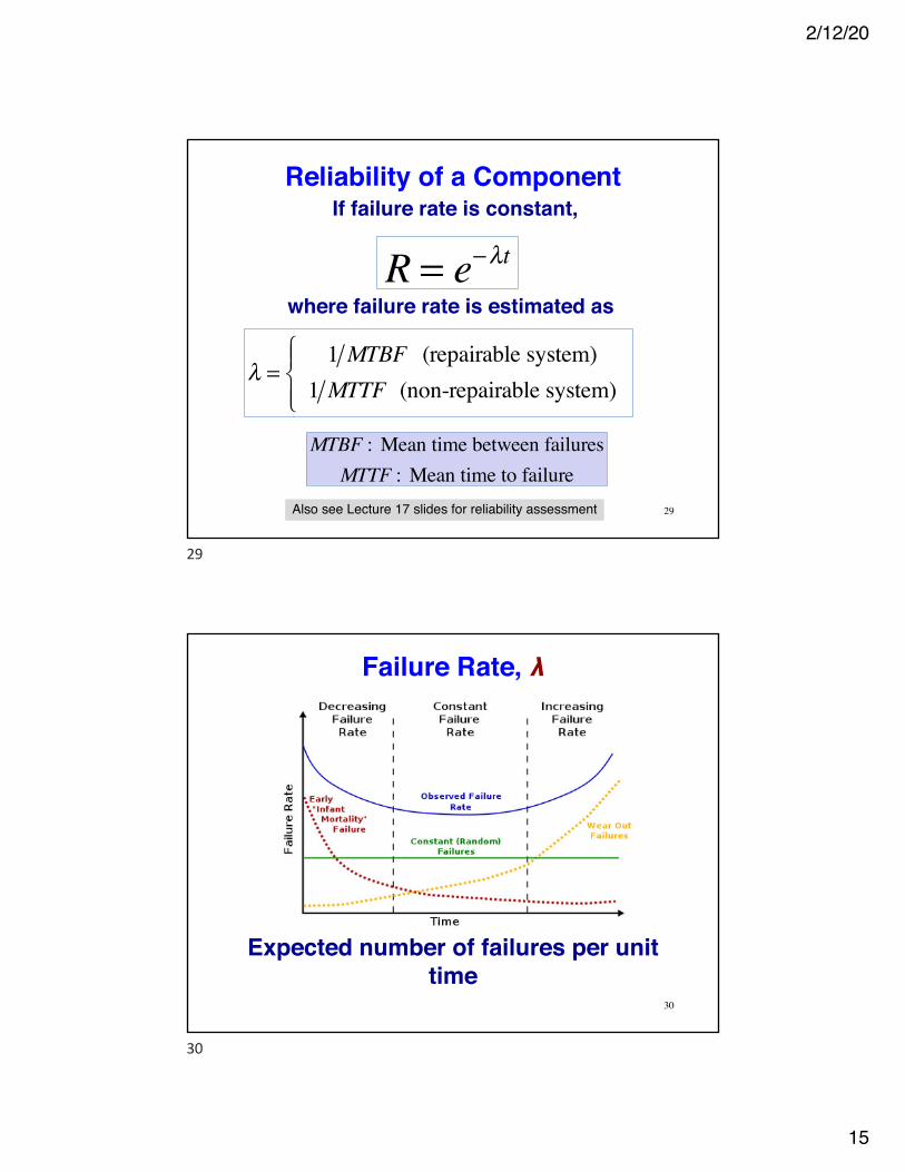
Product Assurance and Safety in Operations

28

28

2/12/20

15

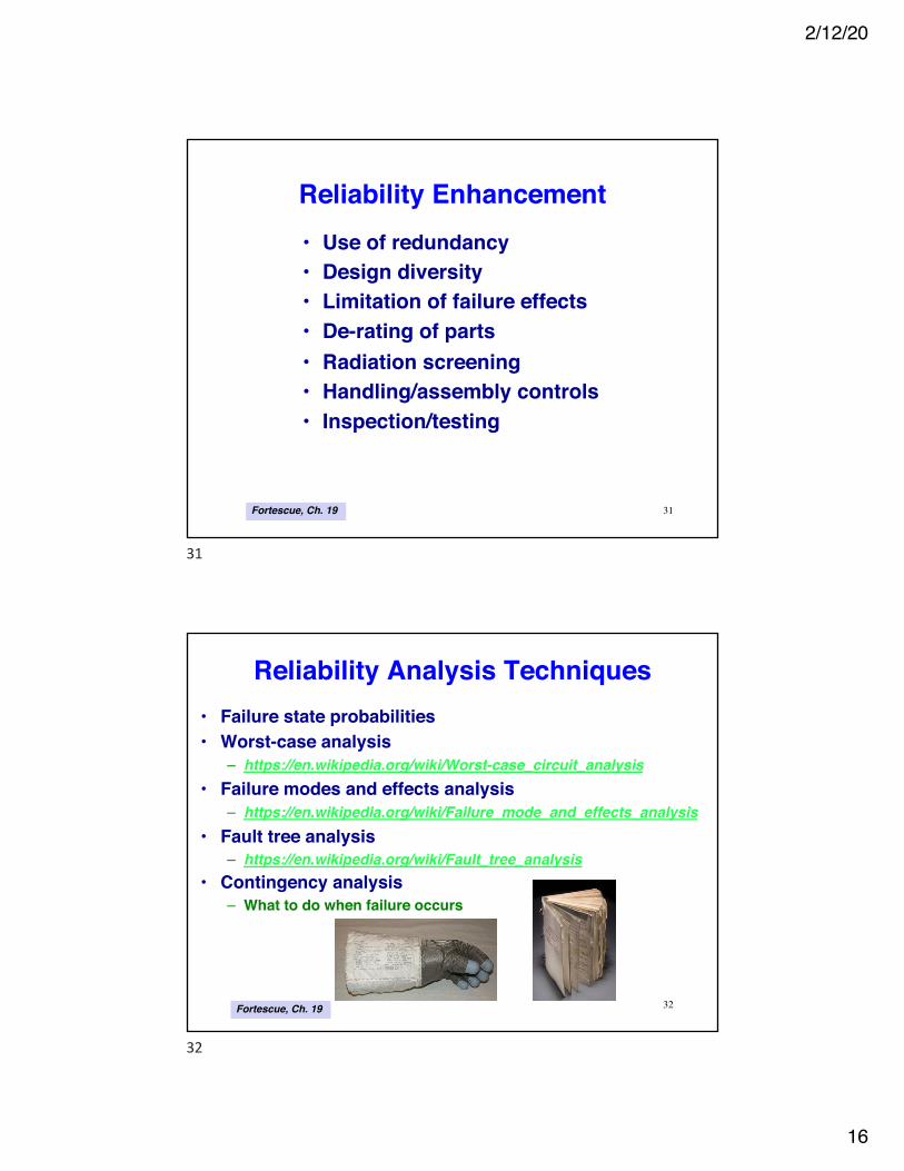
Reliability of a Component

29

R = e−λtIf failure rate is constant,

Also see Lecture 17 slides for reliability assessment

where failure rate is estimated as

λ =1 MTBF (repairable system)

1 MTTF (non-repairable system)

⎧⎨⎪

⎩⎪

MTBF : Mean time between failuresMTTF : Mean time to failure

29

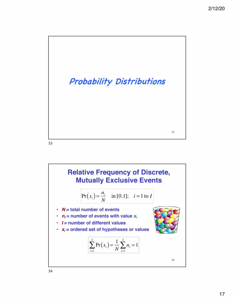
Failure Rate, λ

30

Expected number of failures per unit time

30

2/12/20

16

Reliability Enhancement• Use of redundancy• Design diversity• Limitation of failure effects• De-rating of parts• Radiation screening• Handling/assembly controls• Inspection/testing

31Fortescue, Ch. 19

31

Reliability Analysis Techniques• Failure state probabilities• Worst-case analysis

– https://en.wikipedia.org/wiki/Worst-case_circuit_analysis• Failure modes and effects analysis

– https://en.wikipedia.org/wiki/Failure_mode_and_effects_analysis• Fault tree analysis

– https://en.wikipedia.org/wiki/Fault_tree_analysis• Contingency analysis

– What to do when failure occurs

32Fortescue, Ch. 19

32

2/12/20

17

Probability Distributions

33

33

Relative Frequency of Discrete, Mutually Exclusive Events

• N = total number of events• ni = number of events with value xi

• I = number of different values• xi = ordered set of hypotheses or values

Pr xi( ) = niN

in [0,1]; i = 1 to I

34

Pr xi( )i=1

I

∑ = 1N

nii=1

I

∑ = 1

34

2/12/20

18

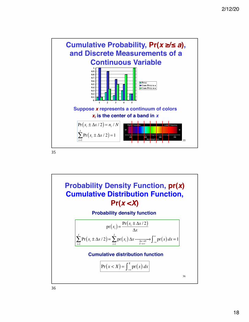
Cumulative Probability, Pr(x ≥/≤ a), and Discrete Measurements of a

Continuous Variable

Suppose x represents a continuum of colorsxi is the center of a band in x

00.10.20.30.40.50.60.70.80.9

1

1 2 3 4 5

Pr(x)Cum Pr(x) ≥ aCum Pr(x) ≤ a

Pr xi ± Δx / 2( ) = ni / N

Pr xi ± Δx / 2( ) = 1i=1

I

∑35

35

Probability Density Function, pr(x)Cumulative Distribution Function,

Pr(x <X)Probability density function

Pr x < X( ) = pr x( ) dx−∞

X

∫

Cumulative distribution function

pr xi( ) = Pr xi ± Δx / 2( )Δx

Pr xi ± Δx / 2( ) = pr xi( ) Δxi=1

I

∑ Δx→0I→∞

⎯ →⎯⎯ pr x( ) dx−∞

∞

∫ = 1i=1

I

∑

36

36

2/12/20

19

Probability Density Function, pr(x) Cumulative Distribution Function,

Pr(x <X)

Pr x < X( ) = pr x( ) dx−∞

X

∫

37

37

Properties of Random Variables

• Mode– Value of x for which pr(x) is maximum

x = E(x) = x pr x( ) dx−∞

∞

∫

• Median– Value of x corresponding to 50th percentile– Pr(x < median) = Pr(x ≥ median) = 0.5

• Mean– Value of x corresponding to statistical average

• First moment of x = Expected value of x

“Moment arm”

“Force”

38

38

2/12/20

20

Expected Values

• Second central moment of x = Variance– Variance from the mean value rather than from zero– Smaller value indicates less uncertainty in the value

of x

σ x2 = E x − x( )2⎡⎣ ⎤⎦ = x − x( )2 pr x( ) dx

−∞

∞

∫

x = E(x) = x pr x( ) dx−∞

∞

∫

• Mean Value is the first moment of x

39

39

Mean Value and Variance of a Uniform Distribution

Variance

If xmin = −xmax ! a

σ x2 = 1

2ax2 dx

−a

a

∫ = x3

6a −a

a

= a2

3 40

pr(x) =

01

xmax − xmin0

;x < xmin

xmin < x < xmaxx > xmax

⎧

⎨⎪⎪

⎩⎪⎪

x = xxmax − xmin( ) dxxmin

xmax∫ = 12xmax + xmin( )

Mean

40

2/12/20

21

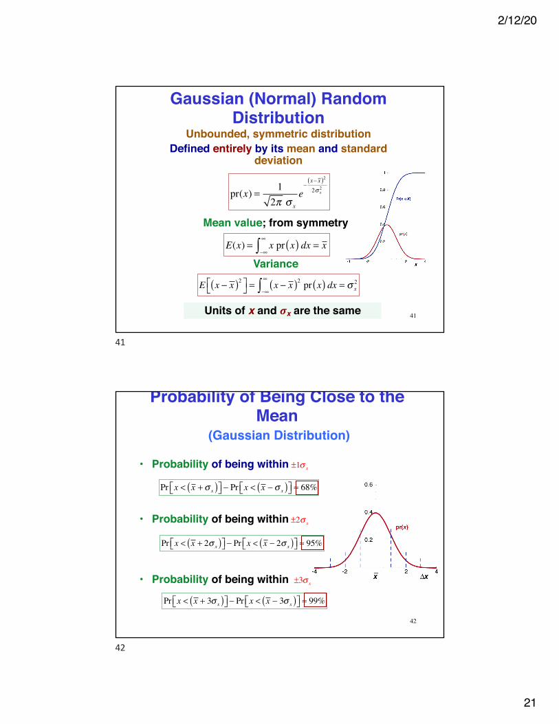
Gaussian (Normal) Random Distribution

pr(x) = 12π σ x

e−x− x( )2

2σ x2

E(x) = x pr x( ) dx−∞

∞

∫ = x

Variance

Units of x and σx are the same

Unbounded, symmetric distributionDefined entirely by its mean and standard

deviation

E x − x( )2⎡⎣ ⎤⎦ = x − x( )2 pr x( ) dx−∞

∞

∫ = σ x2

Mean value; from symmetry

41

41

Probability of Being Close to the Mean

(Gaussian Distribution)

• Probability of being within

Pr x < x +σ x( )⎡⎣ ⎤⎦ − Pr x < x − σ x( )⎡⎣ ⎤⎦ ≈ 68%

• Probability of being within

• Probability of being within

Pr x < x + 2σ x( )⎡⎣ ⎤⎦ − Pr x < x − 2σ x( )⎡⎣ ⎤⎦ ≈ 95%

Pr x < x + 3σ x( )⎡⎣ ⎤⎦ − Pr x < x − 3σ x( )⎡⎣ ⎤⎦ ≈ 99%

±1σ x

±2σ x

±3σ x

42

42

2/12/20

22

Experimental Determination of Mean and Variance

Divisor is (N – 1) rather than N to produce an unbiased estimate

x =xi

i=1

N

∑N

Sample variance for same data set

σ x2 =

xi − x( )2i=1

N

∑N −1( )

Sample mean for N data points, x1, x2, ..., xN

Histogram

43

43

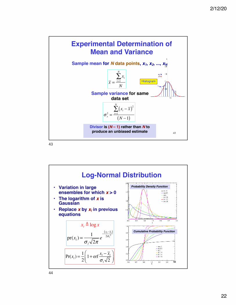
Log-Normal Distribution

xl ! log x

pr(xl ) =1

σ l 2πe−xl−xl( )2σ l

2

• Variation in large ensembles for which x > 0

• The logarithm of x is Gaussian

• Replace x by xl in previous equations

Pr(xl ) =121+ erf xl − xl

σ l 2⎛⎝⎜

⎞⎠⎟

Probability Density Function

Cumulative Probability Function

44

44

2/12/20

23

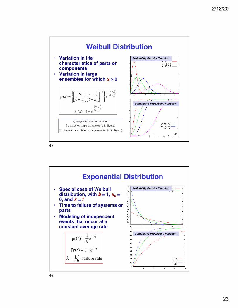
Weibull Distribution

pr(x) = bθ − xo

⎡

⎣⎢

⎤

⎦⎥x − xoθ − xo

⎡

⎣⎢

⎤

⎦⎥

b−1⎧⎨⎪

⎩⎪

⎫⎬⎪

⎭⎪e−x−xo( )bθ−xo( )b

Pr(x) = 1− e−x−xo( )bθ−xo( )b

• Variation in life characteristics of parts or components

• Variation in large ensembles for which x > 0

Probability Density Function

Cumulative Probability Function

xo : expected minimum valueb : shape or slope parameter (k in figure)

θ : characteristic life or scale parameter (λ in figure)45

45

Exponential Distribution

pr(t) = 1θe−

tθ

Pr(t) = 1− e−tθ

λ = 1θ : failure rate

• Special case of Weibulldistribution, with b = 1, xo = 0, and x = t

• Time to failure of systems or parts

• Modeling of independent events that occur at a constant average rate

Probability Density Function

Cumulative Probability Function

46

46

2/12/20

24

Poisson Distribution

pr(r = ri ) =e−λyri

ri !

• Occurrence of isolated, independent events whose average rate is known– Number of events can be

observed– Number of non-events cannot be

observed• Examples:

– Number of machine breakdowns in a plant

– Number of errors in a drawing

Probability Mass Function

Cumulative Probability Function

λ : average number of occurrences47

47

Binomial Distribution

�

pr(r) =nr

⎛

⎝ ⎜ ⎞

⎠ ⎟ prqn−r =

nr

⎛

⎝ ⎜ ⎞

⎠ ⎟ pr 1− p( )n−r

wherenr

⎛

⎝ ⎜ ⎞

⎠ ⎟ = n!

r! n − r( )!n = number of trialsp = probability of successq = probability of failure

• The probability of rsuccessful outcomes in ntrials

• Examples: inspection of parts, probability that a system will operate correctly

Probability Mass Function

Cumulative Probability Function

48

48

2/12/20

25

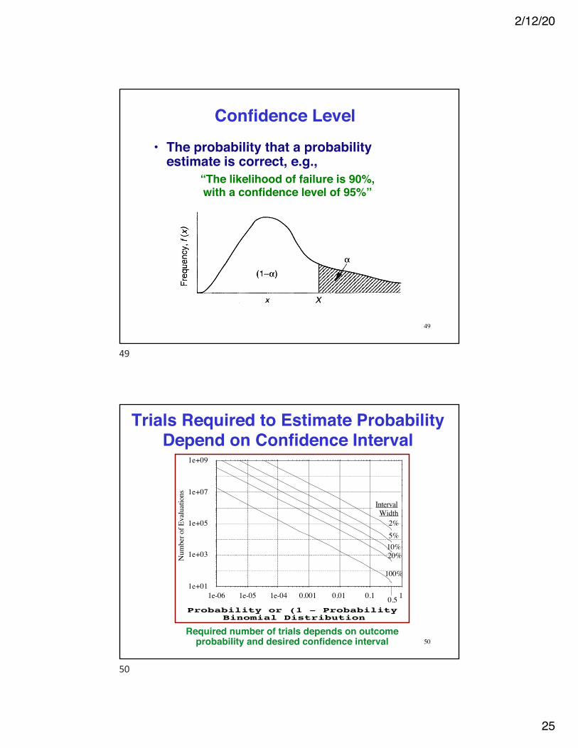
Confidence Level• The probability that a probability

estimate is correct, e.g.,

49

“The likelihood of failure is 90%, with a confidence level of 95%”

49

Trials Required to Estimate Probability Depend on Confidence Interval

1e+01

1e+03

1e+05

1e+07

1e+09

1e-06 1e-05 1e-04 0.001 0.01 0.1 1

2%5%10%20%

100%

Num

ber o

f Eva

luat

ions

0.5

IntervalWidth

Probability or (1 - Probability)Binomial Distribution

Required number of trials depends on outcome probability and desired confidence interval 50

50

2/12/20

26

How Will You Estimate the Likelihood of Success for Project

2020 UA?

51

51

52

MAE 342, Space System Design

52

2/12/20

27

53

53