22s:152 Applied Linear Regression Chapter 13: Multicollinearity

22s:152 Applied Linear Regression

Chapter 13:Multicollinearity————————————————————

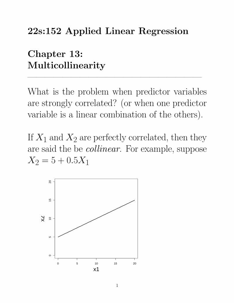
What is the problem when predictor variablesare strongly correlated? (or when one predictorvariable is a linear combination of the others).

If X1 and X2 are perfectly correlated, then theyare said the be collinear. For example, supposeX2 = 5 + 0.5X1

0 5 10 15 20

05

1015

20

x1

x2

1

Multicollinearity is the situation where one ormore predictor variables are “nearly” linearlyrelated to the others.

If one of the predictors is almost perfectly pre-dicted from the set of other variables, then youhave multicollinearity.

How does this affect an analysis?

2

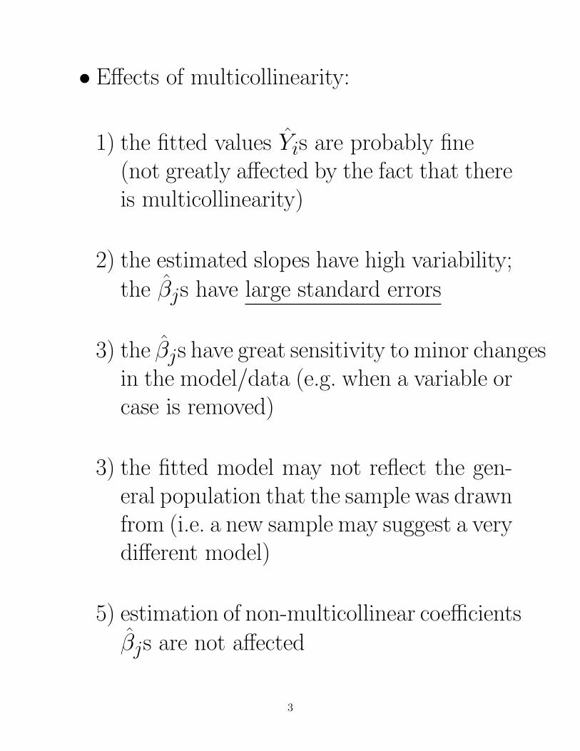
• Effects of multicollinearity:

1) the fitted values Yis are probably fine(not greatly affected by the fact that thereis multicollinearity)

2) the estimated slopes have high variability;the βjs have large standard errors

3) the βjs have great sensitivity to minor changesin the model/data (e.g. when a variable orcase is removed)

3) the fitted model may not reflect the gen-eral population that the sample was drawnfrom (i.e. a new sample may suggest a verydifferent model)

5) estimation of non-multicollinear coefficientsβjs are not affected

3

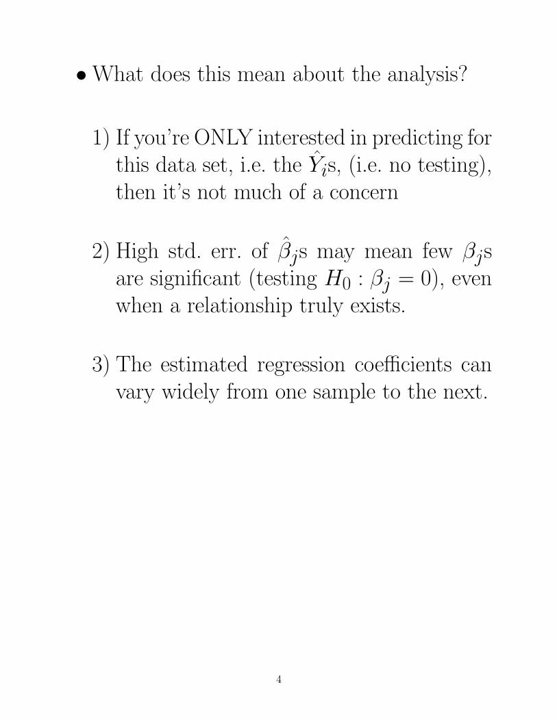
• What does this mean about the analysis?

1) If you’re ONLY interested in predicting forthis data set, i.e. the Yis, (i.e. no testing),then it’s not much of a concern

2) High std. err. of βjs may mean few βjsare significant (testing H0 : βj = 0), evenwhen a relationship truly exists.

3) The estimated regression coefficients canvary widely from one sample to the next.

4

How does high correlation in your predictor vari-ables lead to unstable estimates of the βjs?

Example: Consider a hypothetical situation...

• Suppose we’re measuring the white blood-cell count (WBC) in a population of sick pa-tients (the response, as count per microliterof blood).

• Higher white blood cell counts coincide withsicker patients.

• We also have measures on two other quanti-ties in the body:

1) quantity of Organism A in the body, X1

2) quantity of Organism B in the body, X2

The researchers don’t know it, but OrganismA attacks the body (and increases WBC),and Organism B is inert (a harmless by-productof Organism A).

5

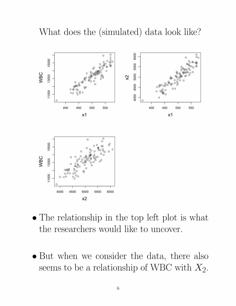
What does the (simulated) data look like?

400 450 500 550

11000

13000

15000

x1

WBC

400 450 500 550

4000

4500

5000

5500

6000

x1

x2

4000 4500 5000 5500 6000

11000

13000

15000

x2

WBC

• The relationship in the top left plot is whatthe researchers would like to uncover.

• But when we consider the data, there alsoseems to be a relationship of WBC with X2.

6

• Generate 10 simulated data sets,and fit the model using both predictors:

Std. p Std. p

Run β1 error value β2 error value

1 21.89 20.19 0.28 0.36 2.00 0.86

2 -16.75 22.51 0.46 4.14 2.24 0.07

3 20.33 17.98 0.26 0.53 1.80 0.77

4 25.82 16.09 0.11 0.05 1.60 0.98

5 4.87 21.36 0.82 1.95 2.14 0.36

6 38.61 19.30 0.05 -1.40 1.93 0.47

7 -3.92 19.90 0.84 3.10 1.98 0.12

8 46.74 23.98 0.05 -2.19 2.41 0.37

9 -10.74 17.45 0.54 3.65 1.75 0.04

10 40.90 18.12 0.03 -1.48 1.83 0.42

• The βs are very variable (they change a lotfrom one simulation to the next).

• The signs on βs are even sometimes “−”

• Tests of H0 : βj = 0 are not often significant(eventhough a relationship exists).

• Our interpretation of MLR coefficients is lostwhen multicollinearity exists because we can’thold one variable constant while changingthe other (they MUST move simultaneously).

7

Visual of instability of coefficients

If we have instability of coefficient estimates,then the fitted plane is very dependent on theparticular sample chosen. See the 4 runs below:

WBC vs. x1 and x2

350 400 450 500 550 600 650 700100110120130140150160170

400045005000550060006500

x1

x2WB

C (1

/100

sca

le)

WBC vs. x1 and x2

350 400 450 500 550 600 650 700100110120130140150160170

400045005000550060006500

x1

x2WB

C (1

/100

sca

le)

WBC vs. x1 and x2

350 400 450 500 550 600 650 700100110120130140150160170

400045005000550060006500

x1

x2WB

C (1

/100

sca

le)

WBC vs. x1 and x2

350 400 450 500 550 600 650 700100110120130140150160170

400045005000550060006500

x1

x2WB

C (1

/100

sca

le)

8

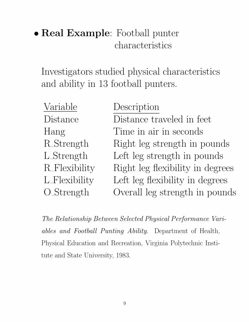
•Real Example: Football puntercharacteristics

Investigators studied physical characteristicsand ability in 13 football punters.

Variable DescriptionDistance Distance traveled in feetHang Time in air in secondsR Strength Right leg strength in poundsL Strength Left leg strength in poundsR Flexibility Right leg flexibility in degreesL Flexibility Left leg flexibility in degreesO Strength Overall leg strength in pounds

The Relationship Between Selected Physical Performance Vari-

ables and Football Punting Ability. Department of Health,

Physical Education and Recreation, Virginia Polytechnic Insti-

tute and State University, 1983.

9

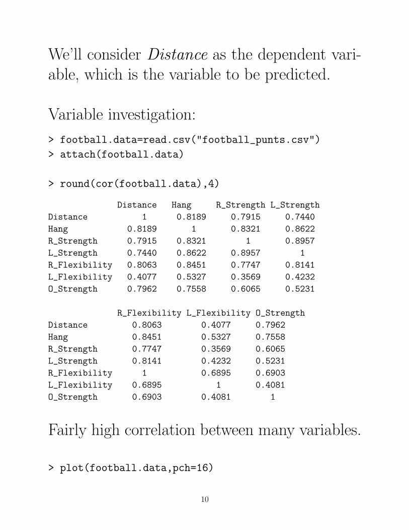
We’ll consider Distance as the dependent vari-able, which is the variable to be predicted.

Variable investigation:

> football.data=read.csv("football_punts.csv")

> attach(football.data)

> round(cor(football.data),4)

Distance Hang R_Strength L_Strength

Distance 1 0.8189 0.7915 0.7440

Hang 0.8189 1 0.8321 0.8622

R_Strength 0.7915 0.8321 1 0.8957

L_Strength 0.7440 0.8622 0.8957 1

R_Flexibility 0.8063 0.8451 0.7747 0.8141

L_Flexibility 0.4077 0.5327 0.3569 0.4232

O_Strength 0.7962 0.7558 0.6065 0.5231

R_Flexibility L_Flexibility O_Strength

Distance 0.8063 0.4077 0.7962

Hang 0.8451 0.5327 0.7558

R_Strength 0.7747 0.3569 0.6065

L_Strength 0.8141 0.4232 0.5231

R_Flexibility 1 0.6895 0.6903

L_Flexibility 0.6895 1 0.4081

O_Strength 0.6903 0.4081 1

Fairly high correlation between many variables.

> plot(football.data,pch=16)

10

Distance

3.0 3.5 4.0 4.5

●

●●

●

●

●

●

●●

●

●

●

● ●

●●

●

●

●

●

● ●

●

●

●

●

110 130 150 170

●

●●

●

●

●

●

●●

●

●

●

● ●

●●

●

●

●

●

● ●

●

●

●

●

80 90 100

●

●●

●

●

●

●

●●

●

●

●

●

120

160●

●●

●

●

●

●

●●

●

●

●

●

3.0

3.5

4.0

4.5

●

●●

●

●

●

●

●

●

● ●●

● Hang

●

● ●

●

●

●

●

●

●

●●●

●

●

● ●

●

●

●

●

●

●

● ●●

●

●

●●

●

●

●

●

●

●

● ●●

●

●

●●

●

●

●

●

●

●

● ●●

●

●

●●

●

●

●

●

●

●

●●●

●

●

●

●

●

●

●

●

●

●

●

●

●

●

●

●

●

●

●

●

●

●

●

●

●

●

●

R_Strength

●

●

●

●

●

●

●

●

●

●

●

●

●

●

●

●

●

●

●

●

●

●

●

●

●

●

●

●

●

●

●

●

●

●

●

●

●

●

●

110

130

150

170

●

●

●

●

●

●

●

●

●

●

●

●

●

110

130

150

170

●

●

●

●

●●

●

●●

●

●

●

●

●

●

●

●

●●

●

●●

●

●

●

●

●

●

●

●

●●

●

● ●

●

●

●

● L_Strength

●

●

●

●

●●

●

● ●

●

●

●

●

●

●

●

●

●●

●

●●

●

●

●

●

●

●

●

●

●●

●

●●

●

●

●

●

●

●●

●●

●

●

●

●

●

●

●

●

●

●●

●●

●

●

●

●

●

●

●

●

●

●●

●●

●

●

●

●

●

●

●

●

●

●●

●●

●

●

●

●

●

●

●

●R_Flexibility

●

●●

●●

●

●

●

●

●

●

●

●

8590

9510

5●

●●

●●

●

●

●

●

●

●

●

●

8090

100

●

●

●

● ●

●

●

●

●

●

●

●●

●

●

●

● ●

●

●

●

●

●

●

●●

●

●

●

● ●

●

●

●

●

●

●

●●

●

●

●

●●

●

●

●

●

●

●

●●

●

●

●

●●

●

●

●

●

●

●

●●

L_Flexibility

●

●

●

● ●

●

●

●

●

●

●

●●

120 160

●

●

●

●

●●

●

●●

●

● ●

● ●

●

●

●

●●

●

●●

●

●●

●

110 130 150 170

●

●

●

●

●●

●

● ●

●

● ●

● ●

●

●

●

●●

●

●●

●

●●

●

85 90 95 105

●

●

●

●

●●

●

● ●

●

● ●

● ●

●

●

●

●●

●

●●

●

● ●

●

140 180 220 260

140

180

220

260

O_Strength

Linearity looks reasonable, except for the leftflexibility variable. This variable seems to havesome outliers, and has the lowest correlationwith the other variables (most kickers are right-footed?)

11

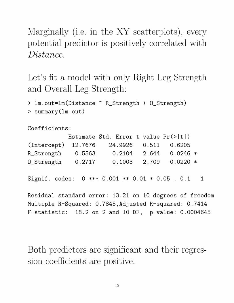
Marginally (i.e. in the XY scatterplots), everypotential predictor is positively correlated withDistance.

Let’s fit a model with only Right Leg Strengthand Overall Leg Strength:

> lm.out=lm(Distance ~ R_Strength + O_Strength)

> summary(lm.out)

Coefficients:

Estimate Std. Error t value Pr(>|t|)

(Intercept) 12.7676 24.9926 0.511 0.6205

R_Strength 0.5563 0.2104 2.644 0.0246 *

O_Strength 0.2717 0.1003 2.709 0.0220 *

---

Signif. codes: 0 *** 0.001 ** 0.01 * 0.05 . 0.1 1

Residual standard error: 13.21 on 10 degrees of freedom

Multiple R-Squared: 0.7845,Adjusted R-squared: 0.7414

F-statistic: 18.2 on 2 and 10 DF, p-value: 0.0004645

Both predictors are significant and their regres-sion coefficients are positive.

12

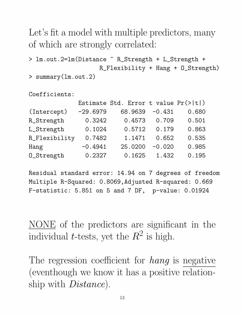
Let’s fit a model with multiple predictors, manyof which are strongly correlated:

> lm.out.2=lm(Distance ~ R_Strength + L_Strength +

R_Flexibility + Hang + O_Strength)

> summary(lm.out.2)

Coefficients:


(Intercept) -29.6979 68.9639 -0.431 0.680

R_Strength 0.3242 0.4573 0.709 0.501

L_Strength 0.1024 0.5712 0.179 0.863

R_Flexibility 0.7482 1.1471 0.652 0.535

Hang -0.4941 25.0200 -0.020 0.985

O_Strength 0.2327 0.1625 1.432 0.195




NONE of the predictors are significant in theindividual t-tests, yet the R2 is high.

The regression coefficient for hang is negative(eventhough we know it has a positive relation-ship with Distance).

13

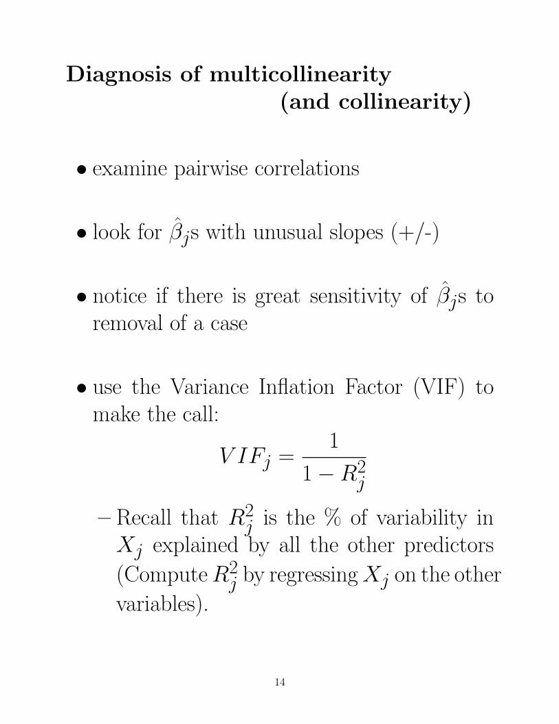
Diagnosis of multicollinearity(and collinearity)

• examine pairwise correlations

• look for βjs with unusual slopes (+/-)

• notice if there is great sensitivity of βjs toremoval of a case

• use the Variance Inflation Factor (VIF) tomake the call:

V IFj =1

1−R2j

– Recall that R2j is the % of variability in

Xj explained by all the other predictors

(ComputeR2j by regressingXj on the other

variables).

14

V IFj =1

1−R2j

– When R2j is close to 1 (i.e. you can predict

Xj very well from the other predictors),V IFj will be large.

– V IF > 10 indicates a problem

– V IF > 100 indicates a BIG problem

COMMENT: The slopes have specific units, sofinding the largest standard error does not nec-essarily mean you’ve found the variable with thelargest VIF.

15

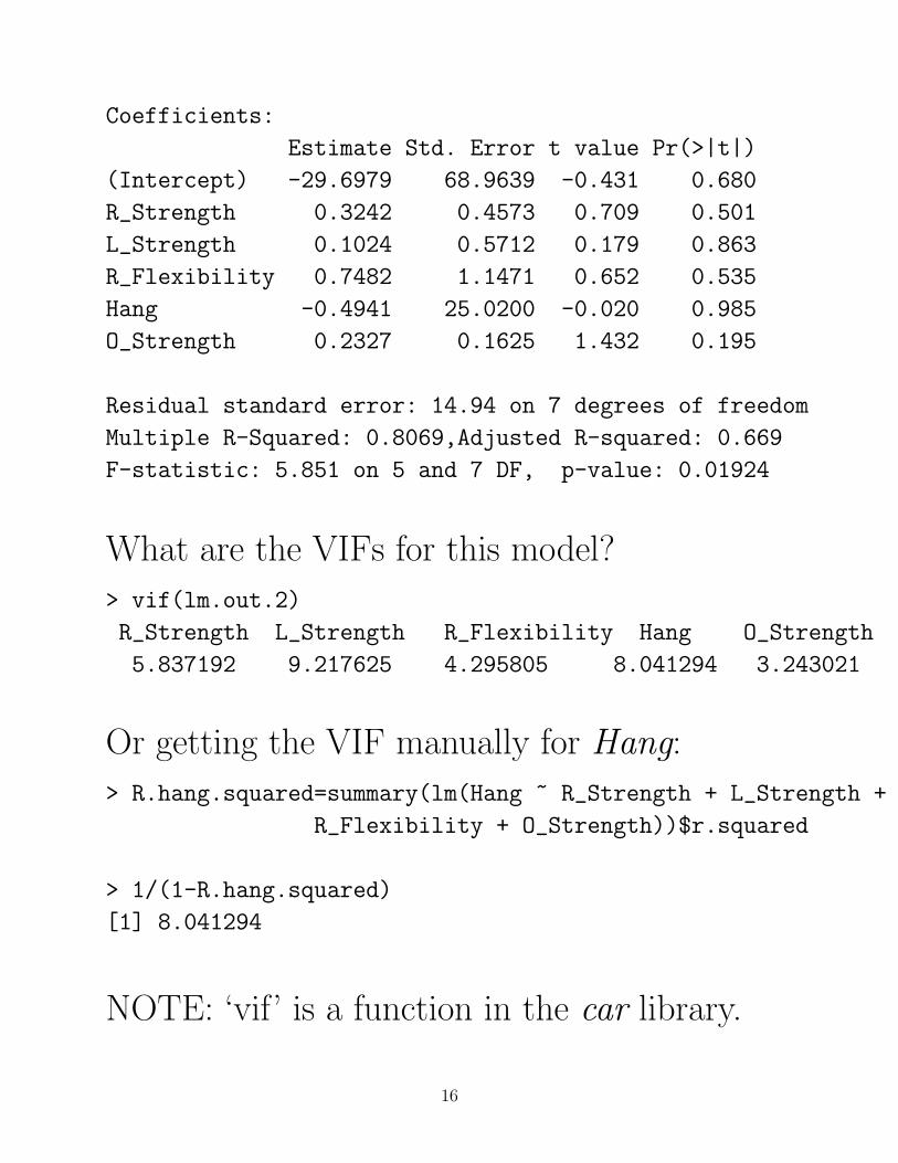
Coefficients:


(Intercept) -29.6979 68.9639 -0.431 0.680

R_Strength 0.3242 0.4573 0.709 0.501

L_Strength 0.1024 0.5712 0.179 0.863

R_Flexibility 0.7482 1.1471 0.652 0.535

Hang -0.4941 25.0200 -0.020 0.985

O_Strength 0.2327 0.1625 1.432 0.195




What are the VIFs for this model?

> vif(lm.out.2)

R_Strength L_Strength R_Flexibility Hang O_Strength

5.837192 9.217625 4.295805 8.041294 3.243021

Or getting the VIF manually for Hang:

> R.hang.squared=summary(lm(Hang ~ R_Strength + L_Strength +

R_Flexibility + O_Strength))$r.squared

> 1/(1-R.hang.squared)

[1] 8.041294

NOTE: ‘vif’ is a function in the car library.

16

Remedies of multicollinearity(and collinearity)

• Could use the model only for prediction Yis(but probably not so useful)

WBC vs. x1 and x2

350 400 450 500 550 600 650 700100110120130140150160170

400045005000550060006500

x1

x2WB

C (1

/100

sca

le)

WBC vs. x1 and x2

350 400 450 500 550 600 650 700100110120130140150160170

400045005000550060006500

x1

x2WB

C (1

/100

sca

le)

Notice how the fitted planes may be quite dif-ferent, but the predicted values in the realmof observed (x1, x2) combinations don’t changemuch.

• Drop variables that are highly correlated(there are choices to be made here)

17

• Create composite (combined) variables:

i) If X1, X2, and X3 are strongly correlated,use Xnew = 0.25X1 + 0.25X2 + 0.50X3

ii) Principal components analysis

These are dimension reduction techniques.

• Use Ridge Regression which will introducesome bias to the regression coefficient esti-mates, but can greatly reduce the standarderrors.

18

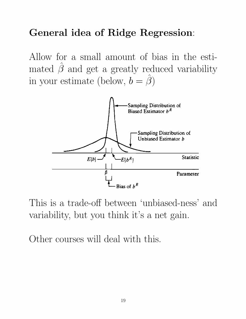
General idea of Ridge Regression:

Allow for a small amount of bias in the esti-mated β and get a greatly reduced variabilityin your estimate (below, b = β)

This is a trade-off between ‘unbiased-ness’ andvariability, but you think it’s a net gain.

Other courses will deal with this.

19

Multicollinearity (and Collinearity)

• It is not an assumption violation, but it isimportant to check for it.

• The problem can be a pair of highly corre-lated variables, or a large group of moder-ately correlated variables.

• It can cause a lot of problems in an analysis.

• Inclusion of interaction terms introduces somecollinearity to a model, but their inclusion isnecessary if the interaction effect is impor-tant.

20

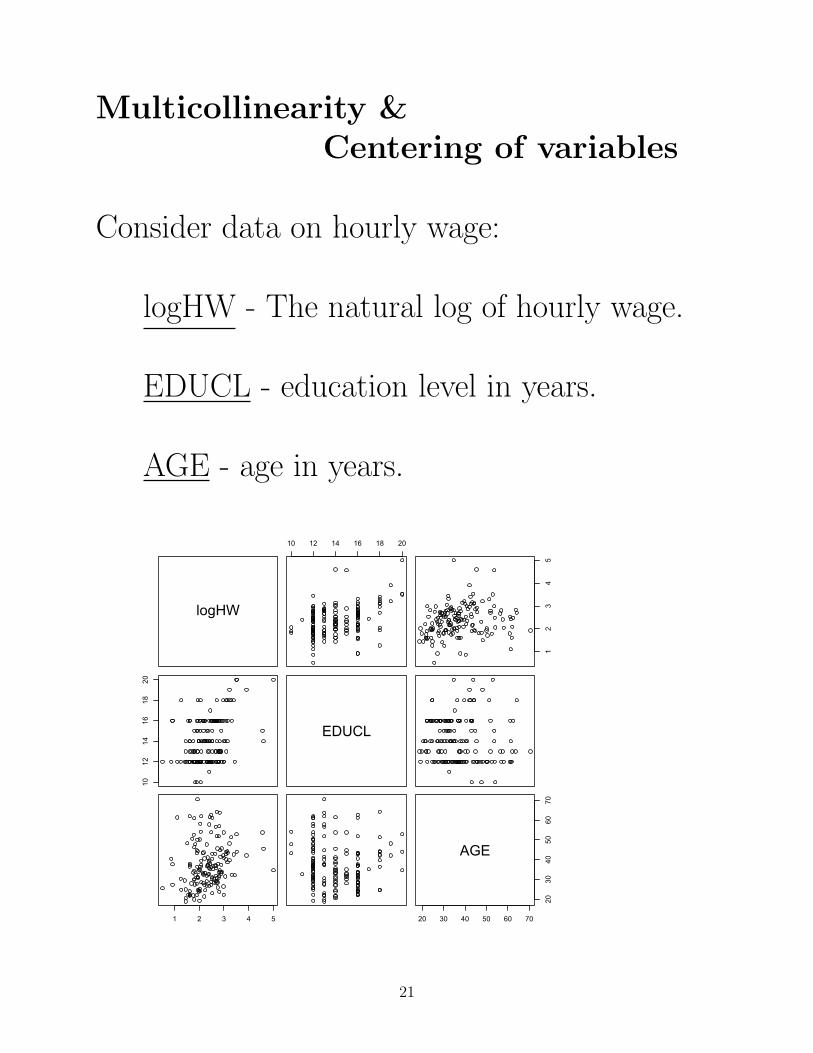
Multicollinearity &Centering of variables

Consider data on hourly wage:

logHW - The natural log of hourly wage.

EDUCL - education level in years.

AGE - age in years.

logHW

10 12 14 16 18 201

23

45

1012

1416

1820

EDUCL

1 2 3 4 5 20 30 40 50 60 70

2030

4050

6070

AGE

21

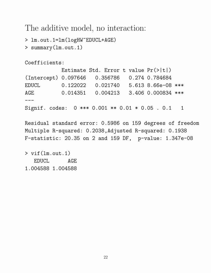
The additive model, no interaction:

> lm.out.1=lm(logHW~EDUCL+AGE)

> summary(lm.out.1)

Coefficients:


(Intercept) 0.097646 0.356786 0.274 0.784684

EDUCL 0.122022 0.021740 5.613 8.66e-08 ***

AGE 0.014351 0.004213 3.406 0.000834 ***

---

Signif. codes: 0 *** 0.001 ** 0.01 * 0.05 . 0.1 1


Multiple R-squared: 0.2038,Adjusted R-squared: 0.1938

F-statistic: 20.35 on 2 and 159 DF, p-value: 1.347e-08

> vif(lm.out.1)

EDUCL AGE

1.004588 1.004588

22

The model with interaction:

> lm.out.2=lm(logHW~EDUCL+AGE+EDUCL:AGE)

> summary(lm.out.2)

Coefficients:


(Intercept) 3.224920 1.203000 2.681 0.00813 **

EDUCL -0.101347 0.084931 -1.193 0.23455

AGE -0.063481 0.028943 -2.193 0.02975 *

EDUCL:AGE 0.005579 0.002054 2.717 0.00732 **

---

Signif. codes: 0 *** 0.001 ** 0.01 * 0.05 . 0.1 1




> vif(lm.out.2)

EDUCL AGE EDUCL:AGE

15.94743 49.31408 60.62104

Very high VIF values.

23

The additive model with centered variables:

> cent.educ=EDUCL-mean(EDUCL)

> cent.age=AGE-mean(AGE)

> lm.out.3=lm(logHW~cent.educ+cent.age)

> summary(lm.out.3)

Coefficients:


(Intercept) 2.352738 0.047030 50.026 < 2e-16 ***

cent.educ 0.122022 0.021740 5.613 8.66e-08 ***

cent.age 0.014351 0.004213 3.406 0.000834 ***

---

Signif. codes: 0 *** 0.001 ** 0.01 * 0.05 . 0.1 1




> vif(lm.out.3)

cent.educ cent.age

1.004588 1.004588

The estimated partial regression coefficients foreducation and age are exactly the same as inthe first additive model (as are the p-values).The VIFs are the same as well.

24

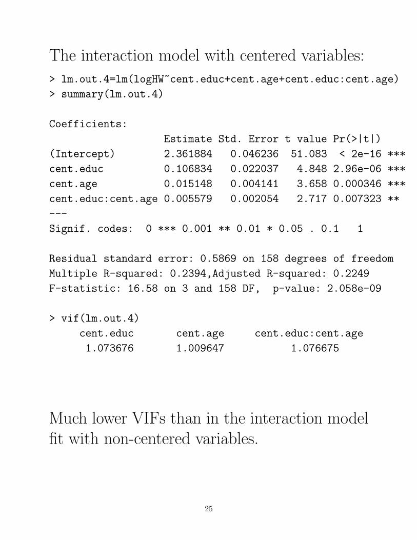
The interaction model with centered variables:

> lm.out.4=lm(logHW~cent.educ+cent.age+cent.educ:cent.age)

> summary(lm.out.4)

Coefficients:


(Intercept) 2.361884 0.046236 51.083 < 2e-16 ***

cent.educ 0.106834 0.022037 4.848 2.96e-06 ***

cent.age 0.015148 0.004141 3.658 0.000346 ***

cent.educ:cent.age 0.005579 0.002054 2.717 0.007323 **

---

Signif. codes: 0 *** 0.001 ** 0.01 * 0.05 . 0.1 1




> vif(lm.out.4)

cent.educ cent.age cent.educ:cent.age

1.073676 1.009647 1.076675

Much lower VIFs than in the interaction modelfit with non-centered variables.

25

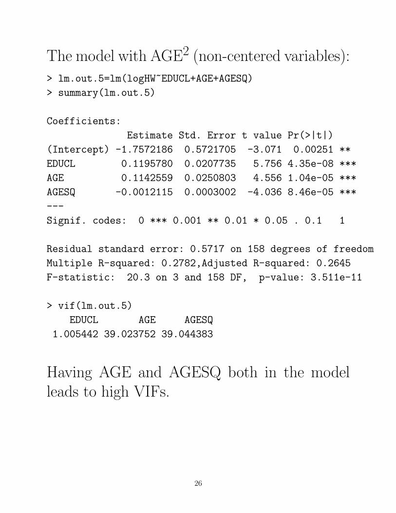
The model with AGE2 (non-centered variables):

> lm.out.5=lm(logHW~EDUCL+AGE+AGESQ)

> summary(lm.out.5)

Coefficients:


(Intercept) -1.7572186 0.5721705 -3.071 0.00251 **

EDUCL 0.1195780 0.0207735 5.756 4.35e-08 ***

AGE 0.1142559 0.0250803 4.556 1.04e-05 ***

AGESQ -0.0012115 0.0003002 -4.036 8.46e-05 ***

---

Signif. codes: 0 *** 0.001 ** 0.01 * 0.05 . 0.1 1




> vif(lm.out.5)

EDUCL AGE AGESQ

1.005442 39.023752 39.044383

Having AGE and AGESQ both in the modelleads to high VIFs.

26

The model with AGE2 (centered variables):

> lm.out.6=lm(logHW~cent.educ+cent.age+I(cent.age^2))

> summary(lm.out.6)

Coefficients:


(Intercept) 2.5043999 0.0585671 42.761 < 2e-16 ***

cent.educ 0.1195780 0.0207735 5.756 4.35e-08 ***

cent.age 0.0238467 0.0046614 5.116 8.95e-07 ***

I(cent.age^2) -0.0012115 0.0003002 -4.036 8.46e-05 ***

---

Signif. codes: 0 *** 0.001 ** 0.01 * 0.05 . 0.1 1




> vif(lm.out.6)

cent.educ cent.age I(cent.age^2)

1.005442 1.348028 1.346611

The centering of the variables greatly reducesthe VIFs when we have a quadratic term enteredinto the model.

27

• If you have quantitative predictors, and areincluding interaction terms or polynomial terms(quadratics, cubics, etc.) in your model, it’sa good idea to center the predictor variablesto reduce the effects of multicollinearity onyour analysis.

28

22s:152 Applied Linear Regression Chapter 13: Multicollinearity

Documents

Transcript of 22s:152 Applied Linear Regression Chapter 13: Multicollinearity