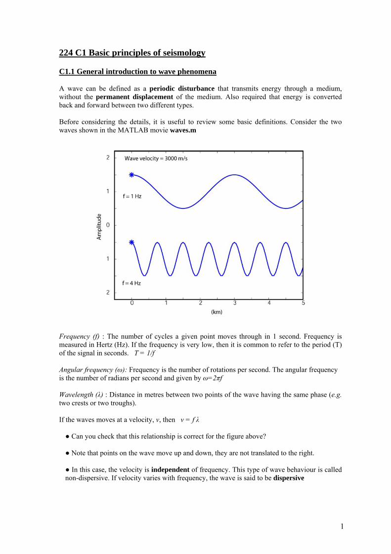
224 C1 Basic principles of seismology C1.1 General introduction to wave phenomena A wave can be defined as a periodic disturbance that transmits energy through a medium, without the permanent displacement of the medium. Also required that energy is converted back and forward between two different types. Before considering the details, it is useful to review some basic definitions. Consider the two waves shown in the MATLAB movie waves.m

Frequency (f) : The number of cycles a given point moves through in 1 second. Frequency is measured in Hertz (Hz). If the frequency is very low, then it is common to refer to the period (T) of the signal in seconds. T = 1/f Angular frequency (ω): Frequency is the number of rotations per second. The angular frequency is the number of radians per second and given by ω=2πf Wavelength (λ) : Distance in metres between two points of the wave having the same phase (e.g. two crests or two troughs). If the waves moves at a velocity, v, then v = f λ ● Can you check that this relationship is correct for the figure above?

● Note that points on the wave move up and down, they are not translated to the right.

● In this case, the velocity is independent of frequency. This type of wave behaviour is called non-dispersive. If velocity varies with frequency, the wave is said to be dispersive

1

In seismology, we need to understand how waves will travel in the Earth. For example, how fast will they go, which direction, how will amplitude vary with distance etc. In general this requires the solution of some complicated differential equations. In Geophysics 224 we will approach this subject through visualization. Wave propagation can be considered in two ways, by considering either wavefronts or rays. These are complementary ways of talking about waves:

Rays denote the direction in which the wave travels. Wavefronts are points on the wave with the same phase (e.g. a line along the crest of a wave is a wavefront). Note that wavefronts and rays are at right angles to each other.

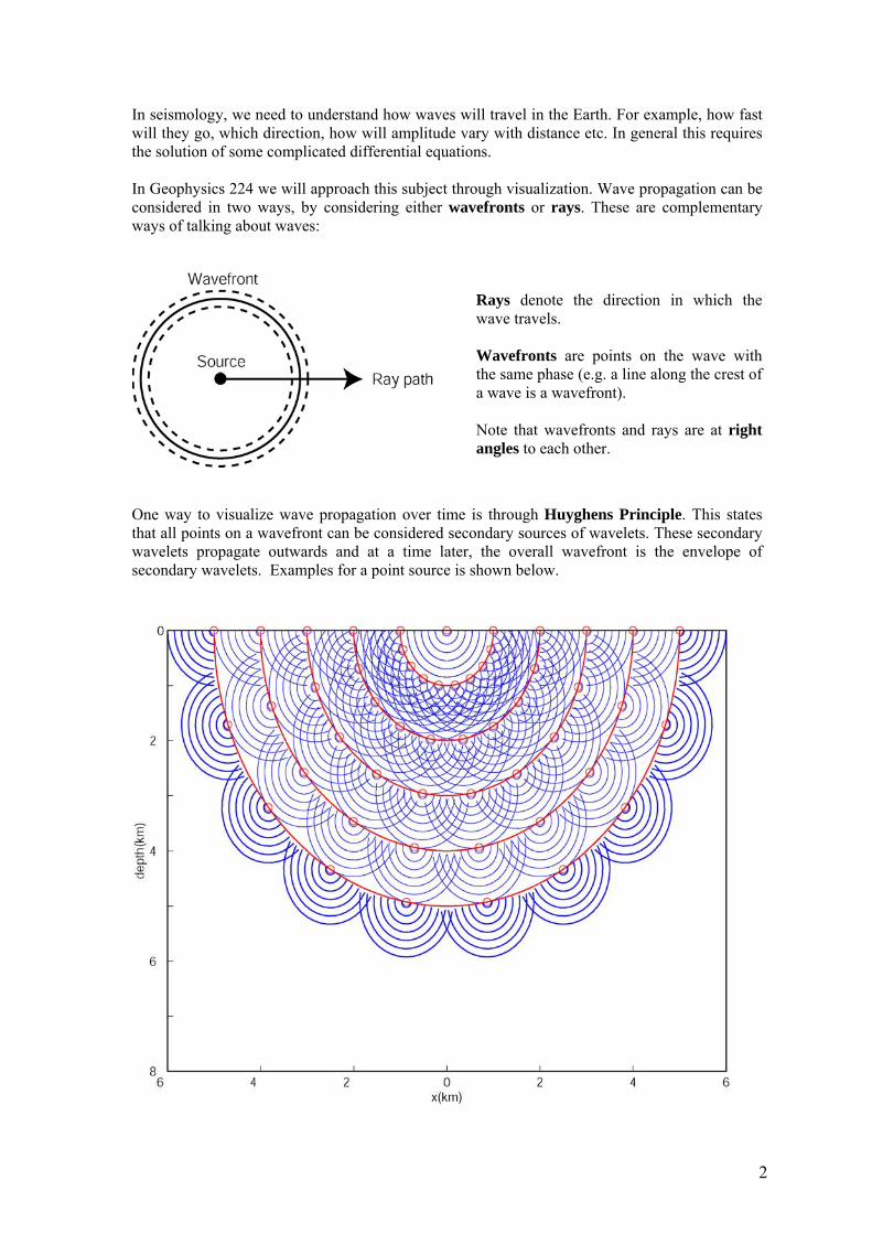
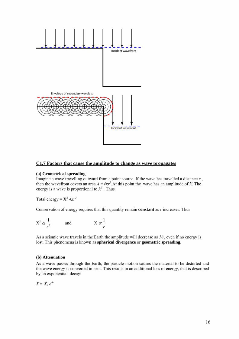
One way to visualize wave propagation over time is through Huyghens Principle. This states that all points on a wavefront can be considered secondary sources of wavelets. These secondary wavelets propagate outwards and at a time later, the overall wavefront is the envelope of secondary wavelets. Examples for a point source is shown below.

2

C1.2 Wave propagation in the Earth Having considered some general aspects of wave propagation we now need to consider how waves will propagate in Earth. Waves in the Earth can be divided into two main categories:

(a) Body waves travel through the bulk medium. (b) Surface waves are confined to interfaces, primarily the Earth-Air interface.

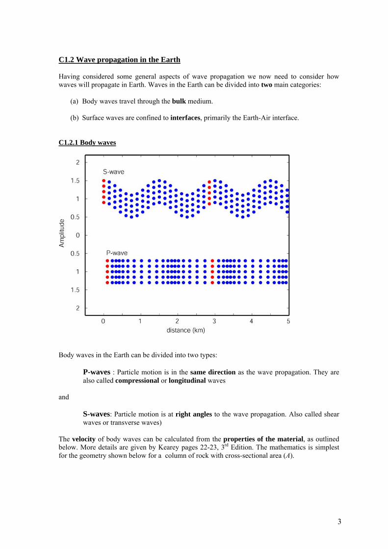
C1.2.1 Body waves

Body waves in the Earth can be divided into two types:

P-waves : Particle motion is in the same direction as the wave propagation. They are also called compressional or longitudinal waves

and

S-waves: Particle motion is at right angles to the wave propagation. Also called shear waves or transverse waves)

The velocity of body waves can be calculated from the properties of the material, as outlined below. More details are given by Kearey pages 22-23, 3rd Edition. The mathematics is simplest for the geometry shown below for a column of rock with cross-sectional area (A).

3

If a force (F) is applied at the left end, this can be considered an applied longitudinal stress = F/A. The rock deforms elastically in response to the applied stress. The deformation of the

leftmost disk can be quantified as the longitudinal strain = LLΔ

The behaviour of the medium is described by the longitudinal modulus, ψ = longitudinal stress / longitudinal strain which is a measure the stiffness of the rock (i.e. how much stress is needed to produce a given strain). This strain produces a force that will cause the shaded section of the rock to accelerate to the right. This lowers the stress to the left, but increases it to the right. This causes the next section of the rock to move and so on. Can show that a wave motion will move down the column at a velocity

ρψ

=v

where ρ is the density of the material. Note that the stiffer the medium (larger ψ) the greater the force on the shaded cylinder, thus acceleration is higher and wave velocity is greater. Similarly, as density increases, the shaded section becomes heavier and it’s acceleration (and wave velocity) for a given force will decrease. In general, the calculation of velocity is more complicated as the deformation will involve both compression and shearing. Two other modulii must be defined to fully understand these effects. Bulk modulus, K = volume stress, P volume strain, ΔV/V and Shear modulus, μ = shear stress, τ shear strain, tan θ

4

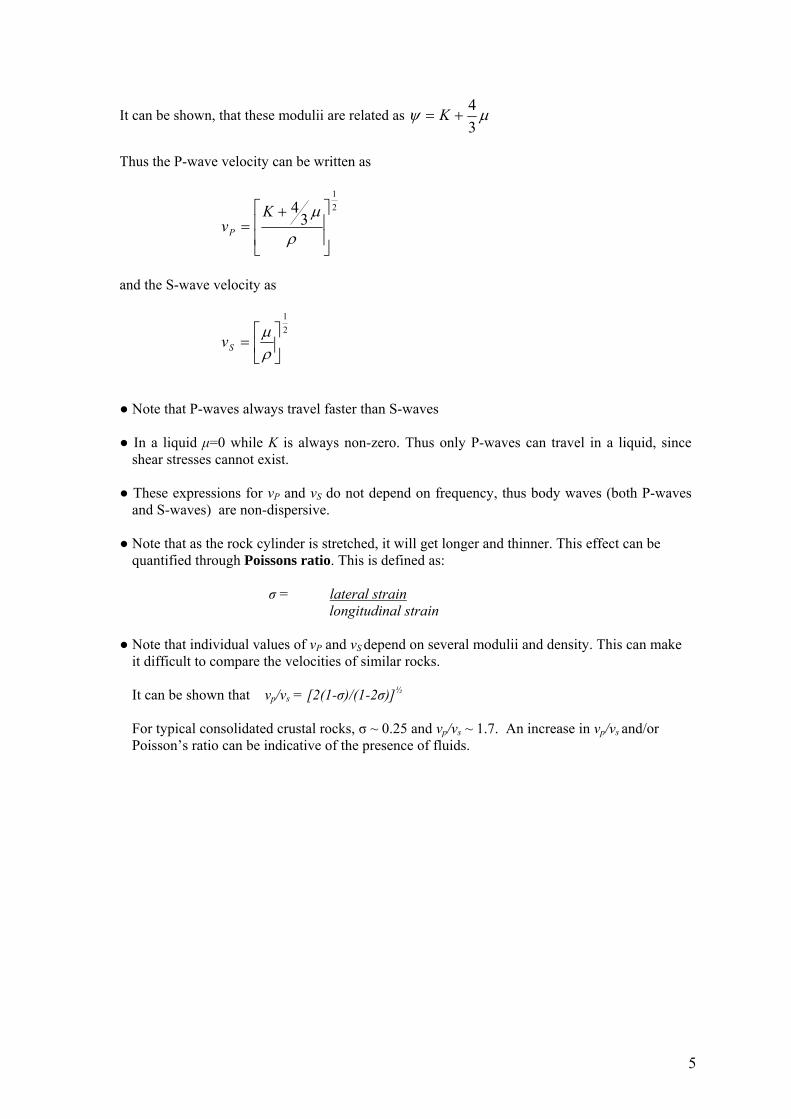
It can be shown, that these modulii are related as μψ34

+= K

Thus the P-wave velocity can be written as

21

34

⎥⎥

⎦

⎤

⎢⎢

⎣

⎡ +=

ρ

μKvP

and the S-wave velocity as

21

⎥⎦

⎤⎢⎣

⎡=

ρμ

Sv

● Note that P-waves always travel faster than S-waves ● In a liquid μ=0 while K is always non-zero. Thus only P-waves can travel in a liquid, since

shear stresses cannot exist. ● These expressions for vP and vS do not depend on frequency, thus body waves (both P-waves

and S-waves) are non-dispersive. ● Note that as the rock cylinder is stretched, it will get longer and thinner. This effect can be

quantified through Poissons ratio. This is defined as: σ = lateral strain longitudinal strain ● Note that individual values of vP and vS depend on several modulii and density. This can make

it difficult to compare the velocities of similar rocks. It can be shown that vp/vs = [2(1-σ)/(1-2σ)]½

For typical consolidated crustal rocks, σ ~ 0.25 and vp/vs ~ 1.7. An increase in vp/vs and/or

Poisson’s ratio can be indicative of the presence of fluids.

5

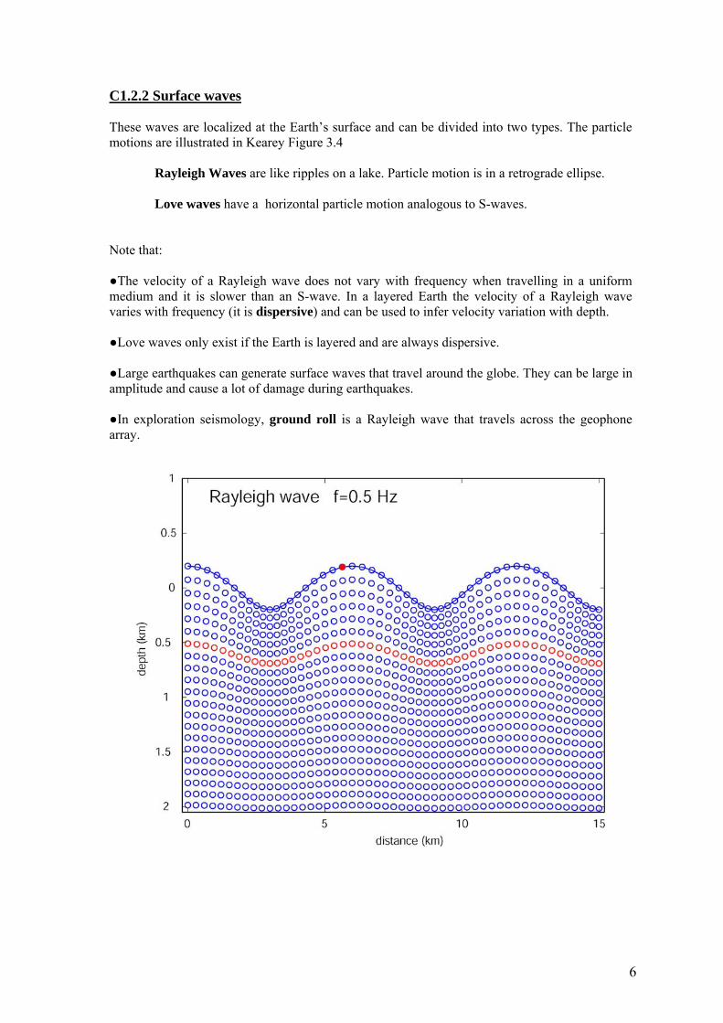
C1.2.2 Surface waves These waves are localized at the Earth’s surface and can be divided into two types. The particle motions are illustrated in Kearey Figure 3.4 Rayleigh Waves are like ripples on a lake. Particle motion is in a retrograde ellipse. Love waves have a horizontal particle motion analogous to S-waves. Note that: ●The velocity of a Rayleigh wave does not vary with frequency when travelling in a uniform medium and it is slower than an S-wave. In a layered Earth the velocity of a Rayleigh wave varies with frequency (it is dispersive) and can be used to infer velocity variation with depth. ●Love waves only exist if the Earth is layered and are always dispersive. ●Large earthquakes can generate surface waves that travel around the globe. They can be large in amplitude and cause a lot of damage during earthquakes. ●In exploration seismology, ground roll is a Rayleigh wave that travels across the geophone array.

6

C1.3 Typical seismic velocities for Earth materials

Typical values for P-wave velocities in km s-1 include:

Sand (dry) 0.2-1.0 Wet sand 1.5-2.0 Clay 1.0-2.5

Tertiary sandstone 2.0-2.5 Cambrian quartzite 5.5-6.0 Cretaceous chalk 2.0-2.5 Carboniferous limestone 5.0-5.5 Salt 4.5-5.0

Granite 5.5-6.0 Gabbro 6.5-7.0 Ultramafics 7.5-8.5

Air 0.3 Water 1.4-1.5 Ice 3.4 Petroleum 1.3-1.4

● why does vp apparently increase with density? e.g. for the sequence granite-ultramafics.

The equation 21

34

⎥⎥

⎦

⎤

⎢⎢

⎣

⎡ +=

ρ

μKvP

suggests that vp should decrease as density increases.

P-wave velocity of porous rocks A rock sample comprises a matrix of rock grains with pores in between. The fractional volume occupied by the pore space is termed the porosity (Φ). Pores are generally filled with a fluid such as air, water, oil or gas. If the matrix has a density ρm and the pore fluid has a density ρf, then the overall density of the rock will be ρ = ρf Φ + (1- Φ) ρm Thus if the velocities in the matrix and fluid are vm and vf it is quite simple to show that

mf vvv)1(1 Φ−

+Φ

=

This equation is sometime called the time-average equation. An example showing how porosity controls vP is in Kearey Figure 3.6. Note that the pore fluid is water, as evidenced by the density at 100% porosity.

7

Example 1 : A rock has 30% porosity and the P-wave velocities in the rock matrix and pore fluid are 1.5 and 2.9 km s-1 respectively. What is the overall seismic velocity? Example 2 : Consider the gas reservoir shown below. The reservoir sand has 10% porosity. The following velocity data was obtained from well-log information

Material vP (km s-1) Sandstone 4.27 Water 1.50 Gas 0.3 Shale 2.4

What is the average P-wave velocity in the water-saturated reservoir? What about in the gas saturated reservoir? Example 3 : In a similar reservoir, the P-wave velocity in the gas filled horizon was measured to be 2.2 km s-1. What porosity does this imply?

Variation of seismic velocity with depth With increasing depth, compaction increase the density of a rock through reduction of pore space. The rigidity of the rock also increases with depth. The net effect is that velocity will increase with depth, even if the lithology does not change.

The increase in velocity with burial depth is quite well defined, and deviations from the expected velocity at a given depth are sometimes used to infer uplift histories in basins. This technique is based on the observation that the compaction is essentially an irreversible process (Telford Figure 4.21)

8

Rippability In geotechnical studies, a knowledge of P-wave velocity can be used to determine if a

particular rock type can be ripped with a given tractor. This also gives a useful

compilation of the range of velocities for a given material. (Kearey Figure 5.25)

As a seismic wave travels through the Earth, several factors will change the direction and amplitude of the waves. When detected at the surface, an understanding of these factors can tell us about sub-surface structure. In sections 1.4 – 1.7 we will examine a number of these factors.

9

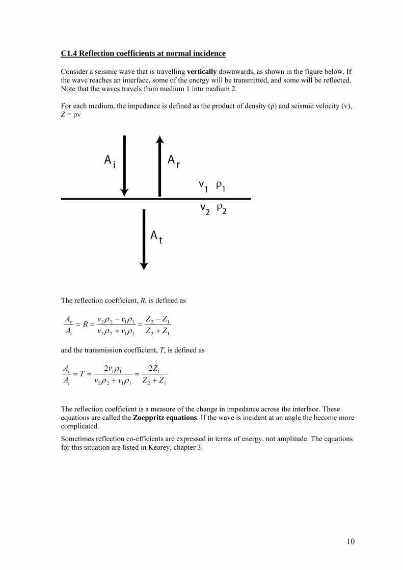
C1.4 Reflection coefficients at normal incidence Consider a seismic wave that is travelling vertically downwards, as shown in the figure below. If the wave reaches an interface, some of the energy will be transmitted, and some will be reflected. Note that the waves travels from medium 1 into medium 2. For each medium, the impedance is defined as the product of density (ρ) and seismic velocity (v), Z = ρv

The reflection coefficient, R, is defined as

12

12

1122

1122

ZZZZ

vvvvR

AA

i

r

+−

=+−

==ρρρρ

and the transmission coefficient, T, is defined as

12

1

1122

11 22ZZ

Zvv

vTAA

i

t

+=

+==

ρρρ

The reflection coefficient is a measure of the change in impedance across the interface. These equations are called the Zoeppritz equations. If the wave is incident at an angle the become more complicated.

Sometimes reflection co-efficients are expressed in terms of energy, not amplitude. The equations for this situation are listed in Kearey, chapter 3.

10

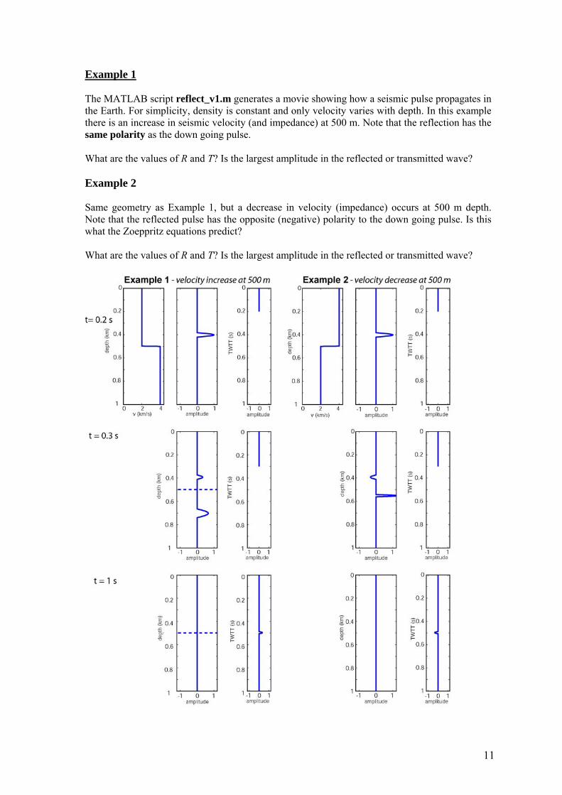
Example 1 The MATLAB script reflect_v1.m generates a movie showing how a seismic pulse propagates in the Earth. For simplicity, density is constant and only velocity varies with depth. In this example there is an increase in seismic velocity (and impedance) at 500 m. Note that the reflection has the same polarity as the down going pulse. What are the values of R and T? Is the largest amplitude in the reflected or transmitted wave? Example 2 Same geometry as Example 1, but a decrease in velocity (impedance) occurs at 500 m depth. Note that the reflected pulse has the opposite (negative) polarity to the down going pulse. Is this what the Zoeppritz equations predict? What are the values of R and T? Is the largest amplitude in the reflected or transmitted wave?

11

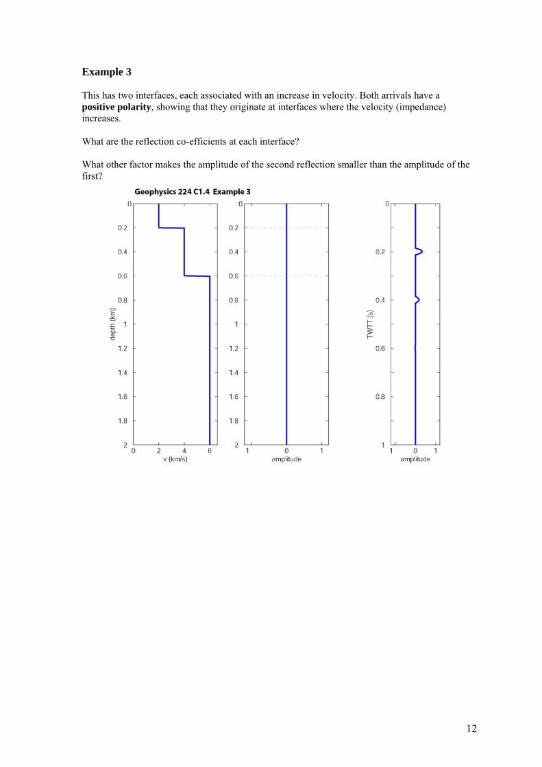
Example 3 This has two interfaces, each associated with an increase in velocity. Both arrivals have a positive polarity, showing that they originate at interfaces where the velocity (impedance) increases. What are the reflection co-efficients at each interface? What other factor makes the amplitude of the second reflection smaller than the amplitude of the first?

12

Example 4 This has a low velocity layer (LVZ). The first reflections has negative polarity show a decrease in velocity, while the second has positive polarity, showing an increase in seismic velocity. Note that a pulse reverberates within the low velocity layer producing multiple later arrivals, with ever decreasing amplitude.

Example 5 Consider a gas reservoir with 10% porosity where the rock matrix has a vp = 3000 ms-1. The overlying rock has vp = 2800 ms-1. ●What is velocity in the reservoir? (use time average equation) ●What value of R is expected for a reflection from the top of the reservoir? ●What value of R is expected where the 2800 ms-1 and 3000 ms-1 layers are in direct contact? This is an example of a bright spot, which is a high amplitude reflection. In the Earth, typical reflection coefficients are ±0.2 with the maximum values ±0.5

13

C1.5 Reflection and refraction at non-normal incidence

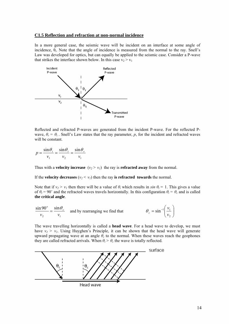
In a more general case, the seismic wave will be incident on an interface at some angle of incidence, θi. Note that the angle of incidence is measured from the normal to the ray. Snell’s Law was developed for optics, but can equally be applied to the seismic case. Consider a P-wave that strikes the interface shown below. In this case v2 > v1

Reflected and refracted P-waves are generated from the incident P-wave. For the reflected P-wave, θr = θi . Snell’s Law states that the ray parameter, p, for the incident and refracted waves will be constant.

121

sinsinsinvvv

p rti θθθ===

Thus with a velocity increase (v2 > v1) the ray is refracted away from the normal. If the velocity decreases (v2 < v1) then the ray is refracted towards the normal. Note that if v2 > v1 then there will be a value of θi which results in sin θt = 1. This gives a value of θt = 90˚ and the refracted waves travels horizontally. In this configuration θi = θc and is called the critical angle.

12

sin90sinvv

co θ= and by rearranging we find that ⎟⎟

⎠

⎞⎜⎜⎝

⎛= −

2

11sinvv

cθ

The wave travelling horizontally is called a head wave. For a head wave to develop, we must have v2 > v1. Using Huyghen’s Principle, it can be shown that the head wave will generate upward propagating wave at an angle θc to the normal. When these waves reach the geophones they are called refracted arrivals. When θi > θc the wave is totally reflected.

14

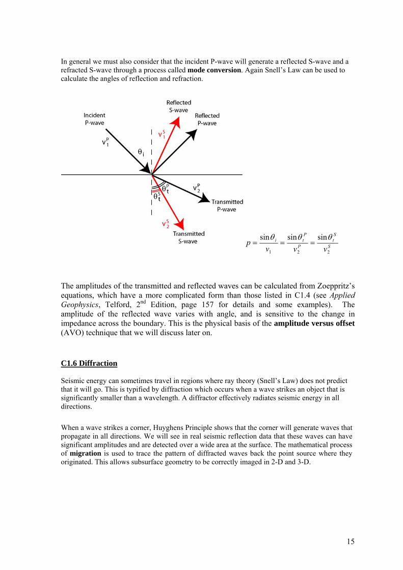
In general we must also consider that the incident P-wave will generate a reflected S-wave and a refracted S-wave through a process called mode conversion. Again Snell’s Law can be used to calculate the angles of reflection and refraction.

S

St

P

Ptip

sinsinsin θθθ===

vvv 221

The amplitudes of the transmitted and reflected waves can be calculated from Zoeppritz’s equations, which have a more complicated form than those listed in C1.4 (see Applied Geophysics, Telford, 2nd Edition, page 157 for details and some examples). The amplitude of the reflected wave varies with angle, and is sensitive to the change in impedance across the boundary. This is the physical basis of the amplitude versus offset (AVO) technique that we will discuss later on. C1.6 Diffraction Seismic energy can sometimes travel in regions where ray theory (Snell’s Law) does not predict that it will go. This is typified by diffraction which occurs when a wave strikes an object that is significantly smaller than a wavelength. A diffractor effectively radiates seismic energy in all directions.

When a wave strikes a corner, Huyghens Principle shows that the corner will generate waves that propagate in all directions. We will see in real seismic reflection data that these waves can have significant amplitudes and are detected over a wide area at the surface. The mathematical process of migration is used to trace the pattern of diffracted waves back the point source where they originated. This allows subsurface geometry to be correctly imaged in 2-D and 3-D.

15

C1.7 Factors that cause the amplitude to change as wave propagates

(a) Geometrical spreading Imagine a wave travelling outward from a point source. If the wave has travelled a distance r , then the wavefront covers an area A =4πr2.At this point the wave has an amplitude of X. The energy is a wave is proportional to X2 . Thus Total energy = X2 4πr2

Conservation of energy requires that this quantity remain constant as r increases. Thus

X2 21r

α and X r1α

As a seismic wave travels in the Earth the amplitude will decrease as 1/r, even if no energy is lost. This phenomena is known as spherical divergence or geometric spreading.

(b) Attenuation As a wave passes through the Earth, the particle motion causes the material to be distorted and the wave energy is converted in heat. This results in an additional loss of energy, that is described by an exponential decay: X = Xo e-kr

16

Where e = 2.718, Xo is the amplitude at r=0 and k is a constant. If k is small, the attenuation will be small, as k increases, the attenuation becomes stronger. In a distance 1/k the amplitude falls

from Xo to Xo e1

.

Another common definition is the absorption coefficient, α, expressed in decibels per wavelength. This is based on the observation that the energy lost is dependent on the number of oscillations per second produced by the wave. Thus high frequencies will attenuation more quickly than low frequencies. This is illustrated in the MATLAB script waves_attenuation.m.

A consequence of frequency-dependent attenuation is that the shape of a pulse can change as it propagates through the Earth. This occurs for the following reasons:

● The pulse can be decomposed into a set of sine or cosine curves with different wavelengths

(Fourier’s Theorem and illustrated in MATLAB script fourier_square_wave.m) ● As the pulse travels the short wavelength signals attenuate more quickly. ● The long wavelengths dominate, giving the pulse a smoother shape and longer duration

(example in Kearey, Figure 3.7)

(c) Scattering Suppose a medium is inhomogeneous and contains some grains with a different seismic velocity to the host rock. Seismic waves will be diffracted / scatteredfrom these grains and energy will be lost from the coherent wavefronts and turned into random seismic energy. The net result is that energy will be lost. Footnote : Decibels A seismic wave changes in amplitude from A1 to A2 as it travels from point 1 to point 2. The corresponding intensity changes from I1 to I2. Note that I1 = A1

2. This change in decibels can be expressed as :

dB = 10 log10 ⎟⎟⎠

⎞⎜⎜⎝

⎛

1

2

II = 20 log10 ⎟⎟

⎠

⎞⎜⎜⎝

⎛

1

2

AA

17

C1.8 Seismic energy sources Basic requirements for an efficient seismic source include: ●Generate sufficient energy in an appropriate frequency band ●Economical ●Non-destructive ●Repeatability 1.8.1 Land seismic sources

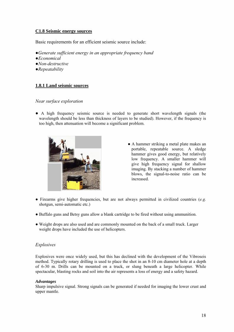
Near surface exploration ● A high frequency seismic source is needed to generate short wavelength signals (the

wavelength should be less than thickness of layers to be studied). However, if the frequency is too high, then attenuation will become a significant problem.

● A hammer striking a metal plate makes an

portable, repeatable source. A sledge hammer gives good energy, but relatively low frequency. A smaller hammer will give high frequency signal for shallow imaging. By stacking a number of hammer blows, the signal-to-noise ratio can be increased.

● Firearms give higher frequencies, but are not always permitted in civilized countries (e.g. shotgun, semi-automatic etc.)

● Buffalo guns and Betsy guns allow a blank cartridge to be fired without using ammunition. ● Weight drops are also used and are commonly mounted on the back of a small truck. Larger

weight drops have included the use of helicopters.

Explosives Explosives were once widely used, but this has declined with the development of the Vibroseis method. Typically rotary drilling is used to place the shot in an 8-10 cm diameter hole at a depth of 6-30 m. Drills can be mounted on a truck, or slung beneath a large helicopter. While spectacular, blasting rocks and soil into the air represents a loss of energy and a safety hazard. Advantages Sharp impulsive signal. Strong signals can be generated if needed for imaging the lower crust and upper mantle.

18

Disadvantages Not repeatable, and quite slow. Most energy is in P-waves (why?). Many environmental concerns and cannot be used in urban areas.

Drilling shot holes in Tibet, 1994 1000 kg shot

Vibroseis

Lithoprobe SNORCLE transect in B.C. Truck generating signal For deeper exploration on land, the Vibroseis method is now the most widely used technique. This does not generate a sharp impulsive signal, but generates a longer waveform that typically lasts 10-20 seconds with frequencies 10-100 Hz.

Data processing requires that the field recording is analysed for correlation with the known source signal. This can allow signal detection in areas with significant seismic noise (e.g. vehicle traffic, wind etc)

Vibroseis trucks can generate forces up to 100,000 N and generally need a hard surface upon which to operate. It is debatable whether they cause no damage to a road. For extra signal strength, multiple trucks are used and they vibrate in phase. Both P-waves and S-waves can be generated.

19

Example 0 : Two separate reflections

Example 1 : Two overlapping reflections

20

Example 2 : Two overlapping reflections and moderate noise levels

Example 3 : Two overlapping reflections and severe noise

21

Stacking is used to increase the signal-to-noise ratio. The inherent assumption of stacking is that the signal is the same each time (coherent) and the noise is different (incoherent). Coherent noise can not be removed by stacking.

22

1.8.2 Marine seismic sources

Air guns An airgun works by releasing a bubble of high pressure air into the water. The rapid expansion of the bubble generates seismic energy with a frequency content around 10-100 Hz.

Operation of Bolt airgun. From Telford ch. 4. The chamber is filled with air at 10-15 MPa which is then released into the water.

Airgun array on Veritas ship

Airgun array and streamers being towed behind a survey vessel.

Advantages ● Very repeatable, reliable source.

Disadvantages

●The bubble pulse oscillates, generating a relatively long wave train. However, by using an array of air guns at differing depths, the combined waveform can be made shorter in duration (figure from Kearey).

● In water only P-waves are generated, but S-waves can be generated by mode conversion at the seafloor.

● In recent years there has been a lot of concern about how marines seismic exploration affects marine mammals.

23

Explosives Once widely used in marine seismics, but now largely replaced by air guns. Bubble pulse problem is difficult to overcome (Kearey figure 3.15), but can be minimized by detonating near the surface (with some loss of energy). Occasionally large shots are used in deep studies but many restrictions are in place to protect oil production facilities and fisheries.

Higher frequency marine sources A range of higher frequency sources are used in marine exploration (100-10000 Hz). These include pingers, sparkers and boomers. The high frequency gives a sharp image of shallow sediment layers, but higher attenuation limits the depth of penetration. These methods are widely used in offshore geotechnical surveying (e.g. choosing locations for seafloor pipes and cables, in harbor construction).

1.8.3 Frequency content of seismic sources Earthquake surface waves 0.1-0.01 Hz Earthquake body waves 10-0.1 Hz Vibroseis 10-100 Hz Air guns 10-100 Hz Explosives 10-300 Hz

24

C1.9 Seismic detectors

C 1.9.1 Onshore seismic exploration

Geophones On land, the surface moves as a P-wave or S-wave arrives. Generally reflected signals arrive at steep angles of incidence. Thus P-waves produce surface motion that is dominantly vertical. Geophones measure ground motion by converting motion into electrical signals. Most geophones measure a single component (vertical), but multiple component ones are sometimes used.

The most common design is the moving-coil geophone. Ensuring good mechanical coupling with the ground is essential, usually through a metal spike. Sometimes a cluster of geophones is planted and the output summed to improve signal to noise ratio. For shallow studies, geophone spacing can be as little as 1 metre. In deeper studies a spacing of 10-50 metres is more usual.

Geophones are manufactured to detect a particular frequency band. This should match the seismic source being used in a particular survey. Geophones are connected to telemetry cables that transmit the recorded signals back to a recording unit.

Seismometers For earthquake studies a more permanent installation is usually required. Three components are usually recorded and the sensor is tuned to detect lower frequencies. Often the seismometer is placed in a shallow vault to minimize wind and other forms of noise.

25

1.9.2 Offshore seismic exploration Hydrophones and streamers S-waves cannot travel in water, so only P-waves can be detected in the water. In marine exploration seismic waves are detected by the change in pressure as a P-wave passes the detector. This type of sensor is called a hydrophone and it converts a change in water pressure into an electric signal through the piezoelectric effect.

In offshore exploration, many hydrophones are placed in neutrally buoyant, oil-filled streamers that can be in excess of 6 km long. The depth is controlled by movable fins and a tail buoy is used to determine the direction of the streamer relative to the ship.

Feathering occurs when ocean currents push the streamer at an angle to the direction in which the survey ship is travelling. Modern ships can pull multiple streamers, and this overcomes feathering and also provides 3-D coverage. Ocean-bottom seismometers (OBS’s) These are like land seismometers, but are dropped to the seafloor from the sea surface. Coupling with the seafloor allows 3 components of motion to be recorded (i.e. P-waves and S-waves can be detected). Generally slow to use, and most widely used in research surveys. Some applications in hydrocarbon exploration.

Dalhousie University OBS on deck Scripps Institution of Oceanography OBS

Geophysics 224 MJU 2006

26