22222222222222222

(MS-WORD MS-POWER POINTAND MS-EXCEL)

SUBMITTED TO

MISSSAPNA VERMA

SUBMITTED BY

AMANDEEP KAUR

CLASS- MBA 1ST D

ROLL NO 120426141

SCHOOL OF MANAGEMENT STUDIES

PUNJABI UNIVERSITY PATIALA

INTRODUCTION

1

MS-Word stands for Micro Soft Word It is Microsofts flagship word processing software It was first released in 1983 under the name Multi-Tool Word for Xenix systems

Microsoft word is a word processing software package We can use it to type letters reports and other document

TO BEGIN WITH MS WORD

Procedure is just simple

Click on start button Click on all programs Find Microsoft office Click on Microsoft office

One another procedure is there for keyboard users

Press window+ R A dialog box is opened named run Type ldquo winwordrdquo

Windows will open MS WORD for different uses like letters newsletters forms etc

GETTING STARTED

TITLE BAR

Title bar displays the name of current document in the centreIf the document is new and is not saved the name of the document is DOCUMENT1 The number suffixed by the word document is depends upon the number of new documents created in a particular sessionThe format of the name displayed in the title bar is the DOCUMENT name- Microsoft Word

The new feature in the title bar is the Quick Access Toolbar to the left corner of the title bar This Quick Access Toolbar includes save and undo buttonwe can use these buttons as quickly as we can

OFFICE BUTTON

2

Right next to the quick access toolbar is the main office button of them all- the office is buttonThis office button similar to what we were used to as the file menu When you click on this office buttonyou can see various file commands

The options like newopensave and others are quite familiarhellip

Next to the menu list we have Recent document list The documents that you have been working with overtime would be displayed under this sectionNext to each document name in the list is a small pin icon which allows you to pin your document permanently to this list in case you donrsquot want the document to disappear from the list when new recent documents get added to this list Just click on this pin and it turns green to indicates that there are sub options for these When you have over your mouse on these options their sub-options will be displayed in the area where previously recent documents were displayed

RIBBON

Ribbon spreads across the screen from left to right and contains all the commands and the difference here is it is context sensitive This means that it is going to change as you work with your document in word For example if you are working with a tablethe ribbon displays the various table commands and tools

3

The ribbon is broken into various tabs like HomeInsertpage layoutreview and view and so on These tabs are organized according to the category of commands If the page lay out tab is selected we can find some groups in it like themespage set-up page background paragraph and arrange All these groups are related to page layout So these are easy to locate like we mentioned earlier the ribbon changes as you work on your document So the home tab is selected we would find a different set of groups like clipboard group font group paragraph group and so on

Each of this group in the tab has some buttons that represent some commands that you may want to use in that group In page layout the page set up group has buttons like margins columns and so on As you have mouse over them we get a small description of what these commands would do

Each of the tabs contains the following tools

Home Clipboard Fonts Paragraph Styles and Editing

Insert Pages Tables Illustrations Links Header amp Footer Text and Symbols

Page Layout Themes Page Setup Page Background Paragraph Arrange

References Table of Contents Footnote Citation amp Bibliography Captions Index and Table of Authorities

Mailings Create Start Mail Merge Write amp Insert Fields Preview Results Finish

Review Proofing Comments Tracking Changes Compare Protect

View Document Views ShowHide Zoom Window Macros

4

WORKING WITH DOCUMENTS

CREATE A NEW DOCUMENT

There are several ways to create new documents open existing documents and save documents in Word

Click the Microsoft Office Button and Click New or

Press CTRL+N (Depress the CTRL key while pressing the ldquoNrdquo) on the keyboard

You will notice that when you click on the Microsoft Office Button and Click New you have many choices about the types of documents you can create If you wish to start from a blank document click Blank If you wish to start from a template you can browse through your choices on the left see the choices on center screen and preview the selection on the right screen

OPENING AN EXISTING DOCUMENT

1048707 Click the Microsoft Office Button and Click Open or

1048707 Press CTRL+O (Depress the CTRL key while pressing the ldquoOrdquo) on the keyboard or

1048707 If you have recently used the document you can click the Microsoft Office Button and click the name of the document in the Recent Documents section of the window Insert picture of recent docs

SAVING A DOCUMENT

5

Click the Microsoft Office Button and Click Save or Save As (remember if yoursquore sending the document to someone who does not have Office 2007 you will need to click the Office Button click Save As and Click Word 97-2003 Document) or

Press CTRL+S (Depress the CTRL key while pressing the ldquoSrdquo) on the keyboard or

Click the File icon on the Quick Access Toolbar

FORMATTING TEXT Styles A style is a format-enhancing tool that includes font typefaces font size effects (bold italics underline etc) colors and more You will notice that on the Home Tab of the Ribbon that you have several areas that will control the style of your document Font Paragraph and Styles

CHANGE FONT TYPEFACE AND SIZE To change the font typeface

1048707 Click the arrow next to the font name and choose a font

6

1048707 Remember that you can preview how the new font will look by highlighting the text and hovering over the new font typeface

To change the font size

1048707 Click the arrow next to the font size and choose the appropriate size or

1048707 Click the increase or decrease font size buttons

Font Styles and Effects Font styles are predefined formatting options that are used to emphasize text They include Bold Italic and Underline To add these to text

1048707 Select the text and click the Font Styles included on the Font Group of the Ribbon or

1048707 Select the text and right click to display the font tools

Font Styles included on the Font Group of the Ribbon or

7


Change Text Color To change the text color

1048707 Select the text and click the Colors button included on the Font Group of the Ribbon or

1048707 Highlight the text right click and choose the colors tool

1048707 Select the color by clicking the down arrow next to the font color button

Highlight Text

Highlighting text allows you to use emphasize text as you would if you had a marker To highlight text

1048707 Select the text

1048707 Click the Highlight Button on the Font Group of the Ribbon or

1048707 Select the text and right click and select the highlight tool

1048707 To change the color of the highlighter click on down arrow next to the highlight button

Copy Formatting If you have already formatted text the way you want it and would like another portion of the document to have the same formatting you can copy the formatting To copy the formatting do the following

1048707 Select the text with the formatting you want to copy

8

1048707 Copy the format of the text selected by clicking the Format Painter button on the Clipboard Group of the Home Tab

1048707 Apply the copied format by selecting the text and clicking on it

FORMATTING PARAGRAPHS

Formatting paragraphs allows you to change the look of the overall document You can access many of the tools of paragraph formatting by clicking the Page Layout Tab of the Ribbon or the Paragraph Group on the Home Tab of the Ribbon

Change Paragraph Alignment

The paragraph alignment allows you to set how you want text to appear To change the alignment

1048707 Click the Home Tab

1048707 Choose the appropriate button for alignment on the Paragraph Group 1048707 Align Left the text is aligned with your left margin

1048707 Center The text is centered within your margins

1048707 Align Right Aligns text with the right margin

1048707 Justify Aligns text to both the left and right margins

9

Indent Paragraphs

Indenting paragraphs allows you set text within a paragraph at different margins There are several options for indenting

1048707 First Line Controls the left boundary for the first line of a paragraph

1048707 Hanging Controls the left boundary of every line in a paragraph except the first one

1048707 Left Controls the left boundary for every line in a paragraph

1048707 Right Controls the right boundary for every line in a paragraph

To indent paragraphs you can do the following

1048707 Click the Indent buttons to control the indent

1048707 Click the Indent button repeated times to increase the size of the indent

1048707 Click the dialog box of the Paragraph Group

1048707 Click the Indents and Spacing Tab

1048707 Select your indents

10

Add Borders and Shading

You can add borders and shading to paragraphs and entire pages To create a border around a paragraph or paragraphs

1048707 Select the area of text where you want the border or shading

1048707 Click the Borders Button on the Paragraph Group on the Home Tab

1048707 Choose the Border and Shading

1048707 Choose the appropriate options

Apply Styles

Styles are a present collection of formatting that you can apply to text To utilize Quick Styles

1048707 Select the text you wish to format

1048707 Click the dialog box next to the Styles Group on the Home Tab

1048707 Click the style you wish to apply

11

Change Spacing Between Paragraphs and Lines You can change the space between lines and paragraphs by doing the following

1048707 Select the paragraph or paragraphs you wish to change

1048707 On the Home Tab Click the Paragraph Dialog Box


1048707 In the Spacing section adjust your spacing accordingly

STYLES

The use of Styles in Word will allow you to quickly format a document with a consistent and professional look Styles can be saved for use in many documents

Apply Styles

There are many styles that are already in Word ready for you to use To view the available styles click the Styles dialog box on the Styles Group in the Home Tab To apply a style


1048707 Click the Styles Dialog Box

1048707 Click the Style you choose

12

ADDING TABLES

Tables are used to display data in a table format Create a Table To create a table

1048707 Place the cursor on the page where you want the new table

1048707 Click the Insert Tab of the Ribbon

1048707 Click the Tables Button on the Tables Group You can create a table one of four ways

1048707 Highlight the number of row and columns

1048707 Click Insert Table and enter the number of rows and columns

1048707 Click the Draw Table create your table by clicking and entering the rows and columns

1048707 Click Quick Tables and choose a table

13

GRAPHICS

Word 2007 allows you to insert special characters symbols pictures illustrations and watermarks

Symbols and Special Characters

Special characters are punctuation spacing or typographical characters that are not generally available on the standard keyboard To insert symbols and special characters

1048707 Place your cursor in the document where you want the symbol

1048707 Click the Insert Tab on the Ribbon

1048707 Click the Symbol button on the Symbols Group

1048707 Choose the appropriate symbol

14

EQUATIONS

Word 2007 also allows you to insert mathematical equations To access the mathematical equations tool



1048707 Click the Equation Button on the Symbols Group

1048707 Choose the appropriate equation and structure or click Insert New Equation

15

Illustrations Pictures and Smart Art Word 2007 allows you to insert illustrations and pictures into a document To insert illustrations

1048707 Place your cursor in the document where you want the illustrationpicture


1048707 Click the Clip Art Button

1048707 The dialog box will open on the screen and you can search for clip art

1048707 Choose the illustration you wish to include

To insert a picture



16

1048707 Click the Picture Button

1048707 Browse to the picture you wish to include

1048707 Click the Picture

1048707 Click Insert

Smart Art is a collection of graphics you can utilize to organize information within your document It includes timelines processes or workflow To insert Smart Art



1048707 Click the Smart Art button

1048707 Click the Smart Art you wish to include in your document

1048707 Click the arrow on the left side of the graphic to insert text or type the text in the graphic

17

WATERMARKS

A watermark is a translucent image that appears behind the primary text in a document To insert a watermark

1048707 Click the Page Layout Tab in the Ribbon

1048707 Click the Watermark Button in the Page Background Group

1048707 Click the Watermark you want for the document or click Custom Watermark and create your own watermark

1048707 To remove a watermark follow the steps above but click Remove Watermark

PAGE FORMATTING

rsquo Modify Page Margins and Orientations The page margins can be modified through the following steps

1048707 Click the Page Layout Tab on the Ribbon

18

1048707 On the Page Setup Group Click Margins

1048707 Click a Default Margin or

1048707 Click Custom Margins and complete the dialog box

Insert Common Header and Footer Information To insert Header and Footer information such as page numbers date or title first decide if you want the information in the header (at the top of the page) or in the Footer (at the bottom of the page) then


1048707 Click Header or Footer

1048707 Choose a style

1048707 The HeaderFooter Design Tab will display on the Ribbon

1048707 Choose the information that you would like to have in the header or footer (date time page numbers etc) or type in the information you would like to have in the header or footer

INSERT A COVER PAGE To insert a cover page

19


1048707 Click the Cover Page Button on the Pages Group

1048707 Choose a style for the cover page

HYPERLINKS

Hyperlinks or links allow the reader to click on text and go to another web site To create a hyperlink

1048707 Select the text that will be the link


1048707 Click the Hyperlink Button on the Links Group

1048707 Type in the web address or URL of the link

1048707 Click OK

20

LISTS

Lists allow you to format and organize text with numbers bullets or in an outline

Bulleted and Numbered Lists

Bulleted lists have bullet points numbered lists have numbers and outline lists combine numbers and letters depending on the organization of the list To add a list to existing text

1048707 Select the text you wish to make a list

1048707 From the Paragraph Group on the Home Tab Click the Bulleted or Numbered Lists button

To create a new list

1048707 Place your cursor where you want the list in the document

1048707 Click the Bulleted or Numbered Lists button

1048707 Begin typing

When you have finished typing and want to exit Word

1 Make sure yoursquove saved the latest version of your document (press ltCtrl sgt)

2 Click on the [Office] button then on the [Exit Word] button (bottom right-hand corner) or you can click on the [x] in the top right-hand corner of the Word window

MAIL MERGE FEATURE

Mail merge is a tool in MS-Word that enables us to create multiple copies of a document with small changes in each In order to create a mail merge two documents are needed a Word Main document and a file with the data or recordsfields

Main document In a mail merge operation the document that contains the text and graphics that remain the same for each version of the merged document for example the return address and body of a form letter

21

Data field A category of information in a data source A data field corresponds to one column of information in the data source The name of each data field is listed in the first row (header row) of the data source PostalCode and LastName are examples of data field names

How to start mail merge-

On the Mailings tab click Start Mail Merge and then click Step by Step Mail Merge Wizard

Select document type

1 In the Mail Merge task pane click Letters This will allow we to send letters to a group of people and personalize the results of the letter that each person receives

2 Click Next Starting document

Select the starting document

1 Click one of the following optionso Use the current document Use the currently open document as our main

documento Start from a template Select one of the ready-to-use mail merge templateso Start from existing document Open an existing document to use as our mail

merge main document2 In the Mail Merge task pane click Next Select recipients

Select recipients

When we open or create a data source by using the Mail Merge Wizard we are telling Word to use a specific set of variable information for our merge Use one of the following methods to attach the main document to the data source

22

Create a database of names and addresses

To create a new database follow these steps

1 In the Mail Merge task pane click Next Select Recipients2 Click Type a new list3 Click Create

The New Address List dialog box appears In this dialog box enter the address information for each record If there is no information for a particular field leave the box blank

By default Word skips blank fields Therefore the merge is not affected if blank entries are in the data form The set of information in each form makes up one data record

4 After we type the information for a record click New Entry to move to the next record

To delete a record click Delete Entry To search for a specific record click Find Entry To customize our list click Customize In the Customize Address List dialog box we can add delete rename and reorder the merge fields

23

5 In the New Address List dialog box click OK In the Save Address List dialog box type the name that we want to give to our data source in the File name box and then click Save

6 In the Mail Merge Recipients dialog box make any changes that we want and then click OK

7 Click Next Write our letter to finish setting up our letter8 Save the main document

When we save the main document at this point we are also saving the data source and attaching the data source to the main document

9 Type the name that we want to give to our main document and then click Save

To proceed to the next step click Next Write our letter

Write our letter

In this step we set up our main document

1 Type or add any text and graphics that we want to include in our letter2 Add the field codes where we want the variable information to appear In the Mail

Merge task pane we have four optionso Address block Use this option to insert a formatted addresso Greeting line Use this option to insert a formatted salutationo Electronic postage Use this option to insert electronic postage

Note This option requires that we have a postage software program installed on our computer

o More items Use this option to insert individual merge fields When we click More Items the Insert Merge Field dialog box appears

Note Make sure that our cursor is where we want to insert the information from our data source before we click More Items

In the Insert Merge Field dialog box click the merge field that we want to use and then click Insert

Note We can insert all of our fields and then go back and add any spaces or punctuation Alternatively we can insert one field at a time close the Insert Merge Fields dialog box add any spaces or punctuation that we want and then repeat this step for each additional merge field that we want to insert We can also format (apply bold or italic formatting to) the merge fields just like regular text

24

3 When we finish editing the main document click Save or Save As on the File menu

Note In Word 2007 click the Microsoft Office Button and then click Save or Save As

Name the file and then click Save To proceed to the next step click Next Preview our letters

Preview our letters

This step allows we to preview our merged data one letter at a time We can also make changes to our recipient list or personalize individual letters

To proceed to the next step click Next Complete the merge

Complete the merge

This step merges the variable information with the form letter We can output the merge result by using either of the following options

Print Select this option to send the merged document directly to the printer We will not be able to view the document on our screen

When we click Print the Merge to Printer dialog box appears In the Merge to Printer dialog box we can choose which records to merge When we click OK the Print dialog box appears Click Print to print the merge document

Edit individual letters Select this option to display the merged document on our screen

When we click Edit individual letters the Merge to New Document dialog box appears In the Merge to New Document dialog box we can choose which records to merge When we click OK the documents are merged to a new Word document

To print the file click the Microsoft Office Button and then click Print

25

SOME SHORT KEYS OF MS-WORD 1 Shift + arrows = for selection2 Ctrl+ 2 = double spacing3 Ctrl+ N = new blank documents4 Ctrl+ O = open5 Ctrl+ S = save6 Ctrl+ P = print the document7 Ctrl + Z = undo8 Ctrl+ Y = repeat the last command9 Ctrl+ C = copy the selected text10 Ctrl+ x = cut the selected text11 Ctrl+ V = paste the selected text12 Ctrl+ F = find13 Ctrl+ shift+ F = types of font14 Ctrl+ shift+ P = font size change15 Shift+F3 = change the case16 Ctrl+ B = bold17 Ctrl+ I = Italian18 Ctrl+ U = underline19 Ctrl+ L = alignment left20 Ctrl+ J = justified alignment21 Ctrl+ E = centre alignment22 Ctrl+ R = alignment right23 Ctrl+ H = replace alignment24 Alt+ tab = document move from one to another25 Alt+F4 = to close the document or exit26 F1 = help27 F7 = to check grammar28 F12 = save as29 Ctrl+ shift+lt = decrease font size30 Ctrl+ shift+gt = increase font size31 Ctrl+[ = increase font size by one point32 Ctrl+] = decrease font size by one point33 Right arrows = move by one cursor34 Ctrl+ right+ arrow = move by one word35 Page up = above36 Page down = below37 Home = go to top38 End = end of the document

26

Power Point 2007

Getting Started with Power Point 2007 class will show whatrsquos different in Power Point 2007 and whatrsquos the same The Ribbon at the top of the page has replaced menus and toolbars in Word Excel PowerPoint Access and new messages in Outlook This class will cover the use of the Ribbon the Office Button (where is the File menu) getting Help and online Training Live Preview the Mini Toolbar the Quick Access Toolbar new File Formats and a Few Fun Features The class and short handout are designed so when you return to your office you can begin using Power Point 2007

There are three major differences in Power Point 2007 the Ribbon the MS Office Button and the new file formats

The Ribbon

The Ribbon at the top of the page has replaced menus and toolbars in Word Excel PowerPoint Access and new messages in Outlook

Tabs ndash Represent core tasksGroups ndash Are sets of related commandsCommands ndash Are buttons menus or boxes where you enter information

Home Tab

Try it

1 Start PowerPoint 20072 Click on each tab to display different

groups of commands3 Mouse-over a command for

Enhanced Toolbar Tips Note keyboard shortcuts are shown if available

27

The Home Tab displays the most commonly used commands In PowerPoint Word and Excel these include Copy Cut and Paste Bold Italic Underscore etc The commands are arranged in groups Clipboard Font Paragraph Styles and Editing

The most frequently used commands Paste Cut and Copy are the left most in the first group in the Home Tab

Insert Tab Insert tables pictures diagrams charts text boxes sounds hyperlinks headers and footers

Design Tab Select background design fonts and color scheme

Animations Tab Select animating effects

Slide Show Tab Select starting slide record narration and more

Review Tab Spelling research and more

View Tab Change the view to the notes page or normal Turn on gridlines

The less frequently used commands or command choices can be displayed by clicking the down arrow under the command

Try it

1 Copy some text2 On the Home Tab in the

Clipboard Group click the down arrow under Paste to display the Paste Special Command

Contextual Tabs (On Demand)

Some commands only appear when you need them For example The Drawing Tools Tab only appears when you select text or drawings

Try it

1 Select some text2 Click the Format tab3 Click a different slide and the

Format tab disappears

28

Galleries (with Table Tools example)

Galleries are collections of thumbnail graphics They give you quick visual access to available formats

Try it

1 On the Format tab click the More arrow in the Shape Styles group

2 Mouse-over the graphics presented to see the shape styles change

Live Preview (with Animations Example)

Live Preview temporarily applies formatting on the selected text or object when you mouse-over any of the formatting buttons This allows you to preview how the text or object would appear without having to apply the formatting

Try it

1 Select some text2 Click the Drawing Tools

Format Tab3 Click Quick Styles and mouse-

over the gallery selections for a Live Preview

Insert SmartArt

SmartArt can be inserted from the Insert tab gt SmartArt or by selecting a new slide that contains

content placeholders or by selecting a bulleted list and selecting the Convert to SmartArt

Graphic button on the Home tab

Try it

1 Click the Home tab2 Click New Slide3 Select a slide that contains

content placeholders4 Click the Insert SmartArt

placeholder5 Select the desired graphic or6 Select a bulleted list7 Select the Convert to

SmartArt Graphic button on the Home tab

Dialog Box Launcher

The Dialog Box Launcher at the bottom of any group displays more options

Try it

1 Click the arrow at the bottom of font group to view more options or commands

ShowHide Groups

When the screen is lower resolution or the program window is small some groups may display only the group name Click the down arrow

Try it

1 Make the program window smaller until some groups only show the group name

2 Click the down arrow under a group name

29

under the group name to see the commands for that group

Minimize the Ribbon

To minimize the Ribbon right click in the tab area or right click on any command

Try it

1 Right click in the tab area2 Select Minimize the Ribbon3 Right click in the tab area4 De-select Minimize the

Ribbon

Mini Toolbar

The Mini Toolbar pops up whenever text is selected to provide easy access to the most commonly used formatting commands The toolbar will also appear when you right-click on a selection of text (Note You do not have the ability to customize the Mini toolbar)

Try it

1 Select some text2 Mouse over the

selected text and upwards

3 Click any of the formatting commands on the Mini Toolbar

Right-Click

Right-click to find many more commands Try it

1 Select some text2 Right-click on the selected text

30

The Office Button (Top Left Corner)

The Office Button has replaced the File menu It contains the commands for handing files such as New Open Save Save As and Print and file preparation commands such as Prepare gt Properties exit the application and Recent Documents

Try it

1 Mouse-over the Office Button to see its functions

2 Click the Office Button3 Mouse-over the commands on

the left for an explanation of each command

4 Click the push pin in the Recent Documents keep a document on the list

The Options Button

The Options Button at the bottom of the Office Button menu allows you to change your preferences

Try it

1 Click the Office Button2 Click the Options Button3 Click on each of the selections listed on the

right4 Click Save to customize where your files are

saved or change the default file format5 Click Proofing gt AutoCorrect Optionshellip to

change how Word corrects text as you type

Quick Access Toolbar (Top Left Right of Office Button)

The Quick Access Toolbar is a customizable toolbar which contains shortcuts for commonly

used commands You can either click the down arrow to add or remove commands or right click on any command to add that command to the toolbar

Try it

1 Right-click any command and click Add to Quick Access Toolbar

2 Click the More button on the Quick Access Toolbar

3 Click any of the displayed commands to add them to the toolbar or click More Commands


5 Right-click any command on the Quick Access Toolbar and click Remove from Quick Access Toolbar

31

Help (Upper Right Corner) or F1

The Help Menu is now organized by topic You can also use the Search box

Try it

1 Click Help gt Whatrsquos new2 Click Help gt Training3 Click Help Enter some text in the

Search box

New File Formats - OpenXML

PowerPoint Word and Excel now offer new file formats based on Office Open XML (Extensible Markup Language) formatsOpen XML files

Reduce file size by up to 75 Improve security and reliability Are the old extension followed by an ldquoxrdquo or ldquomrdquo

Exampleso pptx for PowerPoint presentations

Access has a new file format accdb

PowerPoint Word Excel and Access 2007 are able to open files from previous versions By default new files are saved in the new formats and old files are saved in the old formats (exception PowerPoint 95)

When you save a file in the old format a Compatibility Checker is run It will alert you to any features that are not compatible with the old version

Users running Word Excel and PowerPoint 2000-2003 can open the new file types after they download a converter

ITS recommends saving your files as Word 97 ndash 2003 Documents Excel 97 ndash 2003 Worksheets or PowerPoint 97 ndash 2003 Presentations Doing so ensures that users who have not upgraded to Office 2007 will still be able to open and edit the files

Click Office Button gt PowerPoint Options gt Save gt Save files in this format to change the default save format

Try it

1 Open a PowerPoint 2003 Presentation

2 Note the Title Bar shows ldquoCompatibility Moderdquo

3 Click the Office Button4 Select Prepare gt Run

Compatibility Checker gt OK

5 Click the Office Button6 Select Save As gt

PowerPoint Presentation

7 Note the filetype is PowerPoint Presentation (and may show pptx)

8 Select the Cancel Button


PowerPoint 97-2003 Presentation

11 Note the filetype is PowerPoint 97-2003 (and may show ppt)


13 Click the Office Button gt PowerPoint Options gt Save gt Save files in this format if you want to change the default save format

32

A Few More Fun Features (as time permits)

Save as PDF

You can download an add-on for no-charge that allows you to save files in PDF format

Try it

1 Click the Office Button2 Select Save As gt Find add-ins

for other file formats

Zoom Slider (lower right corner)

You can easily zoom in and out in Word Excel and PowerPoint using the zoom slider

Try it

1 Click the slider and move it left and right

Keyboard Shortcuts

New keyboard shorts cuts called KeyTips are available using the Alt key The ldquooldrdquo shortcuts that start with CTRL like CTRL-C for copy also still work

Try it

1 Select some text2 Press the Alt key3 Type the displayed number 1 to

bold the selected text4 Type the displayed letter H to

select the Home Tab5 Press Alt again to toggle off the

KeyTips

Online Training and Other ResourcesVisit Office 2007 Training and Other Resources athttpcsitsuiowaedusdaoffice2007trainingshtml for a wealth of help including

The schedule of Office 2007 classes being offered The ITS Help Desk Hawkmail Support Documentation Microsoft Interactive Guides The Life After Guideshellip How-to manuals for Word Outlook and Outlook Web Access Microsoft E-Learning online classes SkillSoft online classes Microsoft Online Training especially the online Demos of the Office Products

33

Letrsquos Get Started

Open an Existing Presentation Office Button

1 Click the Office button and select Open2 Navigate to the existing document you wish to open3 Once you have selected your document click the Open button

Start a Slide Show Slide Show Tab

1 Click the Slide Show tab

2 Click From Beginning or From Current Slide

Create a New Presentation Office Button

1 Click the Office button and select New2 Select a Blank Presentation or a Recently Used Template3 Click the Create button in the lower right corner

Choose a Theme (Sets of Colors Fonts Effects and Background Styles)Design Tab

1 Click the Design tab2 Mouse-over the design gallery and select a theme

Insert a New Slide and Add Content Home Tab

1 Click the Home tab

2 Click New Slide

3 Select a slide that contains content placeholders 4 Mouse- over and select a place holder to insert a Table Chart SmartArt Graphic

Picture Clip Art or Media Clip5 Or type text

34

Insert and Format a Picture Using the Content Placeholders Home amp Picture Tabs

1 Select the Picture content placeholder on a new slide2 Navigate to the location where your picture is located3 Double-click the picture you want to insert4 Select the picture you inserted and the Picture Tools tab appears5 On the Picture Tools tab click the Format button Mouse-over the Picture Styles

Gallery for live preview

Insert a Picture Using the Insert Tab Insert Tab1 Select any slide2 Click an insertion point within that slide3 Click the Insert tab4 Click Picture5 Navigate to the location where your picture is located6 Double-click the picture you want to insert7 Select the picture you inserted and the Picture Tools tab appears8 Click and drag the Picture to desired location on the slide

Insert a Text Box Insert Tab

1 Select any slide2 Click the Insert tab3 Click Text Box4 Click and drag within the slide to draw the text box5 Click in the text box6 On the Format tab mouse- over and select a shape style

Insert an Organizational Chart Insert Tab or Content Holder

1 Either click on Insert gt SmartArt gt the Org Chart graphic or select the SmartArt content holder on a slide

Convert an Existing Bulleted List to a Graphic Home Tab

1 Select a bulleted list on a slide

2 On the Home tab click the Convert to SmartArt Graphic button 3 Mouse-over the selections offered or click More SmartArt Graphics

Easily Edit the SmartArt Text1 Click on some text in a SmartArt Graphic

35

INTRODUCTION TO MS EXCEL

Microsoft Excel is one of the most popular spreadsheet applications that helps you manage data

create visually persuasive charts and thought‐provoking graphs Excel is supported by both Mac

and PC platforms Microsoft Excel can also be used to balance a checkbook create an expense

report build formulas and edit them

HOW TO LAUNCH MS EXCEL

To begin Microsoft Excel

Click on start button

Go to all programs

Find applications

Click on Microsoft office

Click on MD EXCEL

When opened a new spreadsheet will pop up

36

SAVING A DOCUMENT

Before you begin you should save your document To do this click on the floppy disk

located at the top of the screen Then Microsoft Excel will open a dialog box where you can

specify the new filersquos name location of where you want it saved and format of the document

Once you have specified a name place and format for your new file press the Save button

37

SAVING LATER

After you have initially saved your blank document under a new name you can begin your

project However you will still want to periodically save your work as insurance against a

computer freeze or a power outage To save just click on the floppy disk or for a shortcut press

CTRL + S

TOOLBARS

In Microsoft Excel 2007 for a PC the toolbars are automatically placed as tabs at the top of the

screen Within these tabs you will find all of your options to change text data page layout and

more To be able access all of the certain toolbars you need to click on a certain tab that is

located towards the top of the screen

THREE COMMONLY USED TABS

The Home Tab This is one of the most common tabs used in Excel You are able to format the

text in your document cut copy and paste informationChange the alignment of your data

38

insert delete and format cells The HOME TAB also allows you to change the number of your

data (ie currency time date)

HOME TAB

The Insert Tab This tab is mainly used for inserting visuals and graphics into your document

There are various different things that can be inserted from this tab such as pictures clip art

charts links headers and footers and word art

The Page Layout Tab Here you are able to add margins themes to your document change the

orientation page breaks and titles The scale fit of your document is also included as a feature

within this tab if needed

39

FORMATTING

WORKING WITH CELLS

Cells are an important part of any project being used in Microsoft Excel Cells hold all of the

data that is being used to create the spreadsheet or workbook To enter data into a cell you

simply click once inside of the desired cell a black border will appear around the cell This

border indicates that it is a selected cell You may then begin typing in the data for that cell

CHANGING AN ENTRY WITHIN A CELL

You may change an entry within a cell two different ways

10487071048707Click the cell one time and begin typing The new information will replace any information

that was previously entered

10487071048707Double click the cell and a cursor will appear inside This allows you to edit certain pieces of

information within the cells instead of replacing all of the data

CUT COPY AND PASTE

You can use the Cut Copy and Paste features of Excel to change the data within your

spreadsheet to move data from other spreadsheets into new spreadsheets and to save yourself

the time of re‐entering information in a spreadsheet

Cut will actually remove the selection from the original location and allow it to be placed

somewhere else

Copy allows you to leave the original selection where it is and insert a copy elsewhere

Paste is used to insert data that has been cut or copied

40

To Cut or Copy

Highlight the data or text by selecting the cells that they are held within

Go to the Home Tab gt Copy (CTRL + C) or Home Tab gt Cut (CTRL + X)

Click the location where the information should be placed

Go to Home Tab gt Paste (CTRL + V) to be able to paste your information

FORMATTING CELLS

There are various different options that can be changed to format the spreadsheets cells

differently When changing the format within cells you must select the cells that you wish to

format

To get to the Format Cells dialog box select the cells you wish to change then go to Home Tab

gt Format gt Format Cells A box will appear on the screen with six different tab options

Explanations of the basic options in the format dialog box are bulleted below

41

Number Allows you to change the measurement in which your data is used (If your data is

concerned with money the number that you would use is currency)

Alignment This allows you to change the horizontal and vertical alignment of your text within

each cell You can also change the orientation of the text within the cells and the control of the

text within the cells as well

Font Gives the option to change the size style color and effects

Border Gives the option to change the design of the border around or through the cells

FORMATTING ROWS AND COLUMNS

When formatting rows and columns you can change the height choose for your information to

autofit to the cells hide information within a row or column un‐hide the information To format

a row or column go to Home Tab gt Row Height (or Column Height) then choose which height

you are going to use The cell or cells that are going to be formatted need to be selected before

doing this When changing the row or column visibility (hidden un‐hidden) or autofit you will

go to the Home Tab and click Format The drop down menu will show these options

42

ADDING ROWS AND COLUMNS

When adding a row or column you are inserting a blank row or column next to your already

entered data Before you can add a Row you are going to have to select the row that you wish for

your new row to be placed (Rows are on the left hand side of the spreadsheet) once the row is

selected it is going to highlight the entire row that you chose To insert the row you have to go to

Home Tab gt Insert gt Insert Sheet Rows The row will automatically be placed on the

spreadsheet and any data that was selected in the original row will be moved down below the

new row

Before you can add a Column you are going to have to select a column on the spreadsheet that is

located in the area that you want to enter the new column (Columns are on the top part of the

spreadsheet) Once the column is selected it is going to highlight the entire row that you chose

To insert a column you have to go to Home Tab gt Insert gt Insert Sheet Column (Figure 11)

The column will automatically be place on the spreadsheet and any data to the right of the new

column will be moved more to the right

43

WORKING WITH CHARTS

Charts are an important part to being able to create a visual for spreadsheet data In order to

create a chart within Excel the data that is going to be used for it needs to be entered already into

the spreadsheet document Once the data is entered the cells that are going to be used for the

chart need to be highlighted so that the software knows what to include Next click on the Insert

Tab that is located at the top of the screen

You may choose the chart that is desired by clicking the category of the chart you will use Once

the category is chosen the charts will appear as small graphics within a drop down menu To

choose a particular chart just click on its icon and it will be placed within the spreadsheet you are

working on To move the chart to a page of its own select the border of the chart and Right

Click This will bring up a drop down menu navigate to the option that says Move Chart This

will bring up a dialog box that says Chart Location From here you will need to select the circle

next to As A New Sheet and name the sheet that will hold your chart The chart will pop up

larger in a separate sheet but in the same workbook as your entereddata

44

CHART DESIGNS

There are various different features that you can change to make your chart more appealing To

be able to make these changes you will need to have the chart selected or be viewing the chart

page that is within your workbook Once you have done that the Design Tab will appear

highlighted with various different options to format your graphic

45

CHART OPTIONS

Titles To add titles to a chart of graphic you have to click on the Insert Tab Once you have

done this click on the Text Box Icon This will insert a text box that you can type the title and

place anywhere you wish on the chart Change Chart Type You can change your chart easily

by selecting this icon and navigating to a more desirable chart This feature is very convenient

for someone who chose the wrong chart and doesnrsquot wish to reselect all their data and go through

the process a second time

Format Chart Area This allows for changes to be made to the chards border style fill

shadows and more To get this option you will need to right click on the charts border and

navigate to the Format Chart Area option Once this is clicked a dialog box will appear

CHART STYLE

Here you are able to change the color of the bars that are within your chart

CREATING FUNCTIONS

When creating a function in Excel you must first have the data that you wish to perform the

function with selected

10487071048707Select the cell that you wish for the calculation to be entered in (ie if I want to know the

sum of B1B5 I will highlight cell B6 for my sum to be entered into)

10487071048707Once you have done this you will need to select the Formulas Tab located at

the top of the screen

10487071048707A list of Most Recently Used Financial Logical Text Date and Time Math and Trig

formulas will appear To choose one of the formulas click the icon that holds the formula you are

looking for

10487071048707Once you have clicked your formula this will display a dialog box on your screen

46

In this screen it lists the cells that are being calculated the values within the cells and the end

result

10487071048707To accept that calculation you can press OK and the result will show up in the selected cell

Basic functions

Some of the most commonly used functions include

SUM() to calculate the total of a set of numbers

AVERAGE() to calculate the average of a set of numbers

MAX() to calculate the maximum value within a set of numbers

MIN() to calculate the minimum value within a set of numbers

ROUND() to round a set a values to a specified number of decimal places

TODAY () to show the current date

IF() to calculate a result depending on one or more conditions

So how do you use a function

A function makes use of values or cell references just like a simple formula does The numbers

or cell references that it needs for its calculations are placed in brackets after the name of the

function

47

The formula is equivalent to the function

= 12 + 195 + 67 ndash 43 = SUM(12 195 67 -43)

= (B3 + B4 + B5 + B6) =SUM(B3B6)

= (B3 + B4 + B5 + B6)4 = AVERAGE (B3B6)

Several popular functions are available to you directly from the Home ribbon

1 Select the cell where you want the result of the calculation to be displayed

2 Click the drop-down arrow next to the Sum button

3 Click on the function that you want

4 Confirm the range of cells that the function should use in its calculation (Excel will try

to guess this for you If you donrsquot like what it shows inside the dotted line then click and drag

to make your own selection)

As an example to calculate the average for the following set of tutorial results you would

1 Click on cell F3 to make it active

2 Click on the arrow next to the Sum button and select Average

3 Press [ENTER] to accept the range of cells that is suggested (B3E3)

Thatrsquos it You can now copy the formula in cell F3 down to cells F4 and F5 ndash using relative

addressing because you want a different set of tutorial marks to be used for each student

If you want to use a function that isnrsquot directly available from the drop-down list then you can

click on More Functions to open the Insert Function dialog box Another way to open this

dialog box is to click the Insert Function icon on the immediate left of the formula bar

The Insert Function dialog box displays a list of functions within a selected function category If

you select a function it will briefly describe the purpose and structure of the function

When you click the OK button at the bottom of the window yoursquoll be taken to a

second dialogue box that helps you to select the function arguments (usually the

range of cells that the function should use)

48

Some functions use more than one argument For example the ROUND() function

needs to know not only which cells to use but also how many decimal places those

cells should be rounded to So the expression =ROUND(G5G8 0) will round the

values in cells G5 to G8 to the nearest whole number (ie no decimal places)

Note that the ROUND() function actually changes the value that is stored in your

worksheet based on the arguments yoursquove provided Formatting options such as

Currency or Increase Decrease Decimal simply change the appearance of a number

but all its decimal places are still kept and displayed in the formula bar

The IF() function

The IF() function is getting a section all of its own because for many people itrsquos

not as intuitive to understand as the common maths and stats functions

The IF() function checks for a specific condition If the condition is met then one

action is taken if the condition is not met then a different action is taken For

example you may be reviewing a set of tutorial marks If a studentrsquos average mark is

below 50 then the cell value should be FAIL so the condition you are checking is

whether or not the average result is below 50 If this condition is not met (that is the

average result is 50 or more) then the cell value should be PASS

Letrsquos see this in action

The structure of an IF() function is

=IF (condition result if true result if false)

Using English to describe our example as an IF statement IF the average mark is less

than

50 then display the word ldquoFAILrdquo else display the word ldquoPASSrdquo

Now for a real work sheet example Look at the formula bar in the screenshot below

Do you follow how the formula in cell G4 was constructed Because the average mark is stored

in cell F4 we need to check whether the value in F4 is less than 50 If it is then the active cell

49

(G4) must display the word ldquoFailrdquo If the value in F4 is not less than 50 then the active cell

must display the word ldquoPassrdquo Thatrsquos not really so complicated is it

Nested functions

Take a deep breath and donrsquot panic I just want to show you that if you need to you can include

one function inside another

In the example above we first worked

out the Average mark and then the PassFail outcome But we could have done it all in

a single step by using the following formula in row 3

=IF(AVERAGE(B3E3) lt 50 ldquoFAILrdquo ldquoPASSrdquo)

In this IF statement Irsquove nested one function inside another The reference to cell F4 has been

replaced with a function that calculates the average tutorial mark and then checks it against the

same condition as before (ldquolt 50rdquo) with the same possible outcomes Doing it this way you

wouldnrsquot need column F in the worksheet at all

Of course in real life yoursquod expect to get students coming to query their PassFail

status and would probably want to keep the Average column to explain the outcome

thatrsquos been allocated to them So the first example using a separate Average and

Outcome is not only simpler itrsquos also more practical

WORKING WITH MACROS

A macro is a shortcut for performing a series of actions in an Excel worksheet Macros are useful

for automating complex or repetitive tasks especially if the work is being shared because it is

easier to explain one step (ie activate the macro) than it is to explain several steps Once a

macro is created you can activate it by using the Macro dialog box or by pressing a keyboard

combination

50

CREATING amp RECORDING A NEW MACRO

1 From the Developer command tab in the Code group click RECORD MACRO

The Record Macro dialog box appears

2 In the Macro name text box type a name for the new macro A macro name must begin with a

letter and contain no spaces or special characters Underscores ( _ ) are permissible

3 OPTIONAL In the Shortcut key text box type a letter that will be used to activate the macro

4 To save the macro to the workbook that is currently open from the Store macro in pull-down

list select This Workbook To save the macro to a new workbook from the Store macro in pull-

down list select New Workbook To save the macro to Excel for use in any workbook from the

Store macro in pull-down list select Personal Macro Workbook

5 OPTIONAL In the Description text box type a summary of the macros function or any other

information

6 Click OK The Record Macro dialog box closes and the macro begins recording

7 Perform the exact series of commands you want the macro to accomplish

8 When finished from the Developer command tab in the Code group click

STOP RECORDING

The recording stops and the macro is saved

Running a Macro You can run a macro only after it has been created and recorded Once you

have chosen to run a macro the macro will complete its commands until finished or until you

suspend the macro

51

WARNING You should save your workbook before running a macro If the macros

results are undesirable you can close the workbook without saving and then reopen it

preserving the state of your workbook before using the macro

Running a Macro Ribbon Option

1 OPTIONAL If the insertion point is critical set it in the appropriate location

NOTE This step will be useful if the macros commands require you to begin in a specific cell

2 From the Developer command tab in the Code group click MACROS The Macro dialog box

appears

3 From the Macro name scroll box select the macro you want to run

4 Click RUN

The Macro dialog box closes and the selected macro performs the steps it Recorded

Deleting a Macro

If you no longer need a macro you can delete it Once a macro has been deleted it is no longer

available in any workbook however changes that have already been made by the macro will not

be undone

1 From the Developer command tab in the Code group click MACROS The Macro

dialog box appears

2 From the Macro name scroll box select the macro you want to delete Click DELETE

3 A confirmation dialog box appears

4 To confirm the deletion click YES

5 To delete more macros repeat steps 1ndash4

6 The macro is deleted and the Macro dialog box closes

52

53



Select recipients


Write our letter

Preview our letters

Complete the merge

Power Point 2007

The Ribbon

Home Tab




Insert SmartArt

Dialog Box Launcher

ShowHide Groups

Minimize the Ribbon

Mini Toolbar

Right-Click


The Options Button





Online Training and Other Resources





Choose a Theme (Sets of Colors Fonts Effects and Background Styles) Design Tab



Insert a Picture Using the Insert Tab Insert Tab




Easily Edit the SmartArt Text

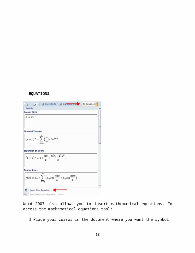
MS-Word stands for Micro Soft Word It is Microsofts flagship word processing software It was first released in 1983 under the name Multi-Tool Word for Xenix systems

Microsoft word is a word processing software package We can use it to type letters reports and other document

TO BEGIN WITH MS WORD

Procedure is just simple

Click on start button Click on all programs Find Microsoft office Click on Microsoft office

One another procedure is there for keyboard users

Press window+ R A dialog box is opened named run Type ldquo winwordrdquo

Windows will open MS WORD for different uses like letters newsletters forms etc

GETTING STARTED

TITLE BAR

Title bar displays the name of current document in the centreIf the document is new and is not saved the name of the document is DOCUMENT1 The number suffixed by the word document is depends upon the number of new documents created in a particular sessionThe format of the name displayed in the title bar is the DOCUMENT name- Microsoft Word

The new feature in the title bar is the Quick Access Toolbar to the left corner of the title bar This Quick Access Toolbar includes save and undo buttonwe can use these buttons as quickly as we can

OFFICE BUTTON

2




RIBBON


3











4











SAVING A DOCUMENT

5







6









7






Highlight Text








8












9

Indent Paragraphs












10







Apply Styles





11






STYLES


Apply Styles





12

ADDING TABLES









13

GRAPHICS








14

EQUATIONS






15







To insert a picture



16











17

WATERMARKS






PAGE FORMATTING



18











19




HYPERLINKS






1048707 Click OK

20

LISTS













MAIL MERGE FEATURE



21











Select recipients


22








23







Write our letter









24




Preview our letters



Complete the merge







25


26

Power Point 2007



The Ribbon



Home Tab

Try it




27










Try it





Try it



28



Try it





Try it




Insert SmartArt




Try it





Dialog Box Launcher


Try it


ShowHide Groups


Try it



29


Minimize the Ribbon


Try it


Ribbon

Mini Toolbar


Try it




Right-Click



30



Try it





The Options Button


Try it








Try it






31



Try it


Search box











Try it














32


Save as PDF


Try it





Try it


Keyboard Shortcuts


Try it




KeyTips



33













2 Click New Slide



34













35









Go to all programs

Find applications


Click on MD EXCEL


36

SAVING A DOCUMENT





37

SAVING LATER




CTRL + S

TOOLBARS








38



HOME TAB







39

FORMATTING

WORKING WITH CELLS











CUT COPY AND PASTE





somewhere else



40

To Cut or Copy





FORMATTING CELLS



format




41















42








new row







43

WORKING WITH CHARTS














44

CHART DESIGNS





45

CHART OPTIONS










CHART STYLE


CREATING FUNCTIONS









looking for


46


result


Basic functions












function

47


= 12 + 195 + 67 ndash 43 = SUM(12 195 67 -43)

= (B3 + B4 + B5 + B6) =SUM(B3B6)

= (B3 + B4 + B5 + B6)4 = AVERAGE (B3B6)






















48









The IF() function













than





49



Nested functions















WORKING WITH MACROS





combination

50












information




STOP RECORDING




suspend the macro

51








appears


4 Click RUN


Deleting a Macro



be undone


dialog box appears






52

53



Select recipients


Write our letter

Preview our letters

Complete the merge

Power Point 2007

The Ribbon

Home Tab




Insert SmartArt

Dialog Box Launcher

ShowHide Groups

Minimize the Ribbon

Mini Toolbar

Right-Click


The Options Button





















RIBBON


3











4











SAVING A DOCUMENT

5







6









7






Highlight Text








8












9

Indent Paragraphs












10







Apply Styles





11






STYLES


Apply Styles





12

ADDING TABLES









13

GRAPHICS








14

EQUATIONS






15







To insert a picture



16











17

WATERMARKS






PAGE FORMATTING



18











19




HYPERLINKS






1048707 Click OK

20

LISTS













MAIL MERGE FEATURE



21











Select recipients


22








23







Write our letter









24




Preview our letters



Complete the merge







25


26

Power Point 2007



The Ribbon



Home Tab

Try it




27










Try it





Try it



28



Try it





Try it




Insert SmartArt




Try it





Dialog Box Launcher


Try it


ShowHide Groups


Try it



29


Minimize the Ribbon


Try it


Ribbon

Mini Toolbar


Try it




Right-Click



30



Try it





The Options Button


Try it








Try it






31



Try it


Search box











Try it














32


Save as PDF


Try it





Try it


Keyboard Shortcuts


Try it




KeyTips



33













2 Click New Slide



34













35









Go to all programs

Find applications


Click on MD EXCEL


36

SAVING A DOCUMENT





37

SAVING LATER




CTRL + S

TOOLBARS








38



HOME TAB







39

FORMATTING

WORKING WITH CELLS











CUT COPY AND PASTE





somewhere else



40

To Cut or Copy





FORMATTING CELLS



format




41















42








new row







43

WORKING WITH CHARTS














44

CHART DESIGNS





45

CHART OPTIONS










CHART STYLE


CREATING FUNCTIONS









looking for


46


result


Basic functions












function

47


= 12 + 195 + 67 ndash 43 = SUM(12 195 67 -43)

= (B3 + B4 + B5 + B6) =SUM(B3B6)

= (B3 + B4 + B5 + B6)4 = AVERAGE (B3B6)






















48









The IF() function













than





49



Nested functions















WORKING WITH MACROS





combination

50












information




STOP RECORDING




suspend the macro

51








appears


4 Click RUN


Deleting a Macro



be undone


dialog box appears






52

53



Select recipients


Write our letter

Preview our letters

Complete the merge

Power Point 2007

The Ribbon

Home Tab




Insert SmartArt

Dialog Box Launcher

ShowHide Groups

Minimize the Ribbon

Mini Toolbar

Right-Click


The Options Button




























4











SAVING A DOCUMENT

5







6









7






Highlight Text








8












9

Indent Paragraphs












10







Apply Styles





11






STYLES


Apply Styles





12

ADDING TABLES









13

GRAPHICS








14

EQUATIONS






15







To insert a picture



16











17

WATERMARKS






PAGE FORMATTING



18











19




HYPERLINKS






1048707 Click OK

20

LISTS













MAIL MERGE FEATURE



21











Select recipients


22








23







Write our letter









24




Preview our letters



Complete the merge







25


26

Power Point 2007



The Ribbon



Home Tab

Try it




27










Try it





Try it



28



Try it





Try it




Insert SmartArt




Try it





Dialog Box Launcher


Try it


ShowHide Groups


Try it



29


Minimize the Ribbon


Try it


Ribbon

Mini Toolbar


Try it




Right-Click



30



Try it





The Options Button


Try it








Try it






31



Try it


Search box











Try it














32


Save as PDF


Try it





Try it


Keyboard Shortcuts


Try it




KeyTips



33













2 Click New Slide



34













35









Go to all programs

Find applications


Click on MD EXCEL


36

SAVING A DOCUMENT





37

SAVING LATER




CTRL + S

TOOLBARS








38



HOME TAB







39

FORMATTING

WORKING WITH CELLS











CUT COPY AND PASTE





somewhere else



40

To Cut or Copy





FORMATTING CELLS



format




41















42








new row







43

WORKING WITH CHARTS














44

CHART DESIGNS





45

CHART OPTIONS










CHART STYLE


CREATING FUNCTIONS









looking for


46


result


Basic functions












function

47


= 12 + 195 + 67 ndash 43 = SUM(12 195 67 -43)

= (B3 + B4 + B5 + B6) =SUM(B3B6)

= (B3 + B4 + B5 + B6)4 = AVERAGE (B3B6)






















48









The IF() function













than





49



Nested functions















WORKING WITH MACROS





combination

50












information




STOP RECORDING




suspend the macro

51








appears


4 Click RUN


Deleting a Macro



be undone


dialog box appears






52

53



Select recipients


Write our letter

Preview our letters

Complete the merge

Power Point 2007

The Ribbon

Home Tab




Insert SmartArt

Dialog Box Launcher

ShowHide Groups

Minimize the Ribbon

Mini Toolbar

Right-Click


The Options Button




























SAVING A DOCUMENT

5







6









7






Highlight Text








8












9

Indent Paragraphs












10







Apply Styles





11






STYLES


Apply Styles





12

ADDING TABLES









13

GRAPHICS








14

EQUATIONS






15







To insert a picture



16











17

WATERMARKS






PAGE FORMATTING



18











19




HYPERLINKS






1048707 Click OK

20

LISTS













MAIL MERGE FEATURE



21











Select recipients


22








23







Write our letter









24




Preview our letters



Complete the merge







25


26

Power Point 2007



The Ribbon



Home Tab

Try it




27










Try it





Try it



28



Try it





Try it




Insert SmartArt




Try it





Dialog Box Launcher


Try it


ShowHide Groups


Try it



29


Minimize the Ribbon


Try it


Ribbon

Mini Toolbar


Try it




Right-Click



30



Try it





The Options Button


Try it








Try it






31



Try it


Search box











Try it














32


Save as PDF


Try it





Try it


Keyboard Shortcuts


Try it




KeyTips



33













2 Click New Slide



34













35









Go to all programs

Find applications


Click on MD EXCEL


36

SAVING A DOCUMENT





37

SAVING LATER




CTRL + S

TOOLBARS








38



HOME TAB







39

FORMATTING

WORKING WITH CELLS











CUT COPY AND PASTE





somewhere else



40

To Cut or Copy





FORMATTING CELLS



format




41















42








new row







43

WORKING WITH CHARTS














44

CHART DESIGNS





45

CHART OPTIONS










CHART STYLE


CREATING FUNCTIONS









looking for


46


result


Basic functions












function

47


= 12 + 195 + 67 ndash 43 = SUM(12 195 67 -43)

= (B3 + B4 + B5 + B6) =SUM(B3B6)

= (B3 + B4 + B5 + B6)4 = AVERAGE (B3B6)






















48









The IF() function













than





49



Nested functions















WORKING WITH MACROS





combination

50












information




STOP RECORDING




suspend the macro

51








appears


4 Click RUN


Deleting a Macro



be undone


dialog box appears






52

53



Select recipients


Write our letter

Preview our letters

Complete the merge

Power Point 2007

The Ribbon

Home Tab




Insert SmartArt

Dialog Box Launcher

ShowHide Groups

Minimize the Ribbon

Mini Toolbar

Right-Click


The Options Button
























6









7






Highlight Text








8












9

Indent Paragraphs












10







Apply Styles





11






STYLES


Apply Styles





12

ADDING TABLES









13

GRAPHICS








14

EQUATIONS






15







To insert a picture



16











17

WATERMARKS






PAGE FORMATTING



18











19




HYPERLINKS






1048707 Click OK

20

LISTS













MAIL MERGE FEATURE



21











Select recipients


22








23







Write our letter









24




Preview our letters



Complete the merge







25


26

Power Point 2007



The Ribbon



Home Tab

Try it




27










Try it





Try it



28



Try it





Try it




Insert SmartArt




Try it





Dialog Box Launcher


Try it


ShowHide Groups


Try it



29


Minimize the Ribbon


Try it


Ribbon

Mini Toolbar


Try it




Right-Click



30



Try it





The Options Button


Try it








Try it






31



Try it


Search box











Try it














32


Save as PDF


Try it





Try it


Keyboard Shortcuts


Try it




KeyTips



33













2 Click New Slide



34













35









Go to all programs

Find applications


Click on MD EXCEL


36

SAVING A DOCUMENT





37

SAVING LATER




CTRL + S

TOOLBARS








38



HOME TAB







39

FORMATTING

WORKING WITH CELLS











CUT COPY AND PASTE





somewhere else



40

To Cut or Copy





FORMATTING CELLS



format




41















42








new row







43

WORKING WITH CHARTS














44

CHART DESIGNS





45

CHART OPTIONS










CHART STYLE


CREATING FUNCTIONS









looking for


46


result


Basic functions












function

47


= 12 + 195 + 67 ndash 43 = SUM(12 195 67 -43)

= (B3 + B4 + B5 + B6) =SUM(B3B6)

= (B3 + B4 + B5 + B6)4 = AVERAGE (B3B6)






















48









The IF() function













than





49



Nested functions















WORKING WITH MACROS





combination

50












information




STOP RECORDING




suspend the macro

51








appears


4 Click RUN


Deleting a Macro



be undone


dialog box appears






52

53



Select recipients


Write our letter

Preview our letters

Complete the merge

Power Point 2007

The Ribbon

Home Tab




Insert SmartArt

Dialog Box Launcher

ShowHide Groups

Minimize the Ribbon

Mini Toolbar

Right-Click


The Options Button


























7






Highlight Text








8












9

Indent Paragraphs












10







Apply Styles





11






STYLES


Apply Styles





12

ADDING TABLES









13

GRAPHICS








14

EQUATIONS






15







To insert a picture



16











17

WATERMARKS






PAGE FORMATTING



18











19




HYPERLINKS






1048707 Click OK

20

LISTS













MAIL MERGE FEATURE



21











Select recipients


22








23







Write our letter









24




Preview our letters



Complete the merge







25


26

Power Point 2007



The Ribbon



Home Tab

Try it




27










Try it





Try it



28



Try it





Try it




Insert SmartArt




Try it





Dialog Box Launcher


Try it


ShowHide Groups


Try it



29


Minimize the Ribbon


Try it


Ribbon

Mini Toolbar


Try it




Right-Click



30



Try it





The Options Button


Try it








Try it






31



Try it


Search box











Try it














32


Save as PDF


Try it





Try it


Keyboard Shortcuts


Try it




KeyTips



33













2 Click New Slide



34













35









Go to all programs

Find applications


Click on MD EXCEL


36

SAVING A DOCUMENT





37

SAVING LATER




CTRL + S

TOOLBARS








38



HOME TAB







39

FORMATTING

WORKING WITH CELLS











CUT COPY AND PASTE





somewhere else



40

To Cut or Copy





FORMATTING CELLS



format




41















42








new row







43

WORKING WITH CHARTS














44

CHART DESIGNS





45

CHART OPTIONS










CHART STYLE


CREATING FUNCTIONS









looking for


46


result


Basic functions












function

47


= 12 + 195 + 67 ndash 43 = SUM(12 195 67 -43)

= (B3 + B4 + B5 + B6) =SUM(B3B6)

= (B3 + B4 + B5 + B6)4 = AVERAGE (B3B6)






















48









The IF() function













than





49



Nested functions















WORKING WITH MACROS





combination

50












information




STOP RECORDING




suspend the macro

51








appears


4 Click RUN


Deleting a Macro



be undone


dialog box appears






52

53



Select recipients


Write our letter

Preview our letters

Complete the merge

Power Point 2007

The Ribbon

Home Tab




Insert SmartArt

Dialog Box Launcher

ShowHide Groups

Minimize the Ribbon

Mini Toolbar

Right-Click


The Options Button























Highlight Text








8












9

Indent Paragraphs












10







Apply Styles





11






STYLES


Apply Styles





12

ADDING TABLES









13

GRAPHICS








14

EQUATIONS






15







To insert a picture



16











17

WATERMARKS






PAGE FORMATTING



18











19




HYPERLINKS






1048707 Click OK

20

LISTS













MAIL MERGE FEATURE



21











Select recipients


22








23







Write our letter









24




Preview our letters



Complete the merge







25


26

Power Point 2007



The Ribbon



Home Tab

Try it




27










Try it





Try it



28



Try it





Try it




Insert SmartArt




Try it





Dialog Box Launcher


Try it


ShowHide Groups


Try it



29


Minimize the Ribbon


Try it


Ribbon

Mini Toolbar


Try it




Right-Click



30



Try it





The Options Button


Try it








Try it






31



Try it


Search box











Try it














32


Save as PDF


Try it





Try it


Keyboard Shortcuts


Try it




KeyTips



33













2 Click New Slide



34













35









Go to all programs

Find applications


Click on MD EXCEL


36

SAVING A DOCUMENT





37

SAVING LATER




CTRL + S

TOOLBARS








38



HOME TAB







39

FORMATTING

WORKING WITH CELLS











CUT COPY AND PASTE





somewhere else



40

To Cut or Copy





FORMATTING CELLS



format




41















42








new row







43

WORKING WITH CHARTS














44

CHART DESIGNS





45

CHART OPTIONS










CHART STYLE


CREATING FUNCTIONS









looking for


46


result


Basic functions












function

47


= 12 + 195 + 67 ndash 43 = SUM(12 195 67 -43)

= (B3 + B4 + B5 + B6) =SUM(B3B6)

= (B3 + B4 + B5 + B6)4 = AVERAGE (B3B6)






















48









The IF() function













than





49



Nested functions















WORKING WITH MACROS





combination

50












information




STOP RECORDING




suspend the macro

51








appears


4 Click RUN


Deleting a Macro



be undone


dialog box appears






52

53



Select recipients


Write our letter

Preview our letters

Complete the merge

Power Point 2007

The Ribbon

Home Tab




Insert SmartArt

Dialog Box Launcher

ShowHide Groups

Minimize the Ribbon

Mini Toolbar

Right-Click


The Options Button





























9

Indent Paragraphs












10







Apply Styles





11






STYLES


Apply Styles





12

ADDING TABLES









13

GRAPHICS








14

EQUATIONS






15







To insert a picture



16











17

WATERMARKS






PAGE FORMATTING



18











19




HYPERLINKS






1048707 Click OK

20

LISTS













MAIL MERGE FEATURE



21











Select recipients


22








23







Write our letter









24




Preview our letters



Complete the merge







25


26

Power Point 2007



The Ribbon



Home Tab

Try it




27










Try it





Try it



28



Try it





Try it




Insert SmartArt




Try it





Dialog Box Launcher


Try it


ShowHide Groups


Try it



29


Minimize the Ribbon


Try it


Ribbon

Mini Toolbar


Try it




Right-Click



30



Try it





The Options Button


Try it








Try it






31



Try it


Search box











Try it














32


Save as PDF


Try it





Try it


Keyboard Shortcuts


Try it




KeyTips



33













2 Click New Slide



34













35









Go to all programs

Find applications


Click on MD EXCEL


36

SAVING A DOCUMENT





37

SAVING LATER




CTRL + S

TOOLBARS








38



HOME TAB







39

FORMATTING

WORKING WITH CELLS











CUT COPY AND PASTE





somewhere else



40

To Cut or Copy





FORMATTING CELLS



format




41















42








new row







43

WORKING WITH CHARTS














44

CHART DESIGNS





45

CHART OPTIONS










CHART STYLE


CREATING FUNCTIONS









looking for


46


result


Basic functions












function

47


= 12 + 195 + 67 ndash 43 = SUM(12 195 67 -43)

= (B3 + B4 + B5 + B6) =SUM(B3B6)

= (B3 + B4 + B5 + B6)4 = AVERAGE (B3B6)






















48









The IF() function













than





49



Nested functions















WORKING WITH MACROS





combination

50












information




STOP RECORDING




suspend the macro

51








appears


4 Click RUN


Deleting a Macro



be undone


dialog box appears






52

53



Select recipients


Write our letter

Preview our letters

Complete the merge

Power Point 2007

The Ribbon

Home Tab




Insert SmartArt

Dialog Box Launcher

ShowHide Groups

Minimize the Ribbon

Mini Toolbar

Right-Click


The Options Button


















Indent Paragraphs












10







Apply Styles





11






STYLES


Apply Styles





12

ADDING TABLES









13

GRAPHICS








14

EQUATIONS






15







To insert a picture



16











17

WATERMARKS






PAGE FORMATTING



18











19




HYPERLINKS






1048707 Click OK

20

LISTS













MAIL MERGE FEATURE



21











Select recipients


22








23







Write our letter









24




Preview our letters



Complete the merge







25


26

Power Point 2007



The Ribbon



Home Tab

Try it




27










Try it





Try it



28



Try it





Try it




Insert SmartArt




Try it





Dialog Box Launcher


Try it


ShowHide Groups


Try it



29


Minimize the Ribbon


Try it


Ribbon

Mini Toolbar


Try it




Right-Click



30



Try it





The Options Button


Try it








Try it






31



Try it


Search box











Try it














32


Save as PDF


Try it





Try it


Keyboard Shortcuts


Try it




KeyTips



33













2 Click New Slide



34













35









Go to all programs

Find applications


Click on MD EXCEL


36

SAVING A DOCUMENT





37

SAVING LATER




CTRL + S

TOOLBARS








38



HOME TAB







39

FORMATTING

WORKING WITH CELLS











CUT COPY AND PASTE





somewhere else



40

To Cut or Copy





FORMATTING CELLS



format




41















42








new row







43

WORKING WITH CHARTS














44

CHART DESIGNS





45

CHART OPTIONS










CHART STYLE


CREATING FUNCTIONS









looking for


46


result


Basic functions












function

47


= 12 + 195 + 67 ndash 43 = SUM(12 195 67 -43)

= (B3 + B4 + B5 + B6) =SUM(B3B6)

= (B3 + B4 + B5 + B6)4 = AVERAGE (B3B6)






















48









The IF() function













than





49



Nested functions















WORKING WITH MACROS





combination

50












information




STOP RECORDING




suspend the macro

51








appears


4 Click RUN


Deleting a Macro



be undone


dialog box appears






52

53



Select recipients


Write our letter

Preview our letters

Complete the merge

Power Point 2007

The Ribbon

Home Tab




Insert SmartArt

Dialog Box Launcher

ShowHide Groups

Minimize the Ribbon

Mini Toolbar

Right-Click


The Options Button
























Apply Styles





11






STYLES


Apply Styles





12

ADDING TABLES









13

GRAPHICS








14

EQUATIONS






15







To insert a picture



16











17

WATERMARKS






PAGE FORMATTING



18











19




HYPERLINKS






1048707 Click OK

20

LISTS













MAIL MERGE FEATURE



21











Select recipients


22








23







Write our letter









24




Preview our letters



Complete the merge







25


26

Power Point 2007



The Ribbon



Home Tab

Try it




27










Try it





Try it



28



Try it





Try it




Insert SmartArt




Try it





Dialog Box Launcher


Try it


ShowHide Groups


Try it



29


Minimize the Ribbon


Try it


Ribbon

Mini Toolbar


Try it




Right-Click



30



Try it





The Options Button


Try it








Try it






31



Try it


Search box











Try it














32


Save as PDF


Try it





Try it


Keyboard Shortcuts


Try it




KeyTips



33













2 Click New Slide



34













35









Go to all programs

Find applications


Click on MD EXCEL


36

SAVING A DOCUMENT





37

SAVING LATER




CTRL + S

TOOLBARS








38



HOME TAB







39

FORMATTING

WORKING WITH CELLS











CUT COPY AND PASTE





somewhere else



40

To Cut or Copy





FORMATTING CELLS



format




41















42








new row







43

WORKING WITH CHARTS














44

CHART DESIGNS





45

CHART OPTIONS










CHART STYLE


CREATING FUNCTIONS









looking for


46


result


Basic functions












function

47


= 12 + 195 + 67 ndash 43 = SUM(12 195 67 -43)

= (B3 + B4 + B5 + B6) =SUM(B3B6)

= (B3 + B4 + B5 + B6)4 = AVERAGE (B3B6)






















48









The IF() function













than





49



Nested functions















WORKING WITH MACROS





combination

50












information




STOP RECORDING




suspend the macro

51








appears


4 Click RUN


Deleting a Macro



be undone


dialog box appears






52

53



Select recipients


Write our letter

Preview our letters

Complete the merge

Power Point 2007

The Ribbon

Home Tab




Insert SmartArt

Dialog Box Launcher

ShowHide Groups

Minimize the Ribbon

Mini Toolbar

Right-Click


The Options Button























STYLES


Apply Styles





12

ADDING TABLES









13

GRAPHICS








14

EQUATIONS






15







To insert a picture



16











17

WATERMARKS






PAGE FORMATTING



18











19




HYPERLINKS






1048707 Click OK

20

LISTS













MAIL MERGE FEATURE



21











Select recipients


22








23







Write our letter









24




Preview our letters



Complete the merge







25


26

Power Point 2007



The Ribbon



Home Tab

Try it




27










Try it





Try it



28



Try it





Try it




Insert SmartArt




Try it





Dialog Box Launcher


Try it


ShowHide Groups


Try it



29


Minimize the Ribbon


Try it


Ribbon

Mini Toolbar


Try it




Right-Click



30



Try it





The Options Button


Try it








Try it






31



Try it


Search box











Try it














32


Save as PDF


Try it





Try it


Keyboard Shortcuts


Try it




KeyTips



33













2 Click New Slide



34













35









Go to all programs

Find applications


Click on MD EXCEL


36

SAVING A DOCUMENT





37

SAVING LATER




CTRL + S

TOOLBARS








38



HOME TAB







39

FORMATTING

WORKING WITH CELLS











CUT COPY AND PASTE





somewhere else



40

To Cut or Copy





FORMATTING CELLS



format




41















42








new row







43

WORKING WITH CHARTS














44

CHART DESIGNS





45

CHART OPTIONS










CHART STYLE


CREATING FUNCTIONS









looking for


46


result


Basic functions












function

47


= 12 + 195 + 67 ndash 43 = SUM(12 195 67 -43)

= (B3 + B4 + B5 + B6) =SUM(B3B6)

= (B3 + B4 + B5 + B6)4 = AVERAGE (B3B6)






















48









The IF() function













than





49



Nested functions















WORKING WITH MACROS





combination

50












information




STOP RECORDING




suspend the macro

51








appears


4 Click RUN


Deleting a Macro



be undone


dialog box appears






52

53



Select recipients


Write our letter

Preview our letters

Complete the merge

Power Point 2007

The Ribbon

Home Tab




Insert SmartArt

Dialog Box Launcher

ShowHide Groups

Minimize the Ribbon

Mini Toolbar

Right-Click


The Options Button


















ADDING TABLES









13

GRAPHICS








14

EQUATIONS






15







To insert a picture



16











17

WATERMARKS






PAGE FORMATTING



18











19




HYPERLINKS






1048707 Click OK

20

LISTS













MAIL MERGE FEATURE



21











Select recipients


22








23







Write our letter









24




Preview our letters



Complete the merge







25


26

Power Point 2007



The Ribbon



Home Tab

Try it




27










Try it





Try it



28



Try it





Try it




Insert SmartArt




Try it





Dialog Box Launcher


Try it


ShowHide Groups


Try it



29


Minimize the Ribbon


Try it


Ribbon

Mini Toolbar


Try it




Right-Click



30



Try it





The Options Button


Try it








Try it






31



Try it


Search box











Try it














32


Save as PDF


Try it





Try it


Keyboard Shortcuts


Try it




KeyTips



33













2 Click New Slide



34













35









Go to all programs

Find applications


Click on MD EXCEL


36

SAVING A DOCUMENT





37

SAVING LATER




CTRL + S

TOOLBARS








38



HOME TAB







39

FORMATTING

WORKING WITH CELLS











CUT COPY AND PASTE





somewhere else



40

To Cut or Copy





FORMATTING CELLS



format




41















42








new row







43

WORKING WITH CHARTS














44

CHART DESIGNS





45

CHART OPTIONS










CHART STYLE


CREATING FUNCTIONS









looking for


46


result


Basic functions












function

47


= 12 + 195 + 67 ndash 43 = SUM(12 195 67 -43)

= (B3 + B4 + B5 + B6) =SUM(B3B6)

= (B3 + B4 + B5 + B6)4 = AVERAGE (B3B6)






















48









The IF() function













than





49



Nested functions















WORKING WITH MACROS





combination

50












information




STOP RECORDING




suspend the macro

51








appears


4 Click RUN


Deleting a Macro



be undone


dialog box appears






52

53



Select recipients


Write our letter

Preview our letters

Complete the merge

Power Point 2007

The Ribbon

Home Tab




Insert SmartArt

Dialog Box Launcher

ShowHide Groups

Minimize the Ribbon

Mini Toolbar

Right-Click


The Options Button


















GRAPHICS








14

EQUATIONS






15







To insert a picture



16











17

WATERMARKS






PAGE FORMATTING



18











19




HYPERLINKS






1048707 Click OK

20

LISTS













MAIL MERGE FEATURE



21











Select recipients


22








23







Write our letter









24




Preview our letters



Complete the merge







25


26

Power Point 2007



The Ribbon



Home Tab

Try it




27










Try it





Try it



28



Try it





Try it




Insert SmartArt




Try it





Dialog Box Launcher


Try it


ShowHide Groups


Try it



29


Minimize the Ribbon


Try it


Ribbon

Mini Toolbar


Try it




Right-Click



30



Try it





The Options Button


Try it








Try it






31



Try it


Search box











Try it














32


Save as PDF


Try it





Try it


Keyboard Shortcuts


Try it




KeyTips



33













2 Click New Slide



34













35









Go to all programs

Find applications


Click on MD EXCEL


36

SAVING A DOCUMENT





37

SAVING LATER




CTRL + S

TOOLBARS








38



HOME TAB







39

FORMATTING

WORKING WITH CELLS











CUT COPY AND PASTE





somewhere else



40

To Cut or Copy





FORMATTING CELLS



format




41















42








new row







43

WORKING WITH CHARTS














44

CHART DESIGNS





45

CHART OPTIONS










CHART STYLE


CREATING FUNCTIONS









looking for


46


result


Basic functions












function

47


= 12 + 195 + 67 ndash 43 = SUM(12 195 67 -43)

= (B3 + B4 + B5 + B6) =SUM(B3B6)

= (B3 + B4 + B5 + B6)4 = AVERAGE (B3B6)






















48









The IF() function













than





49



Nested functions















WORKING WITH MACROS





combination

50












information




STOP RECORDING




suspend the macro

51








appears


4 Click RUN


Deleting a Macro



be undone


dialog box appears






52

53



Select recipients


Write our letter

Preview our letters

Complete the merge

Power Point 2007

The Ribbon

Home Tab




Insert SmartArt

Dialog Box Launcher

ShowHide Groups

Minimize the Ribbon

Mini Toolbar

Right-Click


The Options Button


















EQUATIONS






15







To insert a picture



16











17

WATERMARKS






PAGE FORMATTING



18











19




HYPERLINKS






1048707 Click OK

20

LISTS













MAIL MERGE FEATURE



21











Select recipients


22








23







Write our letter









24




Preview our letters



Complete the merge







25


26

Power Point 2007



The Ribbon



Home Tab

Try it




27










Try it





Try it



28



Try it





Try it




Insert SmartArt




Try it





Dialog Box Launcher


Try it


ShowHide Groups


Try it



29


Minimize the Ribbon


Try it


Ribbon

Mini Toolbar


Try it




Right-Click



30



Try it





The Options Button


Try it








Try it






31



Try it


Search box











Try it














32


Save as PDF


Try it





Try it


Keyboard Shortcuts


Try it




KeyTips



33













2 Click New Slide



34













35









Go to all programs

Find applications


Click on MD EXCEL


36

SAVING A DOCUMENT





37

SAVING LATER




CTRL + S

TOOLBARS








38



HOME TAB







39

FORMATTING

WORKING WITH CELLS











CUT COPY AND PASTE





somewhere else



40

To Cut or Copy





FORMATTING CELLS



format




41















42








new row







43

WORKING WITH CHARTS














44

CHART DESIGNS





45

CHART OPTIONS










CHART STYLE


CREATING FUNCTIONS









looking for


46


result


Basic functions












function

47


= 12 + 195 + 67 ndash 43 = SUM(12 195 67 -43)

= (B3 + B4 + B5 + B6) =SUM(B3B6)

= (B3 + B4 + B5 + B6)4 = AVERAGE (B3B6)






















48









The IF() function













than





49



Nested functions















WORKING WITH MACROS





combination

50












information




STOP RECORDING




suspend the macro

51








appears


4 Click RUN


Deleting a Macro



be undone


dialog box appears






52

53



Select recipients


Write our letter

Preview our letters

Complete the merge

Power Point 2007

The Ribbon

Home Tab




Insert SmartArt

Dialog Box Launcher

ShowHide Groups

Minimize the Ribbon

Mini Toolbar

Right-Click


The Options Button
























To insert a picture



16











17

WATERMARKS






PAGE FORMATTING



18











19




HYPERLINKS






1048707 Click OK

20

LISTS













MAIL MERGE FEATURE



21











Select recipients


22








23







Write our letter









24




Preview our letters



Complete the merge







25


26

Power Point 2007



The Ribbon



Home Tab

Try it




27










Try it





Try it



28



Try it





Try it




Insert SmartArt




Try it





Dialog Box Launcher


Try it


ShowHide Groups


Try it



29


Minimize the Ribbon


Try it


Ribbon

Mini Toolbar


Try it




Right-Click



30



Try it





The Options Button


Try it








Try it






31



Try it


Search box











Try it














32


Save as PDF


Try it





Try it


Keyboard Shortcuts


Try it




KeyTips



33













2 Click New Slide



34













35









Go to all programs

Find applications


Click on MD EXCEL


36

SAVING A DOCUMENT





37

SAVING LATER




CTRL + S

TOOLBARS








38



HOME TAB







39

FORMATTING

WORKING WITH CELLS











CUT COPY AND PASTE





somewhere else



40

To Cut or Copy





FORMATTING CELLS



format




41















42








new row







43

WORKING WITH CHARTS














44

CHART DESIGNS





45

CHART OPTIONS










CHART STYLE


CREATING FUNCTIONS









looking for


46


result


Basic functions












function

47


= 12 + 195 + 67 ndash 43 = SUM(12 195 67 -43)

= (B3 + B4 + B5 + B6) =SUM(B3B6)

= (B3 + B4 + B5 + B6)4 = AVERAGE (B3B6)






















48









The IF() function













than





49



Nested functions















WORKING WITH MACROS





combination

50












information




STOP RECORDING




suspend the macro

51








appears


4 Click RUN


Deleting a Macro



be undone


dialog box appears






52

53



Select recipients


Write our letter

Preview our letters

Complete the merge

Power Point 2007

The Ribbon

Home Tab




Insert SmartArt

Dialog Box Launcher

ShowHide Groups

Minimize the Ribbon

Mini Toolbar

Right-Click


The Options Button




























17

WATERMARKS






PAGE FORMATTING



18











19




HYPERLINKS






1048707 Click OK

20

LISTS













MAIL MERGE FEATURE



21











Select recipients


22








23







Write our letter









24




Preview our letters



Complete the merge







25


26

Power Point 2007



The Ribbon



Home Tab

Try it




27










Try it





Try it



28



Try it





Try it




Insert SmartArt




Try it





Dialog Box Launcher


Try it


ShowHide Groups


Try it



29


Minimize the Ribbon


Try it


Ribbon

Mini Toolbar


Try it




Right-Click



30



Try it





The Options Button


Try it








Try it






31



Try it


Search box











Try it














32


Save as PDF


Try it





Try it


Keyboard Shortcuts


Try it




KeyTips



33













2 Click New Slide



34













35









Go to all programs

Find applications


Click on MD EXCEL


36

SAVING A DOCUMENT





37

SAVING LATER




CTRL + S

TOOLBARS








38



HOME TAB







39

FORMATTING

WORKING WITH CELLS











CUT COPY AND PASTE





somewhere else



40

To Cut or Copy





FORMATTING CELLS



format




41















42








new row







43

WORKING WITH CHARTS














44

CHART DESIGNS





45

CHART OPTIONS










CHART STYLE


CREATING FUNCTIONS









looking for


46


result


Basic functions












function

47


= 12 + 195 + 67 ndash 43 = SUM(12 195 67 -43)

= (B3 + B4 + B5 + B6) =SUM(B3B6)

= (B3 + B4 + B5 + B6)4 = AVERAGE (B3B6)






















48









The IF() function













than





49



Nested functions















WORKING WITH MACROS





combination

50












information




STOP RECORDING




suspend the macro

51








appears


4 Click RUN


Deleting a Macro



be undone


dialog box appears






52

53



Select recipients


Write our letter

Preview our letters

Complete the merge

Power Point 2007

The Ribbon

Home Tab




Insert SmartArt

Dialog Box Launcher

ShowHide Groups

Minimize the Ribbon

Mini Toolbar

Right-Click


The Options Button


















WATERMARKS






PAGE FORMATTING



18











19




HYPERLINKS






1048707 Click OK

20

LISTS













MAIL MERGE FEATURE



21











Select recipients


22








23







Write our letter









24




Preview our letters



Complete the merge







25


26

Power Point 2007



The Ribbon



Home Tab

Try it




27










Try it





Try it



28



Try it





Try it




Insert SmartArt




Try it





Dialog Box Launcher


Try it


ShowHide Groups


Try it



29


Minimize the Ribbon


Try it


Ribbon

Mini Toolbar


Try it




Right-Click



30



Try it





The Options Button


Try it








Try it






31



Try it


Search box











Try it














32


Save as PDF


Try it





Try it


Keyboard Shortcuts


Try it




KeyTips



33













2 Click New Slide



34













35









Go to all programs

Find applications


Click on MD EXCEL


36

SAVING A DOCUMENT





37

SAVING LATER




CTRL + S

TOOLBARS








38



HOME TAB







39

FORMATTING

WORKING WITH CELLS











CUT COPY AND PASTE





somewhere else



40

To Cut or Copy





FORMATTING CELLS



format




41















42








new row







43

WORKING WITH CHARTS














44

CHART DESIGNS





45

CHART OPTIONS










CHART STYLE


CREATING FUNCTIONS









looking for


46


result


Basic functions












function

47


= 12 + 195 + 67 ndash 43 = SUM(12 195 67 -43)

= (B3 + B4 + B5 + B6) =SUM(B3B6)

= (B3 + B4 + B5 + B6)4 = AVERAGE (B3B6)






















48









The IF() function













than





49



Nested functions















WORKING WITH MACROS





combination

50












information




STOP RECORDING




suspend the macro

51








appears


4 Click RUN


Deleting a Macro



be undone


dialog box appears






52

53



Select recipients


Write our letter

Preview our letters

Complete the merge

Power Point 2007

The Ribbon

Home Tab




Insert SmartArt

Dialog Box Launcher

ShowHide Groups

Minimize the Ribbon

Mini Toolbar

Right-Click


The Options Button




























19




HYPERLINKS






1048707 Click OK

20

LISTS













MAIL MERGE FEATURE



21











Select recipients


22








23







Write our letter









24




Preview our letters



Complete the merge







25


26

Power Point 2007



The Ribbon



Home Tab

Try it




27










Try it





Try it



28



Try it





Try it




Insert SmartArt




Try it





Dialog Box Launcher


Try it


ShowHide Groups


Try it



29


Minimize the Ribbon


Try it


Ribbon

Mini Toolbar


Try it




Right-Click



30



Try it





The Options Button


Try it








Try it






31



Try it


Search box











Try it














32


Save as PDF


Try it





Try it


Keyboard Shortcuts


Try it




KeyTips



33













2 Click New Slide



34













35









Go to all programs

Find applications


Click on MD EXCEL


36

SAVING A DOCUMENT





37

SAVING LATER




CTRL + S

TOOLBARS








38



HOME TAB







39

FORMATTING

WORKING WITH CELLS











CUT COPY AND PASTE





somewhere else



40

To Cut or Copy





FORMATTING CELLS



format




41















42








new row







43

WORKING WITH CHARTS














44

CHART DESIGNS





45

CHART OPTIONS










CHART STYLE


CREATING FUNCTIONS









looking for


46


result


Basic functions












function

47


= 12 + 195 + 67 ndash 43 = SUM(12 195 67 -43)

= (B3 + B4 + B5 + B6) =SUM(B3B6)

= (B3 + B4 + B5 + B6)4 = AVERAGE (B3B6)






















48









The IF() function













than





49



Nested functions















WORKING WITH MACROS





combination

50












information




STOP RECORDING




suspend the macro

51








appears


4 Click RUN


Deleting a Macro



be undone


dialog box appears






52

53



Select recipients


Write our letter

Preview our letters

Complete the merge

Power Point 2007

The Ribbon

Home Tab




Insert SmartArt

Dialog Box Launcher

ShowHide Groups

Minimize the Ribbon

Mini Toolbar

Right-Click


The Options Button





















HYPERLINKS






1048707 Click OK

20

LISTS













MAIL MERGE FEATURE



21











Select recipients


22








23







Write our letter









24




Preview our letters



Complete the merge







25


26

Power Point 2007



The Ribbon



Home Tab

Try it




27










Try it





Try it



28



Try it





Try it




Insert SmartArt




Try it





Dialog Box Launcher


Try it


ShowHide Groups


Try it



29


Minimize the Ribbon


Try it


Ribbon

Mini Toolbar


Try it




Right-Click



30



Try it





The Options Button


Try it








Try it






31



Try it


Search box











Try it














32


Save as PDF


Try it





Try it


Keyboard Shortcuts


Try it




KeyTips



33













2 Click New Slide



34













35









Go to all programs

Find applications


Click on MD EXCEL


36

SAVING A DOCUMENT





37

SAVING LATER




CTRL + S

TOOLBARS








38



HOME TAB







39

FORMATTING

WORKING WITH CELLS











CUT COPY AND PASTE





somewhere else



40

To Cut or Copy





FORMATTING CELLS



format




41















42








new row







43

WORKING WITH CHARTS














44

CHART DESIGNS





45

CHART OPTIONS










CHART STYLE


CREATING FUNCTIONS









looking for


46


result


Basic functions












function

47


= 12 + 195 + 67 ndash 43 = SUM(12 195 67 -43)

= (B3 + B4 + B5 + B6) =SUM(B3B6)

= (B3 + B4 + B5 + B6)4 = AVERAGE (B3B6)






















48









The IF() function













than





49



Nested functions















WORKING WITH MACROS





combination

50












information




STOP RECORDING




suspend the macro

51








appears


4 Click RUN


Deleting a Macro



be undone


dialog box appears






52

53



Select recipients


Write our letter

Preview our letters

Complete the merge

Power Point 2007

The Ribbon

Home Tab




Insert SmartArt

Dialog Box Launcher

ShowHide Groups

Minimize the Ribbon

Mini Toolbar

Right-Click


The Options Button


















LISTS













MAIL MERGE FEATURE



21











Select recipients


22








23







Write our letter









24




Preview our letters



Complete the merge







25


26

Power Point 2007



The Ribbon



Home Tab

Try it




27










Try it





Try it



28



Try it





Try it




Insert SmartArt




Try it





Dialog Box Launcher


Try it


ShowHide Groups


Try it



29


Minimize the Ribbon


Try it


Ribbon

Mini Toolbar


Try it




Right-Click



30



Try it





The Options Button


Try it








Try it






31



Try it


Search box











Try it














32


Save as PDF


Try it





Try it


Keyboard Shortcuts


Try it




KeyTips



33













2 Click New Slide



34













35









Go to all programs

Find applications


Click on MD EXCEL


36

SAVING A DOCUMENT





37

SAVING LATER




CTRL + S

TOOLBARS








38



HOME TAB







39

FORMATTING

WORKING WITH CELLS











CUT COPY AND PASTE





somewhere else



40

To Cut or Copy





FORMATTING CELLS



format




41















42








new row







43

WORKING WITH CHARTS














44

CHART DESIGNS





45

CHART OPTIONS










CHART STYLE


CREATING FUNCTIONS









looking for


46


result


Basic functions












function

47


= 12 + 195 + 67 ndash 43 = SUM(12 195 67 -43)

= (B3 + B4 + B5 + B6) =SUM(B3B6)

= (B3 + B4 + B5 + B6)4 = AVERAGE (B3B6)






















48









The IF() function













than





49



Nested functions















WORKING WITH MACROS





combination

50












information




STOP RECORDING




suspend the macro

51








appears


4 Click RUN


Deleting a Macro



be undone


dialog box appears






52

53



Select recipients


Write our letter

Preview our letters

Complete the merge

Power Point 2007

The Ribbon

Home Tab




Insert SmartArt

Dialog Box Launcher

ShowHide Groups

Minimize the Ribbon

Mini Toolbar

Right-Click


The Options Button




























Select recipients


22








23







Write our letter









24




Preview our letters



Complete the merge







25


26

Power Point 2007



The Ribbon



Home Tab

Try it




27










Try it





Try it



28



Try it





Try it




Insert SmartArt




Try it





Dialog Box Launcher


Try it


ShowHide Groups


Try it



29


Minimize the Ribbon


Try it


Ribbon

Mini Toolbar


Try it




Right-Click



30



Try it





The Options Button


Try it








Try it






31



Try it


Search box











Try it














32


Save as PDF


Try it





Try it


Keyboard Shortcuts


Try it




KeyTips



33













2 Click New Slide



34













35









Go to all programs

Find applications


Click on MD EXCEL


36

SAVING A DOCUMENT





37

SAVING LATER




CTRL + S

TOOLBARS








38



HOME TAB







39

FORMATTING

WORKING WITH CELLS











CUT COPY AND PASTE





somewhere else



40

To Cut or Copy





FORMATTING CELLS



format




41















42








new row







43

WORKING WITH CHARTS














44

CHART DESIGNS





45

CHART OPTIONS










CHART STYLE


CREATING FUNCTIONS









looking for


46


result


Basic functions












function

47


= 12 + 195 + 67 ndash 43 = SUM(12 195 67 -43)

= (B3 + B4 + B5 + B6) =SUM(B3B6)

= (B3 + B4 + B5 + B6)4 = AVERAGE (B3B6)






















48









The IF() function













than





49



Nested functions















WORKING WITH MACROS





combination

50












information




STOP RECORDING




suspend the macro

51








appears


4 Click RUN


Deleting a Macro



be undone


dialog box appears






52

53



Select recipients


Write our letter

Preview our letters

Complete the merge

Power Point 2007

The Ribbon

Home Tab




Insert SmartArt

Dialog Box Launcher

ShowHide Groups

Minimize the Ribbon

Mini Toolbar

Right-Click


The Options Button

























23







Write our letter









24




Preview our letters



Complete the merge







25


26

Power Point 2007



The Ribbon



Home Tab

Try it




27










Try it





Try it



28



Try it





Try it




Insert SmartArt




Try it





Dialog Box Launcher


Try it


ShowHide Groups


Try it



29


Minimize the Ribbon


Try it


Ribbon

Mini Toolbar


Try it




Right-Click



30



Try it





The Options Button


Try it








Try it






31



Try it


Search box











Try it














32


Save as PDF


Try it





Try it


Keyboard Shortcuts


Try it




KeyTips



33













2 Click New Slide



34













35









Go to all programs

Find applications


Click on MD EXCEL


36

SAVING A DOCUMENT





37

SAVING LATER




CTRL + S

TOOLBARS








38



HOME TAB







39

FORMATTING

WORKING WITH CELLS











CUT COPY AND PASTE





somewhere else



40

To Cut or Copy





FORMATTING CELLS



format




41















42








new row







43

WORKING WITH CHARTS














44

CHART DESIGNS





45

CHART OPTIONS










CHART STYLE


CREATING FUNCTIONS









looking for


46


result


Basic functions












function

47


= 12 + 195 + 67 ndash 43 = SUM(12 195 67 -43)

= (B3 + B4 + B5 + B6) =SUM(B3B6)

= (B3 + B4 + B5 + B6)4 = AVERAGE (B3B6)






















48









The IF() function













than





49



Nested functions















WORKING WITH MACROS





combination

50












information




STOP RECORDING




suspend the macro

51








appears


4 Click RUN


Deleting a Macro



be undone


dialog box appears






52

53



Select recipients


Write our letter

Preview our letters

Complete the merge

Power Point 2007

The Ribbon

Home Tab




Insert SmartArt

Dialog Box Launcher

ShowHide Groups

Minimize the Ribbon

Mini Toolbar

Right-Click


The Options Button
























Write our letter









24




Preview our letters



Complete the merge







25


26

Power Point 2007



The Ribbon



Home Tab

Try it




27










Try it





Try it



28



Try it





Try it




Insert SmartArt




Try it





Dialog Box Launcher


Try it


ShowHide Groups


Try it



29


Minimize the Ribbon


Try it


Ribbon

Mini Toolbar


Try it




Right-Click



30



Try it





The Options Button


Try it








Try it






31



Try it


Search box











Try it














32


Save as PDF


Try it





Try it


Keyboard Shortcuts


Try it




KeyTips



33













2 Click New Slide



34













35









Go to all programs

Find applications


Click on MD EXCEL


36

SAVING A DOCUMENT





37

SAVING LATER




CTRL + S

TOOLBARS








38



HOME TAB







39

FORMATTING

WORKING WITH CELLS











CUT COPY AND PASTE





somewhere else



40

To Cut or Copy





FORMATTING CELLS



format




41















42








new row







43

WORKING WITH CHARTS














44

CHART DESIGNS





45

CHART OPTIONS










CHART STYLE


CREATING FUNCTIONS









looking for


46


result


Basic functions












function

47


= 12 + 195 + 67 ndash 43 = SUM(12 195 67 -43)

= (B3 + B4 + B5 + B6) =SUM(B3B6)

= (B3 + B4 + B5 + B6)4 = AVERAGE (B3B6)






















48









The IF() function













than





49



Nested functions















WORKING WITH MACROS





combination

50












information




STOP RECORDING




suspend the macro

51








appears


4 Click RUN


Deleting a Macro



be undone


dialog box appears






52

53



Select recipients


Write our letter

Preview our letters

Complete the merge

Power Point 2007

The Ribbon

Home Tab




Insert SmartArt

Dialog Box Launcher

ShowHide Groups

Minimize the Ribbon

Mini Toolbar

Right-Click


The Options Button





















Preview our letters



Complete the merge







25


26

Power Point 2007



The Ribbon



Home Tab

Try it




27










Try it





Try it



28



Try it





Try it




Insert SmartArt




Try it





Dialog Box Launcher


Try it


ShowHide Groups


Try it



29


Minimize the Ribbon


Try it


Ribbon

Mini Toolbar


Try it




Right-Click



30



Try it





The Options Button


Try it








Try it






31



Try it


Search box











Try it














32


Save as PDF


Try it





Try it


Keyboard Shortcuts


Try it




KeyTips



33













2 Click New Slide



34













35









Go to all programs

Find applications


Click on MD EXCEL


36

SAVING A DOCUMENT





37

SAVING LATER




CTRL + S

TOOLBARS








38



HOME TAB







39

FORMATTING

WORKING WITH CELLS











CUT COPY AND PASTE





somewhere else



40

To Cut or Copy





FORMATTING CELLS



format




41















42








new row







43

WORKING WITH CHARTS














44

CHART DESIGNS





45

CHART OPTIONS










CHART STYLE


CREATING FUNCTIONS









looking for


46


result


Basic functions












function

47


= 12 + 195 + 67 ndash 43 = SUM(12 195 67 -43)

= (B3 + B4 + B5 + B6) =SUM(B3B6)

= (B3 + B4 + B5 + B6)4 = AVERAGE (B3B6)






















48









The IF() function













than





49



Nested functions















WORKING WITH MACROS





combination

50












information




STOP RECORDING




suspend the macro

51








appears


4 Click RUN


Deleting a Macro



be undone


dialog box appears






52

53



Select recipients


Write our letter

Preview our letters

Complete the merge

Power Point 2007

The Ribbon

Home Tab




Insert SmartArt

Dialog Box Launcher

ShowHide Groups

Minimize the Ribbon

Mini Toolbar

Right-Click


The Options Button



















26

Power Point 2007



The Ribbon



Home Tab

Try it




27










Try it





Try it



28



Try it





Try it




Insert SmartArt




Try it





Dialog Box Launcher


Try it


ShowHide Groups


Try it



29


Minimize the Ribbon


Try it


Ribbon

Mini Toolbar


Try it




Right-Click



30



Try it





The Options Button


Try it








Try it






31



Try it


Search box











Try it














32


Save as PDF


Try it





Try it


Keyboard Shortcuts


Try it




KeyTips



33













2 Click New Slide



34













35









Go to all programs

Find applications


Click on MD EXCEL


36

SAVING A DOCUMENT





37

SAVING LATER




CTRL + S

TOOLBARS








38



HOME TAB







39

FORMATTING

WORKING WITH CELLS











CUT COPY AND PASTE





somewhere else



40

To Cut or Copy





FORMATTING CELLS



format




41















42








new row







43

WORKING WITH CHARTS














44

CHART DESIGNS





45

CHART OPTIONS










CHART STYLE


CREATING FUNCTIONS









looking for


46


result


Basic functions












function

47


= 12 + 195 + 67 ndash 43 = SUM(12 195 67 -43)

= (B3 + B4 + B5 + B6) =SUM(B3B6)

= (B3 + B4 + B5 + B6)4 = AVERAGE (B3B6)






















48









The IF() function













than





49



Nested functions















WORKING WITH MACROS





combination

50












information




STOP RECORDING




suspend the macro

51








appears


4 Click RUN


Deleting a Macro



be undone


dialog box appears






52

53



Select recipients


Write our letter

Preview our letters

Complete the merge

Power Point 2007

The Ribbon

Home Tab




Insert SmartArt

Dialog Box Launcher

ShowHide Groups

Minimize the Ribbon

Mini Toolbar

Right-Click


The Options Button


















Power Point 2007



The Ribbon



Home Tab

Try it




27










Try it





Try it



28



Try it





Try it




Insert SmartArt




Try it





Dialog Box Launcher


Try it


ShowHide Groups


Try it



29


Minimize the Ribbon


Try it


Ribbon

Mini Toolbar


Try it




Right-Click



30



Try it





The Options Button


Try it








Try it






31



Try it


Search box











Try it














32


Save as PDF


Try it





Try it


Keyboard Shortcuts


Try it




KeyTips



33













2 Click New Slide



34













35









Go to all programs

Find applications


Click on MD EXCEL


36

SAVING A DOCUMENT





37

SAVING LATER




CTRL + S

TOOLBARS








38



HOME TAB







39

FORMATTING

WORKING WITH CELLS











CUT COPY AND PASTE





somewhere else



40

To Cut or Copy





FORMATTING CELLS



format




41















42








new row







43

WORKING WITH CHARTS














44

CHART DESIGNS





45

CHART OPTIONS










CHART STYLE


CREATING FUNCTIONS









looking for


46


result


Basic functions












function

47


= 12 + 195 + 67 ndash 43 = SUM(12 195 67 -43)

= (B3 + B4 + B5 + B6) =SUM(B3B6)

= (B3 + B4 + B5 + B6)4 = AVERAGE (B3B6)






















48









The IF() function













than





49



Nested functions















WORKING WITH MACROS





combination

50












information




STOP RECORDING




suspend the macro

51








appears


4 Click RUN


Deleting a Macro



be undone


dialog box appears






52

53



Select recipients


Write our letter

Preview our letters

Complete the merge

Power Point 2007

The Ribbon

Home Tab




Insert SmartArt

Dialog Box Launcher

ShowHide Groups

Minimize the Ribbon

Mini Toolbar

Right-Click


The Options Button



























Try it





Try it



28



Try it





Try it




Insert SmartArt




Try it





Dialog Box Launcher


Try it


ShowHide Groups


Try it



29


Minimize the Ribbon


Try it


Ribbon

Mini Toolbar


Try it




Right-Click



30



Try it





The Options Button


Try it








Try it






31



Try it


Search box











Try it














32


Save as PDF


Try it





Try it


Keyboard Shortcuts


Try it




KeyTips



33













2 Click New Slide



34













35









Go to all programs

Find applications


Click on MD EXCEL


36

SAVING A DOCUMENT





37

SAVING LATER




CTRL + S

TOOLBARS








38



HOME TAB







39

FORMATTING

WORKING WITH CELLS











CUT COPY AND PASTE





somewhere else



40

To Cut or Copy





FORMATTING CELLS



format




41















42








new row







43

WORKING WITH CHARTS














44

CHART DESIGNS





45

CHART OPTIONS










CHART STYLE


CREATING FUNCTIONS









looking for


46


result


Basic functions












function

47


= 12 + 195 + 67 ndash 43 = SUM(12 195 67 -43)

= (B3 + B4 + B5 + B6) =SUM(B3B6)

= (B3 + B4 + B5 + B6)4 = AVERAGE (B3B6)






















48









The IF() function













than





49



Nested functions















WORKING WITH MACROS





combination

50












information




STOP RECORDING




suspend the macro

51








appears


4 Click RUN


Deleting a Macro



be undone


dialog box appears






52

53



Select recipients


Write our letter

Preview our letters

Complete the merge

Power Point 2007

The Ribbon

Home Tab




Insert SmartArt

Dialog Box Launcher

ShowHide Groups

Minimize the Ribbon

Mini Toolbar

Right-Click


The Options Button




















Try it





Try it




Insert SmartArt




Try it





Dialog Box Launcher


Try it


ShowHide Groups


Try it



29


Minimize the Ribbon


Try it


Ribbon

Mini Toolbar


Try it




Right-Click



30



Try it





The Options Button


Try it








Try it






31



Try it


Search box











Try it














32


Save as PDF


Try it





Try it


Keyboard Shortcuts


Try it




KeyTips



33













2 Click New Slide



34













35









Go to all programs

Find applications


Click on MD EXCEL


36

SAVING A DOCUMENT





37

SAVING LATER




CTRL + S

TOOLBARS








38



HOME TAB







39

FORMATTING

WORKING WITH CELLS











CUT COPY AND PASTE





somewhere else



40

To Cut or Copy





FORMATTING CELLS



format




41















42








new row







43

WORKING WITH CHARTS














44

CHART DESIGNS





45

CHART OPTIONS










CHART STYLE


CREATING FUNCTIONS









looking for


46


result


Basic functions












function

47


= 12 + 195 + 67 ndash 43 = SUM(12 195 67 -43)

= (B3 + B4 + B5 + B6) =SUM(B3B6)

= (B3 + B4 + B5 + B6)4 = AVERAGE (B3B6)






















48









The IF() function













than





49



Nested functions















WORKING WITH MACROS





combination

50












information




STOP RECORDING




suspend the macro

51








appears


4 Click RUN


Deleting a Macro



be undone


dialog box appears






52

53



Select recipients


Write our letter

Preview our letters

Complete the merge

Power Point 2007

The Ribbon

Home Tab




Insert SmartArt

Dialog Box Launcher

ShowHide Groups

Minimize the Ribbon

Mini Toolbar

Right-Click


The Options Button



















Minimize the Ribbon


Try it


Ribbon

Mini Toolbar


Try it




Right-Click



30



Try it





The Options Button


Try it








Try it






31



Try it


Search box











Try it














32


Save as PDF


Try it





Try it


Keyboard Shortcuts


Try it




KeyTips



33













2 Click New Slide



34













35









Go to all programs

Find applications


Click on MD EXCEL


36

SAVING A DOCUMENT





37

SAVING LATER




CTRL + S

TOOLBARS








38



HOME TAB







39

FORMATTING

WORKING WITH CELLS











CUT COPY AND PASTE





somewhere else



40

To Cut or Copy





FORMATTING CELLS



format




41















42








new row







43

WORKING WITH CHARTS














44

CHART DESIGNS





45

CHART OPTIONS










CHART STYLE


CREATING FUNCTIONS









looking for


46


result


Basic functions












function

47


= 12 + 195 + 67 ndash 43 = SUM(12 195 67 -43)

= (B3 + B4 + B5 + B6) =SUM(B3B6)

= (B3 + B4 + B5 + B6)4 = AVERAGE (B3B6)






















48









The IF() function













than





49



Nested functions















WORKING WITH MACROS





combination

50












information




STOP RECORDING




suspend the macro

51








appears


4 Click RUN


Deleting a Macro



be undone


dialog box appears






52

53



Select recipients


Write our letter

Preview our letters

Complete the merge

Power Point 2007

The Ribbon

Home Tab




Insert SmartArt

Dialog Box Launcher

ShowHide Groups

Minimize the Ribbon

Mini Toolbar

Right-Click


The Options Button




















Try it





The Options Button


Try it








Try it






31



Try it


Search box











Try it














32


Save as PDF


Try it





Try it


Keyboard Shortcuts


Try it




KeyTips



33













2 Click New Slide



34













35









Go to all programs

Find applications


Click on MD EXCEL


36

SAVING A DOCUMENT





37

SAVING LATER




CTRL + S

TOOLBARS








38



HOME TAB







39

FORMATTING

WORKING WITH CELLS











CUT COPY AND PASTE





somewhere else



40

To Cut or Copy





FORMATTING CELLS



format




41















42








new row







43

WORKING WITH CHARTS














44

CHART DESIGNS





45

CHART OPTIONS










CHART STYLE


CREATING FUNCTIONS









looking for


46


result


Basic functions












function

47


= 12 + 195 + 67 ndash 43 = SUM(12 195 67 -43)

= (B3 + B4 + B5 + B6) =SUM(B3B6)

= (B3 + B4 + B5 + B6)4 = AVERAGE (B3B6)






















48









The IF() function













than





49



Nested functions















WORKING WITH MACROS





combination

50












information




STOP RECORDING




suspend the macro

51








appears


4 Click RUN


Deleting a Macro



be undone


dialog box appears






52

53



Select recipients


Write our letter

Preview our letters

Complete the merge

Power Point 2007

The Ribbon

Home Tab




Insert SmartArt

Dialog Box Launcher

ShowHide Groups

Minimize the Ribbon

Mini Toolbar

Right-Click


The Options Button




















Try it


Search box











Try it














32


Save as PDF


Try it





Try it


Keyboard Shortcuts


Try it




KeyTips



33













2 Click New Slide



34













35









Go to all programs

Find applications


Click on MD EXCEL


36

SAVING A DOCUMENT





37

SAVING LATER




CTRL + S

TOOLBARS








38



HOME TAB







39

FORMATTING

WORKING WITH CELLS











CUT COPY AND PASTE





somewhere else



40

To Cut or Copy





FORMATTING CELLS



format




41















42








new row







43

WORKING WITH CHARTS














44

CHART DESIGNS





45

CHART OPTIONS










CHART STYLE


CREATING FUNCTIONS









looking for


46


result


Basic functions












function

47


= 12 + 195 + 67 ndash 43 = SUM(12 195 67 -43)

= (B3 + B4 + B5 + B6) =SUM(B3B6)

= (B3 + B4 + B5 + B6)4 = AVERAGE (B3B6)






















48









The IF() function













than





49



Nested functions















WORKING WITH MACROS





combination

50












information




STOP RECORDING




suspend the macro

51








appears


4 Click RUN


Deleting a Macro



be undone


dialog box appears






52

53



Select recipients


Write our letter

Preview our letters

Complete the merge

Power Point 2007

The Ribbon

Home Tab




Insert SmartArt

Dialog Box Launcher

ShowHide Groups

Minimize the Ribbon

Mini Toolbar

Right-Click


The Options Button



















Save as PDF


Try it





Try it


Keyboard Shortcuts


Try it




KeyTips



33













2 Click New Slide



34













35









Go to all programs

Find applications


Click on MD EXCEL


36

SAVING A DOCUMENT





37

SAVING LATER




CTRL + S

TOOLBARS








38



HOME TAB







39

FORMATTING

WORKING WITH CELLS











CUT COPY AND PASTE





somewhere else



40

To Cut or Copy





FORMATTING CELLS



format




41















42








new row







43

WORKING WITH CHARTS














44

CHART DESIGNS





45

CHART OPTIONS










CHART STYLE


CREATING FUNCTIONS









looking for


46


result


Basic functions












function

47


= 12 + 195 + 67 ndash 43 = SUM(12 195 67 -43)

= (B3 + B4 + B5 + B6) =SUM(B3B6)

= (B3 + B4 + B5 + B6)4 = AVERAGE (B3B6)






















48









The IF() function













than





49



Nested functions















WORKING WITH MACROS





combination

50












information




STOP RECORDING




suspend the macro

51








appears


4 Click RUN


Deleting a Macro



be undone


dialog box appears






52

53



Select recipients


Write our letter

Preview our letters

Complete the merge

Power Point 2007

The Ribbon

Home Tab




Insert SmartArt

Dialog Box Launcher

ShowHide Groups

Minimize the Ribbon

Mini Toolbar

Right-Click


The Options Button






























2 Click New Slide



34













35









Go to all programs

Find applications


Click on MD EXCEL


36

SAVING A DOCUMENT





37

SAVING LATER




CTRL + S

TOOLBARS








38



HOME TAB







39

FORMATTING

WORKING WITH CELLS











CUT COPY AND PASTE





somewhere else



40

To Cut or Copy





FORMATTING CELLS



format




41















42








new row







43

WORKING WITH CHARTS














44

CHART DESIGNS





45

CHART OPTIONS










CHART STYLE


CREATING FUNCTIONS









looking for


46


result


Basic functions












function

47


= 12 + 195 + 67 ndash 43 = SUM(12 195 67 -43)

= (B3 + B4 + B5 + B6) =SUM(B3B6)

= (B3 + B4 + B5 + B6)4 = AVERAGE (B3B6)






















48









The IF() function













than





49



Nested functions















WORKING WITH MACROS





combination

50












information




STOP RECORDING




suspend the macro

51








appears


4 Click RUN


Deleting a Macro



be undone


dialog box appears






52

53



Select recipients


Write our letter

Preview our letters

Complete the merge

Power Point 2007

The Ribbon

Home Tab




Insert SmartArt

Dialog Box Launcher

ShowHide Groups

Minimize the Ribbon

Mini Toolbar

Right-Click


The Options Button






























35









Go to all programs

Find applications


Click on MD EXCEL


36

SAVING A DOCUMENT





37

SAVING LATER




CTRL + S

TOOLBARS








38



HOME TAB







39

FORMATTING

WORKING WITH CELLS











CUT COPY AND PASTE





somewhere else



40

To Cut or Copy





FORMATTING CELLS



format




41















42








new row







43

WORKING WITH CHARTS














44

CHART DESIGNS





45

CHART OPTIONS










CHART STYLE


CREATING FUNCTIONS









looking for


46


result


Basic functions












function

47


= 12 + 195 + 67 ndash 43 = SUM(12 195 67 -43)

= (B3 + B4 + B5 + B6) =SUM(B3B6)

= (B3 + B4 + B5 + B6)4 = AVERAGE (B3B6)






















48









The IF() function













than





49



Nested functions















WORKING WITH MACROS





combination

50












information




STOP RECORDING




suspend the macro

51








appears


4 Click RUN


Deleting a Macro



be undone


dialog box appears






52

53



Select recipients


Write our letter

Preview our letters

Complete the merge

Power Point 2007

The Ribbon

Home Tab




Insert SmartArt

Dialog Box Launcher

ShowHide Groups

Minimize the Ribbon

Mini Toolbar

Right-Click


The Options Button


























Go to all programs

Find applications


Click on MD EXCEL


36

SAVING A DOCUMENT





37

SAVING LATER




CTRL + S

TOOLBARS








38



HOME TAB







39

FORMATTING

WORKING WITH CELLS











CUT COPY AND PASTE





somewhere else



40

To Cut or Copy





FORMATTING CELLS



format




41















42








new row







43

WORKING WITH CHARTS














44

CHART DESIGNS





45

CHART OPTIONS










CHART STYLE


CREATING FUNCTIONS









looking for


46


result


Basic functions












function

47


= 12 + 195 + 67 ndash 43 = SUM(12 195 67 -43)

= (B3 + B4 + B5 + B6) =SUM(B3B6)

= (B3 + B4 + B5 + B6)4 = AVERAGE (B3B6)






















48









The IF() function













than





49



Nested functions















WORKING WITH MACROS





combination

50












information




STOP RECORDING




suspend the macro

51








appears


4 Click RUN


Deleting a Macro



be undone


dialog box appears






52

53



Select recipients


Write our letter

Preview our letters

Complete the merge

Power Point 2007

The Ribbon

Home Tab




Insert SmartArt

Dialog Box Launcher

ShowHide Groups

Minimize the Ribbon

Mini Toolbar

Right-Click


The Options Button


















SAVING A DOCUMENT





37

SAVING LATER




CTRL + S

TOOLBARS








38



HOME TAB







39

FORMATTING

WORKING WITH CELLS











CUT COPY AND PASTE





somewhere else



40

To Cut or Copy





FORMATTING CELLS



format




41















42








new row







43

WORKING WITH CHARTS














44

CHART DESIGNS





45

CHART OPTIONS










CHART STYLE


CREATING FUNCTIONS









looking for


46


result


Basic functions












function

47


= 12 + 195 + 67 ndash 43 = SUM(12 195 67 -43)

= (B3 + B4 + B5 + B6) =SUM(B3B6)

= (B3 + B4 + B5 + B6)4 = AVERAGE (B3B6)






















48









The IF() function













than





49



Nested functions















WORKING WITH MACROS





combination

50












information




STOP RECORDING




suspend the macro

51








appears


4 Click RUN


Deleting a Macro



be undone


dialog box appears






52

53



Select recipients


Write our letter

Preview our letters

Complete the merge

Power Point 2007

The Ribbon

Home Tab




Insert SmartArt

Dialog Box Launcher

ShowHide Groups

Minimize the Ribbon

Mini Toolbar

Right-Click


The Options Button


















SAVING LATER




CTRL + S

TOOLBARS








38



HOME TAB







39

FORMATTING

WORKING WITH CELLS











CUT COPY AND PASTE





somewhere else



40

To Cut or Copy





FORMATTING CELLS



format




41















42








new row







43

WORKING WITH CHARTS














44

CHART DESIGNS





45

CHART OPTIONS










CHART STYLE


CREATING FUNCTIONS









looking for


46


result


Basic functions












function

47


= 12 + 195 + 67 ndash 43 = SUM(12 195 67 -43)

= (B3 + B4 + B5 + B6) =SUM(B3B6)

= (B3 + B4 + B5 + B6)4 = AVERAGE (B3B6)






















48









The IF() function













than





49



Nested functions















WORKING WITH MACROS





combination

50












information




STOP RECORDING




suspend the macro

51








appears


4 Click RUN


Deleting a Macro



be undone


dialog box appears






52

53



Select recipients


Write our letter

Preview our letters

Complete the merge

Power Point 2007

The Ribbon

Home Tab




Insert SmartArt

Dialog Box Launcher

ShowHide Groups

Minimize the Ribbon

Mini Toolbar

Right-Click


The Options Button




















HOME TAB







39

FORMATTING

WORKING WITH CELLS











CUT COPY AND PASTE





somewhere else



40

To Cut or Copy





FORMATTING CELLS



format




41















42








new row







43

WORKING WITH CHARTS














44

CHART DESIGNS





45

CHART OPTIONS










CHART STYLE


CREATING FUNCTIONS









looking for


46


result


Basic functions












function

47


= 12 + 195 + 67 ndash 43 = SUM(12 195 67 -43)

= (B3 + B4 + B5 + B6) =SUM(B3B6)

= (B3 + B4 + B5 + B6)4 = AVERAGE (B3B6)






















48









The IF() function













than





49



Nested functions















WORKING WITH MACROS





combination

50












information




STOP RECORDING




suspend the macro

51








appears


4 Click RUN


Deleting a Macro



be undone


dialog box appears






52

53



Select recipients


Write our letter

Preview our letters

Complete the merge

Power Point 2007

The Ribbon

Home Tab




Insert SmartArt

Dialog Box Launcher

ShowHide Groups

Minimize the Ribbon

Mini Toolbar

Right-Click


The Options Button


















FORMATTING

WORKING WITH CELLS











CUT COPY AND PASTE





somewhere else



40

To Cut or Copy





FORMATTING CELLS



format




41















42








new row







43

WORKING WITH CHARTS














44

CHART DESIGNS





45

CHART OPTIONS










CHART STYLE


CREATING FUNCTIONS









looking for


46


result


Basic functions












function

47


= 12 + 195 + 67 ndash 43 = SUM(12 195 67 -43)

= (B3 + B4 + B5 + B6) =SUM(B3B6)

= (B3 + B4 + B5 + B6)4 = AVERAGE (B3B6)






















48









The IF() function













than





49



Nested functions















WORKING WITH MACROS





combination

50












information




STOP RECORDING




suspend the macro

51








appears


4 Click RUN


Deleting a Macro



be undone


dialog box appears






52

53



Select recipients


Write our letter

Preview our letters

Complete the merge

Power Point 2007

The Ribbon

Home Tab




Insert SmartArt

Dialog Box Launcher

ShowHide Groups

Minimize the Ribbon

Mini Toolbar

Right-Click


The Options Button


















To Cut or Copy





FORMATTING CELLS



format




41















42








new row







43

WORKING WITH CHARTS














44

CHART DESIGNS





45

CHART OPTIONS










CHART STYLE


CREATING FUNCTIONS









looking for


46


result


Basic functions












function

47


= 12 + 195 + 67 ndash 43 = SUM(12 195 67 -43)

= (B3 + B4 + B5 + B6) =SUM(B3B6)

= (B3 + B4 + B5 + B6)4 = AVERAGE (B3B6)






















48









The IF() function













than





49



Nested functions















WORKING WITH MACROS





combination

50












information




STOP RECORDING




suspend the macro

51








appears


4 Click RUN


Deleting a Macro



be undone


dialog box appears






52

53



Select recipients


Write our letter

Preview our letters

Complete the merge

Power Point 2007

The Ribbon

Home Tab




Insert SmartArt

Dialog Box Launcher

ShowHide Groups

Minimize the Ribbon

Mini Toolbar

Right-Click


The Options Button
































42








new row







43

WORKING WITH CHARTS














44

CHART DESIGNS





45

CHART OPTIONS










CHART STYLE


CREATING FUNCTIONS









looking for


46


result


Basic functions












function

47


= 12 + 195 + 67 ndash 43 = SUM(12 195 67 -43)

= (B3 + B4 + B5 + B6) =SUM(B3B6)

= (B3 + B4 + B5 + B6)4 = AVERAGE (B3B6)






















48









The IF() function













than





49



Nested functions















WORKING WITH MACROS





combination

50












information




STOP RECORDING




suspend the macro

51








appears


4 Click RUN


Deleting a Macro



be undone


dialog box appears






52

53



Select recipients


Write our letter

Preview our letters

Complete the merge

Power Point 2007

The Ribbon

Home Tab




Insert SmartArt

Dialog Box Launcher

ShowHide Groups

Minimize the Ribbon

Mini Toolbar

Right-Click


The Options Button

























new row







43

WORKING WITH CHARTS














44

CHART DESIGNS





45

CHART OPTIONS










CHART STYLE


CREATING FUNCTIONS









looking for


46


result


Basic functions












function

47


= 12 + 195 + 67 ndash 43 = SUM(12 195 67 -43)

= (B3 + B4 + B5 + B6) =SUM(B3B6)

= (B3 + B4 + B5 + B6)4 = AVERAGE (B3B6)






















48









The IF() function













than





49



Nested functions















WORKING WITH MACROS





combination

50












information




STOP RECORDING




suspend the macro

51








appears


4 Click RUN


Deleting a Macro



be undone


dialog box appears






52

53



Select recipients


Write our letter

Preview our letters

Complete the merge

Power Point 2007

The Ribbon

Home Tab




Insert SmartArt

Dialog Box Launcher

ShowHide Groups

Minimize the Ribbon

Mini Toolbar

Right-Click


The Options Button


















WORKING WITH CHARTS














44

CHART DESIGNS





45

CHART OPTIONS










CHART STYLE


CREATING FUNCTIONS









looking for


46


result


Basic functions












function

47


= 12 + 195 + 67 ndash 43 = SUM(12 195 67 -43)

= (B3 + B4 + B5 + B6) =SUM(B3B6)

= (B3 + B4 + B5 + B6)4 = AVERAGE (B3B6)






















48









The IF() function













than





49



Nested functions















WORKING WITH MACROS





combination

50












information




STOP RECORDING




suspend the macro

51








appears


4 Click RUN


Deleting a Macro



be undone


dialog box appears






52

53



Select recipients


Write our letter

Preview our letters

Complete the merge

Power Point 2007

The Ribbon

Home Tab




Insert SmartArt

Dialog Box Launcher

ShowHide Groups

Minimize the Ribbon

Mini Toolbar

Right-Click


The Options Button


















CHART DESIGNS





45

CHART OPTIONS










CHART STYLE


CREATING FUNCTIONS









looking for


46


result


Basic functions












function

47


= 12 + 195 + 67 ndash 43 = SUM(12 195 67 -43)

= (B3 + B4 + B5 + B6) =SUM(B3B6)

= (B3 + B4 + B5 + B6)4 = AVERAGE (B3B6)






















48









The IF() function













than





49



Nested functions















WORKING WITH MACROS





combination

50












information




STOP RECORDING




suspend the macro

51








appears


4 Click RUN


Deleting a Macro



be undone


dialog box appears






52

53



Select recipients


Write our letter

Preview our letters

Complete the merge

Power Point 2007

The Ribbon

Home Tab




Insert SmartArt

Dialog Box Launcher

ShowHide Groups

Minimize the Ribbon

Mini Toolbar

Right-Click


The Options Button


















CHART OPTIONS










CHART STYLE


CREATING FUNCTIONS









looking for


46


result


Basic functions












function

47


= 12 + 195 + 67 ndash 43 = SUM(12 195 67 -43)

= (B3 + B4 + B5 + B6) =SUM(B3B6)

= (B3 + B4 + B5 + B6)4 = AVERAGE (B3B6)






















48









The IF() function













than





49



Nested functions















WORKING WITH MACROS





combination

50












information




STOP RECORDING




suspend the macro

51








appears


4 Click RUN


Deleting a Macro



be undone


dialog box appears






52

53



Select recipients


Write our letter

Preview our letters

Complete the merge

Power Point 2007

The Ribbon

Home Tab




Insert SmartArt

Dialog Box Launcher

ShowHide Groups

Minimize the Ribbon

Mini Toolbar

Right-Click


The Options Button



















result


Basic functions












function

47


= 12 + 195 + 67 ndash 43 = SUM(12 195 67 -43)

= (B3 + B4 + B5 + B6) =SUM(B3B6)

= (B3 + B4 + B5 + B6)4 = AVERAGE (B3B6)






















48









The IF() function













than





49



Nested functions















WORKING WITH MACROS





combination

50












information




STOP RECORDING




suspend the macro

51








appears


4 Click RUN


Deleting a Macro



be undone


dialog box appears






52

53



Select recipients


Write our letter

Preview our letters

Complete the merge

Power Point 2007

The Ribbon

Home Tab




Insert SmartArt

Dialog Box Launcher

ShowHide Groups

Minimize the Ribbon

Mini Toolbar

Right-Click


The Options Button



















= 12 + 195 + 67 ndash 43 = SUM(12 195 67 -43)

= (B3 + B4 + B5 + B6) =SUM(B3B6)

= (B3 + B4 + B5 + B6)4 = AVERAGE (B3B6)






















48









The IF() function













than





49



Nested functions















WORKING WITH MACROS





combination

50












information




STOP RECORDING




suspend the macro

51








appears


4 Click RUN


Deleting a Macro



be undone


dialog box appears






52

53



Select recipients


Write our letter

Preview our letters

Complete the merge

Power Point 2007

The Ribbon

Home Tab




Insert SmartArt

Dialog Box Launcher

ShowHide Groups

Minimize the Ribbon

Mini Toolbar

Right-Click


The Options Button


























The IF() function













than





49



Nested functions















WORKING WITH MACROS





combination

50












information




STOP RECORDING




suspend the macro

51








appears


4 Click RUN


Deleting a Macro



be undone


dialog box appears






52

53



Select recipients


Write our letter

Preview our letters

Complete the merge

Power Point 2007

The Ribbon

Home Tab




Insert SmartArt

Dialog Box Launcher

ShowHide Groups

Minimize the Ribbon

Mini Toolbar

Right-Click


The Options Button




















Nested functions















WORKING WITH MACROS





combination

50












information




STOP RECORDING




suspend the macro

51








appears


4 Click RUN


Deleting a Macro



be undone


dialog box appears






52

53



Select recipients


Write our letter

Preview our letters

Complete the merge

Power Point 2007

The Ribbon

Home Tab




Insert SmartArt

Dialog Box Launcher

ShowHide Groups

Minimize the Ribbon

Mini Toolbar

Right-Click


The Options Button





























information




STOP RECORDING




suspend the macro

51








appears


4 Click RUN


Deleting a Macro



be undone


dialog box appears






52

53



Select recipients


Write our letter

Preview our letters

Complete the merge

Power Point 2007

The Ribbon

Home Tab




Insert SmartArt

Dialog Box Launcher

ShowHide Groups

Minimize the Ribbon

Mini Toolbar

Right-Click


The Options Button

























appears


4 Click RUN


Deleting a Macro



be undone


dialog box appears






52

53



Select recipients


Write our letter

Preview our letters

Complete the merge

Power Point 2007

The Ribbon

Home Tab




Insert SmartArt

Dialog Box Launcher

ShowHide Groups

Minimize the Ribbon

Mini Toolbar

Right-Click


The Options Button


















53



Select recipients


Write our letter

Preview our letters

Complete the merge

Power Point 2007

The Ribbon

Home Tab




Insert SmartArt

Dialog Box Launcher

ShowHide Groups

Minimize the Ribbon

Mini Toolbar

Right-Click


The Options Button


















22222222222222222

Documents

Transcript of 22222222222222222