218 39 Solutions Instructor Manual Chapter 9 Spatial Mechanisms
21
127 Chapter 9 Spatial Mechanisms 9.1 Use the Kutzbach criterion to determine the mobility of the GGC linkage shown in the figure. Identify any idle freedoms and state how they can be rem oved. What is the nature of the path described by point B? 3 n = , 2 3 j = , 3 1 j = , 1 4 5 0 j j j = = = ( ) ( ) ( ) 6 3 1 41 3 2 2 m = − − − = Ans. There is one idle freedom, the rotation of link 3 about its own axis. This idle freedom m ay be eliminat ed by employ ing a two freed om pair, such as a universal joi nt, in place of one of the two spheric pairs, either at B or at O 3 . Ans. The path described by point B is the curve of intersection of a cylinder of radius BA about the y axis and a sphere of radius BO 3 centered at O 3 . Ans. 9.2 For the GGC linkage shown express the position of each link in vector form. 3 ˆ 75 mm O O = R i , 2 2 ˆ ˆ ˆ ˆ 75 cos 75sin 64.952 37.500 mm BA θ θ = + = + R i k i k , Ans. ˆ mm AO AO R = R j , 3 150 mm BO R = . Substituting these into 3 3 O O BO AO BA + = + R R R R gives ( ) 2 ˆ ˆ 11 250 cos 1 144.889 mm AO θ = + = R j j , Ans. ( ) ( ) 3 2 2 2 ˆ ˆ ˆ 75 cos 1 11 250 cos 1 75 sin ˆ ˆ ˆ 10.048 144.889 37.500 mm BO θ θ θ = − + + + = − + + R i j k i j k Ans. 9.3 With ˆ 50 mm/s = − j A V , use vector analysis to find the angular velocities of links 2 and 3 and the velocity of point B at the position specifie d. The velocity of point B is given by 3 B BO A BA = = + V V V V , or 3 3 2 ˆ 50 B BO BA = × = − + × V ω R j ω R Assuming that the idle freedom is not active we have 3 3 0 BO = ω R i , where 2 2 ˆ ω = ω j and 3 3 3 3 ˆ ˆ ˆ x y z ω ω ω = + + ω i j k . Expanding these and using the position data from Problem P9.2 gives four simultaneous equations:
-
Upload
kentetsu123456789 -
Category
Documents
-
view
223 -
download
0
Transcript of 218 39 Solutions Instructor Manual Chapter 9 Spatial Mechanisms

8/10/2019 218 39 Solutions Instructor Manual Chapter 9 Spatial Mechanisms
http://slidepdf.com/reader/full/218-39-solutions-instructor-manual-chapter-9-spatial-mechanisms 1/21
127
Chapter 9
Spatial Mechanisms
9.1 Use the Kutzbach criterion to determine the mobility of the GGC linkage shown in thefigure. Identify any idle freedoms and state how they can be removed. What is thenature of the path described by point B?
3n = , 2 3 j = , 3 1 j = , 1 4 5 0 j j j= = =
( ) ( ) ( )6 3 1 4 1 3 2 2m = − − − = Ans.
There is one idle freedom, the rotation of link 3 about its own axis. This idle freedom may be eliminated by employing a two freedom pair, such as a universal joint, in place of one ofthe two spheric pairs, either at B or at O3. Ans.
The path described by point B is the curve of intersection of a cylinder of radius BA aboutthe y axis and a sphere of radius BO3 centered at O3. Ans.
9.2 For the GGC linkage shown express the position of each link in vector form.
3
ˆ75 mmO O =R i , 2 2ˆ ˆˆ ˆ75cos 75sin 64.952 37.500 mm
BA θ θ = + = +R i k i k , Ans.
ˆ mm AO AO R=R j ,
3150 mm BO R = .
Substituting these into3 3O O BO AO BA+ = +R R R R gives
( )2ˆ ˆ11 250 cos 1 144.889 mm
AO θ = + =R j j , Ans.
( ) ( )3 2 2 2
ˆ ˆ ˆ75 cos 1 11 250 cos 1 75sin
ˆ ˆ ˆ10.048 144.889 37.500 mm
BO θ θ θ = − + + +
= − + +
R i j k
i j k
Ans.
9.3 With ˆ50 mm/s= − j A
V , use vector analysis to find the angular velocities of links 2 and 3
and the velocity of point B at the position specified.
The velocity of point B is given by3 B BO A BA= = +V V V V , or
33 2ˆ50 B BO BA
= × = − + ×V ω R j ω R
Assuming that the idle freedom is not active we have33 0
BO =ω R i , where 2 2
ˆω =ω j and
3 3 3 3ˆ ˆ ˆ x y zω ω ω = + +ω i j k .
Expanding these and using the position data from Problem P9.2 gives four simultaneousequations:

8/10/2019 218 39 Solutions Instructor Manual Chapter 9 Spatial Mechanisms
http://slidepdf.com/reader/full/218-39-solutions-instructor-manual-chapter-9-spatial-mechanisms 2/21
128
2
3
3
3
0 10.048 144.889 37.500 0
37.500 0 37.500 144.889 0
0 37.500 0 10.048 50.000
64.952 144.889 10.048 0 0
x
y
z
ω
ω
ω
ω
− ⎡ ⎤⎡ ⎤ ⎡ ⎤⎢ ⎥⎢ ⎥ ⎢ ⎥− − ⎢ ⎥⎢ ⎥ ⎢ ⎥=⎢ ⎥⎢ ⎥ ⎢ ⎥− − −⎢ ⎥⎢ ⎥ ⎢ ⎥⎢ ⎥⎣ ⎦ ⎣ ⎦⎣ ⎦
Solving these gives 2 ˆ2.576 rad/s= −ω j Ans.
3ˆ ˆ ˆ1.161 0.086 0.644 rad/s= − +ω i j k , 3 1.330 rad/sω = Ans.
ˆ ˆ ˆ96.592 50.000 167.302 mm/s B
= − − +V i j k , 0.200 m/s BV = Ans.
9.4 Solve Problem P9.3 using graphical techniques.
9.5 For the spherical RRRR shown in the figure, use vector algebra to make complete
velocity and acceleration analyses at the position given.
2
ˆ75 mm AO = −R i ,4 2
ˆ ˆ50 175 mmO O = −R i k ,4
ˆ225 mm BO =R j .
Substituting these into2 4 2 4
AO BA O O BO+ = +R R R R gives
ˆ ˆ ˆ125 225 175 mm BA = + −R i j k , 311.25 mm BA R =
The velocity analysis proceeds as follows:
( ) ( )2 22
ˆ ˆˆ60 rad/s 75 mm 4500 mm/s A AO AO= = = − − =V V ω ×R k × i j
( ) ( )4 44 4 4
ˆ ˆ ˆ225 mm 225 B BO BO ω ω = = = =V V ω × R i × j k

8/10/2019 218 39 Solutions Instructor Manual Chapter 9 Spatial Mechanisms
http://slidepdf.com/reader/full/218-39-solutions-instructor-manual-chapter-9-spatial-mechanisms 3/21
129
Since the two revolutes at A and B have axes which intersect at O, this is a sphericallinkage; therefore triangle AOB rotates about O as a rigid link with point O stationary.From this we see that the axis of rotation of link 3 passes through O and is perpendicular
to both AV and BV . Therefore 3 3ˆω =ω i and
( )3 3 3 3
ˆ ˆ ˆ ˆˆ ˆ125 225 175 175 225 BA BA
ω ω ω = = × + − = +V ω ×R i i j k j k
Substituting these into B A BA= +V V V or 4 3 3ˆ ˆˆ ˆ225 4500 175 225ω ω ω = + +k j j k , and
equating components gives
3 4ˆ4500 175 25.714 rad/s= = − = −ω ω i , ˆ ˆ4500 5785 mm/s BA = − −V j k , and
ˆ5785 mm/s B = −V k .
To find accelerations we first calculate
2 2
2 2
2ˆ270 m/sn
AO AOω = − =A R i ,2 22 0t
AO AO= =A α × R
4 4
2 2
4ˆ148.775 m/sn
BO BOω = − =A R j ,4 44 4
ˆ225t
BO BO α = =A α × R k
Remembering that link 3 rotates about point O we also find
( ) 23 3
ˆ115.725 m/sn AO AO= = −A × ×R k ,
( )3 3 3 3ˆ ˆ ˆ175 1 5 75 75t y z y
AO AO α α α α = = − + +x
3A α ×R i 7 j k
( ) 2
3 3ˆ148.775 m/sn
BO BO= = −A × ×R j ,
( )3 3 3 3ˆ ˆ ˆ225 50 225 50t z z y
BO BO α α α α = = − + + −x
3A α ×R i j k
Substituting these into2
n n t
A AO AO AO= = +A A A A and4
n n t
B BO BO BO= = +A A A A , and
equating components gives
3270 0.175 yα = , 30 0.225 , z
α = −
3 30 0.175 0.075 , x zα α = − − 3148.775 148.775 0.050 , zα − = − +
30 115.725 0.075 , yα = − + and 4 3 30.225 0.225 0.050 x yα α α = − .
From these we solve for 2ˆ1 543 rad/s=3
α j and 2
4ˆ343 rad/s= −α i .
9.6 Solve Problem P9.5 using graphical techniques.

8/10/2019 218 39 Solutions Instructor Manual Chapter 9 Spatial Mechanisms
http://slidepdf.com/reader/full/218-39-solutions-instructor-manual-chapter-9-spatial-mechanisms 4/21
130
To avoid confusion, the position and velocity solutions are shown in a separate figure onthe previous page. The acceleration solution is shown below. The results agree with thoseof the previous analytic solution of Problem P9.5.
9.7 Solve Problem P9.5 using transformation matrix techniques.
Following the conventions of Sec. 9.6 and Fig. 9.11, the Denavit-Hartenberg parameter
values are:i,j
,i ja ,i jα ,i jθ ,i js
1,2 0 -23.20°1 0φ = 0
2,3 0 -94.90°2 101.54ºφ = − 0
3,4 0 -77.47°3 67.30ºφ = − 0
4,1 0 -90.00°4 90.00ºφ = − 0
Using Eqs. (9.12) and (9.15) we find
12
1 0 0 0
0 0.91914 0.39394 00 0.39394 0.91914 0
0 0 0 1
T
⎡ ⎤⎢ ⎥⎢ ⎥=⎢ ⎥−⎢ ⎥⎣ ⎦

8/10/2019 218 39 Solutions Instructor Manual Chapter 9 Spatial Mechanisms
http://slidepdf.com/reader/full/218-39-solutions-instructor-manual-chapter-9-spatial-mechanisms 5/21
131
23
0.20005 0.08369 0.97620 0
0.97979 0.01709 0.19932 0
0 0.99635 0.08542 0
0 0 0 1
T
− −⎡ ⎤⎢ ⎥− −⎢ ⎥=⎢ ⎥− −⎢ ⎥⎣ ⎦
,
13
0.20005 0.08369 0.97620 00.90056 0.37679 0.21685 0
0.38598 0.92252 0 0
0 0 0 1
T
− −⎡ ⎤⎢ ⎥− − −⎢ ⎥=⎢ ⎥−⎢ ⎥⎣ ⎦
,
34
0.38591 0.20015 0.90057 0
0.92254 0.08372 0.37671 0
0 0.97618 0.21695 0
0 0 0 1
T
⎡ ⎤⎢ ⎥−⎢ ⎥=⎢ ⎥−⎢ ⎥⎣ ⎦
, 14
0 1 0 0
0 0 1 0
1 0 0 0
0 0 0 1
T
−⎡ ⎤⎢ ⎥−⎢ ⎥=⎢ ⎥⎢ ⎥⎣ ⎦
.
Next, from Eqs. (9.22) and (9.25),
1
0 1 0 0
1 0 0 0
0 0 0 0
0 0 0 0
D
−⎡ ⎤⎢ ⎥⎢ ⎥=⎢ ⎥⎢ ⎥⎣ ⎦
, 2
0 0.91914 0.39394 0
0.91914 0 0 0
0.39394 0 0 0
0 0 0 0
D
−⎡ ⎤⎢ ⎥⎢ ⎥=⎢ ⎥−⎢ ⎥⎣ ⎦
,
3
0 0 0.21685 0
0 0 0.97620 0
0.21685 0.97620 0 0
0 0 0 0
D
−⎡ ⎤⎢ ⎥−⎢ ⎥=⎢ ⎥⎢ ⎥⎣ ⎦
, 4
0 0 1 0
0 0 0 0
1 0 0 0
0 0 0 0
D
−⎡ ⎤⎢ ⎥⎢ ⎥=⎢ ⎥⎢ ⎥⎣ ⎦
.
Now, from Eq. (9.26), 1 1 2 2 3 3 4 4 0 D D D Dφ φ φ φ + + + =
, we get the following set of equations:
2
3 1
4
0 0.97620 0 0 0
0.39394 0.21685 1 0 0 rad/s
0.91914 0 0 1 60
φ
φ φ
φ
⎡ ⎤⎡ ⎤ ⎡ ⎤ ⎡ ⎤⎢ ⎥⎢ ⎥ ⎢ ⎥ ⎢ ⎥− − = =⎢ ⎥⎢ ⎥ ⎢ ⎥ ⎢ ⎥⎢ ⎥⎢ ⎥ ⎢ ⎥ ⎢ ⎥−⎣ ⎦ ⎣ ⎦ ⎣ ⎦⎣ ⎦
From these we find 2 65.275 rad/sφ = , 3 0φ = , and 4 25.714 rad/sφ = . From these and
Eq. (9.27) we find the velocity matrices
2
0 60 0 0
60 0 0 0
0 0 0 0
0 0 0 0
ω
⎡ ⎤⎢ ⎥−⎢ ⎥=⎢ ⎥
⎢ ⎥⎣ ⎦
rad/s, 3
0 0 25.714 0
0 0 0 0
25.714 0 0 0
0 0 0 0
ω
⎡ ⎤⎢ ⎥⎢ ⎥=⎢ ⎥−
⎢ ⎥⎣ ⎦
rad/s, 4
0 0 25.714 0
0 0 0 0
25.714 0 0 0
0 0 0 0
ω
⎡ ⎤⎢ ⎥⎢ ⎥=⎢ ⎥−
⎢ ⎥⎣ ⎦
rad/s.
These can be used with Eq. (9.28) to find the velocities of all moving points.Acceleration analysis follows similar steps. From Eq. (9.29) we get the following set ofequations:

8/10/2019 218 39 Solutions Instructor Manual Chapter 9 Spatial Mechanisms
http://slidepdf.com/reader/full/218-39-solutions-instructor-manual-chapter-9-spatial-mechanisms 6/21
132
2
2
3
4
0 0.97620 0 1 543
0.39394 0.21685 1 0 rad/s
0.91914 0 0 0
φ
φ
φ
⎡ ⎤ −⎡ ⎤ ⎡ ⎤⎢ ⎥⎢ ⎥ ⎢ ⎥− − =⎢ ⎥⎢ ⎥ ⎢ ⎥⎢ ⎥⎢ ⎥ ⎢ ⎥⎣ ⎦ ⎣ ⎦⎣ ⎦
From these we find 2 0φ = , 2
3 1 580 rad/sφ = − , and 2
4 343 rad/sφ = . From these and Eq.
(9.30) we find the acceleration matrices
2
0 0 0 0
0 0 0 0
0 0 0 0
0 0 0 0
α
⎡ ⎤⎢ ⎥⎢ ⎥=⎢ ⎥⎢ ⎥⎣ ⎦
, 3
0 0 0 0
0 0 1 543 0
0 1 543 0 0
0 0 0 0
α
⎡ ⎤⎢ ⎥−⎢ ⎥=⎢ ⎥⎢ ⎥⎣ ⎦
rad/s2, 4
0 0 343 0
0 0 0 0
343 0 0 0
0 0 0 0
α
⎡ ⎤⎢ ⎥⎢ ⎥=⎢ ⎥−⎢ ⎥⎣ ⎦
rad/s2.
These can be used with Eq. (9.31) to find the accelerations of all moving points.
9.8 Solve Problem P9.5 except with 90=2 θ ° .
The position vectors for this new position are:
2
ˆ75 mm AO = −R j , ˆ ˆ ˆ x y z
BA BA BA BA R R R= + +R i j k ,
4 2
ˆ ˆ50 175 mmO O = −R i k ,
4 4 4ˆ ˆ225sin 225cos BO θ θ = +R j k .
Substituting these into2 4 2 4 AO BA O O BO+ = +R R R R and separating components gives
50 x
BA R = , 4225sin 75 y
BA R θ = + , 4225cos 175 z
BA R θ = − , and squaring and adding these
gives2 2 2 2 2
4 450 225 3150cos 175 1350sin 75 3875 BA Rθ θ + − + + + = =
If we now define ( )4tan 2 χ θ = and use the identities ( ) ( )2 2
4cos 1 1θ χ χ = − + and
( )2
4sin 2 1θ χ χ = + , then the above equation can be reduced to
22850 2700 3450 0 χ χ + − =
The root of interest here is 0.72419 χ = which corresponds to 4 71.823θ = ° . With this
the four position vectors are
2
ˆ75 mm AO = −R j , ˆ ˆ ˆ50 288.755 104.8 mm BA = + −R i j k ,4 2
ˆ ˆ50 175 mmO O = −R i k ,
4
ˆ ˆ213.7751 70.2 mm BO = +R j k
The velocity analysis proceeds as in problem P9.5:
( ) ( )2 22
ˆ ˆˆ60 rad/s 75 mm 4500 mm/s A AO AO= = = − − = −V V ω ×R k × j i
( ) ( )4 44 4 4 4ˆ ˆ ˆˆ ˆ213.775 70.2 mm 70.2 213.775 B BO BO ω ω ω = = = + = − +V V ω ×R i × j k j k
Since the two revolutes at A and B have axes which intersect at O, this is a sphericallinkage; therefore triangle AOB rotates about O as a rigid link with point O stationary.From this we see that the axis of rotation of link 3 passes through O and is perpendicular
to both AV and BV . Therefore 3 3 3ˆ ˆ0.95010 0.31195ω ω = +ω j k and
3 3 3 3ˆ ˆ ˆ189.65 15.6 47.5 BA BA ω ω ω = = − + −V ω × R i j k

8/10/2019 218 39 Solutions Instructor Manual Chapter 9 Spatial Mechanisms
http://slidepdf.com/reader/full/218-39-solutions-instructor-manual-chapter-9-spatial-mechanisms 7/21
133
Substituting these into B A BA= +V V V and equating components gives 3 23.726 rad/sω = −
and 4 5.273 rad/sω = , and from these we get 3ˆ ˆ22.542 7.401 rad/s= − −ω j k ,
4ˆ5.273 rad/s=ω i , ˆ ˆ ˆ4500 370 1127 mm/s BA = − +V i j k , and ˆ ˆ370 1127 mm/s B = − +V j k .
To find accelerations we first calculate2 2
2 2
2ˆ270 m/sn
AO AOω = − =A R j ,2 22
0t
AO AO= =A α × R ,
4 4
2 2
4ˆ ˆ5943 1951 mm/sn
BO BOω = − = − −A R j k ,4 44 4 4
ˆ ˆ70.2 213.775t
BO BO α α = = − +A α × R j k
Remembering that link 3 rotates about point O we also find
( ) 2
3 3ˆ ˆ33.3 101.45 m/sn
AO AO= = −A × R j k ,
( )3 3 3ˆ ˆ ˆ175 75 1 5 75t y z
AO AO α α α α = = + − −x x
3 3A α × R i 7 j k ,
( ) 2
3 3ˆ28.15 m/sn
BO BO= = −A × ×R i ,
( ) ( ) ( )3 3 3 3ˆ ˆ ˆ70.2 213.775 70.2 50 213.775 50t y z x z y
BO BO α α α α α α = = − + − + + −x
3 3 3A α ×R i j k
Substituting these into 2n n t
A AO AO AO= = +A A A A and 4n n t
B BO BO BO= = +A A A A , and
equating components givesy z
3 30 175 75α α = + , 3 30 28150 70.2 212.775 y zα α = − + − ,
3270,000 33,300 175 xα = − , x
4 3 35943 70.2 70.2 50 zα α α − − = − + ,
30 101,450 75 xα = − − , 4 3 31951 213.775 213.775 50 x y
α α α − + = + − .
From these we solve for 2
3ˆ ˆ ˆ1 302 49 115 rad/s= − + −α i j k and 2
4ˆ1 304 rad/s= −α i .
9.9 Determine the advance-to-return time ratio for Problem P9.5. What is the total angle ofoscillation of link 4?
Time ratio = 181.1/178.9 = 1.012 Ans.
4 46.5θ Δ = ° Ans.

8/10/2019 218 39 Solutions Instructor Manual Chapter 9 Spatial Mechanisms
http://slidepdf.com/reader/full/218-39-solutions-instructor-manual-chapter-9-spatial-mechanisms 8/21
134
9.10 For the spherical RRRR linkage shown, determine whether the crank is free to turn
through a complete revolution. If so, find the angle of oscillation of link 4 and theadvance-to-return time ratio.
Time ratio = 187/173 = 1.081 Ans.4 38θ Δ = ° Ans.
9.11 Use vector algebra to make complete velocity and acceleration analyses of the linkage atthe position specified.
The position vectors were found from a graphical analysis done on a CAD software
system; (see problem P9.12). For the position 2 120θ = ° they are as follows:
4 2
ˆ ˆ225 150 mmO O = −R i k ,4
ˆ ˆ236.975 111.744 mm BO = −R j k ,
2
ˆ ˆ18.750 32.476 mm AO = − +R i j , ˆ ˆ ˆ243.750 204.499 261.744 mm BA
= + −R i j k .
The velocity analysis for this position, with 2ˆ36 rad/sω = k , proceeds as follows:
22ˆ ˆ1.169 0.675 m/s A AOω = × = − −V R i j ,
44 4 4ˆ ˆ ˆ0.111744 0.236975 B BOω ω ω = × = +V i R j k ,
Since all revolute axes intersect at O, this is a spherical mechanism and triangle AOB(link 3) rotates about O. Thus the axis of rotation of link 3 passes through O and is
perpendicular to AV and B
V . Calling this axis ( )3 3ˆ ˆ, ω =u u ,
( ) ˆ ˆ ˆˆ 0.462932 0.801731 0.378051 B A B A= × × = − + −u V V V V i j k
3 3 3 3ˆ ˆ ˆ0.132537 0.213320 0.290091
BA BA ω ω ω = = − − −V R i j k ×
Substituting these into B A BA= +V V V , equating components, and solving gives
3 8.820 rad/sω = − and 4 10.797 rad/sω = . From these
3ˆ ˆ ˆ4.083 7.071 3.334 rad/s= − +i j k , and 4
ˆ10.797 rad/s= i .
For acceleration analysis we first calculate
( )2 2
2
2 2ˆ ˆ24.300 42.089 rad/sn
AO AO= = −A × ×R i j ,
2 22 0t
AO AO= =A × R ,

8/10/2019 218 39 Solutions Instructor Manual Chapter 9 Spatial Mechanisms
http://slidepdf.com/reader/full/218-39-solutions-instructor-manual-chapter-9-spatial-mechanisms 9/21
135
( )4 4
2
4 4ˆ ˆ27.626 13.027 rad/sn
BO BO= = − +A × × R j k ,
4 44 4 4ˆ ˆ ˆ0.111744 0.236975t
BO BOα α α = = +A i ×R j k
Remembering that link 3 rotates about point O we also find
( ) 2
3 3ˆ ˆ ˆ2.251 3.898 11.023 rad/sn
AO AO= = − −A × ×R i j k ,
( ) 2
3 3ˆ ˆ ˆ22.117 10.447 4.926 rad/sn
BO BO= = − − +A × ×R i j k ,
( ) ( ) ( )3 3 3 3 3 3 3ˆ ˆ ˆ0.150 0.032 0.019 0.150 0.032 0.019t y z z x x y
AO AO α α α α α α = = − − + + +A ×R i j k ,
( ) ( ) ( )3 3 3 3 3 3 3ˆ ˆ ˆ0.112 0.237 0.225 0.112 0.237 0.225t y z z x x y
BO BO α α α α α α = = − + + + + −A × R i j k
Next, from2 2
n t n t
A AO AO AO AO= + = +A A A A A and4 4
n t n t
B BO BO BO BO= + = +A A A A A , we
separate components and obtain
3 3 24.300 2.251 0.150 0.032 y zα α = + − ; 3 30 22.117 0.112 0.237 y zα α = − − − ;
3 342.089 3.898 0.150 0.019 x zα α − = − − − ; 4 3 327.626 0.112 10.447 0.112 0.225 x zα α α − + = − + + ;
3 3 0 11.023 0.032 0.019 x yα α = − + + ; 4 3 313.027 0.237 4.926 0.237 0.225 x yα α α + = + − ;
From these 2
3ˆ ˆ ˆ273 115 148 rad/s= + −i j k and 2
4ˆ130 rad/s= i .
9.12 Solve Problem P9.11 using graphical techniques.
The position and velocity solutions are shown here with the acceleration solution on thenext page. The results verify those of the analytical solution in problem P9.11.

8/10/2019 218 39 Solutions Instructor Manual Chapter 9 Spatial Mechanisms
http://slidepdf.com/reader/full/218-39-solutions-instructor-manual-chapter-9-spatial-mechanisms 10/21
136
9.13 Solve Problem P9.11 using transformation matrix techniques.
The Denavit-Hartenberg parameters are:
12 12 12 1 12
23 23 23 2 23
34 34 34 3 34
41 41 41 4 41
0, 14.04 , 60.00 , 0,
0, 104.41 , 69.52 , 0,
0, 49.34 , 93.18 , 0,
0, 90.00 64.75 0.
a s
a s
a s
a s
α θ φ
α θ φ
α θ φ
α θ φ
= = − ° = = − ° =
= = − ° = = − ° =
= = − ° = = − ° =
= = − ° = = − ° =
From Eqs. (9.12) and (9.15) the transformation matrices are:
12
0.50000 0.84015 0.21005 0
0.86603 0.48506 0.12127 0
0 0.24260 0.97014 0
0 0 0 1
T
⎡ ⎤⎢ ⎥−⎢ ⎥=⎢ ⎥−⎢ ⎥⎣ ⎦
13
0.61206 0.39312 0.68618 0
0.75747 0.04214 0.65151 0
0.22720 0.91852 0.32356 0
0 0 0 1
T
− −⎡ ⎤⎢ ⎥− −⎢ ⎥=⎢ ⎥− −⎢ ⎥
⎣ ⎦
14
0.42650 0.90449 0 0
0 0 1 0
0.90449 0.42650 0 0
0 0 0 1
T
−⎡ ⎤⎢ ⎥−⎢ ⎥=⎢ ⎥⎢ ⎥⎣ ⎦
Next, from Eqs. (9.22) and (9.25),

8/10/2019 218 39 Solutions Instructor Manual Chapter 9 Spatial Mechanisms
http://slidepdf.com/reader/full/218-39-solutions-instructor-manual-chapter-9-spatial-mechanisms 11/21
137
1
0 1 0 0
1 0 0 0
0 0 0 0
0 0 0 0
D
−⎡ ⎤⎢ ⎥⎢ ⎥=⎢ ⎥⎢ ⎥⎣ ⎦
2
0 0.97015 0.12127 0
0.97015 0 0.21005 0
0.12127 0.21005 0 0
0 0 0 0
D
−⎡ ⎤⎢ ⎥−⎢ ⎥=⎢ ⎥−⎢ ⎥⎣ ⎦
3
0 0.32357 0.65151 00.32357 0 0.68618 0
0.65151 0.68618 0 0
0 0 0 0
D
−⎡ ⎤⎢ ⎥− −⎢ ⎥=⎢ ⎥⎢ ⎥⎣ ⎦
4
0 0 1 00 0 0 0
1 0 0 0
0 0 0 0
D
−⎡ ⎤⎢ ⎥⎢ ⎥=⎢ ⎥⎢ ⎥⎣ ⎦
and from Eq. (9.26) we get the following set of equations
2
3 1
4
0.21005 0.68618 0 0 0
0.12127 0.65151 1 0 0 rad/s
0.97015 0.32357 0 1 36
φ
φ φ
φ
⎡ ⎤⎡ ⎤ ⎡ ⎤ ⎡ ⎤⎢ ⎥⎢ ⎥ ⎢ ⎥ ⎢ ⎥− − = − =⎢ ⎥⎢ ⎥ ⎢ ⎥ ⎢ ⎥⎢ ⎥⎢ ⎥ ⎢ ⎥ ⎢ ⎥− −⎣ ⎦ ⎣ ⎦ ⎣ ⎦⎣ ⎦
from which we find 2 33.670 rad/sφ = − , 3 10.307 rad/sφ = , and 4 10.798 rad/sφ = − .
With these values and Eqs. (9.27) we find the velocity matrices
2
0 36 0 0
36 0 0 0
0 0 0 0
0 0 0 0
ω
−⎡ ⎤⎢ ⎥⎢ ⎥=⎢ ⎥⎢ ⎥⎣ ⎦
, 3
0 3.335 4.083 0
3.335 0 7.072 0
4.083 7.072 0 0
0 0 0 0
ω
− −⎡ ⎤⎢ ⎥⎢ ⎥=⎢ ⎥−⎢ ⎥⎣ ⎦
, 4
0 0 10.798 0
0 0 0 0
10.798 0 0 0
0 0 0 0
ω
−⎡ ⎤⎢ ⎥⎢ ⎥=⎢ ⎥⎢ ⎥⎣ ⎦
.
These can be used with Eq. (9.28) to find the velocities of all moving points.
The acceleration analysis follows parallel steps using Eqs. (9.29) and (9.30)
2
2
3
41
0.21005 0.68618 0 183.0
0.12127 0.65151 1 254.6 rad/s0.97015 0.32357 0 76.4
φ
φ φ
⎡ ⎤ −⎡ ⎤ ⎡ ⎤⎢ ⎥⎢ ⎥ ⎢ ⎥
− − =⎢ ⎥⎢ ⎥ ⎢ ⎥⎢ ⎥⎢ ⎥ ⎢ ⎥− −⎣ ⎦ ⎣ ⎦⎣ ⎦
;
2
2
2
3
2
4
152 rad/s
220 rad/s130 rad/s
φ
φ φ
= −
= −= −
2
0 0 0 0
0 0 0 0
0 0 0 0
0 0 0 0
α
⎡ ⎤⎢ ⎥⎢ ⎥=⎢ ⎥⎢ ⎥⎣ ⎦
, 3
0 148 273 0
148 0 115 0
273 115 0 0
0 0 0 0
α
−⎡ ⎤⎢ ⎥− −⎢ ⎥=⎢ ⎥⎢ ⎥⎣ ⎦
, 4
0 0 130 0
0 0 0 0
130 0 0 0
0 0 0 0
α
−⎡ ⎤⎢ ⎥⎢ ⎥=⎢ ⎥⎢ ⎥⎣ ⎦
.
These results correlate with and verify those of Problems P9.11 and P9.12.
9.14 The figure shows the top, front, and auxiliary views of a spatial slider-crank RGGP
linkage. In the construction of many such mechanisms provision is made to vary theangle β ; thus the stroke of slider 4 becomes adjustable from zero, when β = 0, to twice
the crank length, when β = 90°. With β = 30°, use vector algebra to make a completevelocity analysis of the linkage at the given position.
The position vectors were found from a graphical analysis done on a CAD software
system; (see problem P9.15). For the position 2 240θ = ° they are as follows:
ˆ ˆ ˆ21.65 37.5 25 000 mm AO = + −R i j k , ˆ164.72 mm BO =R i ,

8/10/2019 218 39 Solutions Instructor Manual Chapter 9 Spatial Mechanisms
http://slidepdf.com/reader/full/218-39-solutions-instructor-manual-chapter-9-spatial-mechanisms 12/21
138
ˆ ˆ ˆ143.07 37.5 25 mm BA = − +R i j k .
The velocity analysis for this position, with 2 24 rad/sω = , proceeds as follows:
2ˆ ˆ20.784610 12.0 rad/s= −i j , 2
ˆ ˆ ˆ300 519.61 1039.23 mm/s A AOω = × = + +V R i j k ,
( ) ( ) ( )3 3 3 3 3 3 3ˆ ˆ ˆ37.5 143.07 37.5 143.07 y z z x x y
BA BAω ω ω ω ω ω ω = × = + + − + − −V R i j k , ˆ B BV =V i .Substituting these into B A BA= +V V V and separating into components,
3 3
3 3
3 3
300 37.5
0.0 519.6 143.07
0.0 1039.2 37.5 143.07
y z
B
x z
x y
V ω ω
ω ω
ω ω
= + +
= − +
= − −
However, this is a set of only three equations and there are four unknown variables. Thisresults from the fact that the linkage has two degrees of freedom and the connecting rodis free to rotate about the axis AB. If we assume that this second “idle freedom” is
inactive, then 3 0 BA =R i .
3 3 30.0 143.07 37.5 25 x y zω ω ω = − +
The four equations can now be solved to give
3ˆ ˆ ˆ2.309 401 6.658 519 3.228 373 rad/sω = + −i j k and ˆ345.4 mm/s B =V i
9.15 Solve Problem P9.14 using graphical techniques.
8/10/2019 218 39 Solutions Instructor Manual Chapter 9 Spatial Mechanisms
http://slidepdf.com/reader/full/218-39-solutions-instructor-manual-chapter-9-spatial-mechanisms 13/21
139
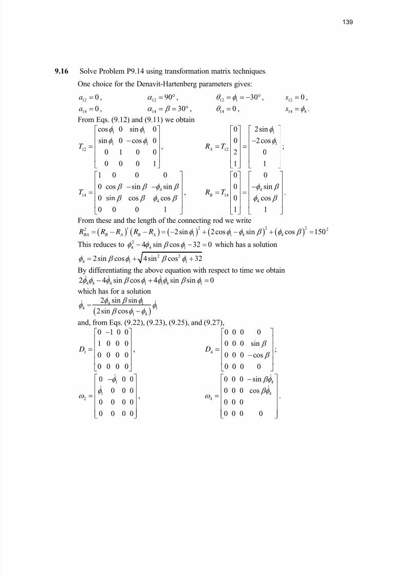
9.16 Solve Problem P9.14 using transformation matrix techniques.
One choice for the Denavit-Hartenberg parameters gives:
12 0a = , 12 90α = ° , 12 1 30θ φ = = − ° , 12 0s = ,
14 0a = , 14 30α β = = ° , 14 0θ = , 14 4s φ = .
From Eqs. (9.12) and (9.11) we obtain
1 1
1 1
12
cos 0 sin 0
sin 0 cos 0
0 1 0 0
0 0 0 1
T
φ φ
φ φ
⎡ ⎤⎢ ⎥−⎢ ⎥=⎢ ⎥⎢ ⎥⎣ ⎦
,
1
1
12
0 2sin
0 2cos
2 0
1 1
A R T
φ
φ
⎡ ⎤ ⎡ ⎤⎢ ⎥ ⎢ ⎥−⎢ ⎥ ⎢ ⎥= =⎢ ⎥ ⎢ ⎥⎢ ⎥ ⎢ ⎥⎣ ⎦ ⎣ ⎦
;
4
144
1 0 0 0
0 cos sin sin
0 sin cos cos
0 0 0 1
T
β β φ β
β β φ β
⎡ ⎤⎢ ⎥− −⎢ ⎥
= ⎢ ⎥⎢ ⎥⎣ ⎦
,
4
144
0 0
0 sin
0 cos
1 1
B R T
φ β
φ β
⎡ ⎤ ⎡ ⎤⎢ ⎥ ⎢ ⎥−⎢ ⎥ ⎢ ⎥
= =⎢ ⎥ ⎢ ⎥⎢ ⎥ ⎢ ⎥⎣ ⎦ ⎣ ⎦
.
From these and the length of the connecting rod we write
( ) ( ) ( ) ( ) ( )2 2 22 2
1 1 4 42sin 2cos sin cos 150t
BA B A B A R R R R R φ φ φ β φ β = − − = − + − + =
This reduces to 2
4 4 14 sin cos 32 0φ φ β φ − − = which has a solution
2 2
4 1 12sin cos 4sin cos 32φ β φ β φ = + +
By differentiating the above equation with respect to time we obtain
4 4 4 1 1 4 12 4 sin cos 4 sin sin 0φ φ φ β φ φ φ β φ − + =
which has for a solution
( )4 1
4 1
1 4
2 sin sin
2sin cos
φ β φ φ φ
β φ φ =
−
and, from Eqs. (9.22), (9.23), (9.25), and (9.27),
1
0 1 0 0
1 0 0 0
0 0 0 0
0 0 0 0
D
−⎡ ⎤⎢ ⎥⎢ ⎥=⎢ ⎥⎢ ⎥⎣ ⎦
, 4
0 0 0 0
0 0 0 sin
0 0 0 cos
0 0 0 0
D β
β
⎡ ⎤⎢ ⎥⎢ ⎥=⎢ ⎥−⎢ ⎥⎣ ⎦
;
1
12
0 0 0
0 0 0
0 0 0 0
0 0 0 0
φ
φ ω
⎡ ⎤−⎢ ⎥⎢ ⎥=⎢ ⎥⎢ ⎥⎢ ⎥⎣ ⎦
,
4
44
0 0 0 sin
0 0 0 cos
0 0 0
0 0 0 0
βφ
βφ ω
⎡ ⎤−⎢ ⎥⎢ ⎥=⎢ ⎥⎢ ⎥⎢ ⎥⎣ ⎦
.
8/10/2019 218 39 Solutions Instructor Manual Chapter 9 Spatial Mechanisms
http://slidepdf.com/reader/full/218-39-solutions-instructor-manual-chapter-9-spatial-mechanisms 14/21
140
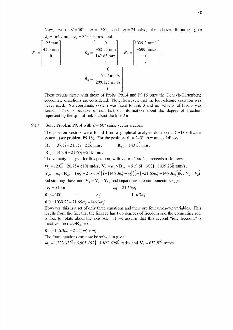
Now, with 30 β = ° , 1 30φ = − ° , and 1 24 rad/sφ = , the above formulae give
4 164.7 mmφ = , 4 345.4 mm/sφ = , and
25 mm
43.3 mm
01
A R
−⎡ ⎤⎢ ⎥⎢ ⎥=
⎢ ⎥⎢ ⎥⎣ ⎦
,
0
82.35 mm
142.65 mm1
B R
⎡ ⎤⎢ ⎥−⎢ ⎥=
⎢ ⎥⎢ ⎥⎣ ⎦
,
1039.2 mm/s
600 mm/s
00
A R
⎡ ⎤⎢ ⎥−⎢ ⎥=
⎢ ⎥⎢ ⎥⎣ ⎦
,
0
172.7 mm/s
299.125 mm/s
0
B R
⎡ ⎤⎢ ⎥−⎢ ⎥=⎢ ⎥⎢ ⎥⎣ ⎦
.
These results agree with those of Probs. P9.14 and P9.15 once the Denavit-Hartenbergcoordinate directions are considered. Note, however, that the loop-closure equation wasnever used. No coordinate system was fixed to link 3 and no velocity of link 3 was
found. This is because of our lack of information about the degree of freedomrepresenting the spin of link 3 about the line AB.
9.17 Solve Problem P9.14 with β = 60° using vector algebra.
The position vectors were found from a graphical analysis done on a CAD software
system; (see problem P9.18). For the position 2 240θ = ° they are as follows:
ˆ ˆ ˆ37.5 21.65 25 mm AO = + −R i j k , ˆ183.8 mm BO =R i ,
ˆ ˆ ˆ146.3 21.65 25 mm BA = − +R i j k .
The velocity analysis for this position, with 2 24 rad/sω = , proceeds as follows:
2
ˆ ˆ12.0 20.784 610 rad/s= −i j , 2
ˆ ˆ ˆ519.6 300 1039.23 mm/s A AOω = × = + +V R i j k ,
( ) ( ) ( )3 3 3 3 3 3 3ˆ ˆ ˆ21.65 146.3 21.65 146.3 y z z x x y
BA BAω ω ω ω ω ω ω = × = + + − + − −V R i j k , ˆ B BV =V i .
Substituting these into B A BA= +V V V and separating into components we get
3 3
3 3
3 3
519.6 21.65
0.0 300 146.3
0.0 1039.23 21.65 146.3
y z
B
x z
x y
V ω ω
ω ω
ω ω
= + +
= − +
= − −
However, this is a set of only three equations and there are four unknown variables. Thisresults from the fact that the linkage has two degrees of freedom and the connecting rodis free to rotate about the axis AB. If we assume that this second “idle freedom” is
inactive, then 3 0 BA =R i .
3 3 30.0 146.3 21.65 x y zω ω ω = − +
The four equations can now be solved to give
3ˆ ˆ ˆ1.333 333 6.905 692 1.822 629 rad/s= + −ω i j k and ˆ652.82 mm/s B =V i

8/10/2019 218 39 Solutions Instructor Manual Chapter 9 Spatial Mechanisms
http://slidepdf.com/reader/full/218-39-solutions-instructor-manual-chapter-9-spatial-mechanisms 15/21
141
9.18 Solve Problem P9.14 with β = 60° using graphical techniques.
9.19 Solve Problem P9.14 with β = 60° using transformation matrix techniques.One choice for the Denavit-Hartenberg parameters gives:
12 0a = , 12 90α = ° , 12 1 30θ φ = = − ° , 12 0s = ,
14 0a = , 14 60α β = = ° , 14 0θ = , 14 4s φ = .
From Eqs. (9.12) and (9.11) we obtain
1 1
1 1
12
cos 0 sin 0
sin 0 cos 0
0 1 0 0
0 0 0 1
T
φ φ
φ φ
⎡ ⎤⎢ ⎥−⎢ ⎥=⎢ ⎥⎢ ⎥⎣ ⎦
,
1
1
12
0 2sin
0 2cos
2 0
1 1
A R T
φ
φ
⎡ ⎤ ⎡ ⎤⎢ ⎥ ⎢ ⎥−⎢ ⎥ ⎢ ⎥= =⎢ ⎥ ⎢ ⎥⎢ ⎥ ⎢ ⎥⎣ ⎦ ⎣ ⎦
;
4
14
4
1 0 0 0
0 cos sin sin
0 sin cos cos
0 0 0 1
T β β φ β
β β φ β
⎡ ⎤⎢ ⎥− −⎢ ⎥=⎢ ⎥
⎢ ⎥⎣ ⎦
,4
14
4
0 0
0 sin
0 cos
1 1
B R T φ β
φ β
⎡ ⎤ ⎡ ⎤⎢ ⎥ ⎢ ⎥−⎢ ⎥ ⎢ ⎥= =⎢ ⎥ ⎢ ⎥
⎢ ⎥ ⎢ ⎥⎣ ⎦ ⎣ ⎦
.
From these and the length of the connecting rod we write
( ) ( ) ( ) ( ) ( )2 2 22 2
1 1 4 42sin 2cos sin cos 150t
BA B A B A R R R R R φ φ φ β φ β = − − = − + − + =
This reduces to 2
4 4 14 sin cos 32 0φ φ β φ − − = which has a solution
2 2
4 1 12sin cos 4sin cos 32φ β φ β φ = + +

8/10/2019 218 39 Solutions Instructor Manual Chapter 9 Spatial Mechanisms
http://slidepdf.com/reader/full/218-39-solutions-instructor-manual-chapter-9-spatial-mechanisms 16/21
142
By differentiating the above equation with respect to time we obtain
4 4 4 1 1 4 12 4 sin cos 4 sin sin 0φ φ φ β φ φ φ β φ − + =
which has for a solution
( )4 1
4 1
1 4
2 sin sin
2sin cos
φ β φ φ φ
β φ φ =
−
and, from Eqs. (9.22), (9.23), (9.25), and (9.27),
1
0 1 0 0
1 0 0 0
0 0 0 0
0 0 0 0
D
−⎡ ⎤⎢ ⎥⎢ ⎥=⎢ ⎥⎢ ⎥⎣ ⎦
, 4
0 0 0 0
0 0 0 sin
0 0 0 cos
0 0 0 0
D β
β
⎡ ⎤⎢ ⎥⎢ ⎥=⎢ ⎥−⎢ ⎥⎣ ⎦
;
1
12
0 0 0
0 0 0
0 0 0 0
0 0 0 0
φ
φ ω
⎡ ⎤−⎢ ⎥⎢ ⎥=⎢ ⎥⎢ ⎥
⎢ ⎥⎣ ⎦
,
4
44
0 0 0 sin
0 0 0 cos
0 0 0
0 0 0 0
βφ
βφ ω
⎡ ⎤−⎢ ⎥⎢ ⎥=⎢ ⎥⎢ ⎥
⎢ ⎥⎣ ⎦
.
Now, with 60 β = ° , 1 30φ = − ° , and 1 24 rad/sφ = , the above formulae give
4 183.8 mmφ = , 4 652.8 mm/sφ = , and
25 mm
43.3 mm
0
1
A R
−⎡ ⎤⎢ ⎥⎢ ⎥=⎢ ⎥⎢ ⎥⎣ ⎦
,
0
159.175 mm
91.9 mm
1
B R
⎡ ⎤⎢ ⎥−⎢ ⎥=⎢ ⎥⎢ ⎥⎣ ⎦
,
1039.225 mm/s
600 mm/s
0
0
A R
⎡ ⎤⎢ ⎥−
⎢ ⎥= ⎢ ⎥⎢ ⎥⎣ ⎦
,
0
565.35 mm/s
326.4 mm/s
0
B R
⎡ ⎤⎢ ⎥−⎢ ⎥=⎢ ⎥⎢ ⎥⎣ ⎦
.
These results agree with those of Probs. P9.17 and P9.18 once the Denavit-Hartenbergcoordinate directions are considered.
9.20
The figure shows the top, front, and profile views of an RGRC crank and oscillating-slider linkage. Link 4, the oscillating slider, is rigidly attached to a round rod that rotatesand slides in the two bearings. (a) Use the Kutzbach criterion to find the mobility of thislinkage. (b) With crank 2 as the driver, find the total angular and linear travel of link 4.(c) Write the loop-closure equation for this mechanism and use vector algebra to solve itfor all unknown position data.
a) The RGRC linkage has n = 4, j1 = 2, j2 = 1, j3 = 1. The Kutzbach criterion gives

8/10/2019 218 39 Solutions Instructor Manual Chapter 9 Spatial Mechanisms
http://slidepdf.com/reader/full/218-39-solutions-instructor-manual-chapter-9-spatial-mechanisms 17/21
143
( ) 1 2 36 1 5 4 3 6(4 1) 5(2) 4(1) 3(1) 1m n j j j= − − − − = − − − − = Ans.
b) Since vectors do not show the rotation θ 4, matrix methods were necessary and areshown in problem P9.23. See c) for the vector solution. Together, they show:
4135 45θ − ° < < − ° ; 4 90θ Δ = ° . Ans.
182.85 mm 382.85 mm B y< <
; 200 mm B yΔ =
. Ans. c) B AB Q AQ+ = +R R R R
2 2ˆ ˆ ˆ ˆ ˆˆ ˆ100 100sin 100cos B AB AB AB y x y z θ θ + + + = − − + j i j k i j k
Separating components,
100 AB x = − , 2100sin B AB y y θ + = − , 2100cos AB z θ =
and, from the length of link 3,2 2 2 2
AB AB AB AB x y z R+ + =
( ) ( ) ( )2 2 2 2
2 2100 100sin 100cos 300 B yθ θ − + − − + =
2
2200sin 2800 0 B B y yθ + − =
22 2100sin 100 175 sin B y θ θ = − + + Ans.
2
2 2ˆ ˆ ˆ100 100 175 sin 100cos AB θ θ = − − + +R i j k Ans.
For 2 40θ = ° , ˆ ˆ208 mm B B y= =R j j , ˆ ˆ ˆ100 272.275 76.6 mm AB = − − +R i j k . Ans.
9.21 Use vector algebra to find V B, 3, and 4 for Problem P9.20.
First we identify for 2 40θ = ° , that ˆ100 inQ = −R i , ˆ ˆ64.275 76.6 mm AQ = − +R j k ,
ˆ208 mm B =R j , and ˆ ˆ ˆ100 272.275 76.6 m AB = − − +R i j k .
Next we note that the rotation axis of the revolute at B is ˆ ˆ76.6 100 AB× = +R i k and,
normalizing this, we can express the apparent angular velocity 3/ 4ω axis by
3/ 4ˆ ˆˆ 0.608 0.794= +ω i k . Then the angular velocity of link 3 can be written as:
3 4 3/ 4 3/ 4 4 3/ 4ˆ ˆ ˆ0.608 0.794ω ω ω = + = + +ω ω ω i j k . With this done, we can find
2ˆ ˆ3677 3085.375 mm/s A AQ= = +V ω ×R j k , ˆ
B BV =V j , and
( )3 4 3/ 4 3/ 4 4 3/ 4ˆ ˆ ˆ(76.6 216.15 ) 125.975 100 165.575 AB AB ω ω ω ω ω = = + − + −V ω × R i j k . Now,
setting B AB A+ =V V V and separating components, we get the following equations
4 3/ 4
3/ 4
4 3/ 4
76.6 216.15 0
125.975 3677
100 165.575 3085.375
BV
ω ω
ω
ω ω
+ =
− =
− =
which can be solved to give 4 19.444 rad/sω = , 3/ 4 6.891 rad/sω = − , 2808.95 mm/s BV = .
3ˆ ˆ ˆ4.190 19.444 5.471 rad/s= − + −ω i j k , 4
ˆ19.444 rad/s=ω j , ˆ2808.95 mm/s B =V j . Ans.
Note that, if 3ω were written as 3 3 3 3ˆ ˆ ˆ x y zω ω ω = + +ω i j k , then the above set of simultaneous
equations would have would have four unknowns and could not be solved.

8/10/2019 218 39 Solutions Instructor Manual Chapter 9 Spatial Mechanisms
http://slidepdf.com/reader/full/218-39-solutions-instructor-manual-chapter-9-spatial-mechanisms 18/21
144
9.22 Solve Problem P9.21 using graphical techniques.
9.23 Solve Problem P9.21 using transformation matrix techniques.
The Denavit-Hartenberg parameters from the global coordinate system to joint A are:
12 0a = , 12 0α = , 12 2 40θ θ = = ° , 12 100 mms = − ,
and, proceeding in the other direction around the loop, to joint A, they are:
16 0a = , 16 90α = − ° , 16 0θ = , 16 0s = ,
65 0a = , 65 0α = , 65 0θ = , 65 Bs y= ,
54 0a = , 54 0α = , 54 4θ θ = , 54 0s = ,
43 0a = , 43 90α = ° , 43 0θ = , 43 0s = ,

8/10/2019 218 39 Solutions Instructor Manual Chapter 9 Spatial Mechanisms
http://slidepdf.com/reader/full/218-39-solutions-instructor-manual-chapter-9-spatial-mechanisms 19/21
145
3 0 B
a = , 3 0 B
α = , 3 3 Bθ θ = , 3 0
Bs = ,
300 mm BAa = , 0 BAα = , 90 BAθ = − , 0 BAs = .
From Eqs. (9.12) we obtain for the first path to A:
2 2
2 212
cos sin 0 0
sin cos 0 00 0 1 4
0 0 0 1
T
θ θ
θ θ
−⎡ ⎤⎢ ⎥
⎢ ⎥= ⎢ ⎥−⎢ ⎥⎣ ⎦
,
and along the other path to joint A, from Eqs. (9.12) and (9.15), we get:
16
1 0 0 0
0 0 1 0
0 1 0 0
0 0 0 1
T
⎡ ⎤⎢ ⎥⎢ ⎥=⎢ ⎥−⎢ ⎥⎣ ⎦
,
65
1 0 0 0
0 1 0 0
0 0 1
0 0 0 1
B
T y
⎡ ⎤
⎢ ⎥⎢ ⎥=⎢ ⎥⎢ ⎥⎣ ⎦
, 15
1 0 0 0
0 0 1
0 1 0 0
0 0 0 1
B yT
⎡ ⎤
⎢ ⎥⎢ ⎥=⎢ ⎥−⎢ ⎥⎣ ⎦
,
4 4
4 4
54
cos sin 0 0
sin cos 0 0
0 0 1 0
0 0 0 1
T
θ θ
θ θ
−⎡ ⎤⎢ ⎥⎢ ⎥=⎢ ⎥⎢ ⎥⎣ ⎦
,
4 4
14
4 4
cos sin 0 0
0 0 1
sin cos 0 0
0 0 0 1
B y
T
θ θ
θ θ
−⎡ ⎤⎢ ⎥⎢ ⎥=⎢ ⎥− −⎢ ⎥⎣ ⎦
,
43
1 0 0 0
0 0 1 0
0 1 0 0
0 0 0 1
T
⎡ ⎤⎢ ⎥−⎢ ⎥=⎢ ⎥⎢ ⎥⎣ ⎦
,
4 4
13
4 4
cos 0 sin 0
0 1 0
sin 0 cos 0
0 0 0 1
B y
T
θ θ
θ θ
⎡ ⎤⎢ ⎥⎢ ⎥=⎢ ⎥−⎢ ⎥⎣ ⎦
,
3 3
3 3
3
cos sin 0 0
sin cos 0 0
0 0 1 0
0 0 0 1
BT
θ θ
θ θ
−⎡ ⎤⎢ ⎥⎢ ⎥=⎢ ⎥⎢ ⎥⎣ ⎦
,
3 4 3 4 4
3 3
1
3 4 3 4 4
cos cos sin cos sin 0
sin cos 0
cos sin sin sin cos 0
0 0 0 1
B
B
yT
θ θ θ θ θ
θ θ
θ θ θ θ θ
−⎡ ⎤⎢ ⎥⎢ ⎥=⎢ ⎥−⎢ ⎥⎣ ⎦
,
0 1 0 01 0 0 12
0 0 1 0
0 0 0 1
BAT
⎡ ⎤⎢ ⎥− −⎢ ⎥=⎢ ⎥⎢ ⎥⎣ ⎦
,
3 4 3 4 4 3 4
3 3 3
1
3 4 3 4 4 3 4
sin cos cos cos sin 12sin coscos sin 0 12cos
sin sin cos sin cos 12sin sin
0 0 0 1
B
A
yT
θ θ θ θ θ θ θ θ θ θ
θ θ θ θ θ θ θ
⎡ ⎤⎢ ⎥− −⎢ ⎥=⎢ ⎥− − −⎢ ⎥⎣ ⎦
.
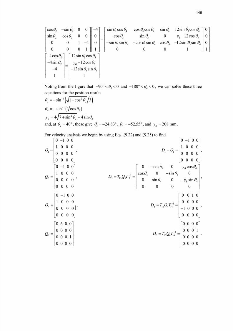
At the terminations of these two paths, the position of point A must agree. Therefore
8/10/2019 218 39 Solutions Instructor Manual Chapter 9 Spatial Mechanisms
http://slidepdf.com/reader/full/218-39-solutions-instructor-manual-chapter-9-spatial-mechanisms 20/21
146
2 2 3 4 3 4 4 3 4
2 2 3 3 3
3 4 3 4 4 3 4
cos sin 0 0 4 sin cos cos cos sin 12sin cos 0
sin cos 0 0 0 cos sin 0 12cos 0
0 0 1 4 0 sin sin cos sin cos 12sin sin 0
0 0 0 1 1 0 0 0 1 1
B y
θ θ θ θ θ θ θ θ θ
θ θ θ θ θ
θ θ θ θ θ θ θ
− −⎡ ⎤ ⎡ ⎤ ⎡ ⎤ ⎡ ⎤⎢ ⎥ ⎢ ⎥ ⎢ ⎥ ⎢ ⎥− −⎢ ⎥ ⎢ ⎥ ⎢ ⎥ ⎢ ⎥=⎢ ⎥ ⎢ ⎥ ⎢ ⎥ ⎢ ⎥− − − −⎢ ⎥ ⎢ ⎥ ⎢ ⎥ ⎢ ⎥⎣ ⎦ ⎣ ⎦ ⎣ ⎦ ⎣ ⎦
2 3 4
2 3
3 4
4cos 12sin cos4sin 12cos
4 12sin sin
1 1
B y
θ θ θ θ θ
θ θ
−⎡ ⎤ ⎡ ⎤⎢ ⎥ ⎢ ⎥− −⎢ ⎥ ⎢ ⎥=⎢ ⎥ ⎢ ⎥− −⎢ ⎥ ⎢ ⎥⎣ ⎦ ⎣ ⎦
Noting from the figure that 390 0θ − ° < < and 4180 0θ − ° < < , we can solve these three
equations for the position results
( )1 2
3 2sin 1 cos 3θ θ −= − +
( )1
4 2tan 1 cosθ θ −= −
2
2 24 7 sin 4sin B y θ θ = + −
and, at 2 40θ = ° , these give 3 24.83θ = − ° , 4 52.55θ = − ° , and 208 mm B y = .
For velocity analysis we begin by using Eqs. (9.22) and (9.25) to find
1
0 1 0 0
1 0 0 0
0 0 0 0
0 0 0 0
Q
−⎡ ⎤⎢ ⎥⎢ ⎥=⎢ ⎥⎢ ⎥⎣ ⎦
, 1 1
0 1 0 0
1 0 0 0
0 0 0 0
0 0 0 0
D Q
−⎡ ⎤⎢ ⎥⎢ ⎥= =⎢ ⎥⎢ ⎥⎣ ⎦
,
3
0 1 0 01 0 0 0
0 0 0 0
0 0 0 0
Q
−⎡ ⎤⎢ ⎥⎢ ⎥=⎢ ⎥⎢ ⎥⎣ ⎦
,
4 4
4 41
3 13 3 13
4 4
0 cos 0 coscos 0 sin 0
0 sin 0 sin
0 0 0 0
B
B
y
D T Q T y
θ θ θ θ
θ θ
−
−⎡ ⎤⎢ ⎥−⎢ ⎥= =⎢ ⎥−⎢ ⎥⎣ ⎦
,
4
0 1 0 0
1 0 0 0
0 0 0 0
0 0 0 0
Q
−⎡ ⎤⎢ ⎥⎢ ⎥=⎢ ⎥⎢ ⎥⎣ ⎦
, 1
4 14 4 14
0 0 1 0
0 0 0 0
1 0 0 0
0 0 0 0
D T Q T −
⎡ ⎤⎢ ⎥⎢ ⎥= =⎢ ⎥−⎢ ⎥⎣ ⎦
,
6
0 6 0 00 0 0 0
0 0 0 1
0 0 0 0
Q
⎡ ⎤⎢ ⎥⎢ ⎥=⎢ ⎥⎢ ⎥⎣ ⎦
, 1
6 16 6 16
0 0 0 00 0 0 1
0 0 0 0
0 0 0 0
D T Q T −
⎡ ⎤⎢ ⎥⎢ ⎥= =⎢ ⎥⎢ ⎥⎣ ⎦
.

8/10/2019 218 39 Solutions Instructor Manual Chapter 9 Spatial Mechanisms
http://slidepdf.com/reader/full/218-39-solutions-instructor-manual-chapter-9-spatial-mechanisms 21/21
147
Next we write from Eq. (9.27)
2
22 2 2
0 0 0
0 0 0
0 0 0 0
0 0 0 0
D
θ
θ ω θ
⎡ ⎤−⎢ ⎥⎢ ⎥= =⎢ ⎥⎢ ⎥
⎢ ⎥⎣ ⎦
and, along the other path,
4 3 4 4 3
4 3 4 33 6 4 4 3 3
4 4 3 4 3
0 cos cos
cos 0 sin
sin 0 sin
0 0 0 0
B
B
B
B
y
y D y D D
y
θ θ θ θ θ
θ θ θ θ ω θ θ
θ θ θ θ θ
⎡ ⎤−⎢ ⎥
−⎢ ⎥= + + =⎢ ⎥− −⎢ ⎥⎢ ⎥⎣ ⎦
4
4 6 4 4
4
0 0 0
0 0 0
0 0 0
0 0 0 0
B
B
y D y D
θ
ω θ θ
⎡ ⎤⎢ ⎥⎢ ⎥= + =⎢ ⎥−
⎢ ⎥⎢ ⎥⎣ ⎦
Since the velocity of point A must agree along the two paths
2 2
2 2
2 3
4cos 4cos
4sin 4sin
4 4
1 1
θ θ
θ θ ω ω
− −⎡ ⎤ ⎡ ⎤⎢ ⎥ ⎢ ⎥− −⎢ ⎥ ⎢ ⎥=⎢ ⎥ ⎢ ⎥− −⎢ ⎥ ⎢ ⎥⎣ ⎦ ⎣ ⎦
2 2 2 4 3 4 3 4
2 2 2 4 3 4 3
2 4 2 4 3 4 3
4sin 4sin cos cos 4
4cos 4cos cos 4sin
0 4cos 4sin sin sin
0 0
B
B
B
y
y
y
θ θ θ θ θ θ θ θ
θ θ θ θ θ θ θ
θ θ θ θ θ θ θ
⎡ ⎤ ⎡ ⎤− + −⎢ ⎥ ⎢ ⎥
− − + +⎢ ⎥ ⎢ ⎥=
⎢ ⎥ ⎢ ⎥− −⎢ ⎥ ⎢ ⎥⎢ ⎥ ⎢ ⎥⎣ ⎦ ⎣ ⎦
At the position where 2 40θ = ° , 3 24.83θ = − ° , 4 52.55θ = − ° , 208 mm B y = , and
2 48.0 rad/sθ = − , these equations can be solved for 3 6.891 rad/sθ = , 4 19.444 rad/sθ = ,
and 2808.95 mm/s B y = . With these values we can evaluate
3
0 4.191 19.444 34.865
4.191 0 5.471 112.357
19.444 5.471 0 45.513
0 0 0 0
ω
−⎡ ⎤⎢ ⎥⎢ ⎥=⎢ ⎥− −⎢ ⎥
⎣ ⎦
and 4
0 0 19.444 0
0 0 0 112.357
19.444 0 0 0
0 0 0 0
ω
⎡ ⎤⎢ ⎥⎢ ⎥=⎢ ⎥−⎢ ⎥
⎣ ⎦
from
which we write the vector forms of the results:ˆ2808.95 mm/s B =V j , 3
ˆ ˆ ˆ5.471 19.444 4.191 rad/s= − + +ω i j k , and 4ˆ19.444 rad/s=ω j . Ans.
Note that the global x1 and z1 axis orientations in this solution differ from those of problem P9.21 because of the conventions of the Denavit-Hartenberg parameters. This is
the reason that the components of ω 3 seem switched.