216 CHAPTER 3 Linear Algebra 3.2 216 CHAPTER 3 …APPM 2360 Homework 5 Solutions Fall 2015 Section...

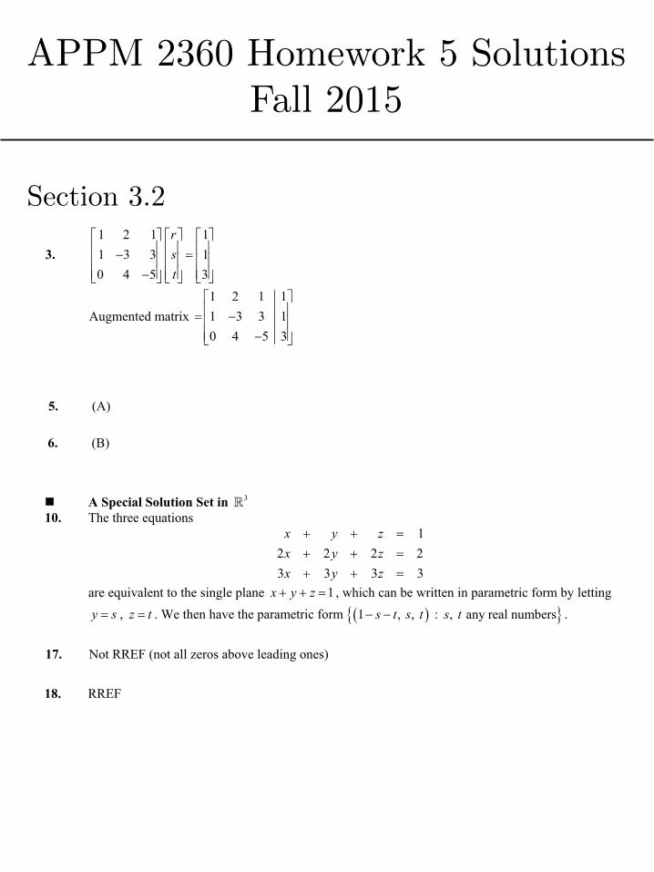
APPM 2360 Homework 5 SolutionsFall 2015

Section 3.2

216 CHAPTER 3 Linear Algebra

3.2 Systems of Linear Equations

� Matrix-Vector Form

1. 1 2 12 1 03 2 1

xy

ª º ª ºª º« » « »� « »« » « »¬ ¼« » « »¬ ¼ ¬ ¼

2.

1

2

3

4

1 2 1 3 21 3 3 0 1

iiii

ª º« »ª º ª º« » « » « »« »�¬ ¼ ¬ ¼« »¬ ¼

Augmented matrix 1 2 12 1 03 2 1

ª º« » �« »« »¬ ¼

Augmented matrix 1 2 1 3 21 3 3 0 1ª º

« »�¬ ¼

3. 1 2 1 11 3 3 10 4 5 3

rst

ª º ª º ª º« » « » « »� « » « » « »« » « » « »�¬ ¼ ¬ ¼ ¬ ¼

4. > @1

2

3

1 2 3 0xxx

ª º« »� « »« »¬ ¼

Augmented matrix 1 2 1 11 3 3 10 4 5 3

ª º« » �« »« »�¬ ¼

Augmented matrix > @1 2 3 | 0 �

� Solutions in 2� 5. (A) 6. (B) 7. (C) 8. (B) 9. (A) � A Special Solution Set in 3� 10. The three equations

1

2 2 2 23 3 3 3

x y zx y zx y z

� � � � � �

are equivalent to the single plane 1x y z� � , which can be written in parametric form by letting

y s , z t . We then have the parametric form � �^ `1 , , : , any real numberss t s t s t� � . � Reduced Row Echelon Form 11. RREF 12. Not RREF (not all zeros above leading ones) 13. Not RREF (leading nonzero element in row 2 is not 1; not all zeros above the leading ones) 14. Not RREF (row 3 does not have a leading one, nor does it move to the right; plus pivot columns

have nonzero entries other than the leading ones) 15. RREF 16. Not RREF (not all zeros above leading ones) 17. Not RREF (not all zeros above leading ones) 18. RREF 19. RREF




1. 1 2 12 1 03 2 1

xy

ª º ª ºª º« » « »� « »« » « »¬ ¼« » « »¬ ¼ ¬ ¼

2.

1

2

3

4

1 2 1 3 21 3 3 0 1

iiii

ª º« »ª º ª º« » « » « »« »�¬ ¼ ¬ ¼« »¬ ¼


ª º« » �« »« »¬ ¼


« »�¬ ¼

3. 1 2 1 11 3 3 10 4 5 3

rst

ª º ª º ª º« » « » « »� « » « » « »« » « » « »�¬ ¼ ¬ ¼ ¬ ¼

4. > @1

2

3

1 2 3 0xxx

ª º« »� « »« »¬ ¼


ª º« » �« »« »�¬ ¼



1

2 2 2 23 3 3 3

x y zx y zx y z

� � � � � �







1. 1 2 12 1 03 2 1

xy

ª º ª ºª º« » « »� « »« » « »¬ ¼« » « »¬ ¼ ¬ ¼

2.

1

2

3

4

1 2 1 3 21 3 3 0 1

iiii

ª º« »ª º ª º« » « » « »« »�¬ ¼ ¬ ¼« »¬ ¼


ª º« » �« »« »¬ ¼


« »�¬ ¼

3. 1 2 1 11 3 3 10 4 5 3

rst

ª º ª º ª º« » « » « »� « » « » « »« » « » « »�¬ ¼ ¬ ¼ ¬ ¼

4. > @1

2

3

1 2 3 0xxx

ª º« »� « »« »¬ ¼


ª º« » �« »« »�¬ ¼



1

2 2 2 23 3 3 3

x y zx y zx y z

� � � � � �







1. 1 2 12 1 03 2 1

xy

ª º ª ºª º« » « »� « »« » « »¬ ¼« » « »¬ ¼ ¬ ¼

2.

1

2

3

4

1 2 1 3 21 3 3 0 1

iiii

ª º« »ª º ª º« » « » « »« »�¬ ¼ ¬ ¼« »¬ ¼


ª º« » �« »« »¬ ¼


« »�¬ ¼

3. 1 2 1 11 3 3 10 4 5 3

rst

ª º ª º ª º« » « » « »� « » « » « »« » « » « »�¬ ¼ ¬ ¼ ¬ ¼

4. > @1

2

3

1 2 3 0xxx

ª º« »� « »« »¬ ¼


ª º« » �« »« »�¬ ¼



1

2 2 2 23 3 3 3

x y zx y zx y z

� � � � � �







1. 1 2 12 1 03 2 1

xy

ª º ª ºª º« » « »� « »« » « »¬ ¼« » « »¬ ¼ ¬ ¼

2.

1

2

3

4

1 2 1 3 21 3 3 0 1

iiii

ª º« »ª º ª º« » « » « »« »�¬ ¼ ¬ ¼« »¬ ¼


ª º« » �« »« »¬ ¼


« »�¬ ¼

3. 1 2 1 11 3 3 10 4 5 3

rst

ª º ª º ª º« » « » « »� « » « » « »« » « » « »�¬ ¼ ¬ ¼ ¬ ¼

4. > @1

2

3

1 2 3 0xxx

ª º« »� « »« »¬ ¼


ª º« » �« »« »�¬ ¼



1

2 2 2 23 3 3 3

x y zx y zx y z

� � � � � �







1. 1 2 12 1 03 2 1

xy

ª º ª ºª º« » « »� « »« » « »¬ ¼« » « »¬ ¼ ¬ ¼

2.

1

2

3

4

1 2 1 3 21 3 3 0 1

iiii

ª º« »ª º ª º« » « » « »« »�¬ ¼ ¬ ¼« »¬ ¼


ª º« » �« »« »¬ ¼


« »�¬ ¼

3. 1 2 1 11 3 3 10 4 5 3

rst

ª º ª º ª º« » « » « »� « » « » « »« » « » « »�¬ ¼ ¬ ¼ ¬ ¼

4. > @1

2

3

1 2 3 0xxx

ª º« »� « »« »¬ ¼


ª º« » �« »« »�¬ ¼



1

2 2 2 23 3 3 3

x y zx y zx y z

� � � � � �




SECTION 3.2 Systems of Linear Equations 217

� Gauss-Jordan Elimination

20. Starting with 1 3 8 00 1 2 10 1 2 4

ª º« »« »« »¬ ¼

� �3 3 21R R R � � 1 3 8 00 1 2 10 0 0 3

ª º« »« »« »¬ ¼

3 313

R R 1 3 8 00 1 2 10 0 0 1

ª º« »« »« »¬ ¼

.

This matrix is in row echelon form. To further reduce it to RREF we carry out the following

elementary row operations � �1 1 23R R R � � , � �2 2 31R R R � �

1 0 2 00 1 2 0 RREF0 0 0 1

ª º« » m« »« »¬ ¼

.

Hence, we see the leading ones in this RREF form are in columns 1, 2, and 4, so the pivot columns of the original matrix are columns 1, 2, and 4 shown in bold and underlined as follows:

822

ª º« »« »« »¬ ¼

1 3 00 1 10 1 4

.

21. 0 0 2 2 22 2 6 14 4

�ª º« »¬ ¼

1 2R Rl 2 2 6 14 40 0 2 2 2ª º« »�¬ ¼

1 112

R R 1 1 3 7 20 0 2 2 2ª º« »�¬ ¼

2 212

R R 1 1 3 7 20 0 1 1 1ª º« »�¬ ¼

.

The matrix is in row echelon form. To further reduce it to RREF we carry out the following

elementary row operation.

� �1 1 23R R R � � 1 1 0 4 5

RREF0 0 1 1 1ª º

m« »�¬ ¼

The pivot columns of the original matrix are first and third.

0 2 22 14 4

�ª º« »¬ ¼

0 22 6

.


29. 1 4 5 02 1 8 9

�ª º« »�¬ ¼

� �2 2 12R R R � � 1 4 5 00 9 18 9

�ª º« »�¬ ¼

2 219

R R � 1 4 5 00 1 2 1

�ª º« »� �¬ ¼

� �1 1 24R R R � � RREF 1 0 3 40 1 2 1ª º« »� �¬ ¼

nonunique solutions; 1 34 3x x � , 2 31 2x x � � , 3x is arbitrary

30. 1 0 1 22 3 5 43 2 1 4

ª º« »�« »« »�¬ ¼

� �

� �

2 2 1

3 3 1

2

3

R R R

R R R

� �

� �

1 0 1 20 3 3 00 2 4 2

ª º« »�« »« »� �¬ ¼

2 213

R R � 1 0 1 20 1 1 00 2 4 2

ª º« »�« »« »� �¬ ¼

� �3 3 22R R R � � 1 0 1 20 1 1 00 0 2 2

ª º« »�« »« »� �¬ ¼

3 312

R R � 1 0 1 20 1 1 00 0 1 1

ª º« »�« »« »¬ ¼

� �1 1 3

2 2 3

1R R R

R R R

� �

�

RREF 1 0 0 10 1 0 10 0 1 1

ª º« »« »« »¬ ¼

unique solution; 1x y z

31. 1 1 1 01 1 0 01 2 1 0

�ª º« »« »« »�¬ ¼

� �

� �

2 2 1

3 3 1

1

1

R R R

R R R

� �

� �

1 1 1 00 2 1 00 3 2 0

�ª º« »�« »« »�¬ ¼

2 212

R R

1 1 1 010 1 02

0 3 2 0

�ª º« »« »�« »« »�¬ ¼

� �

1 1 2

3 3 23

R R R

R R R

�

� �

11 0 0210 1 0210 0 02

ª º« »« »« »�« »« »« »�« »¬ ¼

� �3 32R R �

11 0 0210 1 02

0 0 1 0

ª º« »« »« »�« »« »« »« »¬ ¼

1 1 3

2 2 3

12

12

R R R

R R R

§ · � �¨ ¸© ¹

�

RREF 1 0 0 00 1 0 00 0 1 0

ª º« »« »« »¬ ¼



29. 1 4 5 02 1 8 9

�ª º« »�¬ ¼

� �2 2 12R R R � � 1 4 5 00 9 18 9

�ª º« »�¬ ¼

2 219

R R � 1 4 5 00 1 2 1

�ª º« »� �¬ ¼

� �1 1 24R R R � � RREF 1 0 3 40 1 2 1ª º« »� �¬ ¼

nonunique solutions; 1 34 3x x � , 2 31 2x x � � , 3x is arbitrary

30. 1 0 1 22 3 5 43 2 1 4

ª º« »�« »« »�¬ ¼

� �

� �

2 2 1

3 3 1

2

3

R R R

R R R

� �

� �

1 0 1 20 3 3 00 2 4 2

ª º« »�« »« »� �¬ ¼

2 213

R R � 1 0 1 20 1 1 00 2 4 2

ª º« »�« »« »� �¬ ¼

� �3 3 22R R R � � 1 0 1 20 1 1 00 0 2 2

ª º« »�« »« »� �¬ ¼

3 312

R R � 1 0 1 20 1 1 00 0 1 1

ª º« »�« »« »¬ ¼

� �1 1 3

2 2 3

1R R R

R R R

� �

�

RREF 1 0 0 10 1 0 10 0 1 1

ª º« »« »« »¬ ¼


31. 1 1 1 01 1 0 01 2 1 0

�ª º« »« »« »�¬ ¼

� �

� �

2 2 1

3 3 1

1

1

R R R

R R R

� �

� �

1 1 1 00 2 1 00 3 2 0

�ª º« »�« »« »�¬ ¼

2 212

R R

1 1 1 010 1 02

0 3 2 0

�ª º« »« »�« »« »�¬ ¼

� �

1 1 2

3 3 23

R R R

R R R

�

� �

11 0 0210 1 0210 0 02

ª º« »« »« »�« »« »« »�« »¬ ¼

� �3 32R R �

11 0 0210 1 02

0 0 1 0

ª º« »« »« »�« »« »« »« »¬ ¼

1 1 3

2 2 3

12

12

R R R

R R R

§ · � �¨ ¸© ¹

�

RREF 1 0 0 00 1 0 00 0 1 0

ª º« »« »« »¬ ¼



38. In Problem 25, 36ª º« »¬ ¼

is a unique solution so $ = ^ `0G and

xG = 36ª º« »¬ ¼

+ 0G

39. In Problem 26, infinitely many solutions, 1

1 zz

ª º« »�« »« »¬ ¼

, and $ = 01 :

1r

½ª º° °« »� �® ¾« »° °« »¬ ¼¯ ¿

\

hence xG = 1 01 10 1

r�ª º ª º« » « »� �« » « »« » « »¬ ¼ ¬ ¼

for any r �\

40. In Problem 27, (already a homogeneous system), infinitely many solutions,

$ = 3

5 :7

r r ½�ª º° °« » �® ¾« »° °« »¬ ¼¯ ¿

\ and xG = 000

ª º« »« »« »¬ ¼

+ 357

r�ª º« »« »« »¬ ¼

for any r �\

41. In Problem 28,

231313

ª º« »« »« »« »« »« »�« »¬ ¼

is a unique solution so that $ = ^ `0G and xG

231313

ª º« »« »« »« »« »« »�« »¬ ¼

+ 0G

42. In Problem 29, infinitely many solutions: x1 = 4 � 3x3 x2 = �1 + 2x3, x3 arbitrary

$ = 32 :1

r r ½�ª º° °« » �® ¾« »° °« »¬ ¼¯ ¿

\

410

ª º« » �« »« »¬ ¼

xG + 321

r�ª º« »« »« »¬ ¼

for any r �\

43. In Problem 30, unique solution 111

ª º« »« »« »¬ ¼

so $ = ^ `0G and

111

ª º« » �« »« »¬ ¼

x 0GG


44. In Problem 31, unique solution 000

ª º« »« »« »¬ ¼

so $�= ^ `0G and

� x 0 0 0G G GG .

45. In Problem 32, infinitely many solutions x = �z, y = �z, z arbitrary, so

$ = 11 :1

r r ½�ª º° °« »� �® ¾« »° °« »¬ ¼¯ ¿

\

1

= 11

r�ª º« »� �« »« »¬ ¼

x 0GG for any r �\

46. In Problem 33, nonunique solutions: x = 1 � z, y = �z, z arbitrary,

$ = 11 :1

r r ½�ª º° °« »� �® ¾« »° °« »¬ ¼¯ ¿

\

1 10 10 1

r�ª º ª º

« » « » � �« » « »« » « »¬ ¼ ¬ ¼

xG for any r �\

47. In Problem 34, $ =

00

:01

r r

½ª º° °« »° °« » �® ¾« »° °« »° °¬ ¼¯ ¿

\ . However, the system is inconsistent so that there is no xp

and no general solution.

48. In Problem 35, there is a unique solution: x = 245

, y = 45

, z = 225

� so

$ = ^ `0G

and

24545

225

ª º« »« »« » �« »« »« »�« »¬ ¼

x 0GG .


49. In Problem 36, there are infinitely many solutions: x1 = 1 � 2x3 + 4x4, x2 = 2 � x3 + 3x4,

x3 is arbitrary, x4 is arbitrary.

$ =

2 41 3

: ,1 00 1

r s r s

½�ª º ª º° °« » « »�° °« » « »� �® ¾« » « »° °« » « »° °¬ ¼ ¬ ¼¯ ¿

\ ,

1 2 42 1 30 1 00 0 1

r s

�ª º ª º ª º« » « » « »�« » « » « » � �« » « » « »« » « » « »¬ ¼ ¬ ¼ ¬ ¼

xG for ,r s�\

� The RREF Example 50. Starting with the augmented matrix, we carry out the following steps

1 0 2 0 1 4 80 2 0 2 4 6 60 0 1 0 0 2 23 0 0 1 5 3 120 2 0 0 0 0 6

ª º« »� � �« »« »« »« »« »� �¬ ¼

� �

2 2

4 4 1

12

3

R R

R R R

� �

1 0 2 0 1 4 80 1 0 1 2 3 30 0 1 0 0 2 20 0 6 1 2 9 120 2 0 0 0 0 6

ª º« »� � �« »« »« »� � �« »« »� �¬ ¼

(We leave the next steps for the reader)

RREF =

1 0 0 0 1 0 40 1 0 0 0 0 30 0 1 0 0 2 20 0 0 1 2 3 00 0 0 0 0 0 0

ª º« »« »« »« »« »« »¬ ¼

� More Equations Than Variables 51. Converting the augmented matrix to RREF yields

3 5 0 1 1 0 0 23 7 3 8 0 1 0 10 5 0 5 0 0 1 30 2 3 7 0 0 0 01 4 1 1 0 0 0 0

ª º ª º« » « »�« » « »« » « »o�« » « »« » « »« » « »¬ ¼ ¬ ¼

consistent system; unique solution 2, 1x y � , 3z . � Consistency 52. A homogeneous system Ax 0

GG always has at least one solution, namely the zero vector x 0GG .


� Homogeneous Systems 53. The equations are

2 5 0

2 0w x z

y z� �

�

If we let and x r z s , we can solve 2y s � , 2 5w r s � . The solution is a plane in 4� given by

2 5 2 51 0

2 0 20 1

w r sx r

r sy sz s

� �ª º ª º ª º ª º« » « » « » « »« » « » « » « » �« » « » « » « »� �« » « » « » « »¬ ¼ ¬ ¼ ¬ ¼ ¬ ¼

,

for r, s any real numbers. 54. The equations are

2 0

0x z

y�

If we let ,z s we have 2x s � and hence the solution is a line in 3� given by

2 20 0

1

x sy sz s

� �ª º ª º ª º« » « » « » « » « » « »« » « » « »¬ ¼ ¬ ¼ ¬ ¼

.

55. The equation is

1 2 3 44 3 0 0x x x x� � � . If we let 2x r , 3x s , 4x t , we can solve

1 2 34 3 4 3x x x r s � � . Hence

1

2

3

4

4 3 4 3 01 0 00 1 00 0 1

x r sx r

r s tx sx t

� �ª º ª º ª º ª º ª º« » « » « » « » « »« » « » « » « » « » � �« » « » « » « » « »« » « » « » « » « »

¬ ¼ ¬ ¼ ¬ ¼ ¬ ¼¬ ¼

where r, s, t are any real numbers. � Making Systems Inconsistent

56. 1 0 30 2 41 0 5

ª º« »« »« »¬ ¼

*2 2

*3 1 3

1 2

R R

R R R

� �

1 0 30 1 20 0 2

ª º« »« »« »¬ ¼

*3 3

12

R R 1 0 30 1 20 0 1

ª º« »« »« »¬ ¼

Rank = 3 because every column is a pivot column.


*3 2 3R R R � �

1 1 20 3 3 20 0 0 2

aa b

a b c

ª º« »� � � �« »« »� � �¬ ¼

Any vector abc

ª º« »« »« »¬ ¼

for which �2a � b + c z 0

60. 1 1 11 1 01 2 1

�ª º« »« »« »�¬ ¼

*2 1 2

*3 1 3

R R RR R R

� �

� � 1 1 10 2 10 3 2

�ª º« »�« »« »�¬ ¼

*2 2

12

R R

1 1 110 12

0 3 2

�ª º« »« »�« »« »�¬ ¼

*1 2 1

*3 2 33

R R RR R R

�

� �

11 0210 1220 03

ª º« »« »« »�« »« »« »« »¬ ¼

*3 2

32

R R

11 0210 18

0 0 1

ª º« »« »« »�« »« »« »« »¬ ¼

*1 3 1

*2 3 2

1218

R R R

R R R

� �

� �

1 0 00 1 00 0 1

ª º« »« »« »¬ ¼

? rank A = 3

� Seeking Consistency 61. 4k z 62. Any k will produce a consistent system 63. 1k z r 64. The system is inconsistent for all k because the last two equations are parallel and distinct.

65. 1 0 0 1 20 2 4 0 61 1 2 1 12 2 4 2 k

ª º« »« »« »� � �« »¬ ¼

*2 2

*3 1 3

*4 1 4

12

2

R R

R R RR R R

� �

� �

1 0 0 1 20 1 2 0 30 1 2 0 30 2 4 0 4 k

ª º« »« »« »� � �« »� �¬ ¼

*3 2 3

*4 1 42

R R RR R R

�

� �

1 0 0 1 20 1 2 0 30 0 0 0 00 0 0 0 10 k

ª º« »« »« »« »� �¬ ¼

Consistent if k = 10.


*3 2 3R R R � �

1 1 20 3 3 20 0 0 2

aa b

a b c

ª º« »� � � �« »« »� � �¬ ¼

Any vector abc

ª º« »« »« »¬ ¼

for which �2a � b + c z 0

60. 1 1 11 1 01 2 1

�ª º« »« »« »�¬ ¼

*2 1 2

*3 1 3

R R RR R R

� �

� � 1 1 10 2 10 3 2

�ª º« »�« »« »�¬ ¼

*2 2

12

R R

1 1 110 12

0 3 2

�ª º« »« »�« »« »�¬ ¼

*1 2 1

*3 2 33

R R RR R R

�

� �

11 0210 1220 03

ª º« »« »« »�« »« »« »« »¬ ¼

*3 2

32

R R

11 0210 18

0 0 1

ª º« »« »« »�« »« »« »« »¬ ¼

*1 3 1

*2 3 2

1218

R R R

R R R

� �

� �

1 0 00 1 00 0 1

ª º« »« »« »¬ ¼

? rank A = 3

� Seeking Consistency 61. 4k z 62. Any k will produce a consistent system 63. 1k z r 64. The system is inconsistent for all k because the last two equations are parallel and distinct.

65. 1 0 0 1 20 2 4 0 61 1 2 1 12 2 4 2 k

ª º« »« »« »� � �« »¬ ¼

*2 2

*3 1 3

*4 1 4

12

2

R R

R R RR R R

� �

� �

1 0 0 1 20 1 2 0 30 1 2 0 30 2 4 0 4 k

ª º« »« »« »� � �« »� �¬ ¼

*3 2 3

*4 1 42

R R RR R R

�

� �

1 0 0 1 20 1 2 0 30 0 0 0 00 0 0 0 10 k

ª º« »« »« »« »� �¬ ¼

Consistent if k = 10.


� Tandem with a Twist 72. (a) We place the right-hand sides of the two systems in the last two columns of the

augmented matrix

1 1 0 3 50 2 1 2 4ª º« »¬ ¼

.

Reducing this matrix to RREF, yields

11 0 2 3210 1 1 22

ª º�« »« »« »« »¬ ¼

.

Hence, the first system has solutions 122

x z � , 112

y z � , z arbitrary, and the second

system has solutions 132

x z � , 122

y z � , z arbitrary.

(b) If you look carefully, you will see that the matrix equation

11 12

21 22

31 32

1 1 0 3 50 2 1 2 4

x xx xx x

ª ºª º ª º« » « » « »« »¬ ¼ ¬ ¼« »¬ ¼

is equivalent to the two systems of equations

11

21

31

12

22

32

1 1 0 30 2 1 2

1 1 0 5.

0 2 1 4

xxx

xxx

ª ºª º ª º« » « » « »« »¬ ¼ ¬ ¼« »¬ ¼

ª ºª º ª º« » « » « »« »¬ ¼ ¬ ¼« »¬ ¼

We saw in part (a) that the solution of the system on the left was

11 31122

x x � , 21 31112

x x � , 31x arbitrary,

and the solution of the system on the right was

12 32132

x x � , 22 32122

x x � , 32x arbitrary.

Putting these solutions in the columns of our unknown matrix X and calling 31x D ,

32x E , we have

11 12

21 22

31 32

1 12 32 21 11 22 2

x xx xx x

D E

D E

D E

ª º� �« »ª º « »« » « » � �« » « »« » « »¬ ¼

« »« »¬ ¼

X .

Section 3.3

SECTION 3.3 The Inverse of a Matrix 237

8. Interchanging the first and third rows, we get

1 1

0 0 1 1 0 0 1 0 0 0 0 1 0 0 10 1 0 0 1 0 0 1 0 0 1 0 so 0 1 01 0 0 0 0 1 0 0 1 1 0 0 1 0 0

� �

ª º ª º ª º« » « » « »ª ºª º o ¬ ¼ « » « » « »¬ ¼« » « » « »¬ ¼ ¬ ¼ ¬ ¼

A I I A A

9. Dividing the first row by k gives

1

11 0 0 0 00 0 1 0 00 1 0 0 1 0 0 1 0 0 1 00 0 1 0 0 1 0 0 1 0 0 1

k k�

ª º« »ª º« »« » ª ºª º o « »¬ ¼ « » ¬ ¼« »« »¬ ¼ « »¬ ¼

A I I A

Hence 1

1 0 0

0 1 00 0 1

k�

ª º« »« »

« »« »« »¬ ¼

A .

10.

1 0 1 1 0 0 1 0 1 1 0 0 1 0 1 1 0 01 1 0 0 1 0 0 1 1 1 1 0 0 1 1 1 1 00 2 1 0 0 1 0 2 1 0 0 1 0 2 1 0 0 1

1 0 1 1 0 0 1 0 1 1 0 0 1 0 0 1 2 10 1 1 1 1 0 0 1 0 1 1 1 0 1 0 1 1 10 0 1 2 2 1 0 0 1 2 2 1 0 0 1 2 2 1

ª º ª º ª º« » « » « »ª º � o � � � o �¬ ¼ « » « » « »« » « » « »¬ ¼ ¬ ¼ ¬ ¼

�ª º ª º ª º« » « » « »o � o � o �« » « » « »« » « » « »� � � � � �¬ ¼ ¬ ¼ ¬ ¼

A I

Hence 1

1 2 11 1 12 2 1

�

�ª º« » �« »« »� �¬ ¼

A .

11.

1 0 0 0 1 0 0 0 1 0 0 0 1 0 0 00 1 0 0 1 0 0 0 1 0 0 0 1 00 0 1 0 0 0 1 0 0 0 1 0 0 0 1 00 0 0 1 0 0 0 1 0 0 0 1 0 0 0 1

k kª º ª º« » « »�« » « »o« » « »« » « »¬ ¼ ¬ ¼

Hence 1

1 0 0 00 1 00 0 1 00 0 0 1

k�

ª º« »�« » « »« »¬ ¼

A .


� Inverse of the u2 2 Matrix

15. Verify 1 1� � A A I AA . We have

1

1

01 10

01 10

d b a b ad bcc a c d ad bcad bc ad bc

a b d b ad bcc d c a ad bcad bc ad bc

�

�

� �ª º ª º ª º « » « » « »� �� ¬ ¼ ¬ ¼ ¬ ¼

� �ª º ª º ª º « » « » « »� �� ¬ ¼ ¬ ¼ ¬ ¼

A A I

AA I

Note that we must have 0ad bc � zA . � Brute Force 16. To find the inverse of

1 31 2ª º« »¬ ¼

,

we seek the matrix

a bc dª º« »¬ ¼

that satisfies

1 3 1 01 2 0 1

a bc dª º ª º ª º

« » « » « »¬ ¼ ¬ ¼ ¬ ¼

.

Multiplying this out we get the equations

13 2 0

03 2 1.

a ba bc dc d

� � � �

The top two equations involve a and b, and the bottom two involve c and d, so we write the two systems

1 1 13 2 0

1 1 0.

3 2 1

abcd

ª º ª º ª º « » « » « »

¬ ¼ ¬ ¼ ¬ ¼ª º ª º ª º

« » « » « »¬ ¼ ¬ ¼ ¬ ¼

Solving each system, we get

1

1

1 1 1 2 1 1 213 2 0 3 1 0 31

1 1 0 2 1 0 11 .3 2 1 3 1 1 11

ab

cd

�

�

� �ª º ª º ª º ª º ª º ª º « » « » « » « » « » « »��¬ ¼ ¬ ¼ ¬ ¼ ¬ ¼ ¬ ¼ ¬ ¼

�ª º ª º ª º ª º ª º ª º « » « » « » « » « » « »� ��¬ ¼ ¬ ¼ ¬ ¼ ¬ ¼ ¬ ¼ ¬ ¼

Because a and b are the elements in the first row of 1�A , and c and d are the elements in the second row, we have

1

1 1 3 2 31 2 1 1

�� ª º ª º « » « »�¬ ¼ ¬ ¼

A .


23. 4 3 25 6 03 5 2

�ª º« » « »« »�¬ ¼

A Use row reduction to obtain

1

3 4 35 7 52 2 2

7 11 94 4 4

�

ª º« »�« »« » � �« »« »« »�¬ ¼

A 1

0 40 6 3410 35 5 302 110 18 23

4 4

�

ª º« »� � �ª º ª º« »« » « » � � « »« » « »« »« » « »�¬ ¼ ¬ ¼� �« »¬ ¼

x AG

� Noninvertible u2 2 Matrices

24. If we reduce a bc dª º

« »¬ ¼

A to RREF we get

1

0

ba

ad bca

ª º« »« »

�« »« »¬ ¼

,

which says that the matrix is invertible when 0ad bca�

z , or equivalently when ad bcz .

� Matrix Algebra with Inverses 25. � � � �1 11 1 1 1� �� AB B A BA

26. � � � � � �1 1 12 2 2 2� � � B A B B B A

� � � ��

1 1 1 1 1 1

2 2 21 1 1 2 2 1

(

where means

� � � � � �

� � � � � �

B BB AA) B B B A A

B B A B A A A

27. Suppose A(BA)�1 x bG G

� �

� � � �

11

1 1

(��

� �

ª º �¬ ¼

x A BA b

BA A b B AA b

Bb

G G

G G

G

28. � �� 1 11 1 11 1 1 1 1 1� �� A BA BA BA A BA

��

� �

� ��

1 1

1 1

� �

� �

AB BA A

A B B A A A

� Question of Invertibility 29. To solve (A + B) x b

G G requires that A + B be invertible

Then (A + B)�1(A + B) xG

= (A + B)�1 bG

so that x

G = (A + B)�1 b

G


23. 4 3 25 6 03 5 2

�ª º« » « »« »�¬ ¼

A Use row reduction to obtain

1

3 4 35 7 52 2 2

7 11 94 4 4

�

ª º« »�« »« » � �« »« »« »�¬ ¼

A 1

0 40 6 3410 35 5 302 110 18 23

4 4

�

ª º« »� � �ª º ª º« »« » « » � � « »« » « »« »« » « »�¬ ¼ ¬ ¼� �« »¬ ¼

x AG

� Noninvertible u2 2 Matrices

24. If we reduce a bc dª º

« »¬ ¼

A to RREF we get

1

0

ba

ad bca

ª º« »« »

�« »« »¬ ¼

,

which says that the matrix is invertible when 0ad bca�

z , or equivalently when ad bcz .

� Matrix Algebra with Inverses 25. � � � �1 11 1 1 1� �� AB B A BA

26. � � � � � �1 1 12 2 2 2� � � B A B B B A

� � � ��

1 1 1 1 1 1

2 2 21 1 1 2 2 1

(

where means

� � � � � �

� � � � � �

B BB AA) B B B A A

B B A B A A A

27. Suppose A(BA)�1 x bG G

� �

� � � �

11

1 1

(��

� �

ª º �¬ ¼

x A BA b

BA A b B AA b

Bb

G G

G G

G

28. � �� 1 11 1 11 1 1 1 1 1� �� A BA BA BA A BA

��

� �

� ��

1 1

1 1

� �

� �

AB BA A

A B B A A A

� Question of Invertibility 29. To solve (A + B) x b

G G requires that A + B be invertible

Then (A + B)�1(A + B) xG

= (A + B)�1 bG

so that x

G = (A + B)�1 b

G

SECTION 3.3 The Inverse of a Matrix 243

� Cancellation Works 30. Given that AB AC and A are invertible, we premultiply by 1�A , getting

1 1

.

� �

A AB A ACIB ICB C

� An Inverse 31. If A is an invertible matrix and AB I , then we can premultiply each side of the equation by

1�A getting

� ��

1 1

1 1

1 .

� �

� �

�

A AB A I

AA B A

B A

� Making Invertible Matrices

32. 1 00 1 00 0 1

k = 1 so k may be any number.

33. 1 00 1 0

0 1

k

k = 1 � k2 k z r1

� Products and Noninvertibility 34. a) Let A and B be n u n matrices such that BA = In. First we will show that A�1 exists by showing A x

G = 0G

has a unique solution x 0G G

. Suppose Ax 0

G G

Then BAx B0 0G G G

so I n x 0

G G

x 0G G

so that A�1 exists BA = In BAA�1 = InA�1 so B = A�1 ? AB = In b) Let A, B, be n u n matrices such that AB is invertible. We will show that A must be

invertible

AB invertible means that AB(AB)�1 = In so that � �1( )�A B AB = In

By problem 34a, � �1( )�B AB A = In so that A is invertible.

216 CHAPTER 3 Linear Algebra 3.2 216 CHAPTER 3 …APPM 2360 Homework 5 Solutions Fall 2015 Section...

Documents

Transcript of 216 CHAPTER 3 Linear Algebra 3.2 216 CHAPTER 3 …APPM 2360 Homework 5 Solutions Fall 2015 Section...