2.153 Adaptive Control Lecture 7 Adaptive PID Controlaaclab.mit.edu/material/lect/lecture7.pdf ·...
32
2.153 Adaptive Control Lecture 7 Adaptive PID Control Anuradha Annaswamy [email protected] ( [email protected] ) 1 / 17
Transcript of 2.153 Adaptive Control Lecture 7 Adaptive PID Controlaaclab.mit.edu/material/lect/lecture7.pdf ·...
2.153 Adaptive ControlLecture 7
Adaptive PID Control
Anuradha Annaswamy
( [email protected] ) 1 / 17

Pset #1 out: Thu 19-Feb, due: Fri 27-FebPset #2 out: Wed 25-Feb, due: Fri 6-MarPset #3 out: Wed 4-Mar, due: Fri 13-MarPset #4 out: Wed 11-Mar, due: Fri 20-MarMidterm (take home) out: Mon 30-Mar, due: Fri 3-Apr
( [email protected] ) 2 / 17
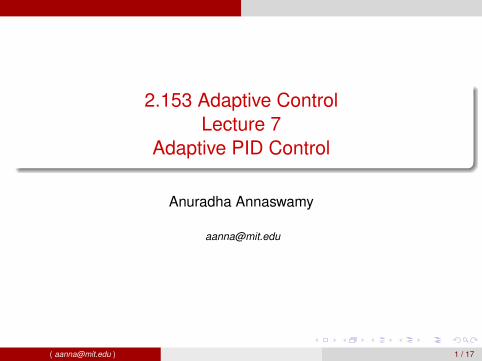
Adaptive Control of a Second-order Plant
Gc(s)1
s(Js + B)+ e τ x
−
Plant: Jx + Bx = τ J > 0
PI Control: Gc(s) = kp +ki
sτ = kpe(t) + ki
∫e(τ)dτ
Adaptive PI Control: τ = kp(t)e(t) + ki(t)∫
e(τ)dτ
PID Control: Gc(s) = kp + kds + kis
τ = kpe(t) + ki∫
e(τ)dτ + kddedt
Adaptive PID Control: τ = kp(t)e(t) + ki(t)∫
e(τ)dτ + kd(t)e(t)
J and B are unknown. Adjust kp(t), ki(t) and kd(t) so that theclosed-loop system is stable and limt→∞ e(t) = 0.
( [email protected] ) 3 / 17
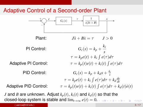
Adaptive Control of a Second-order Plant
AdaptiveController
1s(Js + B)
+ e τ x
−
Plant: Jx + Bx = τ J > 0
PI Control: Gc(s) = kp +ki
sτ = kpe(t) + ki
∫e(τ)dτ
Adaptive PI Control: τ = kp(t)e(t) + ki(t)∫
e(τ)dτ
PID Control: Gc(s) = kp + kds + kis
τ = kpe(t) + ki∫
e(τ)dτ + kddedt
Adaptive PID Control: τ = kp(t)e(t) + ki(t)∫
e(τ)dτ + kd(t)e(t)
J and B are unknown. Adjust kp(t), ki(t) and kd(t) so that theclosed-loop system is stable and limt→∞ e(t) = 0.
( [email protected] ) 3 / 17

PID -Control: Algebraic Part
NominalController
1s(Js+B)
r + er τ x
−
Gc(s) = kp +ki
s+ kds Parameterize kd = K, kp = 2λK > 0, ki = λ2K > 0
Closed-loop transfer function:K(s + λ)2
s2(Js + B) + K(s + λ)2
=K(s + λ)2
Js3 + s2(B + K) + 2Kλ2s + Kλ
Stable if0 < K <
Jλ2− B.
Design the controller so that x→ xd
( [email protected] ) 4 / 17
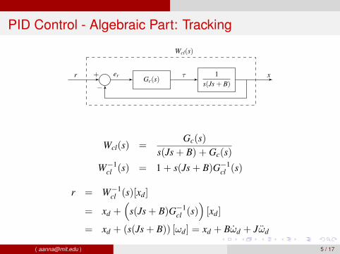
PID Control - Algebraic Part: Tracking
Gc(s)1
s(Js + B)r + er τ x
−
Wcl(s)
Wcl(s) =Gc(s)
s(Js + B) + Gc(s)
W−1cl (s) = 1 + s(Js + B)G−1
cl (s)
r = W−1cl (s)[xd]
= xd +(
s(Js + B)G−1cl (s)
)[xd]
= xd + (s(Js + B)) [ωd] = xd + Bωd + Jωd
( [email protected] ) 5 / 17

PID Control - Algebraic Part: Tracking
Gc(s)1
s(Js + B)r + er τ x
−
Wcl(s)
Wcl(s) =Gc(s)
s(Js + B) + Gc(s)
W−1cl (s) = 1 + s(Js + B)G−1
cl (s)
r = W−1cl (s)[xd]
= xd +(
s(Js + B)G−1cl (s)
)[xd]
= xd + (s(Js + B)) [ωd] = xd + Bωd + Jωd
( [email protected] ) 5 / 17
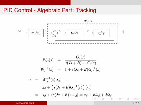
PID Control - Algebraic Part: Tracking
W−1cl (s) Gc(s)
1s(Js+B)
τxd r + er x
−
Wcl(s)
Wcl(s) =Gc(s)
s(Js + B) + Gc(s)
W−1cl (s) = 1 + s(Js + B)G−1
cl (s)
r = W−1cl (s)[xd]
= xd +(
s(Js + B)G−1cl (s)
)[xd]
= xd + (s(Js + B)) [ωd] = xd + Bωd + Jωd
( [email protected] ) 5 / 17
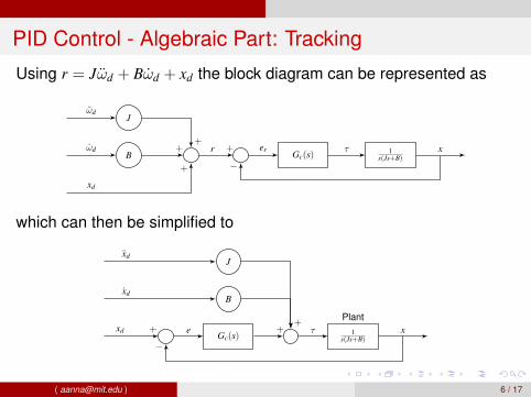
PID Control - Algebraic Part: Tracking
Using r = Jωd + Bωd + xd the block diagram can be represented as
J
B Gc(s)1
s(Js+B)
ωd
ωd
xd
+
++ r + er τ x
−
which can then be simplified to
Gc(s)
B
J
1s(Js+B)
Plantxd +
xd
xd
+e + τ x
−
( [email protected] ) 6 / 17

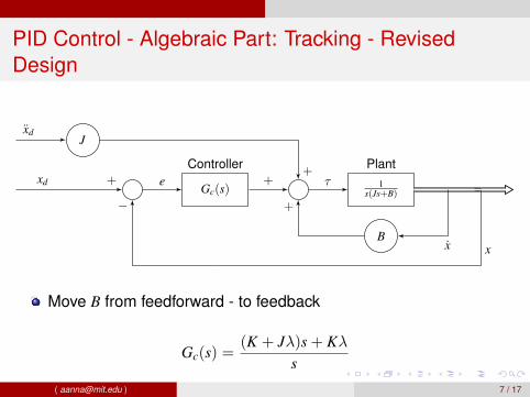
PID Control - Algebraic Part: Tracking - RevisedDesign
Gc(s)
B
J
1s(Js+B)
Plantxd +
xd
xd
+e + τ x
−
Move B from feedforward - to feedback
Gc(s) =(K + Jλ)s + Kλ
s
( [email protected] ) 7 / 17
PID Control - Algebraic Part: Tracking - RevisedDesign
J
Gc(s)
Controller1
s(Js+B)
Plant
B
xd +
xd
+e + τ
x
+
x
−
Move B from feedforward - to feedback
Gc(s) =(K + Jλ)s + Kλ
s
( [email protected] ) 7 / 17

PID Control - Algebraic Part: Tracking - RevisedDesign
Gc(s)1
s(Js + B)
B
r + er + τ
x
+
x
−
Reparameterize to accommodate J:
Gc(s) =(K + 2λJ)s2 + (2λK + λ2J)s + λ2K
s
Wcl(s) =(K + 2λJ)s2 + (2λK + λ2J)s + λ2K
Js3 + (K + 2λJ)s2 + (2λK + λ2J)s + λ2K
Always stable, for any J and B.( [email protected] ) 8 / 17
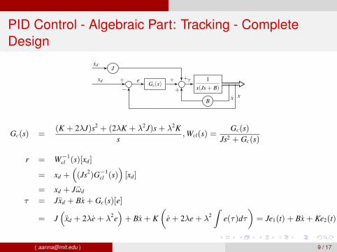
PID Control - Algebraic Part: Tracking - CompleteDesign
J
Gc(s)1
s(Js + B)
B
xd +
xd
+e + τ
x+
x−
Gc(s) =(K + 2λJ)s2 + (2λK + λ2J)s + λ2K
s,Wcl(s) =
Gc(s)Js2 + Gc(s)
r = W−1cl (s)[xd]
= xd +((Js2)G−1
cl (s))[xd]
= xd + Jωd
τ = Jxd + Bx + Gc(s)[e]
= J(
xd + 2λe + λ2e)+ Bx + K
(e + 2λe + λ2
∫e(τ)dτ
)= Je1(t) + Bx + Ke2(t)
( [email protected] ) 9 / 17

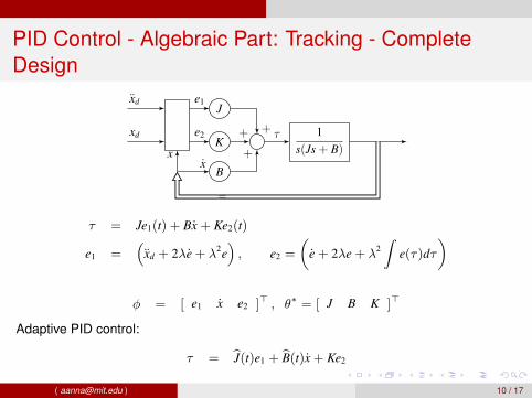
PID Control - Algebraic Part: Tracking - CompleteDesign
J
K
B
1s(Js + B)
xd
xd
e1
e2++
+
τ
xx
τ = Je1(t) + Bx + Ke2(t)
e1 =(
xd + 2λe + λ2e), e2 =
(e + 2λe + λ2
∫e(τ)dτ
)
φ = [ e1 x e2 ]> , θ∗ = [ J B K ]>
Adaptive PID control:
τ = J(t)e1 + B(t)x + Ke2
( [email protected] ) 10 / 17

PID Control - Algebraic Part: Tracking - CompleteDesign
J
K
B
1s(Js + B)
xd
xd
e1
e2++
+
τ
xx
τ = Je1(t) + Bx + Ke2(t)
e1 =(
xd + 2λe + λ2e), e2 =
(e + 2λe + λ2
∫e(τ)dτ
)
φ = [ e1 x e2 ]> , θ∗ = [ J B K ]>
Adaptive PID control:
τ = J(t)e1 + B(t)x + Ke2
( [email protected] ) 10 / 17

PID Control - Algebraic Part: Tracking - CompleteDesign
J
K
B
1s(Js + B)
xd
xd
e1
e2++
+
τ
xx
τ = Je1(t) + Bx + Ke2(t)
e1 =(
xd + 2λe + λ2e), e2 =
(e + 2λe + λ2
∫e(τ)dτ
)
φ = [ e1 x e2 ]> , θ∗ = [ J B K ]>
Adaptive PID control:
τ = J(t)e1 + B(t)x + Ke2
( [email protected] ) 10 / 17
PID Control - Algebraic Part: Tracking - CompleteDesign
J
K
B
1s(Js + B)
xd
xd
e1
e2++
+
τ
xx
τ = Je1(t) + Bx + Ke2(t)
e1 =(
xd + 2λe + λ2e), e2 =
(e + 2λe + λ2
∫e(τ)dτ
)
φ = [ e1 x e2 ]> , θ∗ = [ J B K ]>
Adaptive PID control:
τ = J(t)e1 + B(t)x + Ke2
( [email protected] ) 10 / 17

PID Control - Algebraic Part: Tracking - CompleteDesign
J
K
B
1s(Js + B)
xd
xd
e1
e2++
+
τ
xx
τ = Je1(t) + Bx + Ke2(t)
e1 =(
xd + 2λe + λ2e), e2 =
(e + 2λe + λ2
∫e(τ)dτ
)
φ = [ e1 x e2 ]> , θ∗ = [ J B K ]>
Adaptive PID control:
τ = J(t)e1 + B(t)x + Ke2
( [email protected] ) 10 / 17

PID Control - Algebraic Part: Tracking - CompleteDesign
J
K
B
1s(Js + B)
xd
xd
e1
e2++
+
τ
xx
τ = Je1(t) + Bx + Ke2(t)
e1 =(
xd + 2λe + λ2e), e2 =
(e + 2λe + λ2
∫e(τ)dτ
)
φ = [ e1 x e2 ]> , θ∗ = [ J B K ]>
Adaptive PID control:
τ = J(t)e1 + B(t)x + Ke2
( [email protected] ) 10 / 17

PID Control - Algebraic Part: Tracking - CompleteDesign
J
K
B
1s(Js + B)
xd
xd
e1
e2++
+
τ
xx
τ = Je1(t) + Bx + Ke2(t)
e1 =(
xd + 2λe + λ2e), e2 =
(e + 2λe + λ2
∫e(τ)dτ
)
φ = [ e1 x e2 ]> , θ∗ = [ J B K ]>
Adaptive PID control:
τ = J(t)e1 + B(t)x + Ke2
( [email protected] ) 10 / 17
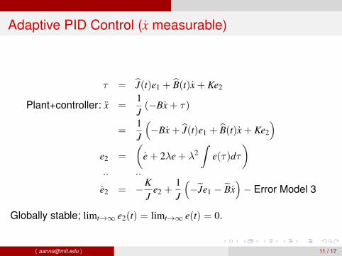
Adaptive PID Control (x measurable)
τ = J(t)e1 + B(t)x + Ke2
Plant+controller: x =1J(−Bx + τ)
=1J
(−Bx + J(t)e1 + B(t)x + Ke2
)e2 =
(e + 2λe + λ2
∫e(τ)dτ
).. ..
e2 = −KJ
e2 +1J
(−Je1 − Bx
)− Error Model 3
Globally stable; limt→∞ e2(t) = limt→∞ e(t) = 0.
( [email protected] ) 11 / 17
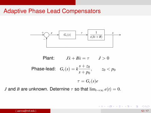
Adaptive Phase Lead Compensators
Gc(s)1
s(Js + B)+ e τ x
−
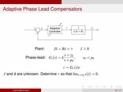
Plant: Jx + Bx = τ J > 0
Phase-lead: Gc(s) = ks + z0
s + p0, z0 < p0
τ = Gc(s)e
J and B are unknown. Deternine τ so that limt→∞ e(t) = 0.
( [email protected] ) 12 / 17

Adaptive Phase Lead Compensators
Gc(s)1
s(Js + B)+ e τ x
−
Plant: Jx + Bx = τ J > 0
Phase-lead: Gc(s) = ks + z0
s + p0, z0 < p0
τ = Gc(s)e
J and B are unknown. Deternine τ so that limt→∞ e(t) = 0.
( [email protected] ) 12 / 17

Adaptive Phase Lead Compensators
Gc(s)1
s(Js + B)+ e τ x
−
Plant: Jx + Bx = τ J > 0
Phase-lead: Gc(s) = ks + z0
s + p0, z0 < p0
τ = Gc(s)e
J and B are unknown. Deternine τ so that limt→∞ e(t) = 0.
( [email protected] ) 12 / 17
Adaptive Phase Lead Compensators
AdaptiveController
1s(Js + B)
+ e τ x
−
Plant: Jx + Bx = τ J > 0
Phase-lead: Gc(s) = ks + z0
s + p0, z0 < p0
τ = Gc(s)e
J and B are unknown. Deternine τ so that limt→∞ e(t) = 0.
( [email protected] ) 12 / 17
Phase Lead Compensators - Algebraic Part
NominalController
1s(Js+B) s + a
θ0
cmd + x, x y
−
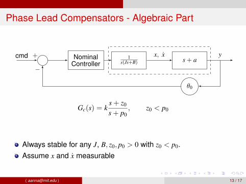
Gc(s) = ks + z0
s + p0, z0 < p0
Always stable for any J, B, z0, p0 > 0 with z0 < p0.Assume x and x measurable
( [email protected] ) 13 / 17

Phase Lead Compensators - Synthetic output y
J
B
θ0
Gc(s)1
s(Js+B) s + a
θ0
ω′d
ω′d
yd
++
+
+ v x, x y
−
Wcl(s)
ν = θ0(yd − y) + Bω′d + Jω′d
Stable for all parameters of Gc(s)
θ0 = θ∗ - value for which Wcl(s) has a desired phase margin
( [email protected] ) 14 / 17
Adaptive Phase Lead Compensators - Syntheticoutput y
J
B
θy
Gc(s)1
s(Js+B) s + a
θy
ω′d
ω′d
yd
++
+
+ v x, x y
−
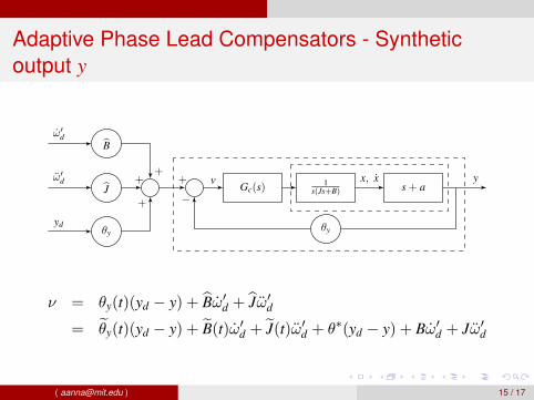
ν = θy(t)(yd − y) + Bω′d + Jω′d= θy(t)(yd − y) + B(t)ω′d + J(t)ω′d + θ∗(yd − y) + Bω′d + Jω′d
( [email protected] ) 15 / 17
Adaptive Phase Lead Compensators - Syntheticoutput y
B
J
θ∗
θ
Gc(s)1
s(Js+B) s + a
θ∗
ω′d
ω′d
yd
ω
++
+
+
+ v x, x y
−
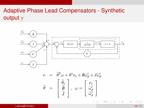
ν = θTω + θ∗ey + Bω′d + Jω′d
θ =
θy
BJ
, ω =
ey
ω′dω′d
( [email protected] ) 16 / 17
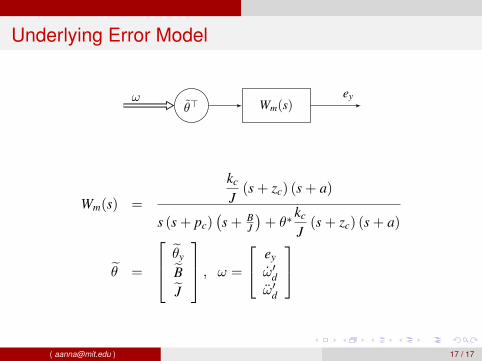
Underlying Error Model
θ> Wm(s)ω ey
Wm(s) =
kc
J(s + zc) (s + a)
s (s + pc)(s + B
J
)+ θ∗
kc
J(s + zc) (s + a)
θ =
θy
BJ
, ω =
ey
ω′dω′d
( [email protected] ) 17 / 17


![Vehicle Based on Adaptive PID Neural Network · of adaptive controllers represents a very promising technique for such uncertain and nonlinear application [19]. The neural networks](https://static.fdocuments.us/doc/165x107/5fb1b8c4f5596115e8784d83/vehicle-based-on-adaptive-pid-neural-network-of-adaptive-controllers-represents.jpg)


