2.153 Adaptive Control Lecture 1 Simple Adaptive …aaclab.mit.edu/material/lect/lecture1.pdf2.153...
39
2.153 Adaptive Control Lecture 1 Simple Adaptive Systems: Identification Anuradha Annaswamy [email protected] ( [email protected] ) 1 / 17
-
Upload
vuongkhanh -
Category
Documents
-
view
252 -
download
1
Transcript of 2.153 Adaptive Control Lecture 1 Simple Adaptive …aaclab.mit.edu/material/lect/lecture1.pdf2.153...

2.153 Adaptive ControlLecture 1
Simple Adaptive Systems: Identification
Anuradha Annaswamy
( [email protected] ) 1 / 17

Parameter Adaptation - Recursive Schemes
Adaptive Control: The control of Uncertain Systems
Adaptive Control (in this Course):The control of Linear Time-invariant Plants with Unknown Parameters
( [email protected] ) 2 / 17

Parameter Adaptation - Recursive Schemes
Adaptive Control: The control of Uncertain Systems
Adaptive Control (in this Course):The control of Linear Time-invariant Plants with Unknown Parameters
( [email protected] ) 2 / 17

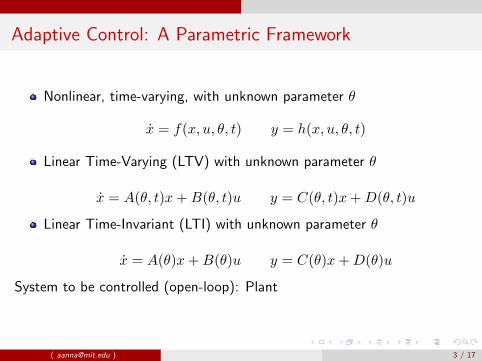
Adaptive Control: A Parametric Framework
Nonlinear, time-varying, with unknown parameter θ
x = f(x, u, θ, t) y = h(x, u, θ, t)
Linear Time-Varying (LTV) with unknown parameter θ
x = A(θ, t)x+B(θ, t)u y = C(θ, t)x+D(θ, t)u
Linear Time-Invariant (LTI) with unknown parameter θ
x = A(θ)x+B(θ)u y = C(θ)x+D(θ)u
System to be controlled (open-loop): PlantControlled System (closed-loop): System
( [email protected] ) 3 / 17
Adaptive Control: A Parametric Framework
Nonlinear, time-varying, with unknown parameter θ
x = f(x, u, θ, t) y = h(x, u, θ, t)
Linear Time-Varying (LTV) with unknown parameter θ
x = A(θ, t)x+B(θ, t)u y = C(θ, t)x+D(θ, t)u
Linear Time-Invariant (LTI) with unknown parameter θ
x = A(θ)x+B(θ)u y = C(θ)x+D(θ)u
System to be controlled (open-loop): Plant
Controlled System (closed-loop): System
( [email protected] ) 3 / 17

Adaptive Control: A Parametric Framework
Nonlinear, time-varying, with unknown parameter θ
x = f(x, u, θ, t) y = h(x, u, θ, t)
Linear Time-Varying (LTV) with unknown parameter θ
x = A(θ, t)x+B(θ, t)u y = C(θ, t)x+D(θ, t)u
Linear Time-Invariant (LTI) with unknown parameter θ
x = A(θ)x+B(θ)u y = C(θ)x+D(θ)u
System to be controlled (open-loop): PlantControlled System (closed-loop): System
( [email protected] ) 3 / 17

Direct and Indirect Adaptive Control
θp: Plant parameter - unknown; θc: Control parameter
Indirect Adaptive Control: Estimate θp as θp. Compute θc using θp.
θp → θp → θc
Direct Adaptive Control: Directly estimate θc as θc. Compute the plantestimate θp using θc
θp → θc → θc
( [email protected] ) 4 / 17

Identification of a Single Parameter
θ: Unknown, scalar
y(t) = θu(t)
Identify θ using measurements {u(t), y(t)}.
( [email protected] ) 5 / 17

Identification of a Single Parameter
θ: Unknown, scalar
y(t) = θu(t)
Identify θ using measurements {u(t), y(t)}.
( [email protected] ) 5 / 17

Identification of a Vector Parameter
y(t) = θTu(t)
y ∈ R, θ ∈ Rn, u : R+ → Rn
Identify θ using measurements {u(t), y(t)}.
( [email protected] ) 6 / 17

Identification of a Vector Parameter
y(t) = θTu(t)
y ∈ R,
θ ∈ Rn, u : R+ → Rn
Identify θ using measurements {u(t), y(t)}.
( [email protected] ) 6 / 17

Identification of a Vector Parameter
y(t) = θTu(t)
y ∈ R, θ ∈ Rn,
u : R+ → Rn
Identify θ using measurements {u(t), y(t)}.
( [email protected] ) 6 / 17

Identification of a Vector Parameter
y(t) = θTu(t)
y ∈ R, θ ∈ Rn, u : R+ → Rn
Identify θ using measurements {u(t), y(t)}.
( [email protected] ) 6 / 17

Identification of a Vector Parameter
y(t) = θTu(t)
y ∈ R, θ ∈ Rn, u : R+ → Rn
Identify θ using measurements {u(t), y(t)}.
( [email protected] ) 6 / 17

Identification of a Single Parameter - Recursive Scheme
y(t) = θu(t)
θ: Unknown, scalar
Identify θ as θ(t) at every instant
( [email protected] ) 7 / 17

Identification of a Single Parameter - Recursive Scheme
y(t) = θu(t)
θ: Unknown, scalar Identify θ as θ(t) at every instant
( [email protected] ) 7 / 17

Identification of a Vector Parameter - Recursive Scheme
y(t) = θTu(t)
y ∈ R, θ ∈ Rn, u : R+ → Rn
Identify θ as θ(t) at every instant
( [email protected] ) 8 / 17
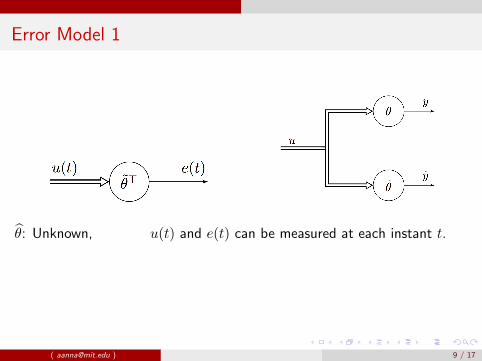
Error Model 1
θ: Unknown, u(t) and e(t) can be measured at each instant t.
( [email protected] ) 9 / 17

Identification of a Parameter in a Dynamic System
Simplest Transfer Function of a Motor:
V : Voltage input ω: Angular Velocity output
K,J,B: Physical parameters
Plant:K
Js+B=
a1s+ θ1
K,J,B unknown ⇒ a1, θ1 unknown
( [email protected] ) 10 / 17

Identification of a Parameter in a Dynamic System
Simplest Transfer Function of a Motor:
V : Voltage input ω: Angular Velocity output
K,J,B: Physical parameters
Plant:K
Js+B=
a1s+ θ1
K,J,B unknown ⇒ a1, θ1 unknown
( [email protected] ) 10 / 17

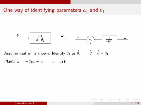
One way of identifying parameters a1 and θ1
Assume that a1 is known.
Identify θ1 as θ. θ = θ − θ1
Plant: ω = −θ1ω + u u = a1V
( [email protected] ) 11 / 17

One way of identifying parameters a1 and θ1
Assume that a1 is known. Identify θ1 as θ.
θ = θ − θ1
Plant: ω = −θ1ω + u u = a1V
( [email protected] ) 11 / 17
One way of identifying parameters a1 and θ1
Assume that a1 is known. Identify θ1 as θ. θ = θ − θ1
Plant: ω = −θ1ω + u u = a1V
( [email protected] ) 11 / 17

An alternate procedure for identifying θ1:
a1s+ θ1
=
a1s+ θm
1 +θm − θ1s+ θm
θ ≡ θ1 − θm
( [email protected] ) 13 / 17

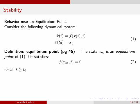
Stability
Behavior near an Equilirbium Point.
Consider the following dynamical system
x(t) = f(x(t), t)
x(t0) = x0(1)
Definition: equilibrium point (pg 45) The state xeq is an equilibriumpoint of (1) if it satisfies:
f(xeq, t) = 0 (2)
for all t ≥ t0.
( [email protected] ) 14 / 17
Stability
Behavior near an Equilirbium Point.Consider the following dynamical system
x(t) = f(x(t), t)
x(t0) = x0(1)
Definition: equilibrium point (pg 45) The state xeq is an equilibriumpoint of (1) if it satisfies:
f(xeq, t) = 0 (2)
for all t ≥ t0.
( [email protected] ) 14 / 17

Stability of LTI Plants
A motivating example: determine the stability of the origin for thefollowing scalar system
x(t) = Ax(t)
Equilibrium point: x = 0
Can determine the stability of the origin by evaluating eigenvalues of A
x(t) = eA(t−t0)x(t0)
A = V ΛV −1; V : from eigenvector; Λ : diag(λi) : from eigenvalues
Stability follows if Re(λi) ≤ 0Asymptotic stability follows if Re(λi) < 0.
Lyapunov’s methods allow us to determine the stability of an equilibriumfor such a system without solving the differential equation!
( [email protected] ) 15 / 17

Stability of LTI Plants
A motivating example: determine the stability of the origin for thefollowing scalar system
x(t) = Ax(t)
Equilibrium point: x = 0Can determine the stability of the origin by evaluating eigenvalues of A
x(t) = eA(t−t0)x(t0)
A = V ΛV −1; V : from eigenvector; Λ : diag(λi) : from eigenvalues
Stability follows if Re(λi) ≤ 0Asymptotic stability follows if Re(λi) < 0.
Lyapunov’s methods allow us to determine the stability of an equilibriumfor such a system without solving the differential equation!
( [email protected] ) 15 / 17

Lyapunov Stability
For the systemx = f(x)
Let
(i) V (x) > 0, ∀x 6= 0, and V (0) = 0
(ii) V (x) =(∂V∂x
)Tf(x) < 0
(ii) V (x)→∞ as ‖x‖ → ∞
Then x = 0 is asymptotically stable.
If instead of (ii), we have
(ii’) V ≤ 0
Then x = 0 is stable.
( [email protected] ) 16 / 17

Lyapunov Stability
For the systemx = f(x)
Let
(i) V (x) > 0, ∀x 6= 0, and V (0) = 0
(ii) V (x) =(∂V∂x
)Tf(x) < 0
(ii) V (x)→∞ as ‖x‖ → ∞
Then x = 0 is asymptotically stable.
If instead of (ii), we have
(ii’) V ≤ 0
Then x = 0 is stable.
( [email protected] ) 16 / 17

Error Model 1
Error Model 1 leads to the following
x(t) = A(t)x(t) A(t) = −u(t)uT (t)
Equilibrium point: x = 0
Choose a quadratic function
V =1
2xTx
V = xTA(t)x = −xTu(t)uT (t)x = −(xTu(t)
)2 ≤ 0
⇒ stability.A later lecture will show that if u(t) is ” persistently exciting”, x(t)→ 0.We therefore conclude that error model 1 leads to a stable parameterestimation. Asymptotic stability will be shown later.
( [email protected] ) 17 / 17

Error Model 1
Error Model 1 leads to the following
x(t) = A(t)x(t) A(t) = −u(t)uT (t)
Equilibrium point: x = 0Choose a quadratic function
V =1
2xTx
V = xTA(t)x = −xTu(t)uT (t)x = −(xTu(t)
)2 ≤ 0
⇒ stability.
A later lecture will show that if u(t) is ” persistently exciting”, x(t)→ 0.We therefore conclude that error model 1 leads to a stable parameterestimation. Asymptotic stability will be shown later.
( [email protected] ) 17 / 17

Error Model 1
Error Model 1 leads to the following
x(t) = A(t)x(t) A(t) = −u(t)uT (t)
Equilibrium point: x = 0Choose a quadratic function
V =1
2xTx
V = xTA(t)x = −xTu(t)uT (t)x = −(xTu(t)
)2 ≤ 0
⇒ stability.A later lecture will show that if u(t) is ” persistently exciting”, x(t)→ 0.
We therefore conclude that error model 1 leads to a stable parameterestimation. Asymptotic stability will be shown later.
( [email protected] ) 17 / 17

Error Model 1
Error Model 1 leads to the following
x(t) = A(t)x(t) A(t) = −u(t)uT (t)
Equilibrium point: x = 0Choose a quadratic function
V =1
2xTx
V = xTA(t)x = −xTu(t)uT (t)x = −(xTu(t)
)2 ≤ 0
⇒ stability.A later lecture will show that if u(t) is ” persistently exciting”, x(t)→ 0.We therefore conclude that error model 1 leads to a stable parameterestimation. Asymptotic stability will be shown later.
( [email protected] ) 17 / 17