2045 Long Range Transportation Plan (LRTP)

MODEL DOCUMENTATION AND APPENDIX

Mobile Area Transportation Study (MATS) Metropolitan Planning Organization (MPO)

Long Range Transportation Plan (LRTP)

Adopted: April 22, 2020

Prepared by the South

Alabama Regional Planning Commission (SARPC) 110 Beauregard St., Ste 207

Mobile, AL 36602

i

2045 Long Range Transportation Plan (LRTP)

Model Documentation and Appendix

Prepared for the Mobile Area Transportation Study (MATS) Metropolitan Planning Organization (MPO) by the South Alabama Regional

Planning Commission (SARPC)

This document is posted at

https://www.envision2045.org/

For further information, please contact Kevin Harrison, PTP, Director, Transportation Planning South Alabama Regional Planning Commission (SARPC)

110 Beauregard St., Ste 207 Mobile, AL 36602 Email: kharrison@sarpc.org

Date adopted: April 22, 2020 Date amended:

This 2045 Long Range Transportation Plan has been financed in part by the U. S. Department of Transportation, Federal Highway Administration, Federal Transit Administration, and local governments, and produced by the South Alabama Regional Planning Commission (SARPC), pursuant to requirements of amended Title 23, USC 134and 135, (as amended by the FAST ACT Sections 1201, 1202 July 2012) and Task 3.6.1 of the FY 2020 Mobile MPO Unified Planning Work Program. The contents of this document do not necessarily reflect the official views or policies of the U.S. Department of Transportation.

ii

MOBILE AREA TRANSPORTATION STUDY (MATS)

METROPOLITAN PLANNING ORGANIZATION (MPO)

MPO and Advisory Committee Officers

Fiscal Year 2020

Mobile Metropolitan Planning Organization (MPO) Hon. William S. Stimpson, Chairman, Mayor, City of Mobile

Technical Coordinating Committee / Citizens Advisory Committee (TCC/CAC)

, Chairman, Executive Director, SARPC

South Alabama Regional Planning Commission (SARPC)

Serving as staff to the MPO

, Executive Director Mr. Kevin

Harrison, Transportation Planning Director Mr. Thomas Piper,

Senior Transportation Planner

Ms. Monica Williamson, Transportation Planner Mr.

Anthony Johnson, Transportation Planner

Fiscal Year 2020

Metropolitan Planning Organization (MPO)

Mayor, City of Mobile - Hon. William S. Stimpson (MPO Chairman)

Mobile County Commissioner - Hon. Jerry Carl

Mobile County Engineer - Mr. Bryan Kegley

Councilman, City of Mobile - Hon. John Williams

Councilman, City of Mobile - Hon. Fred Richardson

Mayor, City of Prichard - Hon. Jimmie Gardner

Councilman, City of Prichard - Hon. Lorenzo Martin

Mayor, City of Chickasaw - Hon. Byron Pittman

Mayor, City of Saraland - Hon. Howard Rubenstein

Mayor, City of Satsuma - Hon. Thomas Williams

Mayor, City of Creola - Hon. William Criswell

Mayor, City of Bayou La Batre Hon. Terry Downey

Mayor, City of Semmes Hon. David Baker

General Manager, the Wave Transit System, Mr. Damon Dash

Southwest Region Engineer, ALDOT - Mr. Matt Ericksen

Member, SARPC Mr. Robert Middleton

Bureau Chief, Local Transportation, ALDOT (Non-voting) Division

iii

Administrator, FHWA (Non-voting) - Mr. Mark Bartlett

Executive Director, SARPC (Non-voting) -

Metropolitan Planning Organization Joint Technical / Citizens Advisory

Committee Members

Alabama State Docks - Mr. Bob Harris

At Large - Mr. John Blanton

Citizen - Mr. Donald Watson

Citizen - Mr. John Murphy

Citizen - Mr. Merrill Thomas

City of Bayou La Batre - Mr. Frank Williams

City of Chickasaw - Mr. Dennis Sullivan

City of Mobile - Mr. Nick Amberger

City of Mobile - Ms. Shayla Beaco

City of Mobile - Ms. Mary Beth Bergin

City of Mobile - Mr. James DeLapp

City of Mobile - Ms. Jennifer White

City of Prichard - Mr. Essie Johnson

City of Prichard - Mr. Fernando Billups

City of Prichard - Mr. James Jacobs

City of Saraland – Mr. Logan Anderson

City of Saraland – Ms. Shilo Miller

City of Satsuma - Mr. Tom Briand

Freight - Mr. Brian Harold

At-Large - Mr. Jeff Zoghby

Mobile Airport Authority - Mr. Jason Wilson

Mobile Area Chamber of Commerce - Ms. Nancy Hewston

Mobile Bay Keeper - Ms. Casi Callaway Mobile County - Mr. Ricky Mitchell

Mobile County - Ms. Kim Sanderson

Mobile County - Mr. Richard Spraggins

Mobile County Health Dept. - Dr. Ted Flotte

Mobile United, Executive Director - Ms. Christienne Gibson

Partners for Environmental Progress - Ms. Jennifer Denson

Private Transit Provider - Vacant

SARPC -

The Wave Transit System - Mr. Gerald Alfred

iv

Mobile Area Transportation Study

Metropolitan Planning Organization Bicycle / Pedestrian Advisory Committee

Members

John Blanton, Mobile Bike Club Urban Assault (BPAC Chairperson)

Edwin Perry, Alabama Department of Transportation, Southwest Region

Daniel Driskell, Alabama Department of Transportation, Southwest Region

Daniel Otto, City of Mobile Parks and Recreation Department

Jennifer White, City of Mobile Traffic Engineering

Marybeth Bergin, City of Mobile Traffic Engineering

Butch Ladner, City of Mobile Traffic Engineering

Jennifer Green, City of Mobile

Bill Finch, Cyclist

Fred Rendfrey, Downtown Mobile Alliance

Carol Hunter, Downtown Mobile Alliance (BPAC Vice-Chairperson)

Ted Flotte, Health Department, Mobilians on Bikes

Richard Spraggins, Mobile County Engineering

Timothy Wicker, Mobile County Engineering

James Foster, Mobile County Engineering

Ashley Dukes, Midtown Mobile Movement

Stephanie Woods-Crawford, Mobile County Health Department

Meredith Driskin, Mobile Baykeeper

Green Suttles, Mobile United

Dorothy Dorton, AARP

Dr. Raoul Richardson, Citizen

Ben Brenner, Mobilians on Bikes

Mark Berte, Alabama Coastal Foundation/ Livable Communities Coalition

Allison Reese, City of Satsuma

Debi Foster, The Peninsula of Mobile

Linda St. John, the Village of Springhill

v

MATS Model Documentation Appendix A

Appendix A Table of Contents

2045 Long Range Transportation Plan (LRTP) .................................................................................................................. i

Model Documentation and Appendix ............................................................................................................................. i

MPO and Advisory Committee Officers .......................................................................................................................... ii

Metropolitan Planning Organization Joint Technical / Citizens Advisory Committee Members ................... iii

Mobile Area Transportation Study ........................................................................................................................... iv

Metropolitan Planning Organization Bicycle / Pedestrian Advisory Committee Members ............................ iv

Appendix A Table of Contents ............................................................................................................................................ v

PREFACE .............................................................................................................................................................................. 1

Appendix A TRAVEL MODEL INPUT ..................................................................................................................................... 2

SECTION 2 MODEL DEVELOPMENT AND VALIDATION ................................................................................................. 14

2.1 Network Development ........................................................................................................................................ 14

SECTION 3 TRIP GENERATION ...................................................................................................................................... 24

SECTION 4 TRUCKS ....................................................................................................................................................... 29

SECTION 5 TRIP DISTRIBUTION ..................................................................................................................................... 30

5.1 Preloading ........................................................................................................................................................... 33

SECTION 6 TRAFFIC ASSINGMENT AND MODEL VALIDATION ...................................................................................... 36

6.1 Traffic Counts ...................................................................................................................................................... 36

Appendix A2 2015 Socio-Economic Data .......................................................................................................................... 48

Appendix A3 2045 Socio-economic Data .......................................................................................................................... 56

Appendix A4 2015 Trip Ends ............................................................................................................................................. 64

Appendix A5 2045 Trip Ends ............................................................................................................................................. 72

Appendix A6 MATS Link Codes, Capacities, and Coded Speeds ....................................................................................... 80

Appendix A7 Friction Factors ............................................................................................................................................ 83

Appendix A8 Screenline Error ........................................................................................................................................... 87

Appendix A9 Trucks .......................................................................................................................................................... 94

APPENDIX A-10 ................................................................................................................................................................... 99

1.0 INTRODUCTION ..................................................................................................................................................... 100

2.0 AIRSAGE TECHNOLOGY ......................................................................................................................................... 100

vi

3.0 AIRSAGE STUDY METHODOLOGY ......................................................................................................................... 101

3.1 ANALYSIS COMPONENTS ...................................................................................................................................... 102

3.1.1 Data Output .................................................................................................................................................... 103

3.1.2 Subscriber Visibility ........................................................................................................................................ 103

3.1.3 Subscriber Home & Work Assignments .......................................................................................................... 103

3.2 TAZ (Traffic Analysis Zone) Assignment ............................................................................................................... 103

3.2.1 Overview ....................................................................................................................................................... 103

3.3 Data Expansion ..................................................................................................................................................... 104

3.4 Post-Processing ................................................................................................................................................... 104

4.0 PROJECT SPECIFICS ............................................................................................................................................... 104

TECHNICAL MEMORANDUM ....................................................................................................................................... 105

Appendix A – Friction Factors .................................................................................................................................. 114

Appendix A11 S.L.U.E.T.H. Methodology ....................................................................................................................... 117

Step 1: Data Set Preparation....................................................................................................................................... 118

Step 2: Download and verify model functions ............................................................................................................ 125

Step 3: Calibration ....................................................................................................................................................... 128

Step 4: Selecting Coefficient Ranges ........................................................................................................................... 134

Step 5: Model Prediction ............................................................................................................................................ 136

Step 6: Determine the Percent Urban Change for Each TAZ ...................................................................................... 140

Appendix A12 2015-2045 Volume Plots ..................................................................................................................... 143

Figures Figure 1 Comparison of Vehicle Ownership by Income Data ............................................................................................. 4 Figure 2 MATS Traffic Zones ............................................................................................................................................. 6 Figure 3 November, 2013 Cell Phone Captures .................................................................................................................. 9 Figure 4 July, 2014 Cell Phone Captures ....................................................................................................................... 9 Figure 5 MATS Planning Districts .................................................................................................................................... 10 Figure 6 Functional Classification and Mobility vs Access ............................................................................................... 15 Figure 7 Mobile Urban Area Functional Classification ..................................................................................................... 16 Figure 8 MATS 2015 Land Use Indices ............................................................................................................................ 19 Figure 9 MATS 2045 Land Use Indices ............................................................................................................................ 20 Figure 10 Streetlight Heavy Trucks Monitoring Locations ................................................................................................ 29 Figure 11 HBW Trip Length Frequency Distribution Curve ............................................................................................ 31 Figure 12 HBO Trip Length Frequency Distribution Curve ............................................................................................. 31 Figure 13 NHB Trip Length Frequency Distribution Curve .............................................................................................. 32 Figure 14 MATS 2015 Through Trips .............................................................................................................................. 34 Figure 15 MATS 2015 Truck Trips .................................................................................................................................. 35 Figure 16 Network Screenlines and Cutlines .................................................................................................................... 39

vii

Figure 17 2015 All-or-Nothing Assig nment Screenline Error .......................................................................................... 40 Figure 18 MATS Volume-Delay Curves .......................................................................................................................... 41 Figure 19 2015 Capacity Restrained Assignment Screenline Error ................................................................................... 42 Figure 20 2015 Assignment Error, By Link ...................................................................................................................... 45 Figure 21 Summary Comparisons: Model vs 2015 Conditions, Including Estimated Counts ........................................... 45 Figure A9- 1 Freight Analysis Zones 95 Figure A12- 1 2015 Volume 144 Figure A12- 2 2015 Volume/Capacity ............................................................................................................................ 145 Figure A12- 3 2045 E+C Volumes ................................................................................................................................. 146 Figure A12- 4 .................................................................................................................................................................. 147 Figure A12- 5 2045 Plan Volume ................................................................................................................................... 148

Tables Table 1 MATS Percent Households By Vehicles/HH By Income and Household Income Distribution ............................. 3 Table 2 2015 Census Percent Households By Vehicles/HH By Income and Household Income Distribution ............... 3 Table 3 Vehicle-Trip Rates By Vehicles/HH By Income (Derived from NCHRP 365) ...................................................... 4 Table 4 ALDOTs Annual Growth Rate for Future Externals .............................................................................................. 8 Table 5 Socio-Economic Data by Planning Area, 2015 - 2045 ......................................................................................... 11 Table 6 MATS Daily Trip-Ends (2015 & 2045) ............................................................................................................... 12 Table 7 MATS Link Group 1 Codes ................................................................................................................................. 17 Table 8 MATS Network Assumptions .............................................................................................................................. 21 Table 9 MATS Basic Roadway Capacity .......................................................................................................................... 23 Table 10 Average Vehicle-Trips per Household ............................................................................................................... 24 Table 11External Trip Productions and Attractions, 2015 ................................................................................................. 26 Table 12 MATS External Trip-End Summary, 2015 ......................................................................................................... 28 Table 13 Internal Trip-End Data, 2015 ............................................................................................................................. 30 Table 14 Average Trip Length .......................................................................................................................................... 32 Table 15 Distribution of 2015 Traffic Counts ................................................................................................................... 37 Table 16 2015 All-or-Nothing Assignment VMT ............................................................................................................. 38 Table 17 2015 Assignment Error by Functional Classification ......................................................................................... 42 Table 18 Comparison of Average and RMS Error by Functional Classification ............................................................... 43 Table 19 2015 Assignment RMS Error by ADT Group .................................................................................................... 44 Table 20 Summary Comparisons: Model vs 2015 Conditions, Including Estimated Counts ............................................ 46 Table 9- 1 TAZs contained within FAZs 96 Table 9- 2 2015 External Trucks and Vehicles ................................................................................................................. 97 Table 9- 3 2045 External Trucks ...................................................................................................................................... 97 Table 9- 4 Streetlight Traffic Index to Create Matrix ....................................................................................................... 98

1

PREFACE

This Mobile Area Transportation Study (MATS) Long-Range Transportation Plan to the year 2045 was

begun in 2015 under the guidance of the Mobile Urban Area Metropolitan Planning Organization (MPO).

The study was conducted by the South Alabama Regional Planning Commission with the assistance of the

Alabama Department of Transportation, the Mobile County Engineering Department, The Wave Transit

System, and the City of Mobile Transportation, Planning, and Engineering Departments. Funding has been

provided by the U. S. Department of Transportation's Federal Highway Administration and Federal Transit

Administration, by the Mobile County Commission, and by the cities of Mobile, Prichard, Chickasaw,

Saraland, Satsuma, Creola, Bayou La Batre and Semmes.

The Destination 2045 Transportation Plan is multi-modal in scope, encompassing long-range plans for

highway, public transportation, and bicycle/pedestrian networks. Regional growth, economic development,

and accessibility within the study area along with environmental concerns necessitate that the long-range

plan addresses not only improved vehicular travel but also improvements to alternative modes. Preservation

of the existing transportation system coupled with enhancement of all modal choices will contribute to

the improvement of the overall quality of life in the region.

The MPO's objective in initiating the plan update was to identify, to the maximum extent feasible, the

multi-modal transportation improvements which will be needed in the Mobile urban area between now and

the year 2045 in order to maintain an acceptable level of mobility. Where possible, these needs were

quantified in terms of dollar costs and prioritized based on the availability of funding, the anticipated

impact of the proposed improvement, and expected development patterns and timing. The Plan is not pro-

posed as a rigid, inflexible blueprint, but rather is intended to guide decision-makers' actions within a

regional context and thus maintain system coordination across the various political boundaries which

divide the MATS area.

This document explains the technical aspects of the update process, particularly the traffic modeling and

forecasting portion. The Envision 2045 Plan itself, an Executive Summary, or fold-out maps of the

various plan elements can be obtained from the Transportation Planning staff of the South Alabama

Regional Planning Commission, P.O. Box 1665, Mobile, 36633-1665. SARPC’s telephone number is

(251)433-6541; the fax number is 433-6009; and the physical address is 110 Beauregard Street, Suite 207, 36602. SARPC maintains an internet site at http://www.sarpc.org. Any e-mail concerning this report

or the Envision 2045 Transportation Plan itself should be addressed to transportation@sarpc.org.

2

Appendix A TRAVEL

MODEL INPUT

The basic factors which determine travel characteristics in any area are residential and

commercial land use patterns, historical and projected development rates, and personal income

levels. Computer models utilize this data to develop relationships between socio-economic

factors and travel characteristics. These relationships, in turn, can be used with projected

socio-economic characteristics to simulate future trip-making. However, prior to

development of the travel simulation models, some additional information or assumption is

required. Some of this missing data is related to the physical characteristics of the trips

themselves and will be discussed in the following section (Model Development and

Validation), but some of the needed data involves the number of trips generated by the

households in the study area (internal trips) and also the number of trips into or through the

study area which are generated outside the study cordon (external trips).

Household income (and implicitly the number of automobiles owned) is a critical factor in travel

behavior. In general, for a specific household at any given income level, access to more vehicles

indicates the probability of more trips being made on a daily basis, and for any given number

of vehicles per household, an increase in income will usually mean an increase in daily vehicle

trips. In other words, the higher the income, the higher the vehicle ownership rate, and the

greater the number of vehicles per household, the higher the trip rate per household. Vehicle

ownership data by income for the MATS planning area is shown in Table 1; also shown is

the distribution of households by income range for 2015 and 2045. Four important

qualifications should be made regarding this table: (1) the distribution is based on zonal

median income, not actual income for each household, (2) the income ranges are expressed

in 2015 dollars, not current dollars, (3) the distribution of households by income is based on

2015 Census/DataStory data for the MATS planning area, and (4) vehicle ownership by income

level is based on data published in 1998 by the Transportation Research Board in NCHRP

Report 365 for all urban areas in the United States grouped by population ranges.

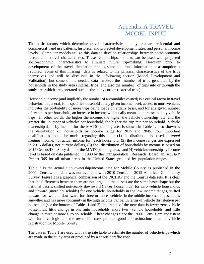
Table 2 is the actual auto ownership/income data for Mobile County as published in the

2000 Census, this data was not available with 2010 Census or 2015 American Community

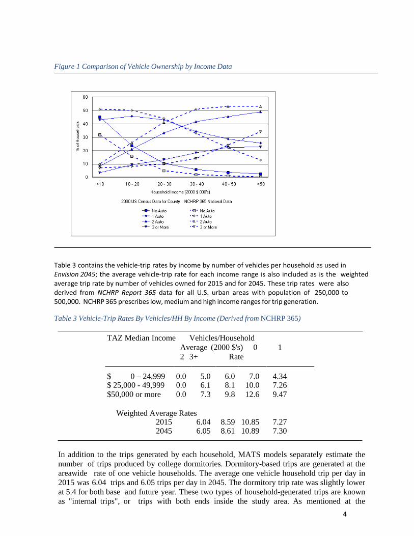
Survey. Figure 1 is a graphical comparison of the NCHRP and the Census data sets. It is clear

that the differences between them are not large — the curves are the same basic shape but the

national data is shifted noticeably downward (fewer households) for zero vehicle households

and upward (more households) for one vehicle households in the low income ranges, shifted

upward for two and downward for three or more vehicles in the middle income ranges, and is

smoother and has more continuity in the high income range. In terms of vehicle distribution per

household (see the bottom of Tables 1 and 2), the trend of the new data is fewer zero vehicle

households, little change in one auto households, more two vehicle households, and little

change in three or more auto households. These changes since the 2000 Census are consistent

with intuitive logic and the ownership rates produce good approximations of actual vehicle

registration for Mobile County.

The data in Table 1 are used with a trip rate table to estimate the number of vehicle-trips which

are made in the study area or produced by a specific traffic zone.

3

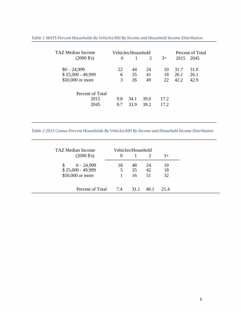
Table 1 MATS Percent Households By Vehicles/HH By Income and Household Income Distribution

TAZ Median Income

(2000 $'s) Vehicles/Household

0 1 2

3+ Percent of Total

2015 2045

$0 – 24,999 22 44 24 10 31.7 31.0 $ 25,000 - 49,999 6 35 41 18 26.1 26.1 $50,000 or more 3 26 49 22 42.2 42.9

Percent of Total 2015 9.8 34.1 39.0 17.2

2045 9.7 33.9 39.2 17.2

Table 2 2015 Census Percent Households By Vehicles/HH By Income and Household Income Distribution

TAZ Median Income

(2000 $'s)

Vehicles/Household

0 1 2

3+

$ 0 – 24,999 18 48 24 10 $ 25,000 - 49,999 5 35 42 18

$50,000 or more 1 16 51 32

Percent of Total 7.4 31.1 40.1 21.4

4

Figure 1 Comparison of Vehicle Ownership by Income Data

Table 3 contains the vehicle-trip rates by income by number of vehicles per household as used in Envision 2045; the average vehicle-trip rate for each income range is also included as is the weighted average trip rate by number of vehicles owned for 2015 and for 2045. These trip rates were also derived from NCHRP Report 365 data for all U.S. urban areas with population of 250,000 to 500,000. NCHRP 365 prescribes low, medium and high income ranges for trip generation.

Table 3 Vehicle-Trip Rates By Vehicles/HH By Income (Derived from NCHRP 365)

TAZ Median Income Vehicles/Household

Average (2000 $'s) 0 1

2 3+ Rate

$ 0 – 24,999 0.0 5.0 6.0 7.0 4.34 $ 25,000 - 49,999 0.0 6.1 8.1 10.0 7.26 $50,000 or more 0.0 7.3 9.8 12.6 9.47

Weighted Average Rates 2015 6.04 8.59 10.85 7.27 2045 6.05 8.61 10.89 7.30

In addition to the trips generated by each household, MATS models separately estimate the

number of trips produced by college dormitories. Dormitory-based trips are generated at the

areawide rate of one vehicle households. The average one vehicle household trip per day in

2015 was 6.04 trips and 6.05 trips per day in 2045. The dormitory trip rate was slightly lower

at 5.4 for both base and future year. These two types of household-generated trips are known

as "internal trips", or trips with both ends inside the study area. As mentioned at the

5

beginning of this section, the number and patterns of internal trips are determined by

household demographics and location, commercial development patterns, and employment

opportunities. These data are collected and analyzed in geographic units known as Traffic

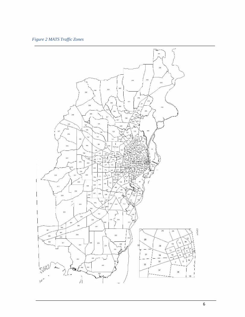
Analysis Zones (TAZ) or simply traffic zones. Figure 2 shows the current MATS zone

structure of 343 zones — 312 internal TAZ’s, 13 "dummy zones", and 18 cordon, or external,

stations. Dummy zones are not actual geographic units and therefore do not appear on

Figure 2; they are often included in model networks for ready availability to represent

future developments or possible subdivisions of TAZ's; when needed, they are moved to the

proper area of the system and "plugged in" the already developed network.

The MATS travel model uses seven independent variables to predict the trip-making

characteristics of each TAZ. Most of this information is available from standard sources such

as the U.S. Census. The necessary data includes:

• Number of households

• Zonal median household income (which includes

automobile ownership through cross

classification)

• Number of retail sector employees

• Number of service sector employees

• Number of all other nonretail sector employees

• College enrollment (enrollment at all technical

colleges, junior colleges, colleges, and/or

universities)

• Number of campus dormitory units.

6

Figure 2 MATS Traffic Zones

7

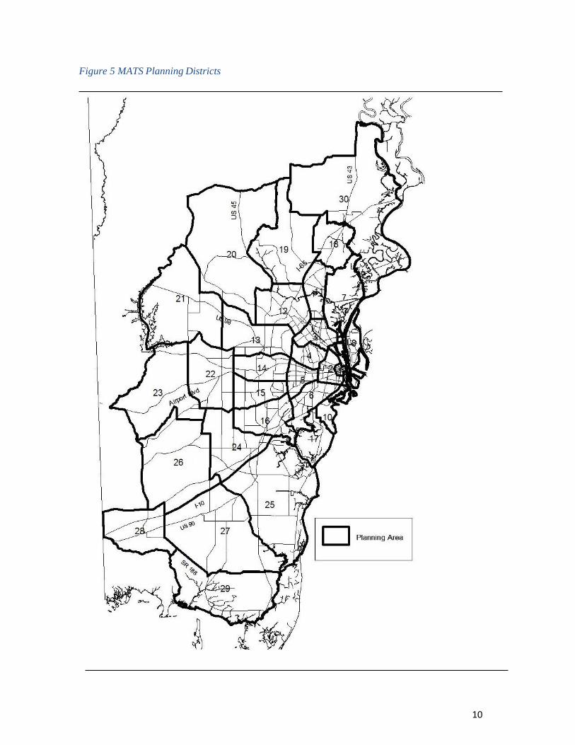
The specific TAZ data for both the base year (2015) and the forecast year (2045) are included in

Appendices 1 and 2 of this report. In order to make meaningful comparisons between different

parts of the study area without having to examine each TAZ, the internal zones are aggregated into

30 Planning Districts as illustrated in Figure 3. Table 4 shows the socio-economic data

summarized by planning district for 2015 and 2045. The next section explains how these factors

interact and influence trip-making and area travel patterns, but the product of that interaction is

shown here in Table 5, which summarizes trip-ends by planning district.

In addition to the household-generated trips, the roads in the study area will also have to provide

capacity for trips which are generated by activities outside the MATS boundary. These trips are

called external trips and can be categorized as internal-external trips or through trips. Internal-

external trips are those with one end in the study area and one end outside the study area (work

commute trips are a good example), while through trips are those with both ends outside the study

area (a vacation traveler from Louisiana on I-10 bound for Disney World is a good example of this

type). Therefore, two very different factors will affect the growth of external trips: growth and

development inside the study area and immediately adjacent areas will to a large extent dictate the

increase and pattern of internal-external trips, but factors completely unrelated to the study area

will control through trips.

Future external trips were projected using an annual growth rate applied to ALDOT external

count data obtained from ALDOT (see Table 4) called Long Growth. In percentage terms, the

resulting increase in external trips is substantially higher than the increase in internal trips. As

shown in Table 6, by 2045 internal vehicle-trip ends are projected to increase by 12%, but external

trips are projected to increase by 52%.

8

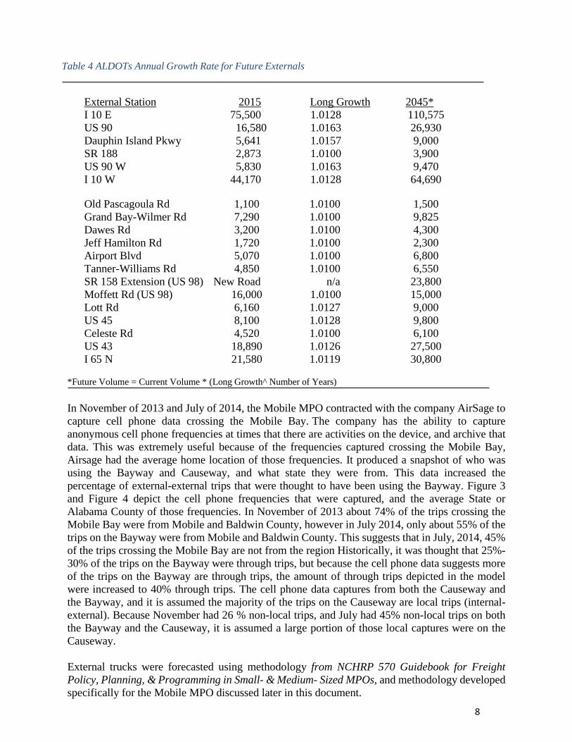
Table 4 ALDOTs Annual Growth Rate for Future Externals

External Station 2015 Long Growth 2045*

I 10 E 75,500 1.0128 110,575

US 90 16,580 1.0163

26,930

Dauphin Island Pkwy 5,641 1.0157 9,000

SR 188 2,873 1.0100 3,900

US 90 W 5,830 1.0163 9,470

I 10 W 44,170 1.0128 64,690

Old Pascagoula Rd 1,100 1.0100 1,500

Grand Bay-Wilmer Rd 7,290 1.0100 9,825

Dawes Rd 3,200 1.0100 4,300

Jeff Hamilton Rd 1,720 1.0100 2,300

Airport Blvd 5,070 1.0100 6,800

Tanner-Williams Rd 4,850 1.0100 6,550

SR 158 Extension (US 98) New Road n/a 23,800

Moffett Rd (US 98) 16,000 1.0100 15,000

Lott Rd 6,160 1.0127 9,000

US 45 8,100 1.0128 9,800

Celeste Rd 4,520 1.0100 6,100

US 43 18,890 1.0126 27,500

I 65 N 21,580 1.0119 30,800

*Future Volume = Current Volume * (Long Growth^ Number of Years)

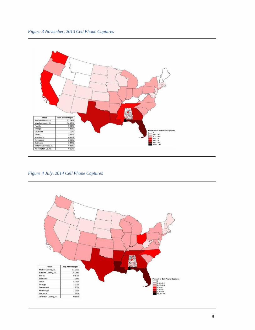
In November of 2013 and July of 2014, the Mobile MPO contracted with the company AirSage to

capture cell phone data crossing the Mobile Bay. The company has the ability to capture

anonymous cell phone frequencies at times that there are activities on the device, and archive that

data. This was extremely useful because of the frequencies captured crossing the Mobile Bay,

Airsage had the average home location of those frequencies. It produced a snapshot of who was

using the Bayway and Causeway, and what state they were from. This data increased the

percentage of external-external trips that were thought to have been using the Bayway. Figure 3

and Figure 4 depict the cell phone frequencies that were captured, and the average State or

Alabama County of those frequencies. In November of 2013 about 74% of the trips crossing the

Mobile Bay were from Mobile and Baldwin County, however in July 2014, only about 55% of the

trips on the Bayway were from Mobile and Baldwin County. This suggests that in July, 2014, 45%

of the trips crossing the Mobile Bay are not from the region Historically, it was thought that 25%-

30% of the trips on the Bayway were through trips, but because the cell phone data suggests more

of the trips on the Bayway are through trips, the amount of through trips depicted in the model

were increased to 40% through trips. The cell phone data captures from both the Causeway and

the Bayway, and it is assumed the majority of the trips on the Causeway are local trips (internal-

external). Because November had 26 % non-local trips, and July had 45% non-local trips on both

the Bayway and the Causeway, it is assumed a large portion of those local captures were on the

Causeway.

External trucks were forecasted using methodology from NCHRP 570 Guidebook for Freight

Policy, Planning, & Programming in Small- & Medium- Sized MPOs, and methodology developed

specifically for the Mobile MPO discussed later in this document.

9

Figure 3 November, 2013 Cell Phone Captures

Figure 4 July, 2014 Cell Phone Captures

10

Figure 5 MATS Planning Districts

11

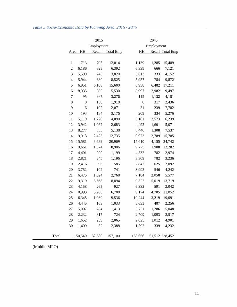
Table 5 Socio-Economic Data by Planning Area, 2015 - 2045

2015 2045

Employment Employment

Area HH Retail Total Emp HH Retail Total Emp

1 713 705 12,014 1,139 1,285 15,489

2 6,186 625 6,392 6,339 666 7,121

3 5,599 243 3,820 5,613 333 4,152

4 5,944 630 8,525 5,957 784 9,872

5 6,951 6,108 15,600 6,958 6,482 17,211

6 8,935 665 5,530 8,997 2,982 9,497

7 95 987 3,276 115 1,132 4,181

8 0 150 1,918 0 317 2,436

9 6 102 2,071 31 239 7,782

10 193 134 3,176 209 334 5,276

11 5,119 1,720 4,090 5,181 2,573 6,239

12 3,942 1,082 2,683 4,492 1,601 5,071

13 8,277 833 5,138 8,446 1,308 7,537

14 9,913 2,423 12,735 9,973 2,789 15,785

15 15,581 3,639 20,969 15,610 4,155 24,742

16 9,661 1,374 8,906 9,775 1,908 12,282

17 4,401 290 1,199 4,532 782 2,974

18 2,821 245 1,196 3,309 782 3,236

19 2,416 96 585 2,842 625 2,092

20 3,752 102 741 3,992 546 4,242

21 6,475 1,024 2,768 7,184 2,058 5,577

22 9,319 3,568 8,894 9,522 5,019 13,719

23 4,158 265 927 6,332 591 2,042

24 8,993 3,206 6,788 9,174 4,785 11,852

25 6,345 1,089 9,536 10,244 3,219 19,091

26 4,445 163 1,033 5,633 487 2,256

27 5,007 284 1,413 5,731 1,286 5,048

28 2,232 317 724 2,709 1,093 2,517

29 1,652 259 2,065 2,025 1,012 4,901

30 1,409 52 2,388 1,592 339 4,232

Total 150,540 32,380 157,100 163,656 51,512 238,452

(Mobile MPO)

12

Table 6 MATS Daily Trip-Ends (2015 & 2045)

Planning District 2015 2045 Change Percent

1 72,944 81,678 8,734 12%

2 88,985 79,970 -9,015 -10%

3 53,524 49,309 -4,215 -8%

4 93,769 86,366 -7,403 -8%

5 225,751 196,729 -29,022 -13%

6 94,004 128,197 34,193 36%

7 28,734 27,537 -1,197 -4%

8 8,771 10,734 1,963 22%

9 8,809 24,164 15,355 174%

10 16,520 22,373 5,853 35%

11 83,045 90,305 7,260 9%

12 61,444 73,380 11,936 19%

13 94,808 100,355 5,547 6%

14 233,539 227,593 -5,946 -3%

15 289,753 267,778 -21,975 -8%

16 139,402 141,449 2,047 1%

17 40,746 50,566 9,820 24%

18 30,837 45,301 14,464 47%

19 22,036 35,352 13,316 60%

20 31,952 50,991 19,039 60%

21 77,052 96,058 19,006 25%

22 168,556 182,663 14,107 8%

23 41,309 62,069 20,760 50%

24 149,992 168,398 18,406 12%

25 100,192 173,709 73,517 73%

26 40,899 54,769 13,870 34%

27 45,967 72,818 26,851 58%

28 24,743 41,995 17,252 70%

29 23,779 41,437 17,658 74%

30 19,420 27,164 7,744 40%

Total Internal 2,411,282 2,711,207 299,925 12%

External

New US 98 0 23,800 23,800 NA%

I-10 E 75,500 110,575 35,075 46%

US 90 E 16,580 26,930 10,350 62%

Dauphin Island Pkwy 5,641 9,000 3,359 60%

SR 188 2,873 3,900 1,027 36%

US 90 W 5,830 9,470 3,640 62%

I-10 W 44,170 64,690 20,520 46%

Old Pascagoula 1,100 1,500 400 36%

Grand Bay-Wilmer 7,290 9,825 2,535 35%

Dawes 3,200 4,300 1,100 34%

Jeff Hamilton 1,720 2,300 580 34%

Airport 5,070 6,800 1,730 34%

Tanner-Williams 4,850 6,550 1,700 35%

US 98 W 16,000 15,000 -1,000 -6%

Lott 6,160 9,000 2,840 46%

US 45 N 8,100 9,800 1,700 21%

Celeste 4,520 6,100 1,580 35%

13

US 43 N 18,890 27,500 8,610 46%

I-65 N 21,580 30,800 9,220 43%

Total 249,074 377,840 128,766 52%

(Mobile MPO)

14

SECTION 2 MODEL DEVELOPMENT AND VALIDATION

As mentioned at several points previously, transportation models are used to develop reliable

mathematical relationships between socio-economic data — e.g., number of households,

household size and income, number of automobiles owned or available, school enrollment, number

of people employed and the type of their employment — and trip-making. By manipulating these

relationships and comparing predicted trips with known trip patterns, an accurate method for

predicting future travel demand can be developed. The overall accuracy of this model depends

on the accuracy of trip generation (how well does the model estimate the number and kinds of trips

actually made in the area, both regionally and locally?) and the accuracy of trip distribution (how

well do the actual trip lengths compare to the model estimates and are the actual trip patterns well

duplicated, e.g., does the model accurately predict the number of screenline crossings between a

given suburban area and the CBD?). This accuracy level, in turn, is dependent on both the quality

of the input data and the relationships developed from that data and the way the model actually

assigns the estimated trips to the road system. So while good data is required to develop a good

model, it does not insure one; the model must also handle the estimated "traffic" the way that the

area's street network does.

2.1 Network Development

A model network is made up of "zones" representing trip-ends (socio-economic data), "nodes"

representing intersections, and "links" representing roadways. The trips to and from zones enter

the road system through the nodes, which are connected by links. A set of links connecting any

two zones is called a path, and a trip will always be assigned to the path with the lowest "cost"

(measured as time or distance). However, depending on how much "traffic" is already on a street

(path), the individual link costs — reflected by speed — are altered; therefore, paths can change.

The relationship of speed and traffic volume is a function of capacity.

In the real world, the capacity of a road is usually determined by the capacity of its intersections

and can be expressed as the capacity of each of the intersection approaches -- or links. This capa-

city depends on numerous factors — among them are number of through lanes, number of turn

lanes, lane width, peaking characteristics, and signalization. Of these factors, several are

categorized as physical characteristics and several as operating characteristics. Models normally

group links by both their physical and operating characteristics.

Different types of streets provide different types of service. The hierarchy of streets and roads

ordered by the type of service each provides is called "functional classification". Generally, roads

within each functional class will exhibit similar operating characteristics which will, in turn, vary

between classifications. Since operating characteristics will to a large degree determine roadway

capacity, it is extremely important that links are correctly classified in any travel model. The

15

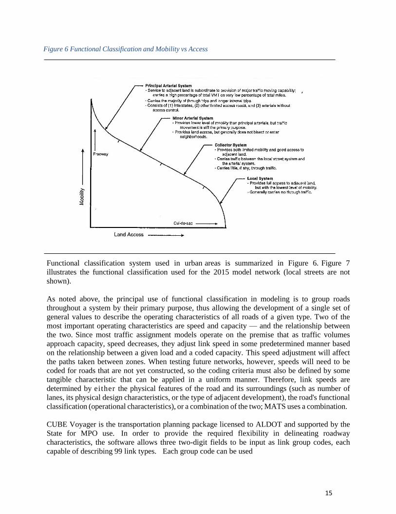
Figure 6 Functional Classification and Mobility vs Access

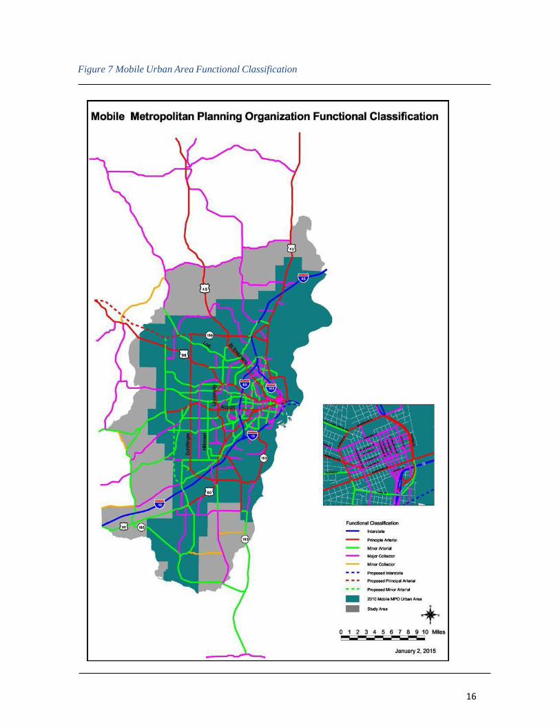
Functional classification system used in urban areas is summarized in Figure 6. Figure 7

illustrates the functional classification used for the 2015 model network (local streets are not

shown).

As noted above, the principal use of functional classification in modeling is to group roads

throughout a system by their primary purpose, thus allowing the development of a single set of

general values to describe the operating characteristics of all roads of a given type. Two of the

most important operating characteristics are speed and capacity — and the relationship between

the two. Since most traffic assignment models operate on the premise that as traffic volumes

approach capacity, speed decreases, they adjust link speed in some predetermined manner based

on the relationship between a given load and a coded capacity. This speed adjustment will affect

the paths taken between zones. When testing future networks, however, speeds will need to be

coded for roads that are not yet constructed, so the coding criteria must also be defined by some

tangible characteristic that can be applied in a uniform manner. Therefore, link speeds are

determined by either the physical features of the road and its surroundings (such as number of

lanes, its physical design characteristics, or the type of adjacent development), the road's functional

classification (operational characteristics), or a combination of the two; MATS uses a combination.

CUBE Voyager is the transportation planning package licensed to ALDOT and supported by the

State for MPO use. In order to provide the required flexibility in delineating roadway

characteristics, the software allows three two-digit fields to be input as link group codes, each

capable of describing 99 link types. Each group code can be used

16

Figure 7 Mobile Urban Area Functional Classification

17

to describe some specific aspect or group of aspects of each link (piece of road) in the system.

For example, the first link group field might be coded for a road’s functional classification, the

second for number of lanes, and the third for the type of adjacent land use. Any specific

combination of these three codes identifies a unique set of road characteristics which corresponds

to a specific speed and a specific operating capacity.

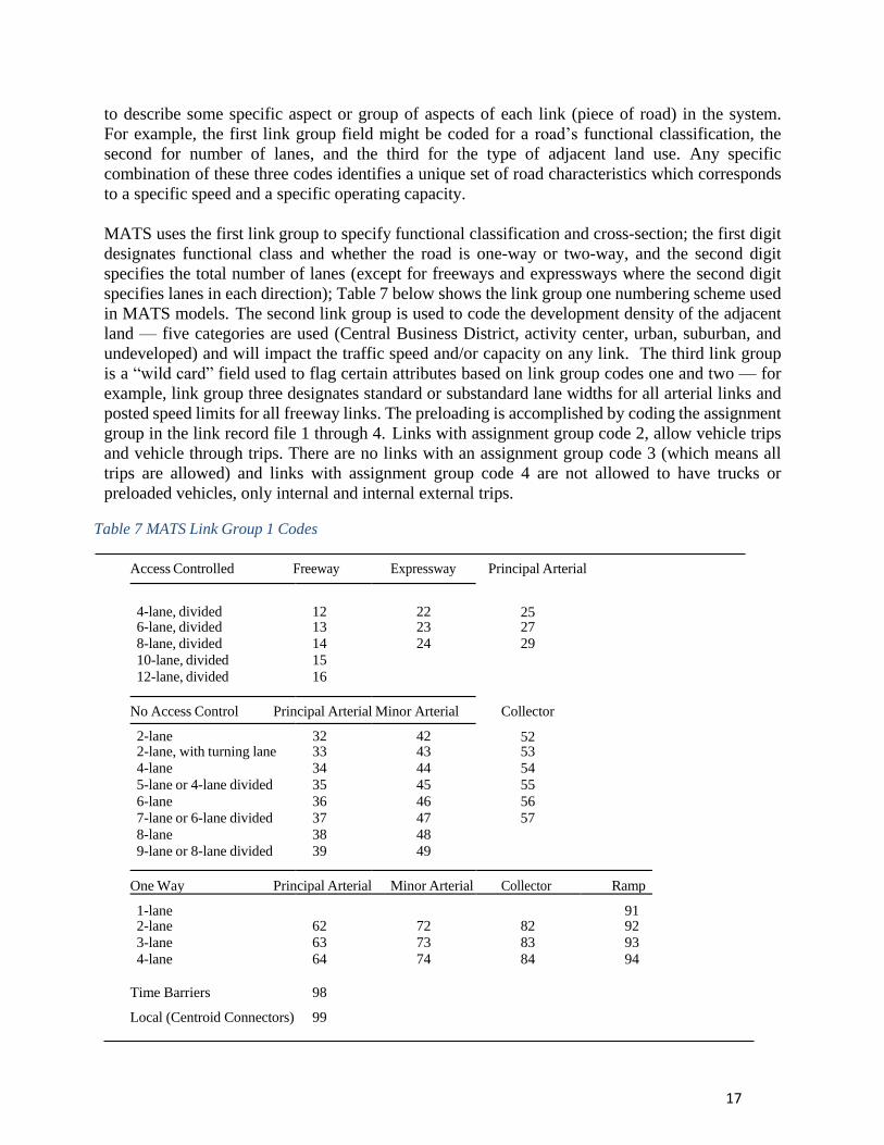
MATS uses the first link group to specify functional classification and cross-section; the first digit

designates functional class and whether the road is one-way or two-way, and the second digit

specifies the total number of lanes (except for freeways and expressways where the second digit

specifies lanes in each direction); Table 7 below shows the link group one numbering scheme used

in MATS models. The second link group is used to code the development density of the adjacent

land — five categories are used (Central Business District, activity center, urban, suburban, and

undeveloped) and will impact the traffic speed and/or capacity on any link. The third link group

is a “wild card” field used to flag certain attributes based on link group codes one and two — for

example, link group three designates standard or substandard lane widths for all arterial links and

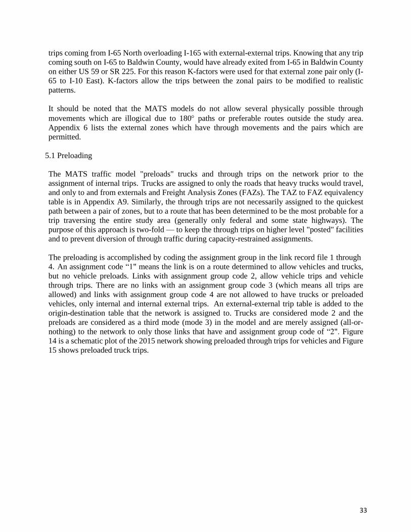
posted speed limits for all freeway links. The preloading is accomplished by coding the assignment

group in the link record file 1 through 4. Links with assignment group code 2, allow vehicle trips

and vehicle through trips. There are no links with an assignment group code 3 (which means all

trips are allowed) and links with assignment group code 4 are not allowed to have trucks or

preloaded vehicles, only internal and internal external trips.

Table 7 MATS Link Group 1 Codes

Access Controlled Freeway Expressway Principal Arterial

4-lane, divided

12

22

25

6-lane, divided 13 23 27

8-lane, divided 14 24 29

10-lane, divided 15 12-lane, divided 16

No Access Control Principal Arterial Minor Arterial Collector

2-lane 32 42 52 2-lane, with turning lane 33 43 53

4-lane 34 44 54

5-lane or 4-lane divided 35 45 55

6-lane 36 46 56

7-lane or 6-lane divided 37 47 57

8-lane 38 48 9-lane or 8-lane divided 39 49

One Way Principal Arterial Minor Arterial Collector Ramp

1-lane 91 2-lane 62 72 82 92

3-lane 63 73 83 93

4-lane 64 74 84 94

Time Barriers 98

Local (Centroid Connectors) 99

18

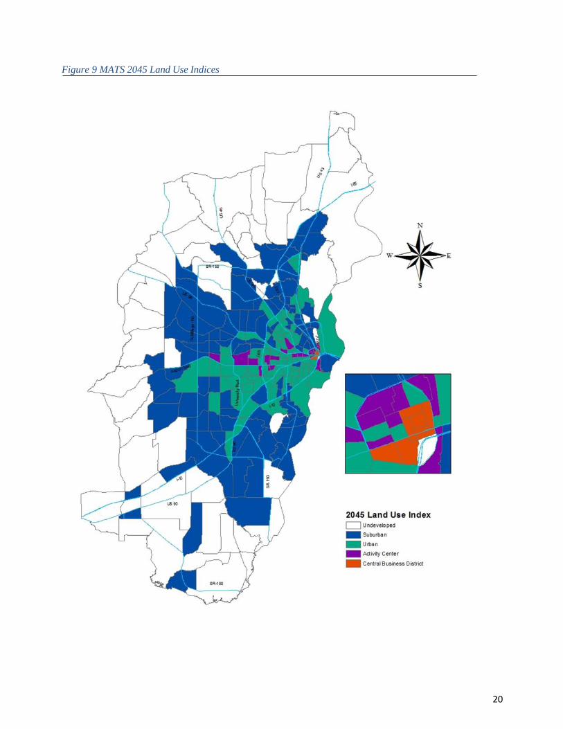
Land use and development density are extremely important criteria in model validation since they

impact both the speed and capacity of a road network. As noted above, the link group two field

is used to indicate one of five land use densities. These densities will change over time, of course,

so this factor will have variable impacts on the traffic model as study area conditions change. In

addition to network link speeds and capacities, changes in the development density will impact

terminal times (the elapsed time between leaving the public road system and entering the

destination) and intrazonal times (the time required to complete a trip within a single zone without

leaving the local road system). Since future development will change the current patterns, it is

important to develop a quantitative methodology or index that will allow known or projected

factors (i.e., socio-economic data) to represent future development conditions. In this way, a

more accurate scenario of the impact of specific development on future road systems will be

achieved. This is accomplished in the MATS models through the use of an “Activity Index”

which quantifies development in terms of its density (units per acre) by traffic zone.

In the MATS application, no determination was made regarding the relative impacts of commercial

versus residential development; similarly, no distinction has been made between retail and other

employment types. The index is calculated by simply adding households, college dormitory units,

total employment, and post-secondary education enrollment and then dividing the total by the size

of the traffic zone in acres. The break points between land development types were determined

based on base year conditions and the relationship of the calculated densities to known

development levels; large gaps in the series of calculated densities were also utilized to stratify the

levels. The break points are then fixed, and future development scenarios are evaluated based on

the calculated future index, with the necessary and appropriate adjustments made throughout the

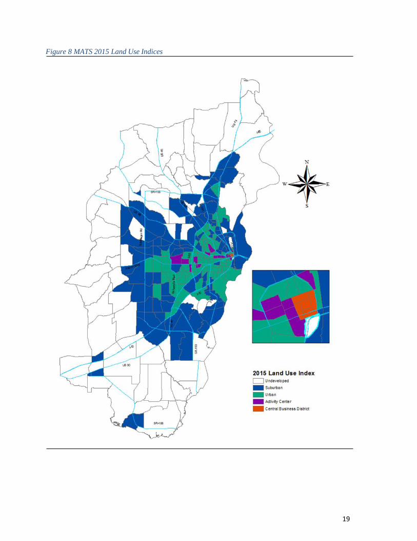
model chain. The result of this approach is shown on Figure 8 which illustrates 2015 conditions

and Figure 9 which shows 2045 indices. The break points (thresholds) were set at .5 units/acre

for suburban, 2.5/acre for urban, 10.0/acre for activity center, and 30.0 units/acre for CBD.

The true importance of the land use index is its use in determining network speeds and roadway

capacity. The speeds coded in the traffic models are often referred to as "free" speeds. They are not

the posted speeds or speed limits, but are intended to represent the actual average speed —

including intersection delay — of a vehicle during light traffic conditions. The coded speeds were

calculated from posted speeds using procedures found in the 1985 and 1994 Highway Capacity

Manuals and in NCHRP Report 387, Planning Techniques to Estimate Speeds and Service

Volumes for Planning Applications. Table 8 shows the assumed posted speeds by land use type

and roadway functional classification; it also includes the assumptions made regarding arterial

signal spacing. Table 9 summarizes the speeds coded in the MATS traffic models. The rela-

tively low speeds coded on freeways are to prevent them from attracting a disproportionate number

of trips and resulting in poor trip distribution and assignments in later stages of the model’s

application. The dominant pattern obvious from Tables 8 and 9 is an increase in speeds as

functional classification goes up, and an increase in speeds as development density goes down.

The "level-of-service" (LOS) concept is used to define the operational characteristics of roads at

various traffic volumes. It can be used to establish the most severe conditions which are accept-

able to the public. This is not to say or imply that the limits of acceptability are a desirable goal

— but simply that they are tolerable.

19

Figure 8 MATS 2015 Land Use Indices

20

Figure 9 MATS 2045 Land Use Indices

21

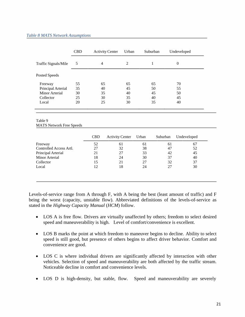
Table 8 MATS Network Assumptions

CBD Activity Center Urban Suburban Undeveloped

Traffic Signals/Mile

5

4

2

1

0

Posted Speeds

Freeway 55 65 65 65 70

Principal Arterial 35 40 45 50 55

Minor Arterial 30 35 40 45 50

Collector 25 30 35 40 45

Local 20 25 30 35 40

Table 9

MATS Network Free Speeds

CBD Activity Center Urban Suburban Undeveloped

Freeway 52 61 61 61 67 Controlled Access Artl. 27 32 38 47 52

Principal Arterial 21 27 33 42 45

Minor Arterial 18 24 30 37 40

Collector 15 21 27 32 37

Local 12 18 24 27 30

Levels-of-service range from A through F, with A being the best (least amount of traffic) and F

being the worst (capacity, unstable flow). Abbreviated definitions of the levels-of-service as

stated in the Highway Capacity Manual (HCM) follow.

• LOS A is free flow. Drivers are virtually unaffected by others; freedom to select desired

speed and maneuverability is high. Level of comfort/convenience is excellent.

• LOS B marks the point at which freedom to maneuver begins to decline. Ability to select

speed is still good, but presence of others begins to affect driver behavior. Comfort and

convenience are good.

• LOS C is where individual drivers are significantly affected by interaction with other

vehicles. Selection of speed and maneuverability are both affected by the traffic stream.

Noticeable decline in comfort and convenience levels.

• LOS D is high-density, but stable, flow. Speed and maneuverability are severely

22

restricted. Small traffic increases will cause operational problems. Comfort and

convenience levels are poor.

• LOS E is operation just below capacity. Speeds are reduced to low levels. Virtually no

room for maneuverability without forcing another vehicle to yield. Operation is usually

unstable, as any traffic increase causes breakdown. Comfort and convenience levels are

extremely poor; driver frustration is high.

• LOS F is forced, or breakdown, flow. Operation is characterized by stop-and-go waves

which are very unstable. The amount of traffic approaching a point is greater than the

amount which can pass the point.

For urban areas the size of Mobile, the minimum acceptable level-of-service is generally LOS D.

The conditions described above would usually occur only during a portion of the peak hour and

only on the most heavily traveled roads in the area. Based on accepted practices of traffic engi-

neering, the maximum flows (capacities) for LOS D for each type of road can be quantified. As

would be expected, the capacities of arterial and collector roads vary in inverse proportion to the

number of signals per mile and in direct proportion to the amount of available “green” time.

Therefore, land use and development densities play significant roles in determining capacity.

Conversely, uninterrupted flow (freeway) capacity is normally dependent only on posted speed.

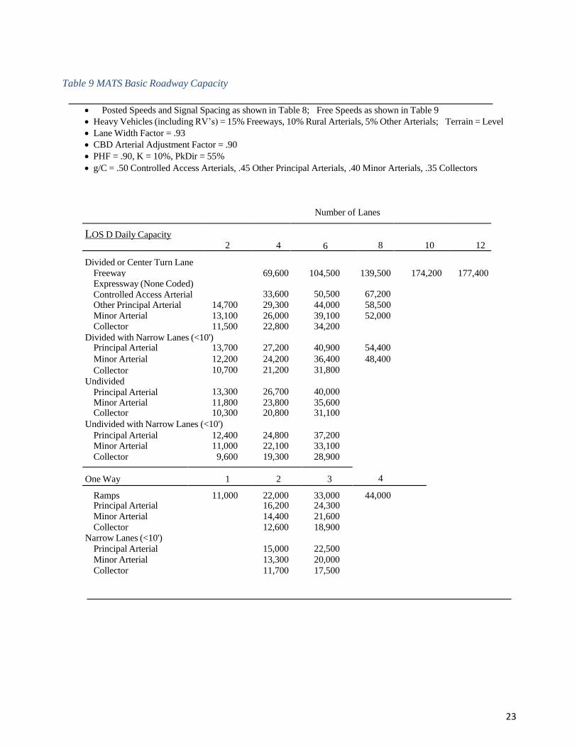
The capacity values ultimately used in the MATS models were derived from the procedures recom-

mended in TRB’s NCHRP Report 387. The assumptions used to calculate capacities and the basic

LOS D capacity values are contained in Table 10; a complete capacity table by link type as coded

with land use index and posted speed adjustments is given in Appendix A-6.

23

Table 9 MATS Basic Roadway Capacity

• Posted Speeds and Signal Spacing as shown in Table 8; Free Speeds as shown in Table 9

• Heavy Vehicles (including RV’s) = 15% Freeways, 10% Rural Arterials, 5% Other Arterials; Terrain = Level

• Lane Width Factor = .93

• CBD Arterial Adjustment Factor = .90

• PHF = .90, K = 10%, PkDir = 55%

• g/C = .50 Controlled Access Arterials, .45 Other Principal Arterials, .40 Minor Arterials, .35 Collectors

Number of Lanes

LOS D Daily Capacity

2 N

4

6

8

10

12

Divided or Center Turn Lane

Freeway

69,600

104,500

139,500

174,200

177,400

Expressway (None Coded)

Controlled Access Arterial

33,600

50,500

67,200

Other Principal Arterial 14,700 29,300 44,000 58,500 Minor Arterial 13,100 26,000 39,100 52,000 Collector 11,500 22,800 34,200

Divided with Narrow Lanes (<10') Principal Arterial 13,700 27,200 40,900 54,400

Minor Arterial 12,200 24,200 36,400 48,400

Collector

Undivided

Principal Arterial

10,700

13,300

21,200

26,700

31,800

40,000

Minor Arterial 11,800 23,800 35,600 Collector 10,300 20,800 31,100

Undivided with Narrow Lanes (<10')

Principal Arterial 12,400 24,800 37,200

4

Minor Arterial 11,000 22,100 33,100

Collector 9,600 19,300 28,900

One Way 1 2 3

Ramps 11,000 22,000 33,000 44,000 Principal Arterial 16,200 24,300 Minor Arterial 14,400 21,600 Collector 12,600 18,900

Narrow Lanes (<10') Principal Arterial 15,000 22,500 Minor Arterial 13,300 20,000 Collector 11,700 17,500

24

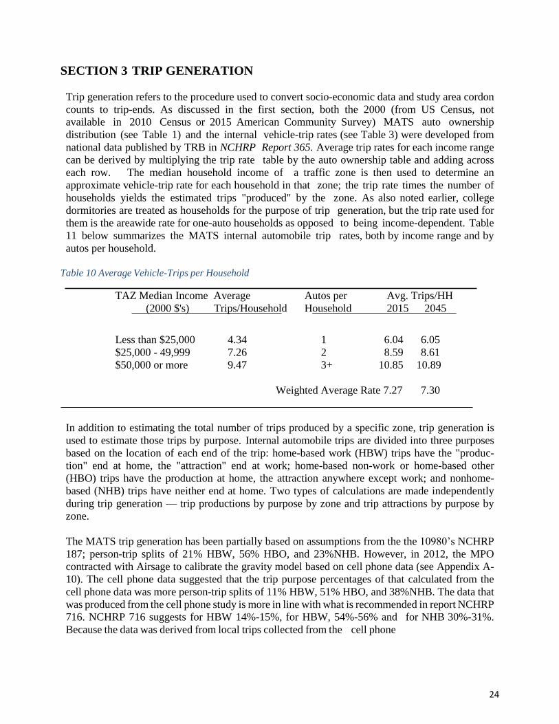
SECTION 3 TRIP GENERATION

Trip generation refers to the procedure used to convert socio-economic data and study area cordon

counts to trip-ends. As discussed in the first section, both the 2000 (from US Census, not

available in 2010 Census or 2015 American Community Survey) MATS auto ownership

distribution (see Table 1) and the internal vehicle-trip rates (see Table 3) were developed from

national data published by TRB in NCHRP Report 365. Average trip rates for each income range

can be derived by multiplying the trip rate table by the auto ownership table and adding across

each row. The median household income of a traffic zone is then used to determine an

approximate vehicle-trip rate for each household in that zone; the trip rate times the number of

households yields the estimated trips "produced" by the zone. As also noted earlier, college

dormitories are treated as households for the purpose of trip generation, but the trip rate used for

them is the areawide rate for one-auto households as opposed to being income-dependent. Table

11 below summarizes the MATS internal automobile trip rates, both by income range and by

autos per household.

Table 10 Average Vehicle-Trips per Household

TAZ Median Income Average Autos per Avg. Trips/HH

(2000 $'s) Trips/Household Household 2015 2045

Less than $25,000 4.34 1 6.04 6.05

$25,000 - 49,999 7.26 2 8.59 8.61

$50,000 or more 9.47 3+ 10.85 10.89

Weighted Average Rate 7.27 7.30

In addition to estimating the total number of trips produced by a specific zone, trip generation is

used to estimate those trips by purpose. Internal automobile trips are divided into three purposes

based on the location of each end of the trip: home-based work (HBW) trips have the "produc-

tion" end at home, the "attraction" end at work; home-based non-work or home-based other

(HBO) trips have the production at home, the attraction anywhere except work; and nonhome-

based (NHB) trips have neither end at home. Two types of calculations are made independently

during trip generation — trip productions by purpose by zone and trip attractions by purpose by

zone.

The MATS trip generation has been partially based on assumptions from the the 10980’s NCHRP

187; person-trip splits of 21% HBW, 56% HBO, and 23%NHB. However, in 2012, the MPO

contracted with Airsage to calibrate the gravity model based on cell phone data (see Appendix A-

10). The cell phone data suggested that the trip purpose percentages of that calculated from the

cell phone data was more person-trip splits of 11% HBW, 51% HBO, and 38%NHB. The data that

was produced from the cell phone study is more in line with what is recommended in report NCHRP

716. NCHRP 716 suggests for HBW 14%-15%, for HBW, 54%-56% and for NHB 30%-31%.

Because the data was derived from local trips collected from the cell phone

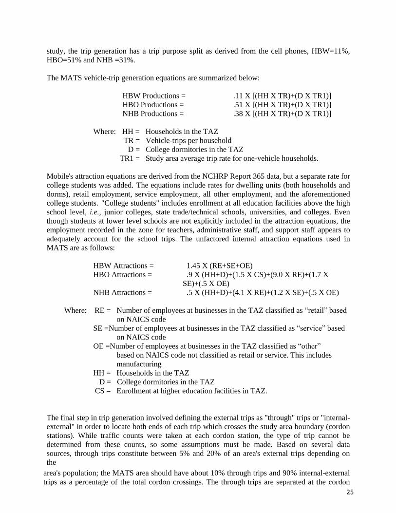
25

study, the trip generation has a trip purpose split as derived from the cell phones, HBW=11%,

HBO=51% and NHB =31%.

The MATS vehicle-trip generation equations are summarized below:

HBW Productions = .11 X [(HH X TR)+(D X TR1)]

HBO Productions = .51 X [(HH X TR)+(D X TR1)]

NHB Productions = .38 X [(HH X TR)+(D X TR1)]

Where: HH = Households in the TAZ

TR = Vehicle-trips per household

D = College dormitories in the TAZ

TR1 = Study area average trip rate for one-vehicle households.

Mobile's attraction equations are derived from the NCHRP Report 365 data, but a separate rate for

college students was added. The equations include rates for dwelling units (both households and

dorms), retail employment, service employment, all other employment, and the aforementioned

college students. "College students" includes enrollment at all education facilities above the high

school level, i.e., junior colleges, state trade/technical schools, universities, and colleges. Even

though students at lower level schools are not explicitly included in the attraction equations, the

employment recorded in the zone for teachers, administrative staff, and support staff appears to

adequately account for the school trips. The unfactored internal attraction equations used in

MATS are as follows:

HBW Attractions = 1.45 X (RE+SE+OE)

HBO Attractions = .9 X (HH+D)+(1.5 X CS)+(9.0 X RE)+(1.7 X

SE)+(.5 X OE)

NHB Attractions = .5 X (HH+D)+(4.1 X RE)+(1.2 X SE)+(.5 X OE)

Where: RE = Number of employees at businesses in the TAZ classified as “retail” based

on NAICS code

SE =Number of employees at businesses in the TAZ classified as “service” based

on NAICS code

OE =Number of employees at businesses in the TAZ classified as “other”

based on NAICS code not classified as retail or service. This includes

manufacturing

HH = Households in the TAZ

D = College dormitories in the TAZ

CS = Enrollment at higher education facilities in TAZ.

The final step in trip generation involved defining the external trips as "through" trips or "internal-

external" in order to locate both ends of each trip which crosses the study area boundary (cordon

stations). While traffic counts were taken at each cordon station, the type of trip cannot be

determined from these counts, so some assumptions must be made. Based on several data

sources, through trips constitute between 5% and 20% of an area's external trips depending on

the

area's population; the MATS area should have about 10% through trips and 90% internal-external

trips as a percentage of the total cordon crossings. The through trips are separated at the cordon

26

using a rate based on the functional classification of the facility; although logical, these rates are

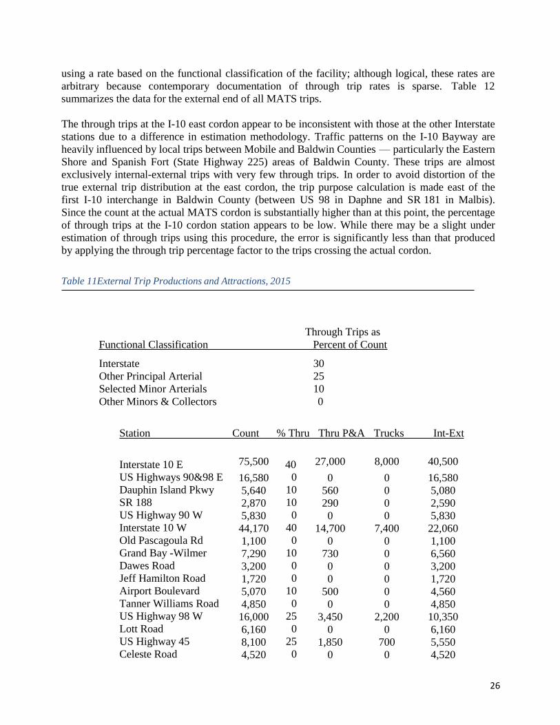
arbitrary because contemporary documentation of through trip rates is sparse. Table 12

summarizes the data for the external end of all MATS trips.

The through trips at the I-10 east cordon appear to be inconsistent with those at the other Interstate

stations due to a difference in estimation methodology. Traffic patterns on the I-10 Bayway are

heavily influenced by local trips between Mobile and Baldwin Counties — particularly the Eastern

Shore and Spanish Fort (State Highway 225) areas of Baldwin County. These trips are almost

exclusively internal-external trips with very few through trips. In order to avoid distortion of the

true external trip distribution at the east cordon, the trip purpose calculation is made east of the

first I-10 interchange in Baldwin County (between US 98 in Daphne and SR 181 in Malbis).

Since the count at the actual MATS cordon is substantially higher than at this point, the percentage

of through trips at the I-10 cordon station appears to be low. While there may be a slight under

estimation of through trips using this procedure, the error is significantly less than that produced

by applying the through trip percentage factor to the trips crossing the actual cordon.

Table 11External Trip Productions and Attractions, 2015

Through Trips as

Functional Classification Percent of Count

Interstate 30

Other Principal Arterial 25

Selected Minor Arterials 10

Other Minors & Collectors 0

Station Count % Thru Thru P&A Trucks Int-Ext

Interstate 10 E 75,500 40 27,000 8,000 40,500

US Highways 90&98 E 16,580 0 0 0 16,580 Dauphin Island Pkwy 5,640 10 560 0 5,080 SR 188 2,870 10 290 0 2,590 US Highway 90 W 5,830 0 0 0 5,830 Interstate 10 W 44,170 40 14,700 7,400 22,060 Old Pascagoula Rd 1,100 0 0 0 1,100 Grand Bay -Wilmer 7,290 10 730 0 6,560 Dawes Road 3,200 0 0 0 3,200 Jeff Hamilton Road 1,720 0 0 0 1,720 Airport Boulevard 5,070 10 500 0 4,560 Tanner Williams Road 4,850 0 0 0 4,850 US Highway 98 W 16,000 25 3,450 2,200 10,350 Lott Road 6,160 0 0 0 6,160 US Highway 45 8,100 25 1,850 700 5,550 Celeste Road 4,520 0 0 0 4,520

27

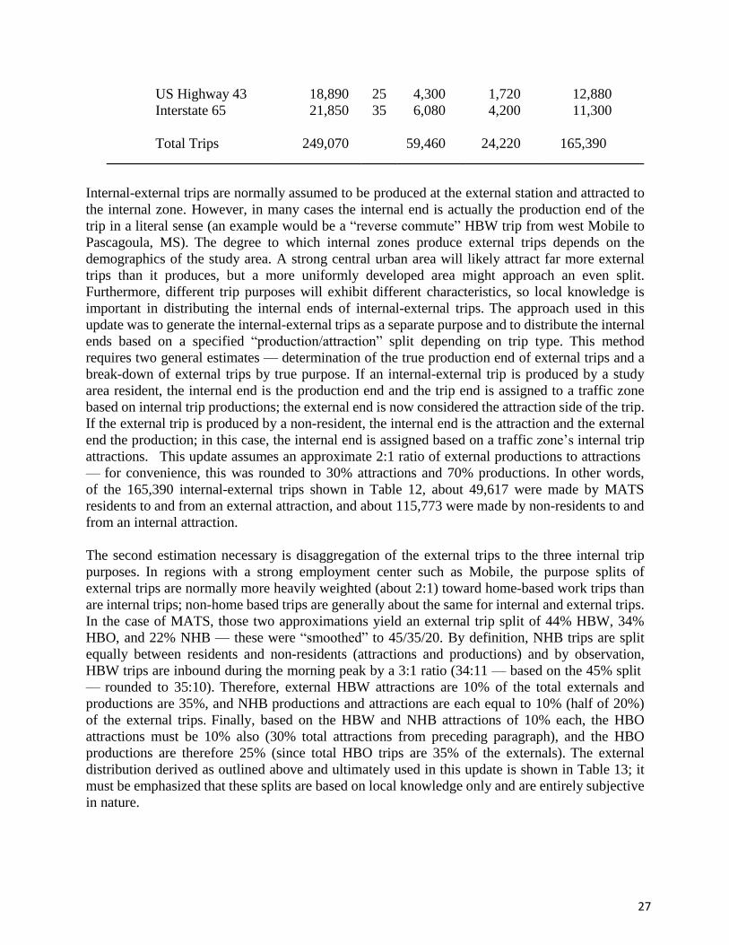
US Highway 43 18,890 25 4,300 1,720 12,880

Interstate 65 21,850 35 6,080 4,200 11,300

Total Trips 249,070

59,460 24,220 165,390

Internal-external trips are normally assumed to be produced at the external station and attracted to

the internal zone. However, in many cases the internal end is actually the production end of the

trip in a literal sense (an example would be a “reverse commute” HBW trip from west Mobile to

Pascagoula, MS). The degree to which internal zones produce external trips depends on the

demographics of the study area. A strong central urban area will likely attract far more external

trips than it produces, but a more uniformly developed area might approach an even split.

Furthermore, different trip purposes will exhibit different characteristics, so local knowledge is

important in distributing the internal ends of internal-external trips. The approach used in this

update was to generate the internal-external trips as a separate purpose and to distribute the internal

ends based on a specified “production/attraction” split depending on trip type. This method

requires two general estimates — determination of the true production end of external trips and a

break-down of external trips by true purpose. If an internal-external trip is produced by a study

area resident, the internal end is the production end and the trip end is assigned to a traffic zone

based on internal trip productions; the external end is now considered the attraction side of the trip.

If the external trip is produced by a non-resident, the internal end is the attraction and the external

end the production; in this case, the internal end is assigned based on a traffic zone’s internal trip

attractions. This update assumes an approximate 2:1 ratio of external productions to attractions

— for convenience, this was rounded to 30% attractions and 70% productions. In other words,

of the 165,390 internal-external trips shown in Table 12, about 49,617 were made by MATS

residents to and from an external attraction, and about 115,773 were made by non-residents to and

from an internal attraction.

The second estimation necessary is disaggregation of the external trips to the three internal trip

purposes. In regions with a strong employment center such as Mobile, the purpose splits of

external trips are normally more heavily weighted (about 2:1) toward home-based work trips than

are internal trips; non-home based trips are generally about the same for internal and external trips.

In the case of MATS, those two approximations yield an external trip split of 44% HBW, 34%

HBO, and 22% NHB — these were “smoothed” to 45/35/20. By definition, NHB trips are split

equally between residents and non-residents (attractions and productions) and by observation,

HBW trips are inbound during the morning peak by a 3:1 ratio (34:11 — based on the 45% split

— rounded to 35:10). Therefore, external HBW attractions are 10% of the total externals and

productions are 35%, and NHB productions and attractions are each equal to 10% (half of 20%)

of the external trips. Finally, based on the HBW and NHB attractions of 10% each, the HBO

attractions must be 10% also (30% total attractions from preceding paragraph), and the HBO

productions are therefore 25% (since total HBO trips are 35% of the externals). The external

distribution derived as outlined above and ultimately used in this update is shown in Table 13; it

must be emphasized that these splits are based on local knowledge only and are entirely subjective

in nature.

28

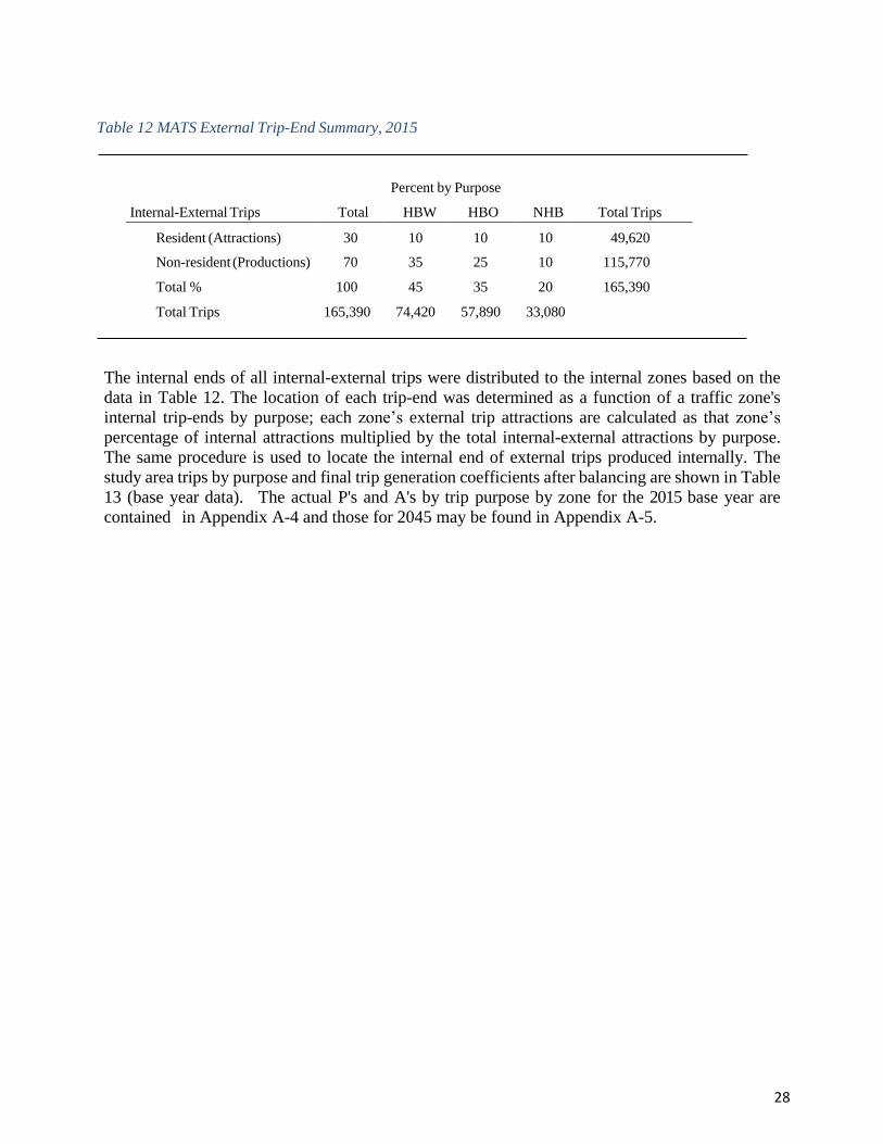
Table 12 MATS External Trip-End Summary, 2015

Percent by Purpose

Internal-External Trips Total HBW HBO NHB Total Trips

Resident (Attractions) 30 10 10 10 49,620

Non-resident (Productions) 70 35 25 10 115,770

Total % 100 45 35 20 165,390

Total Trips 165,390 74,420 57,890 33,080

The internal ends of all internal-external trips were distributed to the internal zones based on the

data in Table 12. The location of each trip-end was determined as a function of a traffic zone's

internal trip-ends by purpose; each zone’s external trip attractions are calculated as that zone’s

percentage of internal attractions multiplied by the total internal-external attractions by purpose.

The same procedure is used to locate the internal end of external trips produced internally. The

study area trips by purpose and final trip generation coefficients after balancing are shown in Table

13 (base year data). The actual P's and A's by trip purpose by zone for the 2015 base year are

contained in Appendix A-4 and those for 2045 may be found in Appendix A-5.

29

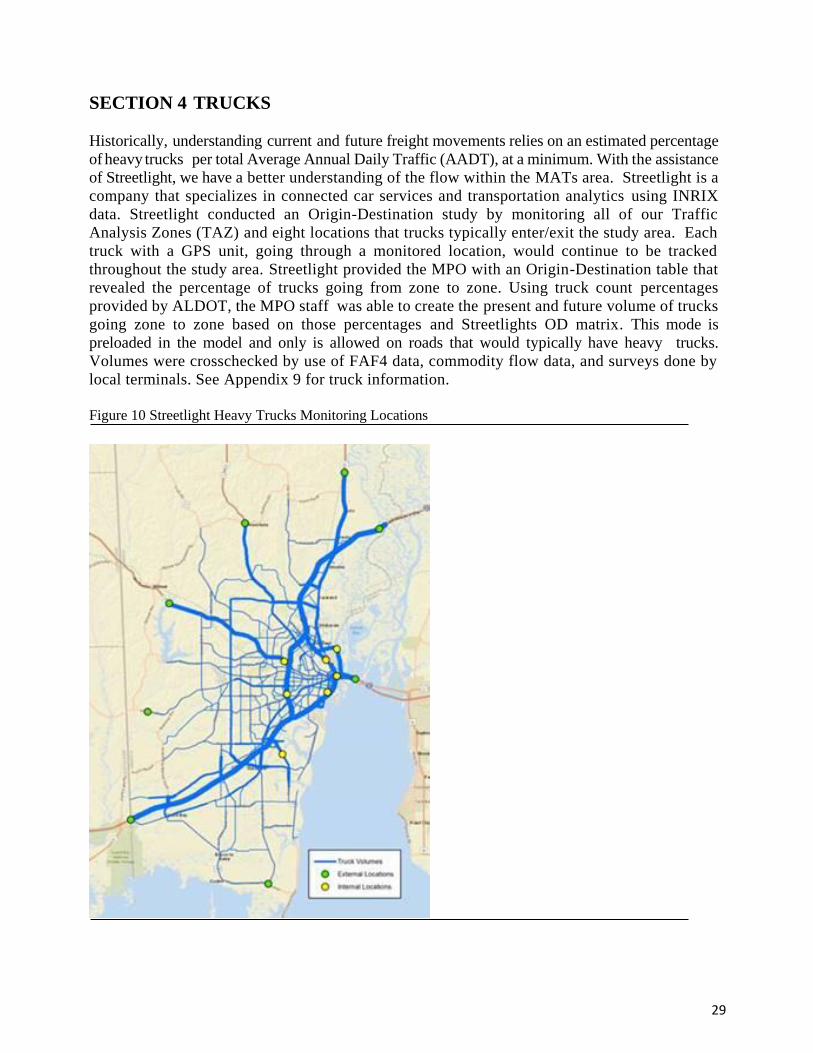
SECTION 4 TRUCKS

Historically, understanding current and future freight movements relies on an estimated percentage

of heavy trucks per total Average Annual Daily Traffic (AADT), at a minimum. With the assistance

of Streetlight, we have a better understanding of the flow within the MATs area. Streetlight is a

company that specializes in connected car services and transportation analytics using INRIX

data. Streetlight conducted an Origin-Destination study by monitoring all of our Traffic

Analysis Zones (TAZ) and eight locations that trucks typically enter/exit the study area. Each

truck with a GPS unit, going through a monitored location, would continue to be tracked

throughout the study area. Streetlight provided the MPO with an Origin-Destination table that

revealed the percentage of trucks going from zone to zone. Using truck count percentages

provided by ALDOT, the MPO staff was able to create the present and future volume of trucks

going zone to zone based on those percentages and Streetlights OD matrix. This mode is

preloaded in the model and only is allowed on roads that would typically have heavy trucks.

Volumes were crosschecked by use of FAF4 data, commodity flow data, and surveys done by

local terminals. See Appendix 9 for truck information.

Figure 10 Streetlight Heavy Trucks Monitoring Locations

30

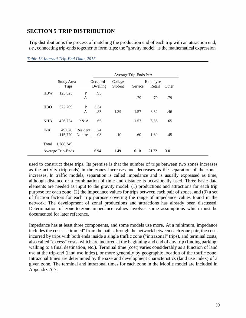
SECTION 5 TRIP DISTRIBUTION

Trip distribution is the process of matching the production end of each trip with an attraction end,

i.e., connecting trip-ends together to form trips; the "gravity model" is the mathematical expression

Table 13 Internal Trip-End Data, 2015

Average Trip-Ends Per:

Study Area Occupied College Employee

Trips Dwelling Student Service Retail Other

HBW 123,525 P

A

.95 .79

.79

.79

HBO 572,709 P 3.34

A .83 1.39 1.57 8.32 .46

NHB 426,724 P & A .65 1.57 5.36 .65

INX 49,620 Resident .24

115,770 Non-res. .08 .10 .60 1.39 .45

Total 1,288,345

Average Trip-Ends 6.94 1.49 6.10 21.22 3.01

used to construct these trips. Its premise is that the number of trips between two zones increases

as the activity (trip-ends) in the zones increases and decreases as the separation of the zones

increases. In traffic models, separation is called impedance and is usually expressed as time,

although distance or a combination of time and distance is occasionally used. Three basic data

elements are needed as input to the gravity model: (1) productions and attractions for each trip

purpose for each zone, (2) the impedance values for trips between each pair of zones, and (3) a set

of friction factors for each trip purpose covering the range of impedance values found in the

network. The development of zonal productions and attractions has already been discussed.

Determination of zone-to-zone impedance values involves some assumptions which must be

documented for later reference.

Impedance has at least three components, and some models use more. At a minimum, impedance

includes the costs "skimmed" from the paths through the network between each zone pair, the costs

incurred by trips with both ends inside a single traffic zone ("intrazonal" trips), and terminal costs,

also called "excess" costs, which are incurred at the beginning and end of any trip (finding parking,

walking to a final destination, etc.). Terminal time (cost) varies considerably as a function of land

use at the trip-end (land use index), or more generally by geographic location of the traffic zone.

Intrazonal times are determined by the size and development characteristics (land use index) of a

given zone. The terminal and intrazonal times for each zone in the Mobile model are included in

Appendix A-7.

31

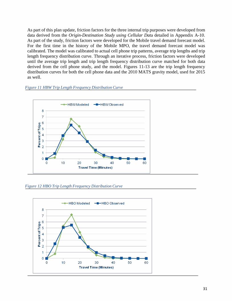
As part of this plan update, friction factors for the three internal trip purposes were developed from

data derived from the Origin-Destination Study using Cellular Data detailed in Appendix A-10.

As part of the study, friction factors were developed for the Mobile travel demand forecast model.

For the first time in the history of the Mobile MPO, the travel demand forecast model was

calibrated. The model was calibrated to actual cell phone trip patterns, average trip lengths and trip

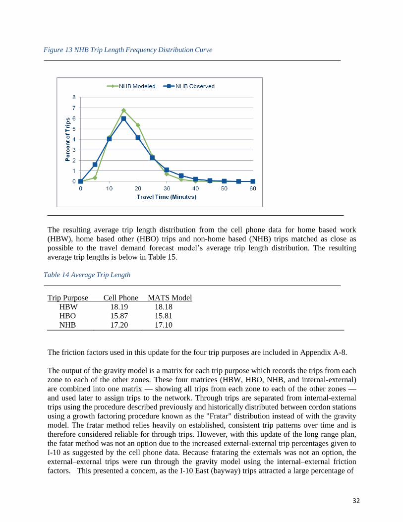
length frequency distribution curve. Through an iterative process, friction factors were developed

until the average trip length and trip length frequency distribution curve matched for both data

derived from the cell phone study, and the model. Figures 11-13 are the trip length frequency

distribution curves for both the cell phone data and the 2010 MATS gravity model, used for 2015

as well.

Figure 11 HBW Trip Length Frequency Distribution Curve

Figure 12 HBO Trip Length Frequency Distribution Curve

32

Figure 13 NHB Trip Length Frequency Distribution Curve

The resulting average trip length distribution from the cell phone data for home based work

(HBW), home based other (HBO) trips and non-home based (NHB) trips matched as close as

possible to the travel demand forecast model’s average trip length distribution. The resulting

average trip lengths is below in Table 15.

Table 14 Average Trip Length

Trip Purpose Cell Phone MATS Model

HBW 18.19 18.18 HBO 15.87 15.81

NHB 17.20 17.10

The friction factors used in this update for the four trip purposes are included in Appendix A-8.

The output of the gravity model is a matrix for each trip purpose which records the trips from each

zone to each of the other zones. These four matrices (HBW, HBO, NHB, and internal-external)

are combined into one matrix — showing all trips from each zone to each of the other zones —

and used later to assign trips to the network. Through trips are separated from internal-external

trips using the procedure described previously and historically distributed between cordon stations

using a growth factoring procedure known as the "Fratar" distribution instead of with the gravity

model. The fratar method relies heavily on established, consistent trip patterns over time and is

therefore considered reliable for through trips. However, with this update of the long range plan,

the fatar method was not an option due to the increased external-external trip percentages given to

I-10 as suggested by the cell phone data. Because frataring the externals was not an option, the

external–external trips were run through the gravity model using the internal–external friction

factors. This presented a concern, as the I-10 East (bayway) trips attracted a large percentage of

33

trips coming from I-65 North overloading I-165 with external-external trips. Knowing that any trip

coming south on I-65 to Baldwin County, would have already exited from I-65 in Baldwin County

on either US 59 or SR 225. For this reason K-factors were used for that external zone pair only (I-

65 to I-10 East). K-factors allow the trips between the zonal pairs to be modified to realistic

patterns.

It should be noted that the MATS models do not allow several physically possible through

movements which are illogical due to 180 paths or preferable routes outside the study area.

Appendix 6 lists the external zones which have through movements and the pairs which are

permitted.

5.1 Preloading

The MATS traffic model "preloads" trucks and through trips on the network prior to the

assignment of internal trips. Trucks are assigned to only the roads that heavy trucks would travel,

and only to and from externals and Freight Analysis Zones (FAZs). The TAZ to FAZ equivalency

table is in Appendix A9. Similarly, the through trips are not necessarily assigned to the quickest

path between a pair of zones, but to a route that has been determined to be the most probable for a

trip traversing the entire study area (generally only federal and some state highways). The

purpose of this approach is two-fold — to keep the through trips on higher level "posted" facilities

and to prevent diversion of through traffic during capacity-restrained assignments.

The preloading is accomplished by coding the assignment group in the link record file 1 through

4. An assignment code “1" means the link is on a route determined to allow vehicles and trucks,

but no vehicle preloads. Links with assignment group code 2, allow vehicle trips and vehicle

through trips. There are no links with an assignment group code 3 (which means all trips are

allowed) and links with assignment group code 4 are not allowed to have trucks or preloaded

vehicles, only internal and internal external trips. An external-external trip table is added to the

origin-destination table that the network is assigned to. Trucks are considered mode 2 and the

preloads are considered as a third mode (mode 3) in the model and are merely assigned (all-or-

nothing) to the network to only those links that have and assignment group code of “2". Figure

14 is a schematic plot of the 2015 network showing preloaded through trips for vehicles and Figure

15 shows preloaded truck trips.

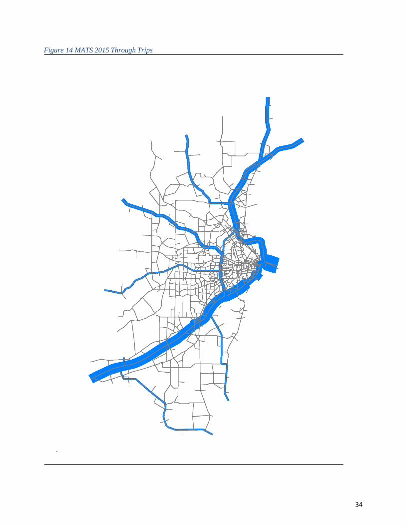
34

Figure 14 MATS 2015 Through Trips

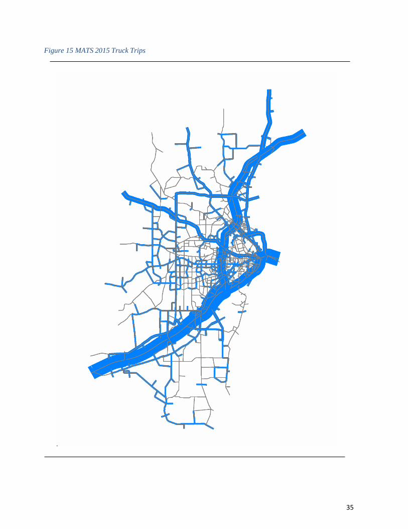
35

Figure 15 MATS 2015 Truck Trips

36

SECTION 6 TRAFFIC ASSINGMENT AND MODEL VALIDATION

Traffic assignment is basically the product of the entire modeling procedure; all prior steps in

developing the model are brought together at this point. Traffic assignment refers to placing the

trip matrix (the trips from each zone to each other zone) on the individual facilities which make

up the highway network. Models use one of three types of assignment: all-or-nothing, capacity

restraint, or random. All-or-nothing assigns all trips between each zone pair to the minimum time

path (quickest route), regardless of the total number of trips assigned to those roads relative to their

capacity limitations. Capacity restraint is an iterative assignment procedure which adjusts paths

between each network loading to account for lower speeds due to congestion on the minimum time

path between each zone pair; thus, different paths may be selected during different iterations. -

Two basic options are available for capacity restraint assignments (depending on software) — the

user controls the total number and weighting of each iteration to determine the final assignment,

or the iterations continue at weightings which are based on "optimum" or balanced conditions as

determined by the software (equilibrium assignment). Random (stochastic or multi-route)

assignment is based on the premise that more than one desirable path exists between each zone

pair; the desirability of each path can be calculated with several methods and certain capacity

restraint procedures can be effectively used. The distinction between stochastic models and

capacity restraint all-or-nothing models fades depending on the type of capacity restraint used.

The traffic assignment methodology used in this update was equilibrium assignment with user-

specified convergence and speed-capacity (volume-delay) curves.

Many of the adjustments and refinements mentioned in previous portions of this section cannot

actually be made until after at least one assignment is completed, allowing a rough estimate of the

trip movements and traffic patterns produced by the model and its empirical assumptions. The

process of comparing a model's estimate of traffic to the traffic counts actually taken in the field

is called "validation". Validation allows the error of the model to be minimized and its confidence

limits to be established. Validation includes verification of network and facility assumptions,

checks on areawide trip movement, and ultimately, the accuracy of assignments on individual

links. Thus, validation is an iterative process of model development whereby the entire model

chain is repeated numerous times as individual model parameters are modified and the assignment

results compared — to each other as well as to actual conditions. Due to the nature of this

document, great detail is not provided on the specifics of validation, but rather the process and

results. Preceding portions of this report have detailed the end result of each stage of model

development after completion of validation (i.e., after inaccuracies were discovered and

corrected). Similarly, this section provides comparisons between the final model assignments,

ground counts, and acceptable error limits and outlines the end-product without delving into the

numerous and varied paths taken to get there.

6.1 Traffic Counts

The Alabama Department of Transportation (ALDOT) took traffic counts throughout the study

area in 2015. However, because half of the traffic counts were taken before

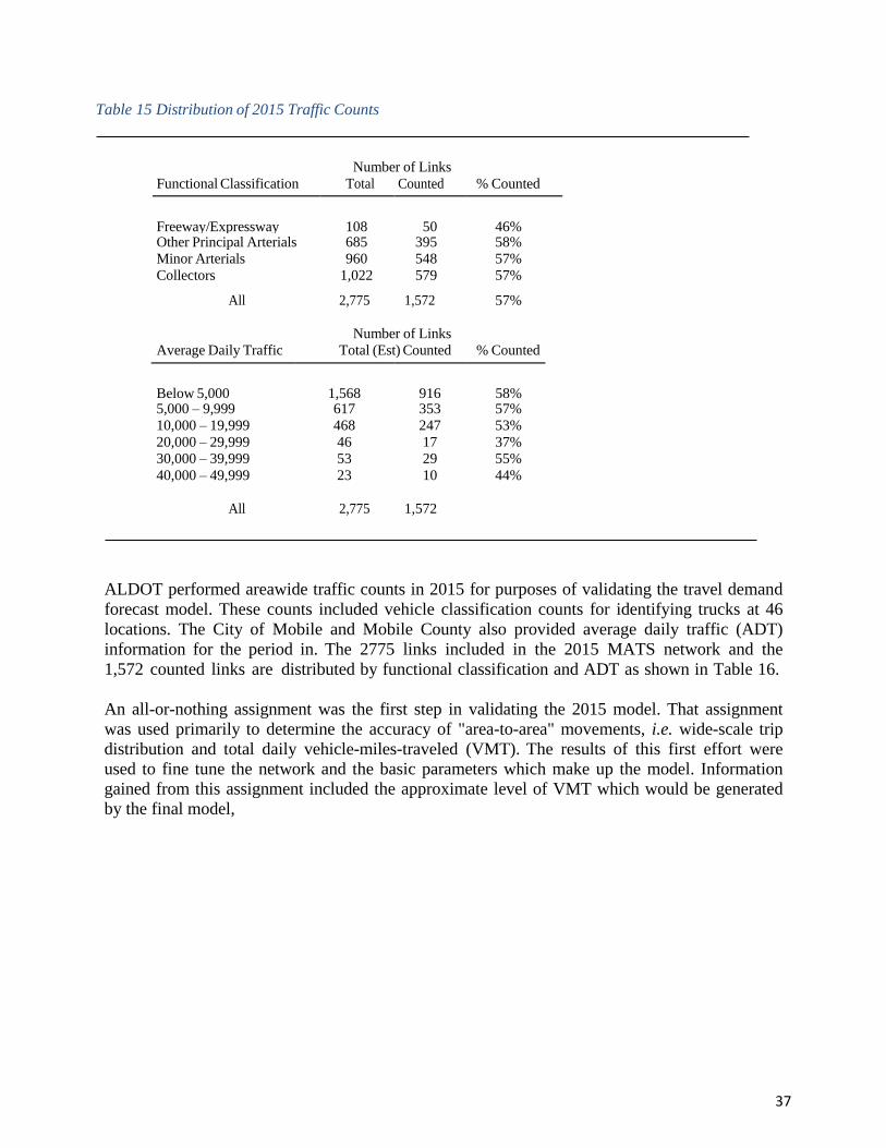
37

Table 15 Distribution of 2015 Traffic Counts

Number of Links

Functional Classification Total Counted % Counted

Freeway/Expressway

108

50

46%

Other Principal Arterials 685 395 58%

Minor Arterials 960 548 57%

Collectors 1,022 579 57%

All 2,775 1,572 57%

Number of Links

Average Daily Traffic Total (Est) Counted % Counted

Below 5,000

1,568

916

58%

5,000 – 9,999 617 353

57%

10,000 – 19,999 468 247 53%

20,000 – 29,999 46 17 37%

30,000 – 39,999 53 29 55%

40,000 – 49,999 23 10 44%

All 2,775 1,572

ALDOT performed areawide traffic counts in 2015 for purposes of validating the travel demand

forecast model. These counts included vehicle classification counts for identifying trucks at 46

locations. The City of Mobile and Mobile County also provided average daily traffic (ADT)

information for the period in. The 2775 links included in the 2015 MATS network and the

1,572 counted links are distributed by functional classification and ADT as shown in Table 16.

An all-or-nothing assignment was the first step in validating the 2015 model. That assignment

was used primarily to determine the accuracy of "area-to-area" movements, i.e. wide-scale trip

distribution and total daily vehicle-miles-traveled (VMT). The results of this first effort were

used to fine tune the network and the basic parameters which make up the model. Information

gained from this assignment included the approximate level of VMT which would be generated

by the final model,

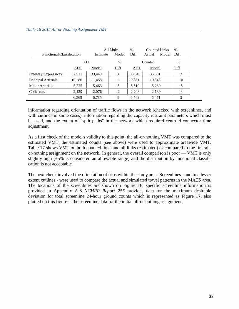
38

Table 16 2015 All-or-Nothing Assignment VMT

Functional Classification

ALL % Counted %

information regarding orientation of traffic flows in the network (checked with screenlines, and

with cutlines in some cases), information regarding the capacity restraint parameters which must

be used, and the extent of "split paths" in the network which required centroid connector time

adjustment.

As a first check of the model's validity to this point, the all-or-nothing VMT was compared to the

estimated VMT; the estimated counts (see above) were used to approximate areawide VMT.

Table 17 shows VMT on both counted links and all links (estimated) as compared to the first all-

or-nothing assignment on the network. In general, the overall comparison is poor — VMT is only

slightly high (±5% is considered an allowable range) and the distribution by functional classifi-

cation is not acceptable.

The next check involved the orientation of trips within the study area. Screenlines - and to a lesser

extent cutlines - were used to compare the actual and simulated travel patterns in the MATS area.

The locations of the screenlines are shown on Figure 16; specific screenline information is

provided in Appendix A-8. NCHRP Report 255 provides data for the maximum desirable

deviation for total screenline 24-hour ground counts which is represented as Figure 17; also

plotted on this figure is the screenline data for the initial all-or-nothing assignment.

All Links

%

Counted Links

%

Estimate Model Diff Actual Model Diff

ADT Model Diff ADT Model Diff

Freeway/Expressway 32,511 33,449 3 33,043 35,601 7

Principal Arterials 10,286 11,458 11 9,861 10,843 10

Minor Arterials 5,725 5,463 -5 5,519 5,239 -5

Collectors 2,129 2,076 -2 2,208 2,139 -3

6,569 6,785 3 6,569 6,471 3

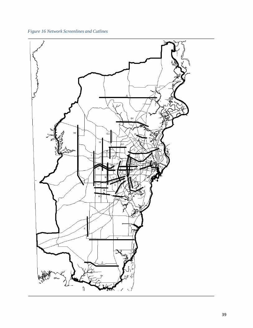
39

Figure 16 Network Screenlines and Cutlines

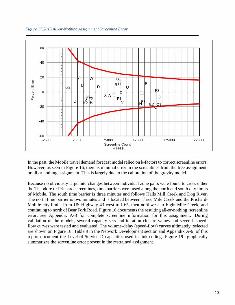
40

Figure 17 2015 All-or-Nothing Assig nment Screenline Error

In the past, the Mobile travel demand forecast model relied on k-factors to correct screenline errors.

However, as seen in Figure 16, there is minimal error in the screenlines from the free assignment,

or all or nothing assignment. This is largely due to the calibration of the gravity model.

Because no obviously large interchanges between individual zone pairs were found to cross either

the Theodore or Prichard screenlines, time barriers were used along the north and south city limits

of Mobile. The south time barrier is three minutes and follows Halls Mill Creek and Dog River.

The north time barrier is two minutes and is located between Three Mile Creek and the Prichard-

Mobile city limits from US Highway 43 west to I-65, then northwest to Eight Mile Creek, and

continuing to north of Bear Fork Road. Figure 16 documents the resulting all-or-nothing screenline

error; see Appendix A-8 for complete screenline information for this assignment. During

validation of the models, several capacity sets and iteration closure values and several speed-

flow curves were tested and evaluated. The volume-delay (speed-flow) curves ultimately selected

are shown on Figure 18; Table 9 in the Network Development section and Appendix A-6 of this

report document the Level-of-Service D capacities used in link coding. Figure 19 graphically

summarizes the screenline error present in the restrained assignment.

A

B1

B

CC1

D

E1

E2

F1F2

F3

G1

G2H

IJ

K1K2

L

M

N

O

P

Q

RST

U

V

W

X

Y

Z

-60

-40

-20

0

20

40

60

-25000 25000 75000 125000 175000 225000

Perc

ent

Err

or

Screenline CountFree

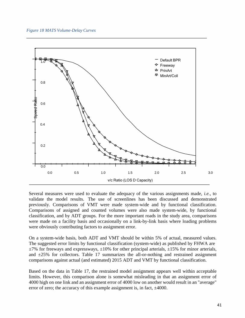
41

Figure 18 MATS Volume-Delay Curves

1.0

0.8

0.6

0.4

0.2

0.0

0.0 0.5 1.0 1.5 2.0 2.5 3.0

v/c Ratio (LOS D Capacity)

Several measures were used to evaluate the adequacy of the various assignments made, i.e., to

validate the model results. The use of screenlines has been discussed and demonstrated

previously. Comparisons of VMT were made system-wide and by functional classification.

Comparisons of assigned and counted volumes were also made system-wide, by functional

classification, and by ADT groups. For the more important roads in the study area, comparisons

were made on a facility basis and occasionally on a link-by-link basis where loading problems

were obviously contributing factors to assignment error.

On a system-wide basis, both ADT and VMT should be within 5% of actual, measured values.

The suggested error limits by functional classification (system-wide) as published by FHWA are

±7% for freeways and expressways, ±10% for other principal arterials, ±15% for minor arterials,

and ±25% for collectors. Table 17 summarizes the all-or-nothing and restrained assignment

comparisons against actual (and estimated) 2015 ADT and VMT by functional classification.

Based on the data in Table 17, the restrained model assignment appears well within acceptable

limits. However, this comparison alone is somewhat misleading in that an assignment error of

4000 high on one link and an assignment error of 4000 low on another would result in an "average"

error of zero; the accuracy of this example assignment is, in fact, ±4000.

Default BPR

Freeway

PrinArt

Sp

ee

d R

atio

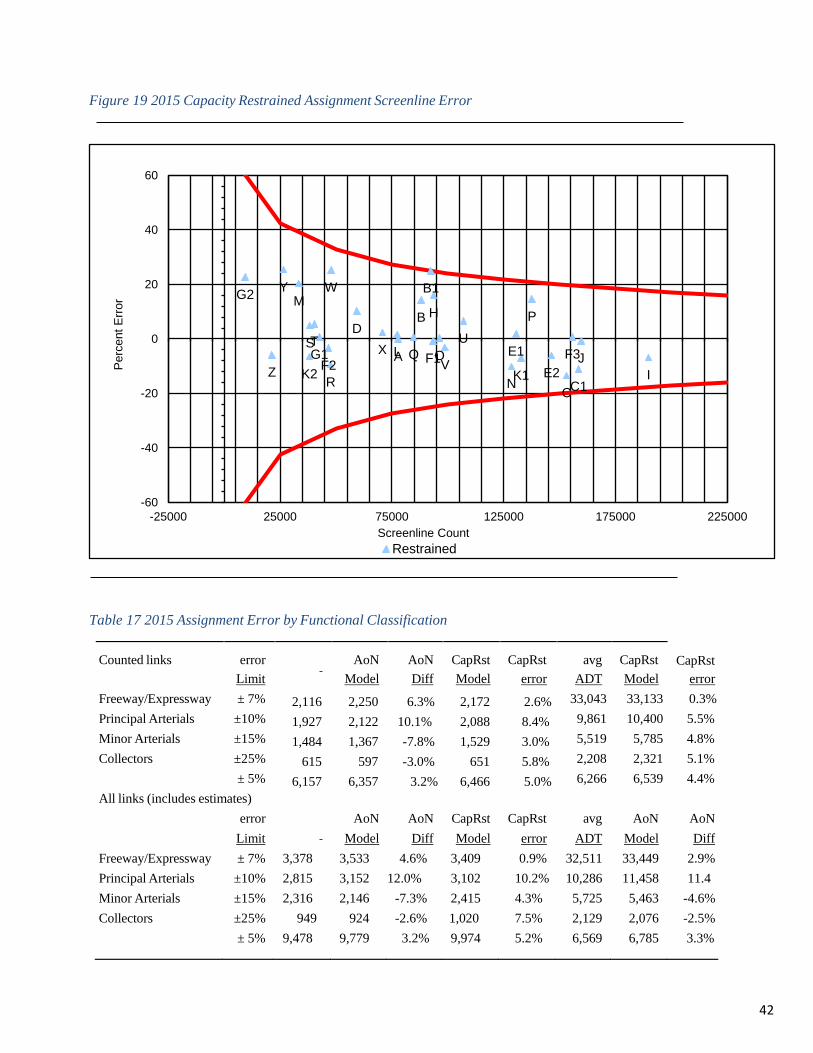
42

Figure 19 2015 Capacity Restrained Assignment Screenline Error

Table 17 2015 Assignment Error by Functional Classification

Counted links error

AoN AoN CapRst CapRst avg CapRst CapRst

Limit Model Diff Model error ADT Model error

Freeway/Expressway ± 7% 2,116 2,250 6.3% 2,172 2.6% 33,043 33,133 0.3%

Principal Arterials ±10% 1,927 2,122 10.1% 2,088 8.4% 9,861 10,400 5.5%

Minor Arterials ±15% 1,484 1,367 -7.8% 1,529 3.0% 5,519 5,785 4.8%

Collectors ±25% 615 597 -3.0% 651 5.8% 2,208 2,321 5.1%

± 5% 6,157 6,357 3.2% 6,466 5.0% 6,266 6,539 4.4%

All links (includes estimates)

error AoN AoN CapRst CapRst avg AoN AoN

Limit Model Diff Model error ADT Model Diff

Freeway/Expressway ± 7% 3,378

3,533 4.6% 3,409 0.9% 32,511 33,449 2.9%

Principal Arterials ±10% 2,815 3,152 12.0% 3,102 10.2% 10,286 11,458 11.4

Minor Arterials ±15% 2,316 2,146 -7.3% 2,415 4.3% 5,725 5,463 -4.6%

Collectors ±25% 949 924 -2.6% 1,020 7.5% 2,129 2,076 -2.5%

± 5% 9,478 9,779 3.2% 9,974 5.2% 6,569 6,785 3.3%

A

B1

B

CC1

D

E1

E2F1

F2F3G1

G2

H

I

J

K1K2

L

M

N

O

P

Q

R

ST U

V

W

X

Y

Z

-60

-40

-20

0

20

40

60

-25000 25000 75000 125000 175000 225000

Perc

ent

Err

or

Screenline Count

Restrained

43

A much more meaningful measure of model accuracy is the concept of "Root-Mean-Square", or

RMS, error. In general terms, RMS error is roughly equal to the average of the absolute values

of the individual errors; thus, the RMS error of the above example would be about 4000 instead of

0. To illustrate the substantial differences of the two error measurement standards, Table 19

below compares the 2015 assignment RMS error to the average error as given in Table 18.

Table 18 Comparison of Average and RMS Error by Functional Classification

Avg AoN RMS CpRst RMS

Functional Classification ADT Model Error Error Model Error Error

(Counted Links Only)

Freeway/Expressway 33,043 35,601 7.7% 14.3% 33,133 0.3%

11.0% Other Principal Arterials 9,861 10,843 10.0% 29.0% 10,400 5.5% 24.2%

Minor Arterials 5,519 5,239 -5.1% 37.8% 5,785 4.8% 39.3%

Collectors 2,208 2,139 -3.1% 74.2% 2,321 5.1% 75.3%

Total 6,266 6,471 3.3% 36.6% 6,539 4.4% 33.9%

(All Links - includes estimates)

Freeway/Expressway 32,511 33,449 2.9% 14.8% 31,566 -2.9% 12.9% Other Principal Arterials 10,286 11,458 11.4

% 31.7% 10,977 6.7% 26.8%

Minor Arterials 5,725 5,463 -4.6% 37.8% 6,010 5.0% 38.8%

Collectors 2,129 2,076 -2.5% 88.8% 2,260 6.1% 89.9%

Total 6,569 6,785 3.3% 35.9% 6,850 4.3% 33.8%

Since some error is expected in the traffic counts to which the assignment is compared, and since

some error will be present in any model simulation no matter how good, the concept of allowable

RMS error is used in analyzing assignment accuracy similar to the way maximum allowable

screenline error was used in evaluating general travel patterns — the higher the volume, the lower

the allowable percentage error. Since every link in the network will probably not be within the

established error limits, links are usually grouped based on the counted (or estimated) ADT. The

RMS error of each of these ranges is then compared to the error limitations to evaluate the overall

performance of the model. Table 20 includes the maximum allowable percentage error based on

ADT range and summarizes the 2015 assignments in relation to these standards; the data in Table

20 is also shown graphically on Figure 20. As is obvious from Table 20 and Figure 20, the

capacity restrained model assignment is well within the established error limits for grouped ADT

data.

As a final and most stringent comparison, link-by-link scatter plots of the all-or-nothing and

capacity restrained assignments were constructed. The resulting plots are shown in Figures 21.

Figure 21 includes plots of both assignments and is based on the model's actual error for each link.

The lines above and below the diagonal axis indicate the desired maximum and minimum error

ranges. This type of plot shows any bias of the model in terms of under or over-assignment in

any given ADT range. It is best used for major corrections early in the model development

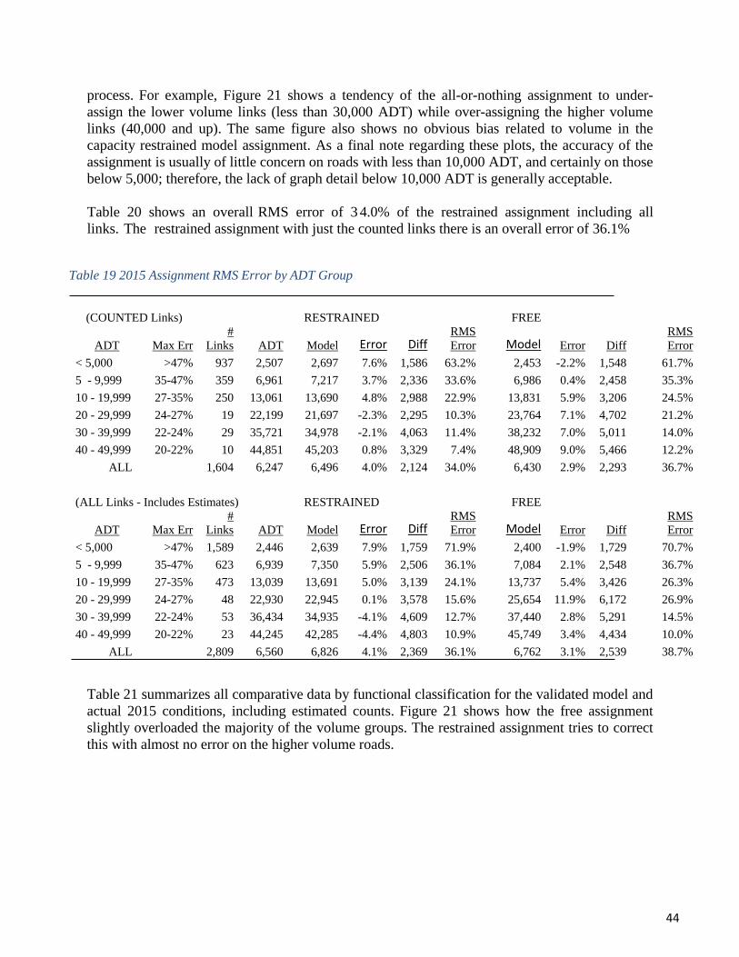
44

process. For example, Figure 21 shows a tendency of the all-or-nothing assignment to under-

assign the lower volume links (less than 30,000 ADT) while over-assigning the higher volume

links (40,000 and up). The same figure also shows no obvious bias related to volume in the

capacity restrained model assignment. As a final note regarding these plots, the accuracy of the

assignment is usually of little concern on roads with less than 10,000 ADT, and certainly on those

below 5,000; therefore, the lack of graph detail below 10,000 ADT is generally acceptable.

Table 20 shows an overall RMS error of 3 4.0% of the restrained assignment including all

links. The restrained assignment with just the counted links there is an overall error of 36.1%

Table 19 2015 Assignment RMS Error by ADT Group

(COUNTED Links) RESTRAINED FREE

ADT Max Err

#

Links ADT Model Error Diff RMS

Error Model Error Diff

RMS

Error

< 5,000 >47% 937 2,507 2,697 7.6% 1,586 63.2% 2,453 -2.2% 1,548 61.7%

5 - 9,999 35-47% 359 6,961 7,217 3.7% 2,336 33.6% 6,986 0.4% 2,458 35.3%

10 - 19,999 27-35% 250 13,061 13,690 4.8% 2,988 22.9% 13,831 5.9% 3,206 24.5%

20 - 29,999 24-27% 19 22,199 21,697 -2.3% 2,295 10.3% 23,764 7.1% 4,702 21.2%

30 - 39,999 22-24% 29 35,721 34,978 -2.1% 4,063 11.4% 38,232 7.0% 5,011 14.0%

40 - 49,999 20-22% 10 44,851 45,203 0.8% 3,329 7.4% 48,909 9.0% 5,466 12.2%

ALL 1,604 6,247 6,496 4.0% 2,124 34.0% 6,430 2.9% 2,293 36.7%

(ALL Links - Includes Estimates) RESTRAINED FREE

ADT Max Err

#

Links ADT Model Error Diff RMS

Error Model Error Diff

RMS

Error

< 5,000 >47% 1,589 2,446 2,639 7.9% 1,759 71.9% 2,400 -1.9% 1,729 70.7%

5 - 9,999 35-47% 623 6,939 7,350 5.9% 2,506 36.1% 7,084 2.1% 2,548 36.7%

10 - 19,999 27-35% 473 13,039 13,691 5.0% 3,139 24.1% 13,737 5.4% 3,426 26.3%

20 - 29,999 24-27% 48 22,930 22,945 0.1% 3,578 15.6% 25,654 11.9% 6,172 26.9%

30 - 39,999 22-24% 53 36,434 34,935 -4.1% 4,609 12.7% 37,440 2.8% 5,291 14.5%

40 - 49,999 20-22% 23 44,245 42,285 -4.4% 4,803 10.9% 45,749 3.4% 4,434 10.0%

ALL 2,809 6,560 6,826 4.1% 2,369 36.1% 6,762 3.1% 2,539 38.7%

Table 21 summarizes all comparative data by functional classification for the validated model and

actual 2015 conditions, including estimated counts. Figure 21 shows how the free assignment

slightly overloaded the majority of the volume groups. The restrained assignment tries to correct

this with almost no error on the higher volume roads.

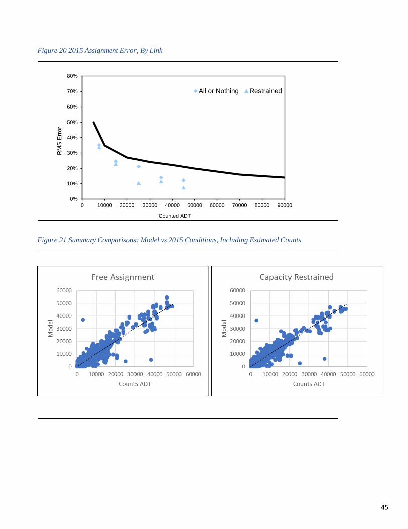
45

Figure 20 2015 Assignment Error, By Link

Figure 21 Summary Comparisons: Model vs 2015 Conditions, Including Estimated Counts

0%

10%

20%

30%

40%

50%

60%

70%

80%

0 10000 20000 30000 40000 50000 60000 70000 80000 90000

RM

S E

rro

r

Counted ADT

All or Nothing Restrained

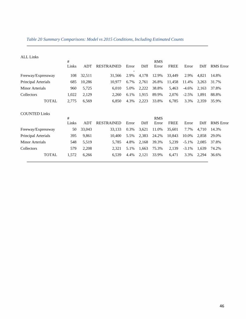
46

Table 20 Summary Comparisons: Model vs 2015 Conditions, Including Estimated Counts

ALL Links

#

Links ADT RESTRAINED Error Diff

RMS

Error FREE Error Diff RMS Error

Freeway/Expressway 108 32,511 31,566

-

2.9% 4,178 12.9% 33,449 2.9% 4,821 14.8%

Principal Arterials 685 10,286 10,977 6.7% 2,761 26.8% 11,458 11.4% 3,263 31.7%

Minor Arterials 960 5,725 6,010 5.0% 2,222 38.8% 5,463 -4.6% 2,163 37.8%

Collectors 1,022 2,129 2,260 6.1% 1,915 89.9% 2,076 -2.5% 1,891 88.8%

TOTAL 2,775 6,569 6,850 4.3% 2,223 33.8% 6,785 3.3% 2,359 35.9%

COUNTED Links

#

Links ADT RESTRAINED Error Diff

RMS

Error FREE Error Diff RMS Error

Freeway/Expressway 50 33,043 33,133 0.3% 3,621 11.0% 35,601 7.7% 4,710 14.3%

Principal Arterials 395 9,861 10,400 5.5% 2,383 24.2% 10,843 10.0% 2,858 29.0%

Minor Arterials 548 5,519 5,785 4.8% 2,168 39.3% 5,239 -5.1% 2,085 37.8%

Collectors 579 2,208 2,321 5.1% 1,663 75.3% 2,139 -3.1% 1,639 74.2%

TOTAL 1,572 6,266 6,539 4.4% 2,121 33.9% 6,471 3.3% 2,294 36.6%

47

48

Appendix A2 2015 Socio-Economic Data

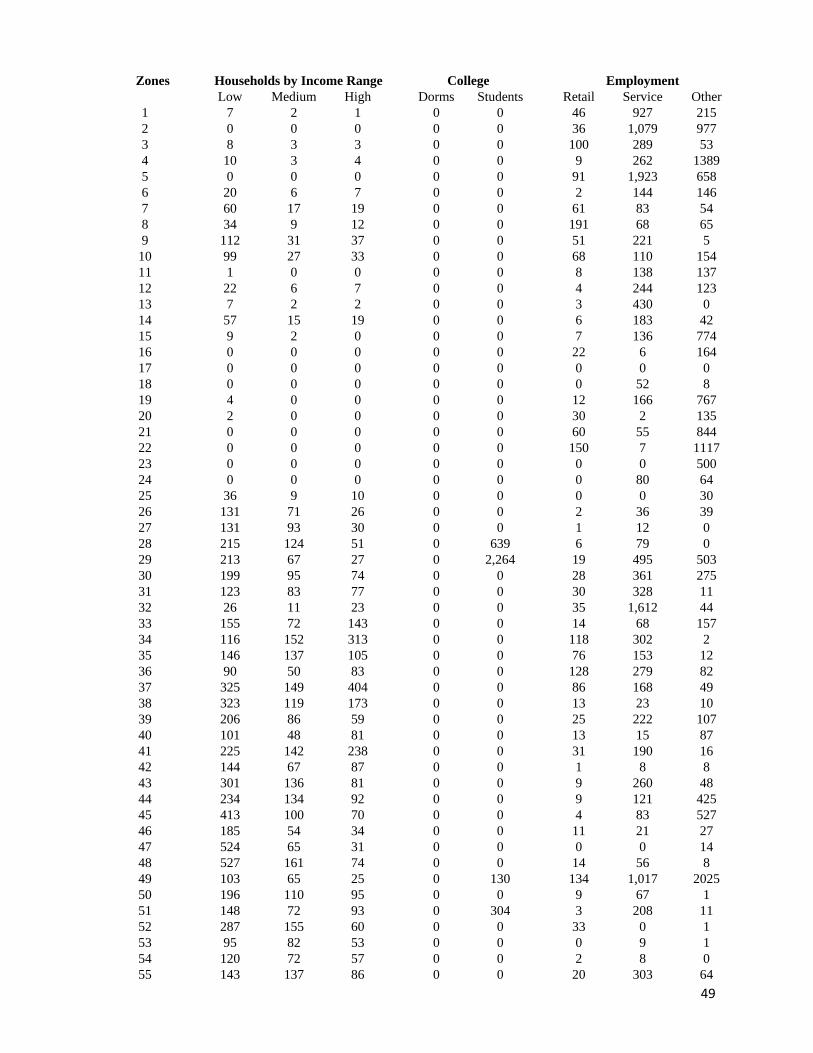
49

Zones Households by Income Range College Employment

Low Medium High Dorms Students Retail Service Other

1 7 2 1 0 0 46 927 215

2 0 0 0 0 0 36 1,079 977

3 8 3 3 0 0 100 289 53

4 10 3 4 0 0 9 262 1389

5 0 0 0 0 0 91 1,923 658

6 20 6 7 0 0 2 144 146

7 60 17 19 0 0 61 83 54

8 34 9 12 0 0 191 68 65

9 112 31 37 0 0 51 221 5

10 99 27 33 0 0 68 110 154

11 1 0 0 0 0 8 138 137

12 22 6 7 0 0 4 244 123

13 7 2 2 0 0 3 430 0

14 57 15 19 0 0 6 183 42

15 9 2 0 0 0 7 136 774

16 0 0 0 0 0 22 6 164

17 0 0 0 0 0 0 0 0

18 0 0 0 0 0 0 52 8

19 4 0 0 0 0 12 166 767

20 2 0 0 0 0 30 2 135

21 0 0 0 0 0 60 55 844

22 0 0 0 0 0 150 7 1117

23 0 0 0 0 0 0 0 500

24 0 0 0 0 0 0 80 64

25 36 9 10 0 0 0 0 30

26 131 71 26 0 0 2 36 39

27 131 93 30 0 0 1 12 0

28 215 124 51 0 639 6 79 0

29 213 67 27 0 2,264 19 495 503

30 199 95 74 0 0 28 361 275

31 123 83 77 0 0 30 328 11

32 26 11 23 0 0 35 1,612 44

33 155 72 143 0 0 14 68 157

34 116 152 313 0 0 118 302 2

35 146 137 105 0 0 76 153 12

36 90 50 83 0 0 128 279 82

37 325 149 404 0 0 86 168 49

38 323 119 173 0 0 13 23 10

39 206 86 59 0 0 25 222 107

40 101 48 81 0 0 13 15 87

41 225 142 238 0 0 31 190 16

42 144 67 87 0 0 1 8 8

43 301 136 81 0 0 9 260 48

44 234 134 92 0 0 9 121 425

45 413 100 70 0 0 4 83 527

46 185 54 34 0 0 11 21 27

47 524 65 31 0 0 0 0 14

48 527 161 74 0 0 14 56 8

49 103 65 25 0 130 134 1,017 2025

50 196 110 95 0 0 9 67 1

51 148 72 93 0 304 3 208 11

52 287 155 60 0 0 33 0 1

53 95 82 53 0 0 0 9 1

54 120 72 57 0 0 2 8 0

55 143 137 86 0 0 20 303 64

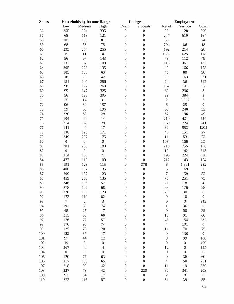
50

Zones Households by Income Range College Employment

Low Medium High Dorms Students Retail Service Other

56 355 324 335 0 0 29 128 209

57 68 118 121 0 0 247 610 164

58 107 106 81 0 0 66 111 74

59 68 53 75 0 0 704 86 18

60 293 254 255 0 0 192 214 28

61 15 11 4 0 0 1800 625 118

62 56 97 143 0 0 78 112 49

63 133 87 108 0 0 113 461 183

64 305 223 135 0 0 49 166 153

65 185 103 63 0 0 46 80 98

66 18 20 42 0 0 28 163 231

67 131 140 286 0 0 24 36 212

68 98 177 263 0 0 167 141 32

69 99 147 325 0 0 89 236 8

70 56 135 205 0 0 39 384 3

71 25 14 31 0 0 2 3,057 7

72 96 64 157 0 0 6 25 0

73 39 65 196 0 0 69 240 32

74 220 69 29 0 0 57 196 49

75 104 40 14 0 0 210 421 324

76 214 82 29 0 0 569 724 241

77 141 44 17 0 0 60 953 1202

78 138 198 171 0 0 42 151 27

79 349 207 175 0 0 11 53 23

80 0 0 0 0 0 1694 168 35

81 301 268 180 0 0 210 755 106

82 0 0 0 0 0 10 142 215

83 214 160 71 0 0 195 224 580

84 477 113 100 0 0 212 143 154

85 191 123 115 0 378 6 1,691 282

86 400 157 135 0 0 5 169 1

87 209 157 123 0 0 7 159 52

88 459 266 135 0 0 70 251 75

89 346 106 52 0 0 21 78 4

90 278 127 68 0 0 69 176 28

91 320 155 123 0 0 27 30 0

92 173 110 82 0 0 0 10 0

93 7 2 3 0 0 0 0 342

94 193 50 74 0 0 1 36 0

95 48 27 17 0 0 0 50 39

96 215 89 68 0 0 18 31 60

97 176 77 57 0 0 43 154 282

98 170 96 74 0 0 4 101 0

99 125 75 20 0 0 11 70 75

100 122 67 17 0 0 0 136 0

101 97 44 12 0 0 0 39 188

102 19 3 0 0 0 0 0 409

103 267 48 4 0 0 12 0 135

104 0 0 0 0 0 0 0 0

105 120 77 63 0 0 0 36 60

106 217 138 65 0 0 4 58 251

107 218 92 42 0 0 11 19 330

108 227 73 42 0 220 60 341 203

109 91 34 17 0 0 2 8 0

110 272 116 57 0 0 31 39 55

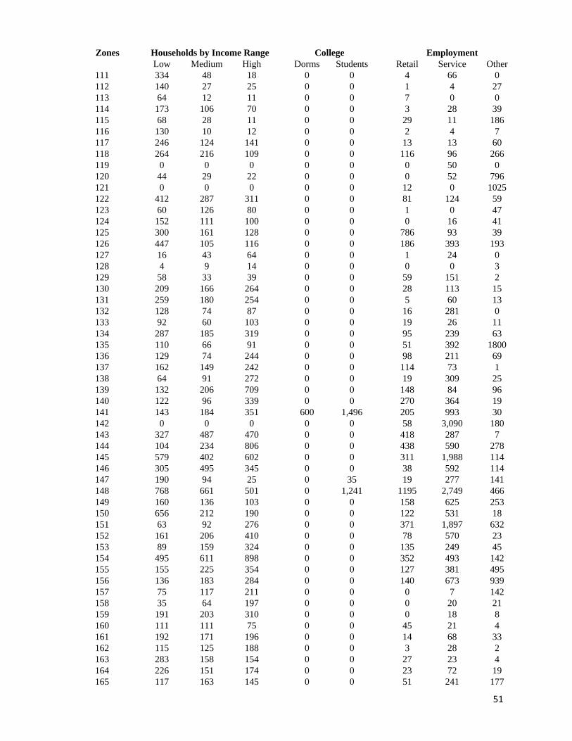
51

Zones Households by Income Range College Employment

Low Medium High Dorms Students Retail Service Other

111 334 48 18 0 0 4 66 0

112 140 27 25 0 0 1 4 27

113 64 12 11 0 0 7 0 0

114 173 106 70 0 0 3 28 39

115 68 28 11 0 0 29 11 186

116 130 10 12 0 0 2 4 7

117 246 124 141 0 0 13 13 60

118 264 216 109 0 0 116 96 266

119 0 0 0 0 0 0 50 0

120 44 29 22 0 0 0 52 796

121 0 0 0 0 0 12 0 1025

122 412 287 311 0 0 81 124 59

123 60 126 80 0 0 1 0 47

124 152 111 100 0 0 0 16 41

125 300 161 128 0 0 786 93 39

126 447 105 116 0 0 186 393 193

127 16 43 64 0 0 1 24 0

128 4 9 14 0 0 0 0 3

129 58 33 39 0 0 59 151 2

130 209 166 264 0 0 28 113 15

131 259 180 254 0 0 5 60 13

132 128 74 87 0 0 16 281 0

133 92 60 103 0 0 19 26 11

134 287 185 319 0 0 95 239 63

135 110 66 91 0 0 51 392 1800

136 129 74 244 0 0 98 211 69

137 162 149 242 0 0 114 73 1

138 64 91 272 0 0 19 309 25

139 132 206 709 0 0 148 84 96

140 122 96 339 0 0 270 364 19

141 143 184 351 600 1,496 205 993 30

142 0 0 0 0 0 58 3,090 180

143 327 487 470 0 0 418 287 7

144 104 234 806 0 0 438 590 278

145 579 402 602 0 0 311 1,988 114

146 305 495 345 0 0 38 592 114

147 190 94 25 0 35 19 277 141

148 768 661 501 0 1,241 1195 2,749 466

149 160 136 103 0 0 158 625 253

150 656 212 190 0 0 122 531 18

151 63 92 276 0 0 371 1,897 632

152 161 206 410 0 0 78 570 23

153 89 159 324 0 0 135 249 45

154 495 611 898 0 0 352 493 142

155 155 225 354 0 0 127 381 495

156 136 183 284 0 0 140 673 939

157 75 117 211 0 0 0 7 142

158 35 64 197 0 0 0 20 21

159 191 203 310 0 0 0 18 8

160 111 111 75 0 0 45 21 4

161 192 171 196 0 0 14 68 33

162 115 125 188 0 0 3 28 2

163 283 158 154 0 0 27 23 4

164 226 151 174 0 0 23 72 19

165 117 163 145 0 0 51 241 177

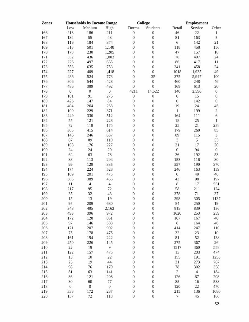
52

Zones Households by Income Range College Employment

Low Medium High Dorms Students Retail Service Other

166 213 186 211 0 0 46 22 1

167 134 55 43 0 0 81 163 5

168 116 184 374 0 0 6 142 21

169 313 501 1,148 0 0 118 458 156

170 173 230 1,205 0 0 47 157 18

171 552 436 1,003 0 0 76 497 24

172 226 497 665 0 0 86 417 11

173 553 635 753 0 0 241 458 24

174 227 409 1,418 0 0 1018 1,935 49

175 486 524 773 0 35 375 5,947 100

176 806 544 428 0 0 460 248 46

177 486 389 492 0 0 169 613 20

178 0 0 0 4211 14,522 140 2,596 0

179 161 91 275 0 0 0 15 0

180 426 147 84 0 0 0 142 0

181 404 264 253 0 0 19 24 45

182 109 229 371 0 0 1 199 2

183 249 330 512 0 0 164 111 6

184 55 121 228 0 0 18 25 1

185 72 118 175 0 0 25 21 238

186 305 415 614 0 0 179 260 85

187 146 246 637 0 0 89 115 3

188 87 89 110 0 0 3 5 53

189 168 176 227 0 0 21 17 20

190 24 24 29 0 0 0 94 0

191 62 63 78 0 0 36 192 53

192 88 113 294 0 0 153 116 80

193 99 129 335 0 0 557 190 370

194 174 224 528 0 0 246 163 139

195 109 201 475 0 0 0 49 46

196 385 389 455 0 0 43 98 197

197 11 4 4 0 0 8 17 551

198 217 95 72 0 0 58 211 124

199 35 32 43 0 0 378 71 37

200 15 13 19 0 0 298 305 1137

201 95 209 680 0 0 54 250 19

202 348 495 2,162 0 0 815 839 136

203 493 396 972 0 0 1620 253 259

204 172 128 851 0 0 167 167 40

205 97 146 583 0 0 8 164 46

206 171 207 902 0 0 414 247 110

207 75 178 475 0 0 32 23 10

208 161 194 222 0 0 81 52 138

209 250 226 145 0 0 275 367 26

210 22 19 9 0 0 1517 360 558

211 122 157 475 0 0 15 203 474

212 13 10 22 0 0 155 191 1258

213 25 19 44 0 0 21 273 767

214 98 76 170 0 0 78 302 358

215 81 63 141 0 0 2 4 184

216 86 121 208 0 0 126 67 208

217 30 60 77 0 0 85 16 538

218 0 0 0 0 0 120 22 470

219 333 172 287 0 0 215 136 1080

220 137 72 118 0 0 7 45 166

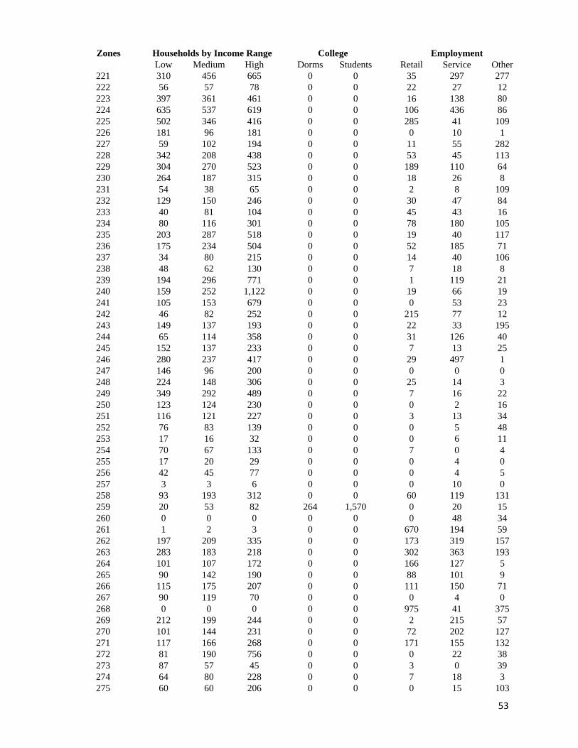
53

Zones Households by Income Range College Employment

Low Medium High Dorms Students Retail Service Other

221 310 456 665 0 0 35 297 277

222 56 57 78 0 0 22 27 12

223 397 361 461 0 0 16 138 80

224 635 537 619 0 0 106 436 86

225 502 346 416 0 0 285 41 109

226 181 96 181 0 0 0 10 1

227 59 102 194 0 0 11 55 282

228 342 208 438 0 0 53 45 113

229 304 270 523 0 0 189 110 64

230 264 187 315 0 0 18 26 8

231 54 38 65 0 0 2 8 109

232 129 150 246 0 0 30 47 84

233 40 81 104 0 0 45 43 16

234 80 116 301 0 0 78 180 105

235 203 287 518 0 0 19 40 117

236 175 234 504 0 0 52 185 71

237 34 80 215 0 0 14 40 106

238 48 62 130 0 0 7 18 8

239 194 296 771 0 0 1 119 21

240 159 252 1,122 0 0 19 66 19

241 105 153 679 0 0 0 53 23

242 46 82 252 0 0 215 77 12

243 149 137 193 0 0 22 33 195

244 65 114 358 0 0 31 126 40

245 152 137 233 0 0 7 13 25

246 280 237 417 0 0 29 497 1

247 146 96 200 0 0 0 0 0

248 224 148 306 0 0 25 14 3

249 349 292 489 0 0 7 16 22

250 123 124 230 0 0 0 2 16

251 116 121 227 0 0 3 13 34

252 76 83 139 0 0 0 5 48

253 17 16 32 0 0 0 6 11

254 70 67 133 0 0 7 0 4

255 17 20 29 0 0 0 4 0

256 42 45 77 0 0 0 4 5

257 3 3 6 0 0 0 10 0

258 93 193 312 0 0 60 119 131

259 20 53 82 264 1,570 0 20 15

260 0 0 0 0 0 0 48 34

261 1 2 3 0 0 670 194 59

262 197 209 335 0 0 173 319 157

263 283 183 218 0 0 302 363 193

264 101 107 172 0 0 166 127 5

265 90 142 190 0 0 88 101 9

266 115 175 207 0 0 111 150 71

267 90 119 70 0 0 0 4 0

268 0 0 0 0 0 975 41 375

269 212 199 244 0 0 2 215 57

270 101 144 231 0 0 72 202 127

271 117 166 268 0 0 171 155 132

272 81 190 756 0 0 0 22 38

273 87 57 45 0 0 3 0 39

274 64 80 228 0 0 7 18 3

275 60 60 206 0 0 0 15 103

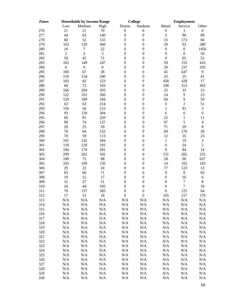
54

Zones Households by Income Range College Employment

Low Medium High Dorms Students Retail Service Other

276 21 21 70 0 0 0 3 0

277 44 63 140 0 0 5 90 89

278 60 52 155 0 0 15 173 66

279 163 129 368 0 0 29 93 280

280 10 7 22 0 0 0 0 1456

281 2 2 3 0 0 0 0 50

282 59 42 71 0 0 0 65 52

283 162 149 247 0 0 59 155 410

284 0 0 0 0 0 20 237 203

285 100 67 28 0 0 45 647 9

286 119 154 240 0 0 25 35 41

287 103 82 123 0 0 458 428 17

288 68 72 103 0 0 108 313 493

289 166 204 293 0 0 25 33 13

290 122 161 266 0 0 14 9 23

291 129 109 184 0 0 66 9 50

292 63 63 214 0 0 0 2 51

293 156 56 153 0 0 2 81 2

294 93 129 304 0 0 6 0 6

295 66 81 220 0 0 22 1 11

296 90 74 127 0 0 97 5 4

297 29 25 59 0 0 71 20 8

298 70 64 152 0 0 69 176 26

299 70 59 113 0 0 12 35 23

300 101 142 204 0 0 2 19 3

301 118 120 193 0 0 0 24 5

302 194 174 281 0 0 9 84 14

303 299 162 102 0 0 131 265 255

304 108 75 88 0 0 28 90 637

305 103 109 150 0 0 14 102 183

306 29 23 24 0 0 77 123 13

307 83 66 71 0 0 9 8 93

308 19 15 17 0 0 0 16 6

309 31 27 51 0 0 0 7 8

310 24 44 105 0 0 0 7 50

311 78 137 383 0 0 0 125 64

312 17 15 18 0 0 105 217 170

313 N/A N/A N/A N/A N/A N/A N/A N/A

314 N/A N/A N/A N/A N/A N/A N/A N/A

315 N/A N/A N/A N/A N/A N/A N/A N/A

316 N/A N/A N/A N/A N/A N/A N/A N/A

317 N/A N/A N/A N/A N/A N/A N/A N/A

318 N/A N/A N/A N/A N/A N/A N/A N/A

319 N/A N/A N/A N/A N/A N/A N/A N/A

320 N/A N/A N/A N/A N/A N/A N/A N/A

321 N/A N/A N/A N/A N/A N/A N/A N/A

322 N/A N/A N/A N/A N/A N/A N/A N/A

323 N/A N/A N/A N/A N/A N/A N/A N/A

324 N/A N/A N/A N/A N/A N/A N/A N/A

325 N/A N/A N/A N/A N/A N/A N/A N/A

326 N/A N/A N/A N/A N/A N/A N/A N/A

327 N/A N/A N/A N/A N/A N/A N/A N/A

328 N/A N/A N/A N/A N/A N/A N/A N/A

329 N/A N/A N/A N/A N/A N/A N/A N/A

330 N/A N/A N/A N/A N/A N/A N/A N/A

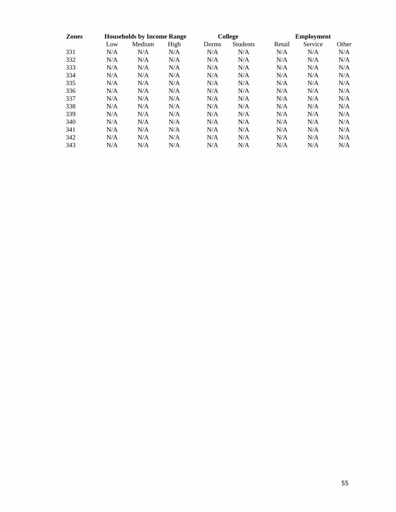
55

Zones Households by Income Range College Employment

Low Medium High Dorms Students Retail Service Other

331 N/A N/A N/A N/A N/A N/A N/A N/A

332 N/A N/A N/A N/A N/A N/A N/A N/A

333 N/A N/A N/A N/A N/A N/A N/A N/A

334 N/A N/A N/A N/A N/A N/A N/A N/A

335 N/A N/A N/A N/A N/A N/A N/A N/A

336 N/A N/A N/A N/A N/A N/A N/A N/A

337 N/A N/A N/A N/A N/A N/A N/A N/A

338 N/A N/A N/A N/A N/A N/A N/A N/A

339 N/A N/A N/A N/A N/A N/A N/A N/A

340 N/A N/A N/A N/A N/A N/A N/A N/A

341 N/A N/A N/A N/A N/A N/A N/A N/A

342 N/A N/A N/A N/A N/A N/A N/A N/A

343 N/A N/A N/A N/A N/A N/A N/A N/A

56

Appendix A3 2045 Socio-

economic Data

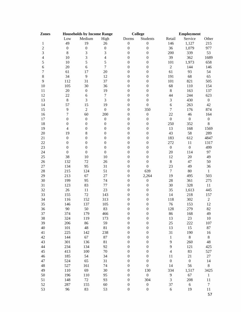
57

Zones Households by Income Range College Employment

Low Medium High Dorms Students Retail Service Other

1 49 19 26 0 0 146 1,127 215

2 0 0 0 0 0 36 1,079 977

3 8 3 3 0 0 200 339 53

4 10 3 4 0 0 39 362 1689

5 10 5 5 0 0 101 1,973 658

6 20 6 7 0 0 2 144 146

7 61 17 20 0 0 61 93 54

8 34 9 12 0 0 191 68 65

9 112 31 37 0 0 101 821 505

10 105 30 36 0 0 68 110 154

11 20 0 19 0 0 8 163 137

12 22 6 7 0 0 44 244 623

13 8 3 3 0 0 3 430 0

14 57 15 19 0 0 6 263 42

15 9 2 0 0 350 7 176 874

16 7 60 200 0 0 22 46 164

17 0 0 0 0 0 0 0 0

18 0 0 0 0 0 250 352 8

19 4 0 0 0 0 13 168 1569

20 19 8 0 0 0 43 58 289

21 0 0 0 0 0 183 612 4847

22 0 0 0 0 0 272 11 1317

23 0 0 0 0 0 0 0 499

24 0 0 0 0 0 20 114 97

25 38 10 10 0 0 12 20 49

26 132 72 26 0 0 8 47 50

27 134 95 31 0 0 23 49 36

28 215 124 51 0 639 7 80 1

29 213 67 27 0 2,264 19 495 503

30 199 95 74 0 0 28 361 275

31 123 83 77 0 0 30 328 11

32 26 11 23 0 0 35 1,613 445

33 155 72 143 0 0 14 218 157

34 116 152 313 0 0 118 302 2

35 146 137 105 0 0 76 153 12

36 90 50 83 0 0 128 279 82

37 374 179 466 0 0 86 168 49

38 324 119 173 0 0 13 23 10

39 206 86 59 0 0 25 222 107

40 101 48 81 0 0 13 15 87

41 225 142 238 0 0 31 190 16

42 144 67 87 0 0 1 8 8

43 301 136 81 0 0 9 260 48

44 234 134 92 0 0 9 121 425

45 413 100 70 0 0 4 83 527

46 185 54 34 0 0 11 21 27

47 524 65 31 0 0 0 0 14

48 527 161 74 0 0 14 56 8

49 110 69 30 0 130 334 1,517 3425

50 196 110 95 0 0 9 67 1

51 148 72 93 0 304 3 208 11

52 287 155 60 0 0 37 6 7

53 96 83 53 0 0 6 19 11

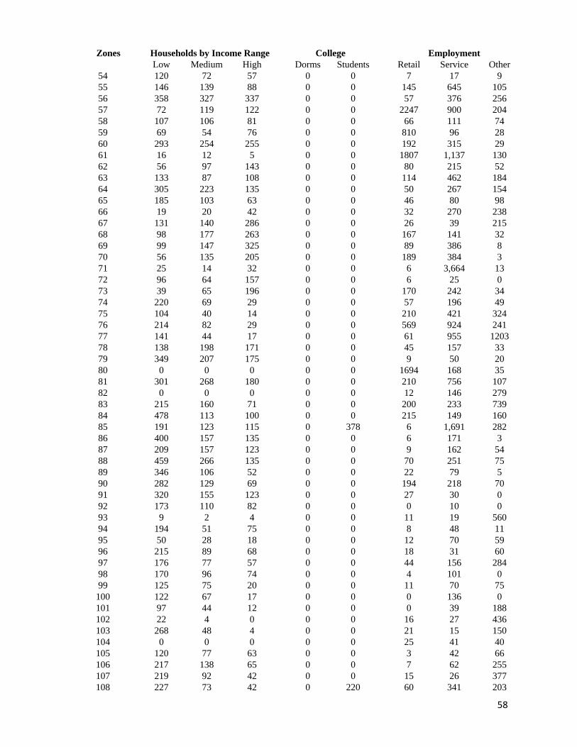
58

Zones Households by Income Range College Employment

Low Medium High Dorms Students Retail Service Other

54 120 72 57 0 0 7 17 9

55 146 139 88 0 0 145 645 105

56 358 327 337 0 0 57 376 256

57 72 119 122 0 0 2247 900 204

58 107 106 81 0 0 66 111 74

59 69 54 76 0 0 810 96 28

60 293 254 255 0 0 192 315 29

61 16 12 5 0 0 1807 1,137 130

62 56 97 143 0 0 80 215 52

63 133 87 108 0 0 114 462 184

64 305 223 135 0 0 50 267 154

65 185 103 63 0 0 46 80 98

66 19 20 42 0 0 32 270 238

67 131 140 286 0 0 26 39 215

68 98 177 263 0 0 167 141 32

69 99 147 325 0 0 89 386 8

70 56 135 205 0 0 189 384 3

71 25 14 32 0 0 6 3,664 13

72 96 64 157 0 0 6 25 0

73 39 65 196 0 0 170 242 34

74 220 69 29 0 0 57 196 49

75 104 40 14 0 0 210 421 324

76 214 82 29 0 0 569 924 241

77 141 44 17 0 0 61 955 1203

78 138 198 171 0 0 45 157 33

79 349 207 175 0 0 9 50 20

80 0 0 0 0 0 1694 168 35

81 301 268 180 0 0 210 756 107

82 0 0 0 0 0 12 146 279

83 215 160 71 0 0 200 233 739

84 478 113 100 0 0 215 149 160

85 191 123 115 0 378 6 1,691 282

86 400 157 135 0 0 6 171 3

87 209 157 123 0 0 9 162 54

88 459 266 135 0 0 70 251 75

89 346 106 52 0 0 22 79 5

90 282 129 69 0 0 194 218 70

91 320 155 123 0 0 27 30 0

92 173 110 82 0 0 0 10 0

93 9 2 4 0 0 11 19 560

94 194 51 75 0 0 8 48 11

95 50 28 18 0 0 12 70 59

96 215 89 68 0 0 18 31 60

97 176 77 57 0 0 44 156 284

98 170 96 74 0 0 4 101 0

99 125 75 20 0 0 11 70 75

100 122 67 17 0 0 0 136 0

101 97 44 12 0 0 0 39 188

102 22 4 0 0 0 16 27 436

103 268 48 4 0 0 21 15 150

104 0 0 0 0 0 25 41 40

105 120 77 63 0 0 3 42 66

106 217 138 65 0 0 7 62 255

107 219 92 42 0 0 15 26 377

108 227 73 42 0 220 60 341 203

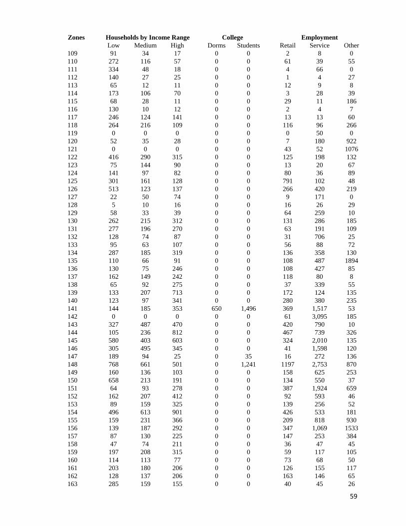
59

Zones Households by Income Range College Employment

Low Medium High Dorms Students Retail Service Other

109 91 34 17 0 0 2 8 0

110 272 116 57 0 0 61 39 55

111 334 48 18 0 0 4 66 0

112 140 27 25 0 0 1 4 27

113 65 12 11 0 0 12 9 8

114 173 106 70 0 0 3 28 39

115 68 28 11 0 0 29 11 186

116 130 10 12 0 0 2 4 7

117 246 124 141 0 0 13 13 60

118 264 216 109 0 0 116 96 266

119 0 0 0 0 0 0 50 0

120 52 35 28 0 0 7 180 922

121 0 0 0 0 0 43 52 1076

122 416 290 315 0 0 125 198 132

123 75 144 90 0 0 13 20 67

124 141 97 82 0 0 80 36 89

125 301 161 128 0 0 791 102 48

126 513 123 137 0 0 266 420 219

127 22 50 74 0 0 9 171 0

128 5 10 16 0 0 16 26 29

129 58 33 39 0 0 64 259 10

130 262 215 312 0 0 131 286 185

131 277 196 270 0 0 63 191 109

132 128 74 87 0 0 31 706 25

133 95 63 107 0 0 56 88 72

134 287 185 319 0 0 136 358 130

135 110 66 91 0 0 108 487 1894

136 130 75 246 0 0 108 427 85

137 162 149 242 0 0 118 80 8

138 65 92 275 0 0 37 339 55

139 133 207 713 0 0 172 124 135

140 123 97 341 0 0 280 380 235

141 144 185 353 650 1,496 369 1,517 53

142 0 0 0 0 0 61 3,095 185

143 327 487 470 0 0 420 790 10

144 105 236 812 0 0 467 739 326

145 580 403 603 0 0 324 2,010 135

146 305 495 345 0 0 41 1,598 120

147 189 94 25 0 35 16 272 136

148 768 661 501 0 1,241 1197 2,753 870

149 160 136 103 0 0 158 625 253

150 658 213 191 0 0 134 550 37

151 64 93 278 0 0 387 1,924 659

152 162 207 412 0 0 92 593 46

153 89 159 325 0 0 139 256 52

154 496 613 901 0 0 426 533 181

155 159 231 366 0 0 209 818 930

156 139 187 292 0 0 347 1,069 1533

157 87 130 225 0 0 147 253 384

158 47 74 211 0 0 36 47 45

159 197 208 315 0 0 59 117 105

160 114 113 77 0 0 73 68 50

161 203 180 206 0 0 126 155 117

162 128 137 206 0 0 163 146 65

163 285 159 155 0 0 40 45 26

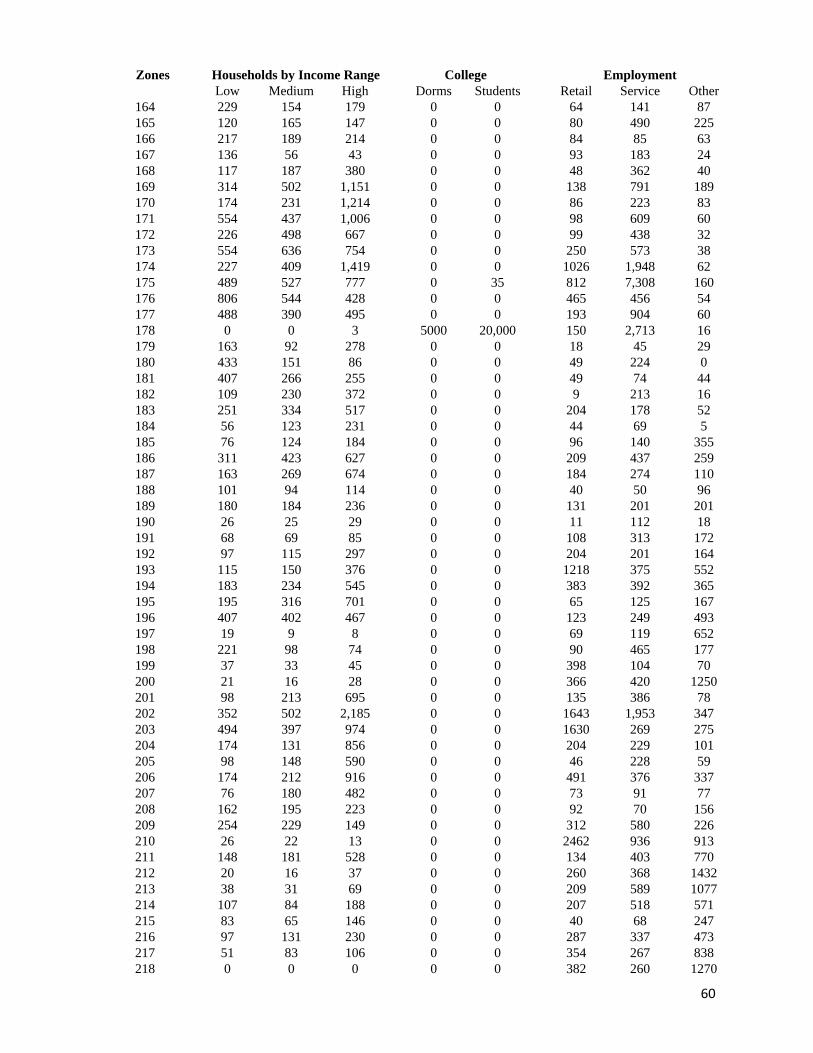
60

Zones Households by Income Range College Employment

Low Medium High Dorms Students Retail Service Other

164 229 154 179 0 0 64 141 87

165 120 165 147 0 0 80 490 225

166 217 189 214 0 0 84 85 63

167 136 56 43 0 0 93 183 24

168 117 187 380 0 0 48 362 40

169 314 502 1,151 0 0 138 791 189

170 174 231 1,214 0 0 86 223 83

171 554 437 1,006 0 0 98 609 60

172 226 498 667 0 0 99 438 32

173 554 636 754 0 0 250 573 38

174 227 409 1,419 0 0 1026 1,948 62

175 489 527 777 0 35 812 7,308 160

176 806 544 428 0 0 465 456 54

177 488 390 495 0 0 193 904 60

178 0 0 3 5000 20,000 150 2,713 16

179 163 92 278 0 0 18 45 29

180 433 151 86 0 0 49 224 0

181 407 266 255 0 0 49 74 44

182 109 230 372 0 0 9 213 16

183 251 334 517 0 0 204 178 52

184 56 123 231 0 0 44 69 5

185 76 124 184 0 0 96 140 355

186 311 423 627 0 0 209 437 259

187 163 269 674 0 0 184 274 110

188 101 94 114 0 0 40 50 96

189 180 184 236 0 0 131 201 201

190 26 25 29 0 0 11 112 18

191 68 69 85 0 0 108 313 172

192 97 115 297 0 0 204 201 164

193 115 150 376 0 0 1218 375 552

194 183 234 545 0 0 383 392 365

195 195 316 701 0 0 65 125 167

196 407 402 467 0 0 123 249 493

197 19 9 8 0 0 69 119 652

198 221 98 74 0 0 90 465 177

199 37 33 45 0 0 398 104 70

200 21 16 28 0 0 366 420 1250

201 98 213 695 0 0 135 386 78

202 352 502 2,185 0 0 1643 1,953 347

203 494 397 974 0 0 1630 269 275

204 174 131 856 0 0 204 229 101

205 98 148 590 0 0 46 228 59

206 174 212 916 0 0 491 376 337

207 76 180 482 0 0 73 91 77

208 162 195 223 0 0 92 70 156

209 254 229 149 0 0 312 580 226

210 26 22 13 0 0 2462 936 913

211 148 181 528 0 0 134 403 770

212 20 16 37 0 0 260 368 1432

213 38 31 69 0 0 209 589 1077

214 107 84 188 0 0 207 518 571

215 83 65 146 0 0 40 68 247

216 97 131 230 0 0 287 337 473

217 51 83 106 0 0 354 267 838

218 0 0 0 0 0 382 260 1270

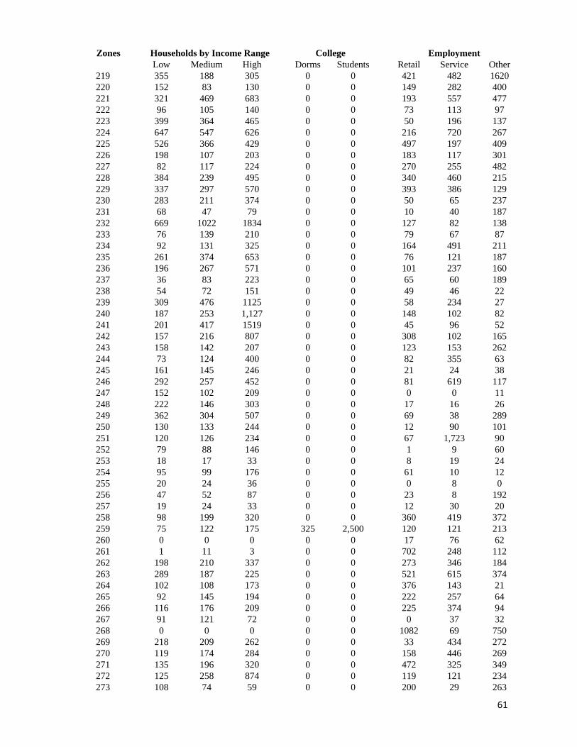
61

Zones Households by Income Range College Employment

Low Medium High Dorms Students Retail Service Other

219 355 188 305 0 0 421 482 1620

220 152 83 130 0 0 149 282 400

221 321 469 683 0 0 193 557 477

222 96 105 140 0 0 73 113 97

223 399 364 465 0 0 50 196 137

224 647 547 626 0 0 216 720 267

225 526 366 429 0 0 497 197 409

226 198 107 203 0 0 183 117 301

227 82 117 224 0 0 270 255 482

228 384 239 495 0 0 340 460 215

229 337 297 570 0 0 393 386 129

230 283 211 374 0 0 50 65 237

231 68 47 79 0 0 10 40 187

232 669 1022 1834 0 0 127 82 138

233 76 139 210 0 0 79 67 87

234 92 131 325 0 0 164 491 211

235 261 374 653 0 0 76 121 187

236 196 267 571 0 0 101 237 160

237 36 83 223 0 0 65 60 189

238 54 72 151 0 0 49 46 22

239 309 476 1125 0 0 58 234 27

240 187 253 1,127 0 0 148 102 82

241 201 417 1519 0 0 45 96 52

242 157 216 807 0 0 308 102 165

243 158 142 207 0 0 123 153 262

244 73 124 400 0 0 82 355 63

245 161 145 246 0 0 21 24 38

246 292 257 452 0 0 81 619 117

247 152 102 209 0 0 0 0 11

248 222 146 303 0 0 17 16 26

249 362 304 507 0 0 69 38 289

250 130 133 244 0 0 12 90 101

251 120 126 234 0 0 67 1,723 90

252 79 88 146 0 0 1 9 60

253 18 17 33 0 0 8 19 24

254 95 99 176 0 0 61 10 12

255 20 24 36 0 0 0 8 0

256 47 52 87 0 0 23 8 192

257 19 24 33 0 0 12 30 20

258 98 199 320 0 0 360 419 372

259 75 122 175 325 2,500 120 121 213

260 0 0 0 0 0 17 76 62

261 1 11 3 0 0 702 248 112

262 198 210 337 0 0 273 346 184

263 289 187 225 0 0 521 615 374

264 102 108 173 0 0 376 143 21

265 92 145 194 0 0 222 257 64

266 116 176 209 0 0 225 374 94

267 91 121 72 0 0 0 37 32

268 0 0 0 0 0 1082 69 750

269 218 209 262 0 0 33 434 272

270 119 174 284 0 0 158 446 269

271 135 196 320 0 0 472 325 349

272 125 258 874 0 0 119 121 234

273 108 74 59 0 0 200 29 263

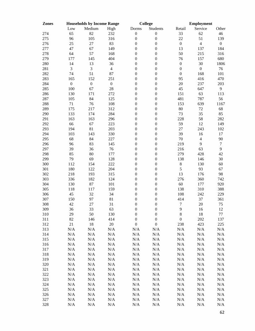
62

Zones Households by Income Range College Employment

Low Medium High Dorms Students Retail Service Other

274 65 82 232 0 0 33 62 46

275 96 105 316 0 0 22 51 139

276 25 27 83 0 0 0 4 0

277 47 67 149 0 0 13 137 184

278 64 57 168 0 0 50 215 316

279 177 145 404 0 0 76 157 680

280 14 13 36 0 0 0 30 1806

281 3 3 4 0 0 0 0 76

282 74 51 87 0 0 0 168 101

283 165 152 251 0 0 95 416 470

284 0 0 0 0 0 20 237 203

285 100 67 28 0 0 45 647 9

286 130 171 272 0 0 151 63 113

287 105 84 125 0 0 481 787 56

288 71 76 108 0 0 153 639 1167

289 175 217 312 0 0 80 72 68

290 133 174 284 0 0 73 35 85

291 163 163 296 0 0 228 58 282

292 66 67 223 0 0 59 12 149

293 194 81 203 0 0 27 243 102

294 103 143 330 0 0 39 16 17

295 68 84 227 0 0 70 4 90

296 96 83 145 0 0 219 9 7

297 39 36 76 0 0 216 63 9

298 85 80 177 0 0 279 428 42

299 79 69 128 0 0 138 146 30

300 112 154 222 0 0 8 130 60

301 180 122 204 0 0 5 93 67

302 218 193 315 0 0 13 176 98

303 336 182 124 0 0 276 360 742

304 130 87 101 0 0 60 177 920

305 118 117 159 0 0 138 310 388

306 45 32 34 0 0 108 242 229

307 150 97 81 0 0 414 37 361

308 42 27 31 0 0 7 20 75

309 36 33 63 0 0 9 16 12

310 29 50 130 0 0 8 18 77

311 82 146 414 0 0 0 202 137

312 21 18 20 0 0 238 423 225

313 N/A N/A N/A N/A N/A N/A N/A N/A

314 N/A N/A N/A N/A N/A N/A N/A N/A

315 N/A N/A N/A N/A N/A N/A N/A N/A

316 N/A N/A N/A N/A N/A N/A N/A N/A

317 N/A N/A N/A N/A N/A N/A N/A N/A

318 N/A N/A N/A N/A N/A N/A N/A N/A

319 N/A N/A N/A N/A N/A N/A N/A N/A

320 N/A N/A N/A N/A N/A N/A N/A N/A

321 N/A N/A N/A N/A N/A N/A N/A N/A

322 N/A N/A N/A N/A N/A N/A N/A N/A

323 N/A N/A N/A N/A N/A N/A N/A N/A

324 N/A N/A N/A N/A N/A N/A N/A N/A

325 N/A N/A N/A N/A N/A N/A N/A N/A

326 N/A N/A N/A N/A N/A N/A N/A N/A

327 N/A N/A N/A N/A N/A N/A N/A N/A

328 N/A N/A N/A N/A N/A N/A N/A N/A

63

Zones Households by Income Range College Employment

Low Medium High Dorms Students Retail Service Other

329 N/A N/A N/A N/A N/A N/A N/A N/A

330 N/A N/A N/A N/A N/A N/A N/A N/A

331 N/A N/A N/A N/A N/A N/A N/A N/A

332 N/A N/A N/A N/A N/A N/A N/A N/A

333 N/A N/A N/A N/A N/A N/A N/A N/A

334 N/A N/A N/A N/A N/A N/A N/A N/A

335 N/A N/A N/A N/A N/A N/A N/A N/A

336 N/A N/A N/A N/A N/A N/A N/A N/A

337 N/A N/A N/A N/A N/A N/A N/A N/A

338 N/A N/A N/A N/A N/A N/A N/A N/A

339 N/A N/A N/A N/A N/A N/A N/A N/A

340 N/A N/A N/A N/A N/A N/A N/A N/A

341 N/A N/A N/A N/A N/A N/A N/A N/A

342 N/A N/A N/A N/A N/A N/A N/A N/A

343 N/A N/A N/A N/A N/A N/A N/A N/A

64

Appendix A4 2015 Trip Ends

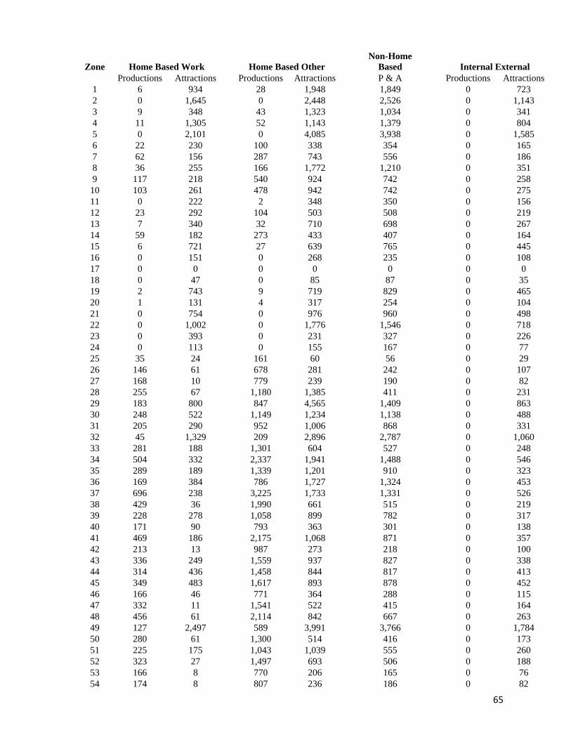
65

Zone Home Based Work Home Based Other

Non-Home

Based Internal External

Productions Attractions Productions Attractions P & A Productions Attractions

1 6 934 28 1,948 1,849 0 723

2 0 1,645 0 2,448 2,526 0 1,143

3 9 348 43 1,323 1,034 0 341

4 11 1,305 52 1,143 1,379 0 804

5 0 2,101 0 4,085 3,938 0 1,585

6 22 230 100 338 354 0 165

7 62 156 287 743 556 0 186

8 36 255 166 1,772 1,210 0 351

9 117 218 540 924 742 0 258

10 103 261 478 942 742 0 275

11 0 222 2 348 350 0 156

12 23 292 104 503 508 0 219

13 7 340 32 710 698 0 267

14 59 182 273 433 407 0 164

15 6 721 27 639 765 0 445

16 0 151 0 268 235 0 108

17 0 0 0 0 0 0 0

18 0 47 0 85 87 0 35

19 2 743 9 719 829 0 465

20 1 131 4 317 254 0 104

21 0 754 0 976 960 0 498

22 0 1,002 0 1,776 1,546 0 718

23 0 393 0 231 327 0 226

24 0 113 0 155 167 0 77

25 35 24 161 60 56 0 29

26 146 61 678 281 242 0 107

27 168 10 779 239 190 0 82

28 255 67 1,180 1,385 411 0 231

29 183 800 847 4,565 1,409 0 863

30 248 522 1,149 1,234 1,138 0 488

31 205 290 952 1,006 868 0 331

32 45 1,329 209 2,896 2,787 0 1,060

33 281 188 1,301 604 527 0 248

34 504 332 2,337 1,941 1,488 0 546

35 289 189 1,339 1,201 910 0 323

36 169 384 786 1,727 1,324 0 453

37 696 238 3,225 1,733 1,331 0 526

38 429 36 1,990 661 515 0 219

39 228 278 1,058 899 782 0 317

40 171 90 793 363 301 0 138

41 469 186 2,175 1,068 871 0 357

42 213 13 987 273 218 0 100

43 336 249 1,559 937 827 0 338

44 314 436 1,458 844 817 0 413

45 349 483 1,617 893 878 0 452

46 166 46 771 364 288 0 115

47 332 11 1,541 522 415 0 164

48 456 61 2,114 842 667 0 263

49 127 2,497 589 3,991 3,766 0 1,784

50 280 61 1,300 514 416 0 173

51 225 175 1,043 1,039 555 0 260

52 323 27 1,497 693 506 0 188

53 166 8 770 206 165 0 76

54 174 8 807 236 186 0 82

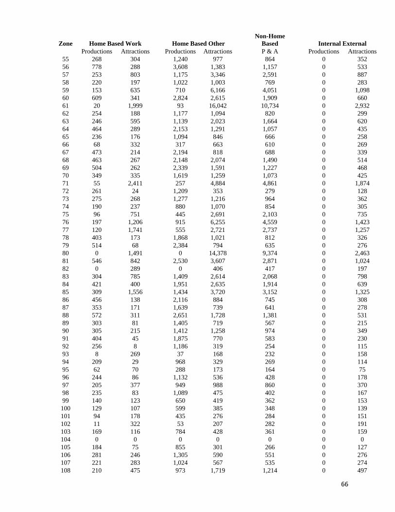
66

Zone Home Based Work Home Based Other

Non-Home

Based Internal External

Productions Attractions Productions Attractions P & A Productions Attractions

55 268 304 1,240 977 864 0 352

56 778 288 3,608 1,383 1,157 0 533

57 253 803 1,175 3,346 2,591 0 887

58 220 197 1,022 1,003 769 0 283

59 153 635 710 6,166 4,051 0 1,098

60 609 341 2,824 2,615 1,909 0 660

61 20 1,999 93 16,042 10,734 0 2,932

62 254 188 1,177 1,094 820 0 299

63 246 595 1,139 2,023 1,664 0 620

64 464 289 2,153 1,291 1,057 0 435

65 236 176 1,094 846 666 0 258

66 68 332 317 663 610 0 269

67 473 214 2,194 818 688 0 339

68 463 267 2,148 2,074 1,490 0 514

69 504 262 2,339 1,591 1,227 0 468

70 349 335 1,619 1,259 1,073 0 425

71 55 2,411 257 4,884 4,861 0 1,874

72 261 24 1,209 353 279 0 128

73 275 268 1,277 1,216 964 0 362

74 190 237 880 1,070 854 0 305

75 96 751 445 2,691 2,103 0 735

76 197 1,206 915 6,255 4,559 0 1,423

77 120 1,741 555 2,721 2,737 0 1,257

78 403 173 1,868 1,021 812 0 326

79 514 68 2,384 794 635 0 276

80 0 1,491 0 14,378 9,374 0 2,463

81 546 842 2,530 3,607 2,871 0 1,024

82 0 289 0 406 417 0 197

83 304 785 1,409 2,614 2,068 0 798

84 421 400 1,951 2,635 1,914 0 639

85 309 1,556 1,434 3,720 3,152 0 1,325

86 456 138 2,116 884 745 0 308

87 353 171 1,639 739 641 0 278

88 572 311 2,651 1,728 1,381 0 531

89 303 81 1,405 719 567 0 215

90 305 215 1,412 1,258 974 0 349

91 404 45 1,875 770 583 0 230

92 256 8 1,186 319 254 0 115

93 8 269 37 168 232 0 158

94 209 29 968 329 269 0 114

95 62 70 288 173 164 0 75

96 244 86 1,132 536 428 0 178

97 205 377 949 988 860 0 370

98 235 83 1,089 475 402 0 167

99 140 123 650 419 362 0 153

100 129 107 599 385 348 0 139

101 94 178 435 276 284 0 151

102 11 322 53 207 282 0 191

103 169 116 784 428 361 0 159

104 0 0 0 0 0 0 0

105 184 75 855 301 266 0 127

106 281 246 1,305 590 551 0 276

107 221 283 1,024 567 535 0 274

108 210 475 973 1,719 1,214 0 497

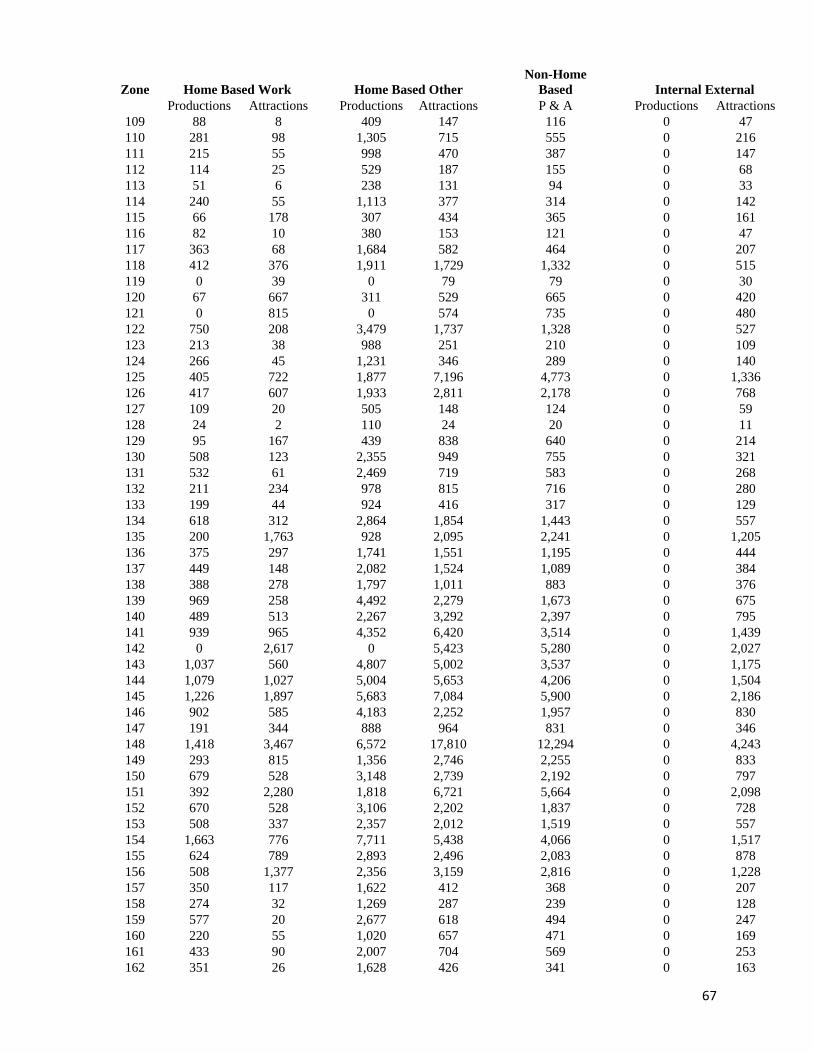
67

Zone Home Based Work Home Based Other

Non-Home

Based Internal External

Productions Attractions Productions Attractions P & A Productions Attractions

109 88 8 409 147 116 0 47

110 281 98 1,305 715 555 0 216

111 215 55 998 470 387 0 147

112 114 25 529 187 155 0 68

113 51 6 238 131 94 0 33

114 240 55 1,113 377 314 0 142

115 66 178 307 434 365 0 161

116 82 10 380 153 121 0 47

117 363 68 1,684 582 464 0 207

118 412 376 1,911 1,729 1,332 0 515

119 0 39 0 79 79 0 30

120 67 667 311 529 665 0 420

121 0 815 0 574 735 0 480

122 750 208 3,479 1,737 1,328 0 527

123 213 38 988 251 210 0 109

124 266 45 1,231 346 289 0 140

125 405 722 1,877 7,196 4,773 0 1,336

126 417 607 1,933 2,811 2,178 0 768

127 109 20 505 148 124 0 59

128 24 2 110 24 20 0 11

129 95 167 439 838 640 0 214

130 508 123 2,355 949 755 0 321

131 532 61 2,469 719 583 0 268

132 211 234 978 815 716 0 280

133 199 44 924 416 317 0 129

134 618 312 2,864 1,854 1,443 0 557

135 200 1,763 928 2,095 2,241 0 1,205

136 375 297 1,741 1,551 1,195 0 444

137 449 148 2,082 1,524 1,089 0 384

138 388 278 1,797 1,011 883 0 376

139 969 258 4,492 2,279 1,673 0 675

140 489 513 2,267 3,292 2,397 0 795

141 939 965 4,352 6,420 3,514 0 1,439

142 0 2,617 0 5,423 5,280 0 2,027

143 1,037 560 4,807 5,002 3,537 0 1,175

144 1,079 1,027 5,004 5,653 4,206 0 1,504

145 1,226 1,897 5,683 7,084 5,900 0 2,186

146 902 585 4,183 2,252 1,957 0 830

147 191 344 888 964 831 0 346

148 1,418 3,467 6,572 17,810 12,294 0 4,243

149 293 815 1,356 2,746 2,255 0 833

150 679 528 3,148 2,739 2,192 0 797

151 392 2,280 1,818 6,721 5,664 0 2,098

152 670 528 3,106 2,202 1,837 0 728

153 508 337 2,357 2,012 1,519 0 557

154 1,663 776 7,711 5,438 4,066 0 1,517

155 624 789 2,893 2,496 2,083 0 878

156 508 1,377 2,356 3,159 2,816 0 1,228

157 350 117 1,622 412 368 0 207

158 274 32 1,269 287 239 0 128

159 577 20 2,677 618 494 0 247

160 220 55 1,020 657 471 0 169

161 433 90 2,007 704 569 0 253

162 351 26 1,628 426 341 0 163

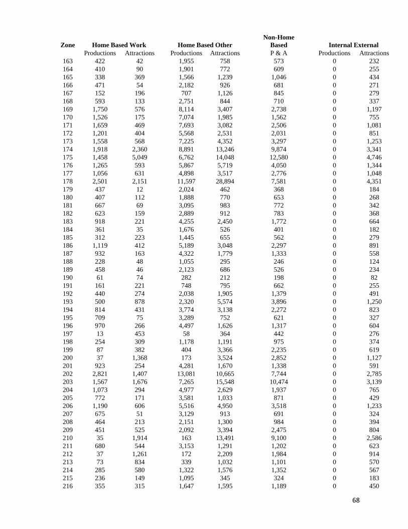
68

Zone Home Based Work Home Based Other

Non-Home

Based Internal External

Productions Attractions Productions Attractions P & A Productions Attractions

163 422 42 1,955 758 573 0 232

164 410 90 1,901 772 609 0 255

165 338 369 1,566 1,239 1,046 0 434

166 471 54 2,182 926 681 0 271

167 152 196 707 1,126 845 0 279

168 593 133 2,751 844 710 0 337

169 1,750 576 8,114 3,407 2,738 0 1,197

170 1,526 175 7,074 1,985 1,562 0 755

171 1,659 469 7,693 3,082 2,506 0 1,081

172 1,201 404 5,568 2,531 2,031 0 851

173 1,558 568 7,225 4,352 3,297 0 1,253

174 1,918 2,360 8,891 13,246 9,874 0 3,341

175 1,458 5,049 6,762 14,048 12,580 0 4,746

176 1,265 593 5,867 5,719 4,050 0 1,344

177 1,056 631 4,898 3,517 2,776 0 1,048

178 2,501 2,151 11,597 28,894 7,581 0 4,351

179 437 12 2,024 462 368 0 184

180 407 112 1,888 770 653 0 268

181 667 69 3,095 983 772 0 342

182 623 159 2,889 912 783 0 368

183 918 221 4,255 2,450 1,772 0 664

184 361 35 1,676 526 401 0 182

185 312 223 1,445 655 562 0 279

186 1,119 412 5,189 3,048 2,297 0 891

187 932 163 4,322 1,779 1,333 0 558

188 228 48 1,055 295 246 0 124

189 458 46 2,123 686 526 0 234

190 61 74 282 212 198 0 82

191 161 221 748 795 662 0 255

192 440 274 2,038 1,905 1,379 0 491

193 500 878 2,320 5,574 3,896 0 1,250

194 814 431 3,774 3,138 2,272 0 823

195 709 75 3,289 752 621 0 327

196 970 266 4,497 1,626 1,317 0 604

197 13 453 58 364 442 0 276

198 254 309 1,178 1,191 975 0 374

199 87 382 404 3,366 2,235 0 619

200 37 1,368 173 3,524 2,852 0 1,127

201 923 254 4,281 1,670 1,338 0 591

202 2,821 1,407 13,081 10,665 7,744 0 2,785

203 1,567 1,676 7,265 15,548 10,474 0 3,139

204 1,073 294 4,977 2,629 1,937 0 765

205 772 171 3,581 1,033 871 0 429

206 1,190 606 5,516 4,950 3,518 0 1,233

207 675 51 3,129 913 691 0 324

208 464 213 2,151 1,300 984 0 394

209 451 525 2,092 3,394 2,475 0 804

210 35 1,914 163 13,491 9,100 0 2,586

211 680 544 3,153 1,291 1,202 0 623

212 37 1,261 172 2,209 1,984 0 914

213 73 834 339 1,032 1,101 0 570

214 285 580 1,322 1,576 1,352 0 567

215 236 149 1,095 345 324 0 183

216 355 315 1,647 1,595 1,189 0 450

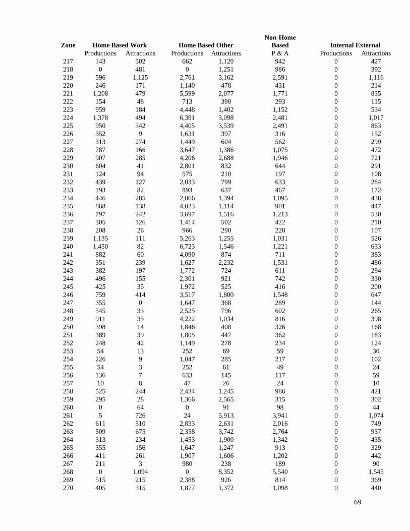
69

Zone Home Based Work Home Based Other

Non-Home

Based Internal External

Productions Attractions Productions Attractions P & A Productions Attractions

217 143 502 662 1,120 942 0 427

218 0 481 0 1,251 986 0 392

219 596 1,125 2,761 3,162 2,591 0 1,116

220 246 171 1,140 478 431 0 214

221 1,208 479 5,599 2,077 1,771 0 835

222 154 48 713 390 293 0 115

223 959 184 4,448 1,402 1,152 0 534

224 1,378 494 6,391 3,098 2,481 0 1,017

225 950 342 4,405 3,539 2,491 0 863

226 352 9 1,631 397 316 0 152

227 313 274 1,449 604 562 0 299

228 787 166 3,647 1,386 1,075 0 472

229 907 285 4,206 2,688 1,946 0 721

230 604 41 2,801 832 644 0 291

231 124 94 575 210 197 0 108

232 439 127 2,033 799 633 0 284

233 193 82 893 637 467 0 172

234 446 285 2,066 1,394 1,095 0 438

235 868 138 4,023 1,114 901 0 447

236 797 242 3,697 1,516 1,213 0 530

237 305 126 1,414 502 422 0 210

238 208 26 966 290 228 0 107

239 1,135 111 5,263 1,255 1,031 0 526

240 1,450 82 6,723 1,546 1,221 0 633

241 882 60 4,090 874 711 0 383

242 351 239 1,627 2,232 1,531 0 486

243 382 197 1,772 724 611 0 294

244 496 155 2,301 921 742 0 330

245 425 35 1,972 525 416 0 200

246 759 414 3,517 1,800 1,548 0 647

247 355 0 1,647 368 289 0 144

248 545 33 2,525 796 602 0 265

249 911 35 4,222 1,034 816 0 398

250 398 14 1,846 408 326 0 168

251 389 39 1,805 447 362 0 183

252 248 42 1,149 278 234 0 124

253 54 13 252 69 59 0 30

254 226 9 1,047 285 217 0 102

255 54 3 252 61 49 0 24

256 136 7 633 145 117 0 59

257 10 8 47 26 24 0 10

258 525 244 2,434 1,245 986 0 421

259 295 28 1,366 2,565 315 0 302

260 0 64 0 91 98 0 44

261 5 726 24 5,913 3,941 0 1,074

262 611 510 2,833 2,631 2,016 0 749

263 509 675 2,358 3,742 2,764 0 937

264 313 234 1,453 1,900 1,342 0 435

265 355 156 1,647 1,247 913 0 329

266 411 261 1,907 1,606 1,202 0 442

267 211 3 980 238 189 0 90

268 0 1,094 0 8,352 5,540 0 1,545

269 515 215 2,388 926 814 0 369

270 405 315 1,877 1,372 1,098 0 440

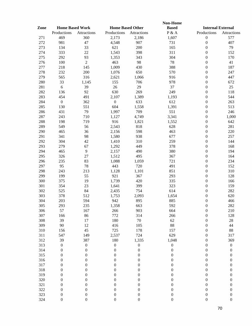
70

Zone Home Based Work Home Based Other

Non-Home

Based Internal External

Productions Attractions Productions Attractions P & A Productions Attractions

271 469 360 2,173 2,186 1,607 0 577

272 981 47 4,548 907 731 0 407

273 134 33 621 200 165 0 79

274 333 22 1,543 398 311 0 152

275 292 93 1,353 343 304 0 170

276 100 2 463 98 78 0 41

277 218 145 1,009 430 388 0 187

278 232 200 1,076 650 570 0 247

279 565 316 2,621 1,066 916 0 447

280 33 1,145 155 706 978 0 672

281 6 39 26 29 37 0 25

282 136 92 630 269 249 0 118

283 454 491 2,107 1,389 1,193 0 544

284 0 362 0 633 612 0 263

285 130 551 604 1,558 1,391 0 513

286 431 79 1,997 709 551 0 246

287 243 710 1,127 4,749 3,341 0 1,000

288 198 719 916 1,821 1,552 0 642

289 549 56 2,543 818 628 0 281

290 465 36 2,156 598 463 0 220

291 341 98 1,580 938 677 0 257

292 304 42 1,410 310 259 0 144

293 279 67 1,292 449 378 0 168

294 465 9 2,157 490 380 0 194

295 326 27 1,512 495 367 0 164

296 235 83 1,088 1,059 721 0 234

297 95 78 443 720 491 0 152

298 243 213 1,128 1,101 851 0 310

299 199 55 921 367 293 0 128

300 375 19 1,739 420 335 0 166

301 354 23 1,641 399 323 0 159

302 525 84 2,435 754 614 0 282

303 378 512 1,753 2,093 1,654 0 620

304 203 594 942 895 885 0 466

305 293 235 1,358 663 592 0 282

306 57 167 266 903 664 0 210

307 166 86 772 314 266 0 128

308 39 17 180 70 62 0 28

309 90 12 416 105 88 0 44

310 156 45 725 178 157 0 88

311 547 149 2,537 724 629 0 317

312 39 387 180 1,335 1,048 0 369

313 0 0 0 0 0 0 0

314 0 0 0 0 0 0 0

315 0 0 0 0 0 0 0

316 0 0 0 0 0 0 0

317 0 0 0 0 0 0 0

318 0 0 0 0 0 0 0

319 0 0 0 0 0 0 0

320 0 0 0 0 0 0 0

321 0 0 0 0 0 0 0

322 0 0 0 0 0 0 0

323 0 0 0 0 0 0 0

324 0 0 0 0 0 0 0

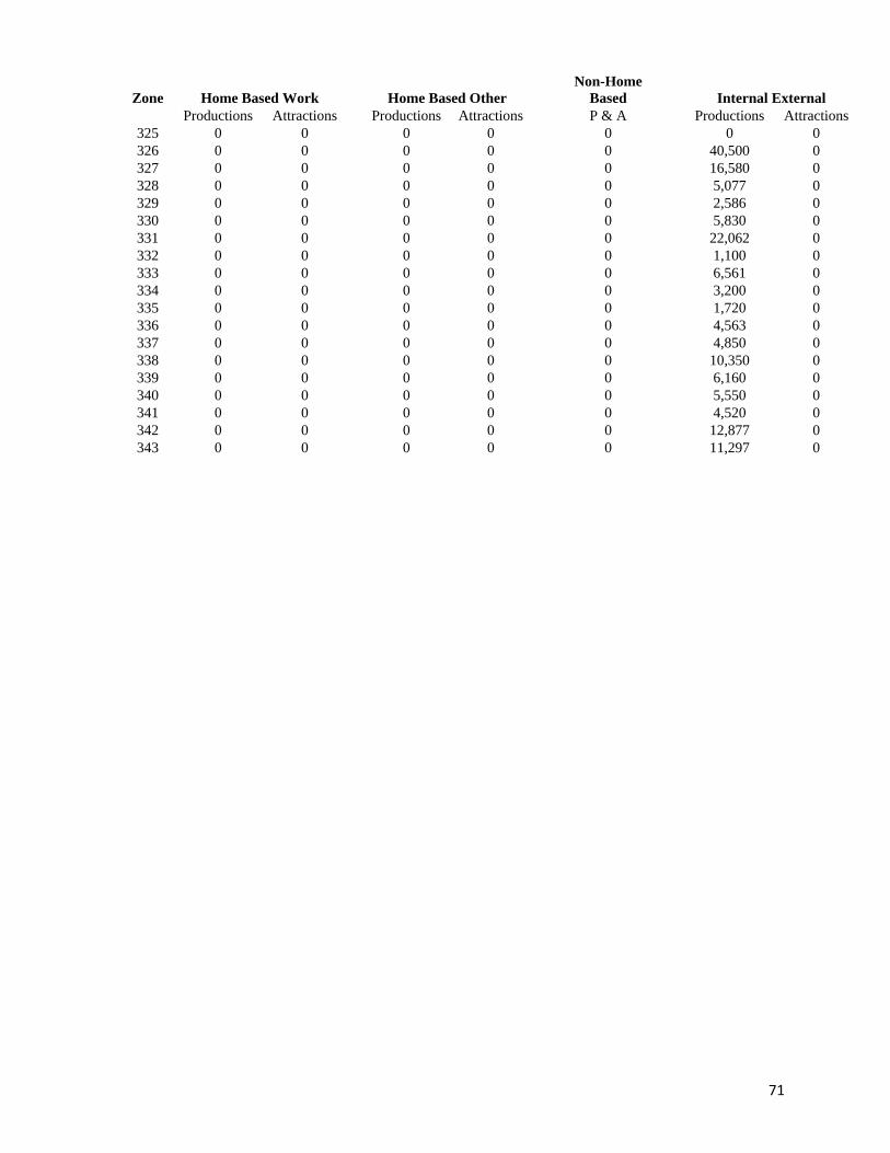
71

Zone Home Based Work Home Based Other

Non-Home

Based Internal External

Productions Attractions Productions Attractions P & A Productions Attractions

325 0 0 0 0 0 0 0

326 0 0 0 0 0 40,500 0

327 0 0 0 0 0 16,580 0

328 0 0 0 0 0 5,077 0

329 0 0 0 0 0 2,586 0

330 0 0 0 0 0 5,830 0

331 0 0 0 0 0 22,062 0

332 0 0 0 0 0 1,100 0

333 0 0 0 0 0 6,561 0

334 0 0 0 0 0 3,200 0

335 0 0 0 0 0 1,720 0

336 0 0 0 0 0 4,563 0

337 0 0 0 0 0 4,850 0

338 0 0 0 0 0 10,350 0

339 0 0 0 0 0 6,160 0

340 0 0 0 0 0 5,550 0

341 0 0 0 0 0 4,520 0

342 0 0 0 0 0 12,877 0

343 0 0 0 0 0 11,297 0

72

Appendix A5 2045 Trip Ends

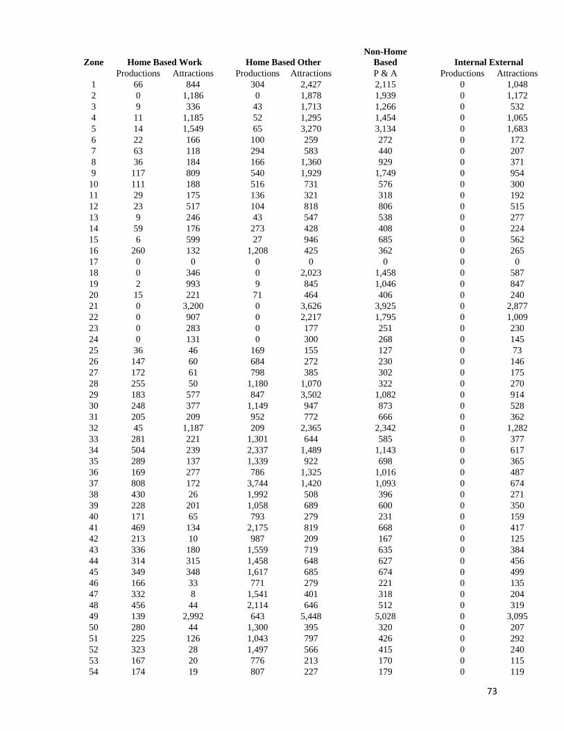
73

Zone Home Based Work Home Based Other

Non-Home

Based Internal External

Productions Attractions Productions Attractions P & A Productions Attractions

1 66 844 304 2,427 2,115 0 1,048

2 0 1,186 0 1,878 1,939 0 1,172

3 9 336 43 1,713 1,266 0 532

4 11 1,185 52 1,295 1,454 0 1,065

5 14 1,549 65 3,270 3,134 0 1,683

6 22 166 100 259 272 0 172

7 63 118 294 583 440 0 207

8 36 184 166 1,360 929 0 371

9 117 809 540 1,929 1,749 0 954

10 111 188 516 731 576 0 300

11 29 175 136 321 318 0 192

12 23 517 104 818 806 0 515

13 9 246 43 547 538 0 277

14 59 176 273 428 408 0 224

15 6 599 27 946 685 0 562

16 260 132 1,208 425 362 0 265

17 0 0 0 0 0 0 0

18 0 346 0 2,023 1,458 0 587

19 2 993 9 845 1,046 0 847

20 15 221 71 464 406 0 240

21 0 3,200 0 3,626 3,925 0 2,877

22 0 907 0 2,217 1,795 0 1,009

23 0 283 0 177 251 0 230

24 0 131 0 300 268 0 145

25 36 46 169 155 127 0 73

26 147 60 684 272 230 0 146

27 172 61 798 385 302 0 175

28 255 50 1,180 1,070 322 0 270

29 183 577 847 3,502 1,082 0 914

30 248 377 1,149 947 873 0 528

31 205 209 952 772 666 0 362

32 45 1,187 209 2,365 2,342 0 1,282

33 281 221 1,301 644 585 0 377

34 504 239 2,337 1,489 1,143 0 617

35 289 137 1,339 922 698 0 365

36 169 277 786 1,325 1,016 0 487

37 808 172 3,744 1,420 1,093 0 674

38 430 26 1,992 508 396 0 271

39 228 201 1,058 689 600 0 350

40 171 65 793 279 231 0 159

41 469 134 2,175 819 668 0 417

42 213 10 987 209 167 0 125

43 336 180 1,559 719 635 0 384

44 314 315 1,458 648 627 0 456

45 349 348 1,617 685 674 0 499

46 166 33 771 279 221 0 135

47 332 8 1,541 401 318 0 204

48 456 44 2,114 646 512 0 319

49 139 2,992 643 5,448 5,028 0 3,095

50 280 44 1,300 395 320 0 207

51 225 126 1,043 797 426 0 292

52 323 28 1,497 566 415 0 240

53 167 20 776 213 170 0 115

54 174 19 807 227 179 0 119

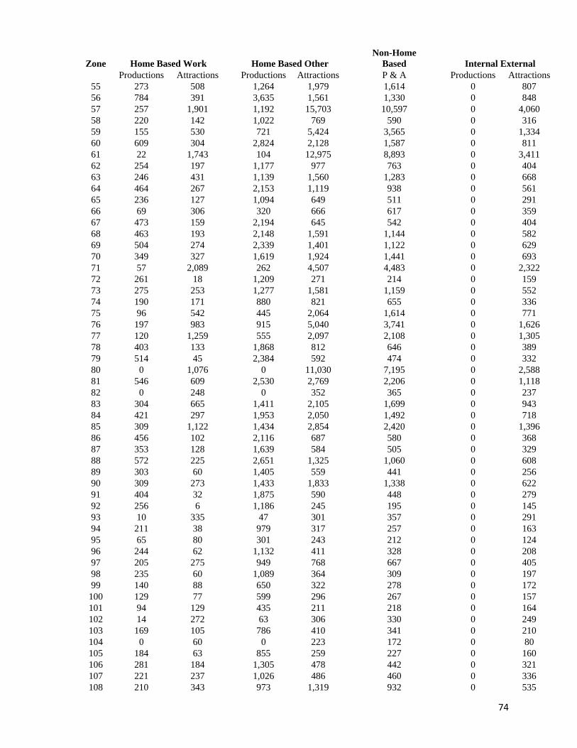
74

Zone Home Based Work Home Based Other

Non-Home

Based Internal External

Productions Attractions Productions Attractions P & A Productions Attractions

55 273 508 1,264 1,979 1,614 0 807

56 784 391 3,635 1,561 1,330 0 848

57 257 1,901 1,192 15,703 10,597 0 4,060

58 220 142 1,022 769 590 0 316

59 155 530 721 5,424 3,565 0 1,334

60 609 304 2,824 2,128 1,587 0 811

61 22 1,743 104 12,975 8,893 0 3,411

62 254 197 1,177 977 763 0 404

63 246 431 1,139 1,560 1,283 0 668

64 464 267 2,153 1,119 938 0 561

65 236 127 1,094 649 511 0 291

66 69 306 320 666 617 0 359

67 473 159 2,194 645 542 0 404

68 463 193 2,148 1,591 1,144 0 582

69 504 274 2,339 1,401 1,122 0 629

70 349 327 1,619 1,924 1,441 0 693

71 57 2,089 262 4,507 4,483 0 2,322

72 261 18 1,209 271 214 0 159

73 275 253 1,277 1,581 1,159 0 552

74 190 171 880 821 655 0 336

75 96 542 445 2,064 1,614 0 771

76 197 983 915 5,040 3,741 0 1,626

77 120 1,259 555 2,097 2,108 0 1,305

78 403 133 1,868 812 646 0 389

79 514 45 2,384 592 474 0 332

80 0 1,076 0 11,030 7,195 0 2,588

81 546 609 2,530 2,769 2,206 0 1,118

82 0 248 0 352 365 0 237

83 304 665 1,411 2,105 1,699 0 943

84 421 297 1,953 2,050 1,492 0 718

85 309 1,122 1,434 2,854 2,420 0 1,396

86 456 102 2,116 687 580 0 368

87 353 128 1,639 584 505 0 329

88 572 225 2,651 1,325 1,060 0 608

89 303 60 1,405 559 441 0 256

90 309 273 1,433 1,833 1,338 0 622

91 404 32 1,875 590 448 0 279

92 256 6 1,186 245 195 0 145

93 10 335 47 301 357 0 291

94 211 38 979 317 257 0 163

95 65 80 301 243 212 0 124

96 244 62 1,132 411 328 0 208

97 205 275 949 768 667 0 405

98 235 60 1,089 364 309 0 197

99 140 88 650 322 278 0 172

100 129 77 599 296 267 0 157

101 94 129 435 211 218 0 164

102 14 272 63 306 330 0 249

103 169 105 786 410 341 0 210

104 0 60 0 223 172 0 80

105 184 63 855 259 227 0 160

106 281 184 1,305 478 442 0 321

107 221 237 1,026 486 460 0 336

108 210 343 973 1,319 932 0 535

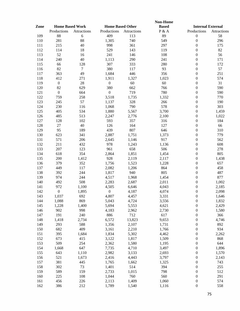
75

Zone Home Based Work Home Based Other

Non-Home

Based Internal External

Productions Attractions Productions Attractions P & A Productions Attractions

109 88 6 409 113 89 0 58

110 281 88 1,305 740 549 0 296

111 215 40 998 361 297 0 175

112 114 18 529 143 119 0 82

113 52 16 241 146 108 0 56

114 240 40 1,113 290 241 0 171

115 66 128 307 333 280 0 172

116 82 7 380 117 93 0 57

117 363 49 1,684 446 356 0 251

118 412 271 1,911 1,327 1,023 0 574

119 0 28 0 60 60 0 31

120 82 629 380 662 766 0 590

121 0 664 0 719 780 0 590

122 759 258 3,518 1,735 1,332 0 770

123 245 57 1,137 328 266 0 190

124 230 116 1,068 790 578 0 303

125 405 534 1,880 5,567 3,700 0 1,459

126 485 513 2,247 2,776 2,100 0 1,022

127 128 102 593 357 316 0 184

128 27 40 126 164 127 0 66

129 95 189 439 807 646 0 310

130 623 341 2,887 1,751 1,373 0 779

131 571 206 2,645 1,146 917 0 562

132 211 432 978 1,243 1,136 0 608

133 207 123 961 658 506 0 278

134 618 354 2,864 1,851 1,454 0 805

135 200 1,412 928 2,119 2,117 0 1,438

136 379 352 1,756 1,523 1,228 0 657

137 449 117 2,082 1,206 864 0 458

138 392 244 1,817 940 805 0 487

139 974 244 4,517 1,968 1,454 0 877

140 492 508 2,283 2,687 2,011 0 1,002

141 972 1,100 4,505 6,646 4,043 0 2,185

142 0 1,895 0 4,187 4,074 0 2,098

143 1,037 692 4,807 4,457 3,331 0 1,646

144 1,088 869 5,043 4,724 3,556 0 1,832

145 1,228 1,400 5,694 5,553 4,621 0 2,429

146 902 998 4,183 2,962 2,730 0 1,580

147 191 240 886 712 617 0 366

148 1,418 2,734 6,572 13,823 9,653 0 4,746

149 293 588 1,356 2,107 1,731 0 892

150 682 409 3,161 2,210 1,766 0 934

151 395 1,684 1,834 5,302 4,462 0 2,262

152 673 415 3,122 1,817 1,509 0 868

153 509 254 2,362 1,580 1,195 0 644

154 1,668 647 7,735 4,710 3,497 0 1,896

155 643 1,110 2,982 3,133 2,693 0 1,570

156 521 1,673 2,416 4,443 3,797 0 2,143

157 381 445 1,765 1,662 1,325 0 743

158 302 73 1,401 514 394 0 255

159 589 159 2,733 1,015 798 0 512

160 225 108 1,044 760 560 0 291

161 456 226 2,113 1,409 1,060 0 574

162 386 212 1,789 1,540 1,116 0 558

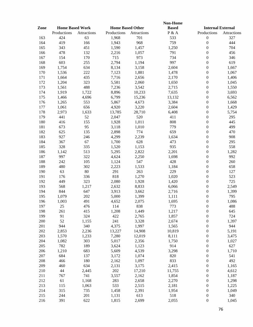
76

Zone Home Based Work Home Based Other

Non-Home

Based Internal External

Productions Attractions Productions Attractions P & A Productions Attractions

163 424 63 1,968 701 533 0 327

164 419 166 1,943 968 759 0 444

165 343 451 1,590 1,457 1,250 0 704

166 478 132 2,216 1,057 791 0 456

167 154 170 715 973 734 0 346

168 603 255 2,794 1,194 997 0 619

169 1,754 634 8,134 3,158 2,604 0 1,667

170 1,536 222 7,123 1,881 1,478 0 1,067

171 1,664 435 7,716 2,656 2,170 0 1,406

172 1,204 323 5,581 2,060 1,650 0 1,045

173 1,561 488 7,236 3,542 2,715 0 1,550

174 1,919 1,722 8,896 10,233 7,635 0 3,693

175 1,466 4,696 6,799 15,236 13,132 0 6,562

176 1,265 553 5,867 4,673 3,384 0 1,668

177 1,061 656 4,920 3,220 2,604 0 1,429

178 2,973 1,633 13,785 28,710 6,408 0 5,754

179 441 52 2,047 520 411 0 295

180 416 155 1,928 1,011 808 0 445

181 673 95 3,118 1,010 779 0 499

182 625 135 2,898 774 659 0 470

183 927 246 4,299 2,239 1,634 0 908

184 367 67 1,700 628 473 0 295

185 328 335 1,520 1,153 935 0 558

186 1,142 513 5,295 2,822 2,201 0 1,282

187 997 322 4,624 2,250 1,698 0 992

188 242 105 1,124 547 428 0 260

189 480 302 2,223 1,533 1,184 0 658

190 63 80 291 263 229 0 127

191 176 336 818 1,270 1,020 0 523

192 449 323 2,080 1,928 1,420 0 725

193 568 1,217 2,632 8,833 6,066 0 2,549

194 844 647 3,913 3,662 2,716 0 1,399

195 1,079 202 5,000 1,399 1,111 0 795

196 1,003 491 4,652 2,075 1,695 0 1,086

197 25 476 114 838 773 0 488

198 261 415 1,208 1,449 1,217 0 645

199 91 324 422 2,765 1,857 0 724

200 52 1,155 241 3,328 2,674 0 1,397

201 944 340 4,375 1,997 1,565 0 944

202 2,853 2,236 13,227 14,908 10,819 0 5,191

203 1,570 1,233 7,280 12,019 8,111 0 3,475

204 1,082 303 5,017 2,356 1,750 0 1,027

205 782 189 3,624 1,123 914 0 627

206 1,210 683 5,609 4,539 3,298 0 1,710

207 684 137 3,172 1,074 820 0 541

208 466 180 2,162 1,097 833 0 492

209 460 634 2,131 3,175 2,415 0 1,165

210 44 2,445 202 17,210 11,755 0 4,612

211 767 741 3,557 2,162 1,854 0 1,187

212 61 1,168 283 2,658 2,270 0 1,298

213 115 1,063 533 2,515 2,181 0 1,225

214 315 735 1,458 2,391 1,954 0 1,049

215 244 201 1,131 613 518 0 340

216 391 622 1,815 2,699 2,055 0 1,045

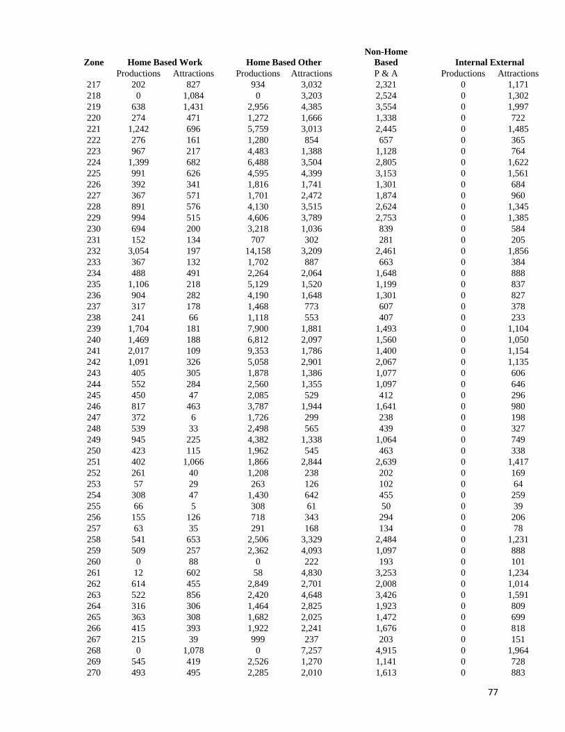
77

Zone Home Based Work Home Based Other

Non-Home

Based Internal External

Productions Attractions Productions Attractions P & A Productions Attractions

217 202 827 934 3,032 2,321 0 1,171

218 0 1,084 0 3,203 2,524 0 1,302

219 638 1,431 2,956 4,385 3,554 0 1,997

220 274 471 1,272 1,666 1,338 0 722

221 1,242 696 5,759 3,013 2,445 0 1,485

222 276 161 1,280 854 657 0 365

223 967 217 4,483 1,388 1,128 0 764

224 1,399 682 6,488 3,504 2,805 0 1,622

225 991 626 4,595 4,399 3,153 0 1,561

226 392 341 1,816 1,741 1,301 0 684

227 367 571 1,701 2,472 1,874 0 960

228 891 576 4,130 3,515 2,624 0 1,345

229 994 515 4,606 3,789 2,753 0 1,385

230 694 200 3,218 1,036 839 0 584

231 152 134 707 302 281 0 205

232 3,054 197 14,158 3,209 2,461 0 1,856

233 367 132 1,702 887 663 0 384

234 488 491 2,264 2,064 1,648 0 888

235 1,106 218 5,129 1,520 1,199 0 837

236 904 282 4,190 1,648 1,301 0 827

237 317 178 1,468 773 607 0 378

238 241 66 1,118 553 407 0 233

239 1,704 181 7,900 1,881 1,493 0 1,104

240 1,469 188 6,812 2,097 1,560 0 1,050

241 2,017 109 9,353 1,786 1,400 0 1,154

242 1,091 326 5,058 2,901 2,067 0 1,135

243 405 305 1,878 1,386 1,077 0 606

244 552 284 2,560 1,355 1,097 0 646

245 450 47 2,085 529 412 0 296

246 817 463 3,787 1,944 1,641 0 980

247 372 6 1,726 299 238 0 198

248 539 33 2,498 565 439 0 327

249 945 225 4,382 1,338 1,064 0 749

250 423 115 1,962 545 463 0 338

251 402 1,066 1,866 2,844 2,639 0 1,417

252 261 40 1,208 238 202 0 169

253 57 29 263 126 102 0 64

254 308 47 1,430 642 455 0 259

255 66 5 308 61 50 0 39

256 155 126 718 343 294 0 206

257 63 35 291 168 134 0 78

258 541 653 2,506 3,329 2,484 0 1,231

259 509 257 2,362 4,093 1,097 0 888

260 0 88 0 222 193 0 101

261 12 602 58 4,830 3,253 0 1,234

262 614 455 2,849 2,701 2,008 0 1,014

263 522 856 2,420 4,648 3,426 0 1,591

264 316 306 1,464 2,825 1,923 0 809

265 363 308 1,682 2,025 1,472 0 699

266 415 393 1,922 2,241 1,676 0 818

267 215 39 999 237 203 0 151

268 0 1,078 0 7,257 4,915 0 1,964

269 545 419 2,526 1,270 1,141 0 728

270 493 495 2,285 2,010 1,613 0 883

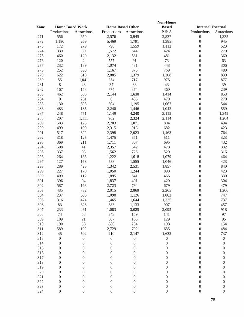
78

Zone Home Based Work Home Based Other

Non-Home

Based Internal External

Productions Attractions Productions Attractions P & A Productions Attractions

271 556 650 2,576 3,945 2,837 0 1,335

272 1,180 269 5,469 1,791 1,385 0 945

273 172 279 798 1,559 1,112 0 523

274 339 80 1,572 544 424 0 279

275 460 120 2,132 581 481 0 360

276 120 2 557 91 73 0 63

277 232 189 1,074 481 443 0 306

278 252 330 1,167 875 769 0 480

279 622 518 2,885 1,379 1,208 0 839

280 55 1,041 254 717 975 0 877

281 8 43 37 33 43 0 39

282 167 153 774 374 360 0 239

283 462 556 2,144 1,638 1,414 0 853

284 0 261 0 485 470 0 270

285 130 398 604 1,195 1,067 0 544

286 483 185 2,240 1,446 1,042 0 559

287 248 751 1,149 4,240 3,115 0 1,345

288 207 1,111 962 2,324 2,114 0 1,264

289 583 125 2,703 1,071 804 0 494

290 499 109 2,315 916 682 0 423

291 517 322 2,398 2,023 1,463 0 764

292 318 125 1,475 671 511 0 323

293 369 211 1,711 807 695 0 432

294 508 41 2,357 642 478 0 332

295 337 93 1,562 726 529 0 316

296 264 133 1,222 1,618 1,079 0 464

297 127 163 588 1,555 1,046 0 423

298 289 425 1,342 2,531 1,857 0 840

299 227 178 1,050 1,244 898 0 423

300 409 112 1,895 541 465 0 330

301 396 94 1,837 491 420 0 304

302 587 163 2,723 794 679 0 479

303 435 782 2,015 2,869 2,265 0 1,206

304 237 656 1,098 1,126 1,082 0 747

305 316 474 1,465 1,644 1,335 0 737

306 83 328 383 1,133 907 0 457

307 233 461 1,083 3,025 2,095 0 918

308 74 58 343 159 141 0 97

309 109 21 507 165 129 0 85

310 190 58 880 234 198 0 154

311 589 192 2,729 702 635 0 484

312 45 502 210 2,147 1,632 0 737

313 0 0 0 0 0 0 0

314 0 0 0 0 0 0 0

315 0 0 0 0 0 0 0

316 0 0 0 0 0 0 0

317 0 0 0 0 0 0 0

318 0 0 0 0 0 0 0

319 0 0 0 0 0 0 0

320 0 0 0 0 0 0 0

321 0 0 0 0 0 0 0

322 0 0 0 0 0 0 0

323 0 0 0 0 0 0 0

324 0 0 0 0 0 0 0

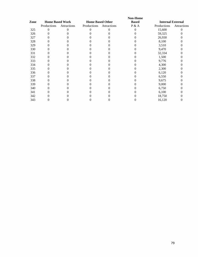
79

Zone Home Based Work Home Based Other

Non-Home

Based Internal External

Productions Attractions Productions Attractions P & A Productions Attractions

325 0 0 0 0 0 15,600 0

326 0 0 0 0 0 59,325 0

327 0 0 0 0 0 26,930 0

328 0 0 0 0 0 8,100 0

329 0 0 0 0 0 3,510 0

330 0 0 0 0 0 9,470 0

331 0 0 0 0 0 32,334 0

332 0 0 0 0 0 1,500 0

333 0 0 0 0 0 9,776 0

334 0 0 0 0 0 4,300 0

335 0 0 0 0 0 2,300 0

336 0 0 0 0 0 6,120 0

337 0 0 0 0 0 6,550 0

338 0 0 0 0 0 9,675 0

339 0 0 0 0 0 9,000 0

340 0 0 0 0 0 6,750 0

341 0 0 0 0 0 6,100 0

342 0 0 0 0 0 18,750 0

343 0 0 0 0 0 16,120 0

80

Appendix A6 MATS Link Codes, Capacities, and Coded

Speeds

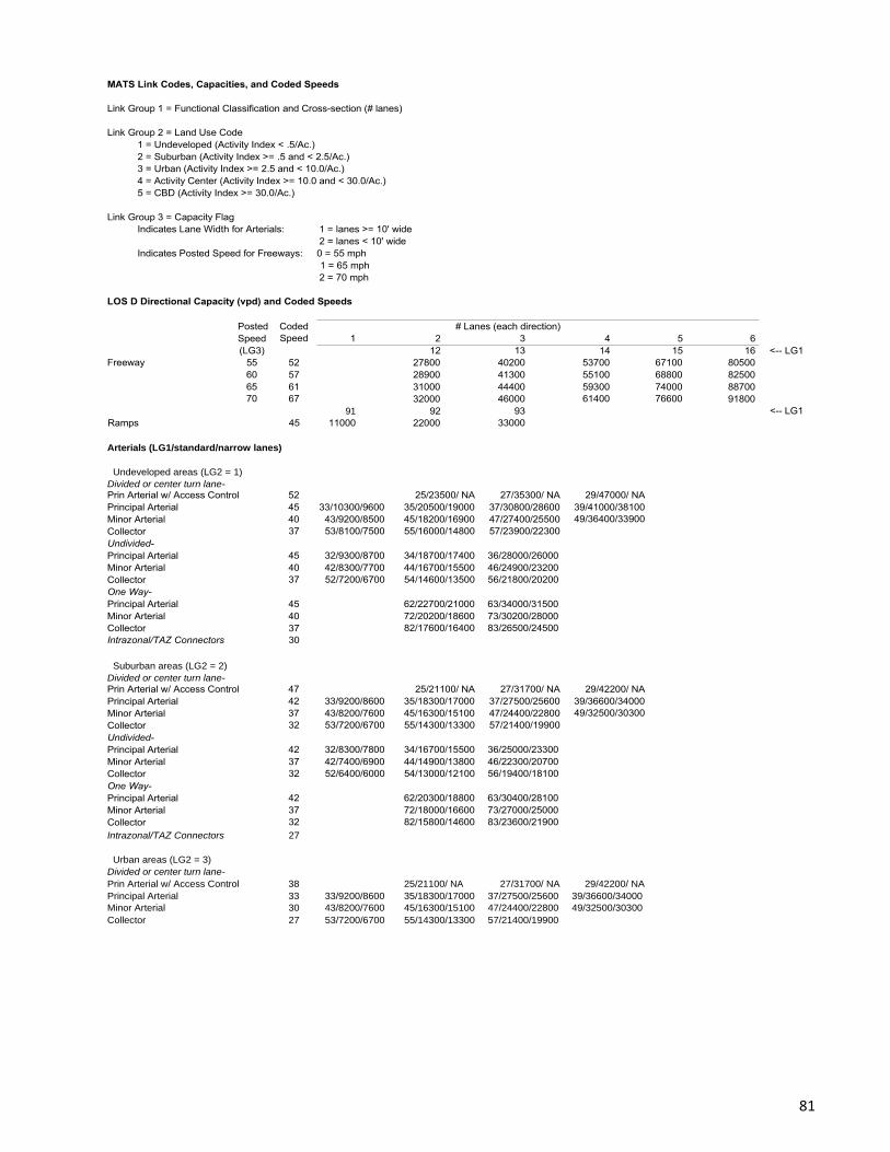
81

Arterials (LG1/standard/narrow lanes)

Undeveloped areas (LG2 = 1)

Divided or center turn lane-

Suburban areas (LG2 = 2)

Divided or center turn lane-

Intrazonal/TAZ Connectors 27

Urban areas (LG2 = 3)

Divided or center turn lane-

Prin Arterial w/ Access Control 38 25/21100/ NA 27/31700/ NA 29/42200/ NA

Principal Arterial 33 33/9200/8600 35/18300/17000 37/27500/25600 39/36600/34000

Minor Arterial 30 43/8200/7600 45/16300/15100 47/24400/22800 49/32500/30300

Collector 27 53/7200/6700 55/14300/13300 57/21400/19900

91

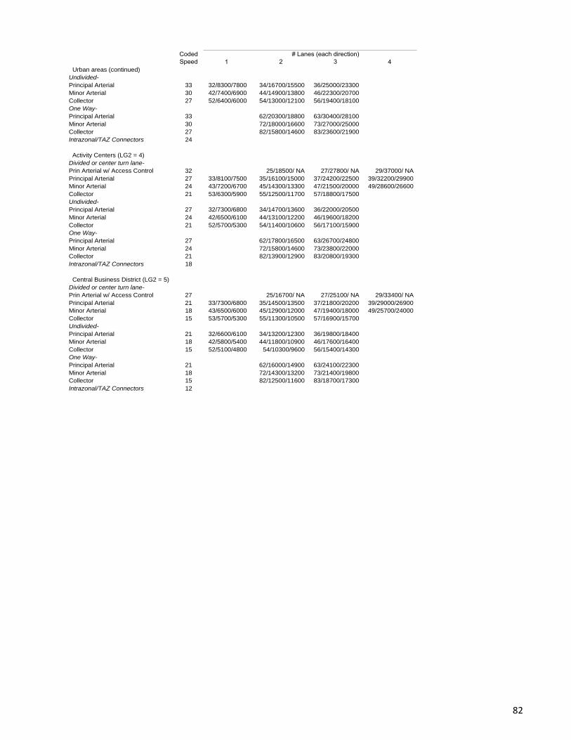
82

Urban areas (continued)

Undivided-

Principal Arterial

33

32/8300/7800

34/16700/15500

36/25000/23300

Minor Arterial 30 42/7400/6900 44/14900/13800 46/22300/20700

Collector

One Way-

Principal Arterial

27

33

52/6400/6000 54/13000/12100

62/20300/18800

56/19400/18100

63/30400/28100

Minor Arterial 30 72/18000/16600 73/27000/25000

Collector 27 82/15800/14600 83/23600/21900

Intrazonal/TAZ Connectors 24 Activity Centers (LG2 = 4)

Divided or center turn lane-

Prin Arterial w/ Access Control

32

25/18500/ NA

27/27800/ NA

29/37000/ NA

Principal Arterial 27 33/8100/7500 35/16100/15000 37/24200/22500 39/32200/29900

Minor Arterial 24 43/7200/6700 45/14300/13300 47/21500/20000 49/28600/26600

Collector

Undivided-

Principal Arterial

21

27

53/6300/5900

32/7300/6800

55/12500/11700

34/14700/13600

57/18800/17500

36/22000/20500

Minor Arterial 24 42/6500/6100 44/13100/12200 46/19600/18200 Collector

One Way-

Principal Arterial

21

27

52/5700/5300 54/11400/10600

62/17800/16500

56/17100/15900

63/26700/24800

Minor Arterial 24 72/15800/14600 73/23800/22000 Collector 21 82/13900/12900 83/20800/19300 Intrazonal/TAZ Connectors 18

Central Business District (LG2 = 5)

Divided or center turn lane-

Prin Arterial w/ Access Control

27

25/16700/ NA

27/25100/ NA

29/33400/ NA

Principal Arterial 21 33/7300/6800 35/14500/13500 37/21800/20200 39/29000/26900

Minor Arterial 18 43/6500/6000 45/12900/12000 47/19400/18000 49/25700/24000

Collector

Undivided-

Principal Arterial

15

21

53/5700/5300

32/6600/6100

55/11300/10500

34/13200/12300

57/16900/15700

36/19800/18400

Minor Arterial 18 42/5800/5400 44/11800/10900 46/17600/16400 Collector

One Way-

Principal Arterial

15

21

52/5100/4800 54/10300/9600

62/16000/14900

56/15400/14300

63/24100/22300

Minor Arterial 18 72/14300/13200 73/21400/19800 Collector 15 82/12500/11600 83/18700/17300 Intrazonal/TAZ Connectors 12

83

Appendix A7 Friction Factors

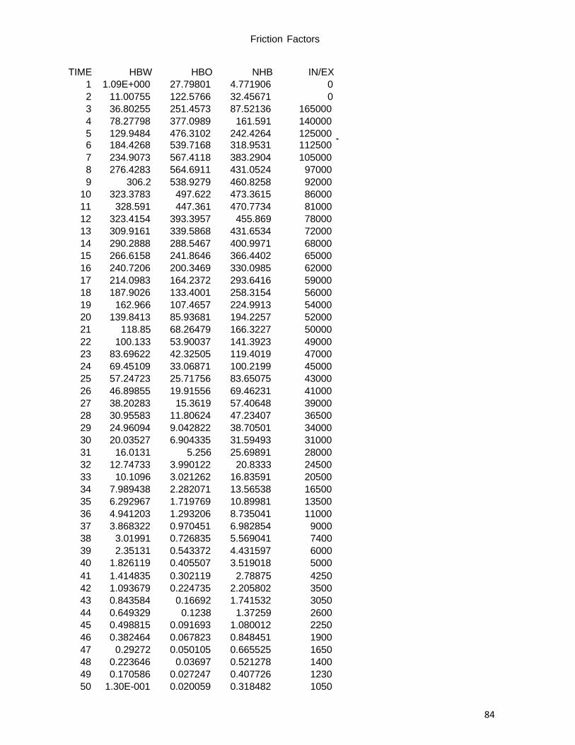
84

Friction Factors

TIME

1

HBW

1.09E+000

HBO

27.79801

NHB

4.771906

IN/EX

0

2 11.00755 122.5766 32.45671 0

3 36.80255 251.4573 87.52136 165000

4 78.27798 377.0989 161.591 140000

5 129.9484 476.3102 242.4264 125000 6 184.4268 539.7168 318.9531 112500

7 234.9073 567.4118 383.2904 105000

8 276.4283 564.6911 431.0524 97000

9 306.2 538.9279 460.8258 92000

10 323.3783 497.622 473.3615 86000

11 328.591 447.361 470.7734 81000

12 323.4154 393.3957 455.869 78000

13 309.9161 339.5868 431.6534 72000

14 290.2888 288.5467 400.9971 68000

15 266.6158 241.8646 366.4402 65000

16 240.7206 200.3469 330.0985 62000

17 214.0983 164.2372 293.6416 59000

18 187.9026 133.4001 258.3154 56000

19 162.966 107.4657 224.9913 54000

20 139.8413 85.93681 194.2257 52000

21 118.85 68.26479 166.3227 50000

22 100.133 53.90037 141.3923 49000

23 83.69622 42.32505 119.4019 47000

24 69.45109 33.06871 100.2199 45000

25 57.24723 25.71756 83.65075 43000

26 46.89855 19.91556 69.46231 41000

27 38.20283 15.3619 57.40648 39000

28 30.95583 11.80624 47.23407 36500

29 24.96094 9.042822 38.70501 34000

30 20.03527 6.904335 31.59493 31000

31 16.0131 5.256 25.69891 28000

32 12.74733 3.990122 20.8333 24500

33 10.1096 3.021262 16.83591 20500

34 7.989438 2.282071 13.56538 16500

35 6.292967 1.719769 10.89981 13500

36 4.941203 1.293206 8.735041 11000

37 3.868322 0.970451 6.982854 9000

38 3.01991 0.726835 5.569041 7400

39 2.35131 0.543372 4.431597 6000

40 1.826119 0.405507 3.519018 5000

41 1.414835 0.302119 2.78875 4250

42 1.093679 0.224735 2.205802 3500

43 0.843584 0.16692 1.741532 3050

44 0.649329 0.1238 1.37259 2600

45 0.498815 0.091693 1.080012 2250

46 0.382464 0.067823 0.848451 1900

47 0.29272 0.050105 0.665525 1650

48 0.223646 0.03697 0.521278 1400

49 0.170586 0.027247 0.407726 1230

50 1.30E-001 0.020059 0.318482 1050

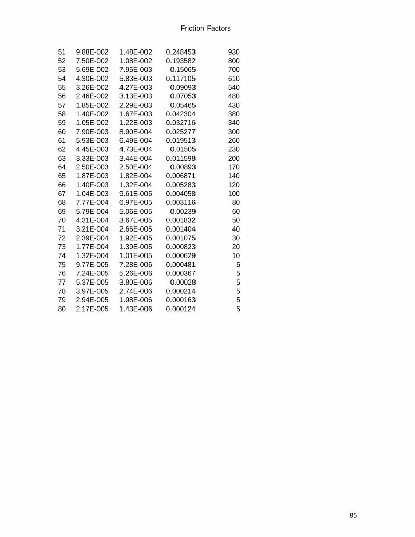
85

Friction Factors

51 9.88E-002 1.48E-002 0.248453 930

52 7.50E-002 1.08E-002 0.193582 800

53 5.69E-002 7.95E-003 0.15065 700

54 4.30E-002 5.83E-003 0.117105 610

55 3.26E-002 4.27E-003 0.09093 540

56 2.46E-002 3.13E-003 0.07053 480

57 1.85E-002 2.29E-003 0.05465 430

58 1.40E-002 1.67E-003 0.042304 380

59 1.05E-002 1.22E-003 0.032716 340

60 7.90E-003 8.90E-004 0.025277 300

61 5.93E-003 6.49E-004 0.019513 260

62 4.45E-003 4.73E-004 0.01505 230

63 3.33E-003 3.44E-004 0.011598 200

64 2.50E-003 2.50E-004 0.00893 170

65 1.87E-003 1.82E-004 0.006871 140

66 1.40E-003 1.32E-004 0.005283 120

67 1.04E-003 9.61E-005 0.004058 100

68 7.77E-004 6.97E-005 0.003116 80

69 5.79E-004 5.06E-005 0.00239 60

70 4.31E-004 3.67E-005 0.001832 50

71 3.21E-004 2.66E-005 0.001404 40

72 2.39E-004 1.92E-005 0.001075 30

73 1.77E-004 1.39E-005 0.000823 20

74 1.32E-004 1.01E-005 0.000629 10

75 9.77E-005 7.28E-006 0.000481 5

76 7.24E-005 5.26E-006 0.000367 5

77 5.37E-005 3.80E-006 0.00028 5

78 3.97E-005 2.74E-006 0.000214 5

79 2.94E-005 1.98E-006 0.000163 5

80 2.17E-005 1.43E-006 0.000124 5

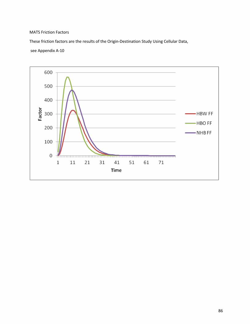
86

MATS Friction Factors

These friction factors are the results of the Origin-Destination Study Using Cellular Data,

see Appendix A-10

87

Appendix A8 Screenline Error

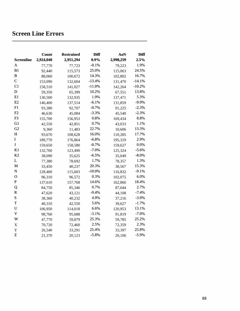
88

Screen Line Errors

Count Restrained Diff AoN Diff

Screenline 2,924,040 2,951,294 0.9% 2,998,259 2.5%

A 77,770 77,723 -0.1% 79,223 1.9%

B1 92,440 115,573 25.0% 115,063 24.5%

B 88,060 100,672 14.3% 102,802 16.7%

C 153,090 132,604 -13.4% 131,470 -14.1%

C1 158,510 141,027 -11.0% 142,264 -10.2%

D 59,350 65,399 10.2% 67,551 13.8%

E1 130,500 132,935 1.9% 137,471 5.3%

E2 146,400 137,514 -6.1% 131,859 -9.9%

F1 93,380 92,707 -0.7% 91,225 -2.3%

F2 46,630 45,084 -3.3% 45,540 -2.3%

F3 155,700 156,953 0.8% 169,434 8.8%

G1 42,550 42,851 0.7% 43,033 1.1%

G2 9,360 11,483 22.7% 10,606 13.3%

H 93,670 108,628 16.0% 110,285 17.7%

I 189,770 176,864 -6.8% 195,319 2.9%

J 159,650 158,580 -0.7% 159,627 0.0%

K1 132,760 123,490 -7.0% 125,324 -5.6%

K2 38,090 35,625 -6.5% 35,049 -8.0%

L 77,380 78,692 1.7% 78,357 1.3%

M 33,450 40,237 20.3% 38,567 15.3%

N 128,460 115,603 -10.0% 116,832 -9.1%

O 96,310 96,572 0.3% 102,075 6.0%

P 137,610 157,768 14.6% 162,866 18.4%

Q 84,750 85,346 0.7% 87,044 2.7%

R 47,620 43,121 -9.4% 44,108 -7.4%

S 38,360 40,232 4.9% 37,216 -3.0%

T 40,310 42,550 5.6% 39,627 -1.7%

U 106,950 114,018 6.6% 120,953 13.1%

V 98,760 95,688 -3.1% 91,819 -7.0%

W 47,770 59,879 25.3% 59,785 25.2%

X 70,720 72,460 2.5% 72,359 2.3%

Y 26,540 33,291 25.4% 33,397 25.8%

Z 21,370 20,123 -5.8% 20,106 -5.9%

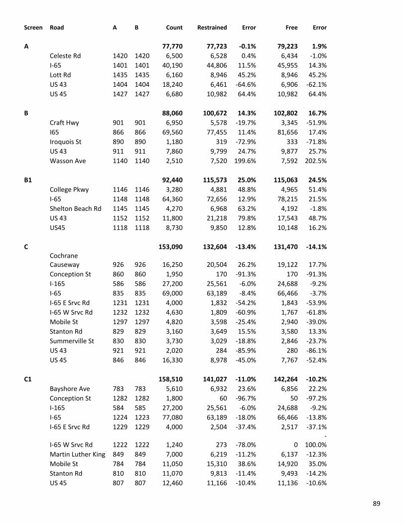
89

Screen Road A B Count Restrained Error Free Error

A 77,770 77,723 -0.1% 79,223 1.9%

Celeste Rd 1420 1420 6,500 6,528 0.4% 6,434 -1.0%

I-65 1401 1401 40,190 44,806 11.5% 45,955 14.3%

Lott Rd 1435 1435 6,160 8,946 45.2% 8,946 45.2%

US 43 1404 1404 18,240 6,461 -64.6% 6,906 -62.1%

US 45 1427 1427 6,680 10,982 64.4% 10,982 64.4%

B 88,060 100,672 14.3% 102,802 16.7%

Craft Hwy 901 901 6,950 5,578 -19.7% 3,345 -51.9%

I65 866 866 69,560 77,455 11.4% 81,656 17.4%

Iroquois St 890 890 1,180 319 -72.9% 333 -71.8%

US 43 911 911 7,860 9,799 24.7% 9,877 25.7%

Wasson Ave 1140 1140 2,510 7,520 199.6% 7,592 202.5%

B1 92,440 115,573 25.0% 115,063 24.5%

College Pkwy 1146 1146 3,280 4,881 48.8% 4,965 51.4%

I-65 1148 1148 64,360 72,656 12.9% 78,215 21.5%

Shelton Beach Rd 1145 1145 4,270 6,968 63.2% 4,192 -1.8%

US 43 1152 1152 11,800 21,218 79.8% 17,543 48.7%

US45 1118 1118 8,730 9,850 12.8% 10,148 16.2%

C 153,090 132,604 -13.4% 131,470 -14.1%

Cochrane Causeway 926 926 16,250 20,504 26.2% 19,122 17.7%

Conception St 860 860 1,950 170 -91.3% 170 -91.3%

I-165 586 586 27,200 25,561 -6.0% 24,688 -9.2%

I-65 835 835 69,000 63,189 -8.4% 66,466 -3.7%

I-65 E Srvc Rd 1231 1231 4,000 1,832 -54.2% 1,843 -53.9%

I-65 W Srvc Rd 1232 1232 4,630 1,809 -60.9% 1,767 -61.8%

Mobile St 1297 1297 4,820 3,598 -25.4% 2,940 -39.0%

Stanton Rd 829 829 3,160 3,649 15.5% 3,580 13.3%

Summerville St 830 830 3,730 3,029 -18.8% 2,846 -23.7%

US 43 921 921 2,020 284 -85.9% 280 -86.1%

US 45 846 846 16,330 8,978 -45.0% 7,767 -52.4%

C1 158,510 141,027 -11.0% 142,264 -10.2%

Bayshore Ave 783 783 5,610 6,932 23.6% 6,856 22.2%

Conception St 1282 1282 1,800 60 -96.7% 50 -97.2%

I-165 584 585 27,200 25,561 -6.0% 24,688 -9.2%

I-65 1224 1223 77,080 63,189 -18.0% 66,466 -13.8%

I-65 E Srvc Rd 1229 1229 4,000 2,504 -37.4% 2,517 -37.1%

I-65 W Srvc Rd 1222 1222 1,240 273 -78.0% 0 -

100.0%

Martin Luther King 849 849 7,000 6,219 -11.2% 6,137 -12.3%

Mobile St 784 784 11,050 15,310 38.6% 14,920 35.0%

Stanton Rd 810 810 11,070 9,813 -11.4% 9,493 -14.2%

US 45 807 807 12,460 11,166 -10.4% 11,136 -10.6%

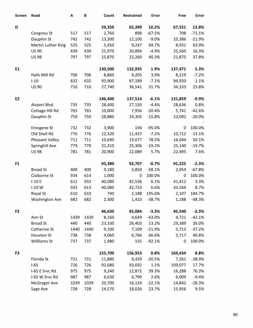
90

Screen Road A B Count Restrained Error Free Error

D 59,350 65,399 10.2% 67,551 13.8%

Congress St 517 517 2,760 898 -67.5% 798 -71.1%

Dauphin St 742 742 13,300 12,100 -9.0% 10,386 -21.9%

Martin Luther King 525 525 5,450 9,247 69.7% 8,931 63.9%

US 90 439 439 21,970 20,894 -4.9% 25,560 16.3%

US 98 797 797 15,870 22,260 40.3% 21,875 37.8%

E1 130,500 132,935 1.9% 137,471 5.3%

Halls Mill Rd 706 706 8,860 9,205 3.9% 8,219 -7.2%

I-10 632 632 93,900 87,189 -7.1% 94,920 1.1%

US 90 710 710 27,740 36,541 31.7% 34,333 23.8%

E2 146,400 137,514 -6.1% 131,859 -9.9%

Airport Blvd 735 735 28,400 27,150 -4.4% 28,636 0.8%

Cottage Hill Rd 765 765 10,000 7,956 -20.4% 5,741 -42.6%

Dauphin St 759 759 28,880 24,305 -15.8% 23,092 -20.0%

Emogene St 732 732 3,900 194 -95.0% 0 -

100.0%

Old Shell Rd 776 776 12,320 11,437 -7.2% 10,712 -13.1%

Pleasant Valley 711 711 10,690 19,077 78.5% 16,044 50.1%

Springhill Ave 779 779 31,310 25,306 -19.2% 25,140 -19.7%

US 98 781 781 20,900 22,089 5.7% 22,495 7.6%

F1 93,380 92,707 -0.7% 91,225 -2.3%

Broad St 400 400 9,180 3,850 -58.1% 2,954 -67.8%

Claiborne St 934 614 1,000 0 100.0% 0 100.0%

I-10 E 612 932 40,080 42,536 6.1% 41,412 3.3%

I-10 W 933 613 40,080 42,723 6.6% 43,564 8.7%

Royal St 610 610 740 2,188 195.6% 2,107 184.7%

Washington Ave 682 682 2,300 1,410 -38.7% 1,188 -48.3%

F2 46,630 45,084 -3.3% 45,540 -2.3%

Ann St 1439 1439 8,160 4,649 -43.0% 4,721 -42.1%

Broad St 440 440 23,330 26,403 13.2% 29,389 26.0%

Catherine St 1440 1440 9,100 7,109 -21.9% 5,713 -37.2%

Houston St 738 738 4,060 6,766 66.6% 5,717 40.8%

Willliams St 737 737 1,980 155 -92.1% 0 100.0%

F3 155,700 156,953 0.8% 169,434 8.8%

Florida St 721 721 11,880 9,439 -20.5% 7,261 -38.9%

I-65 726 726 92,680 93,692 1.1% 109,077 17.7%

I-65 E Srvc Rd 975 975 9,240 12,872 39.3% 16,288 76.3%

I-65 W Srvc Rd 987 987 6,630 6,799 2.6% 6,009 -9.4%

McGregor Ave 1039 1039 20,700 16,124 -22.1% 14,842 -28.3%

Sage Ave 728 728 14,570 18,026 23.7% 15,956 9.5%

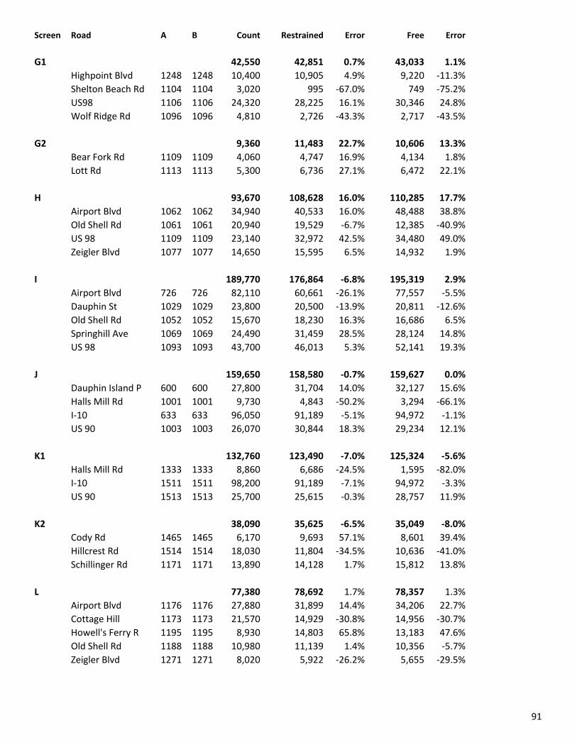
91

Screen Road A B Count Restrained Error Free Error

G1 42,550 42,851 0.7% 43,033 1.1%

Highpoint Blvd 1248 1248 10,400 10,905 4.9% 9,220 -11.3%

Shelton Beach Rd 1104 1104 3,020 995 -67.0% 749 -75.2%

US98 1106 1106 24,320 28,225 16.1% 30,346 24.8%

Wolf Ridge Rd 1096 1096 4,810 2,726 -43.3% 2,717 -43.5%

G2 9,360 11,483 22.7% 10,606 13.3%

Bear Fork Rd 1109 1109 4,060 4,747 16.9% 4,134 1.8%

Lott Rd 1113 1113 5,300 6,736 27.1% 6,472 22.1%

H 93,670 108,628 16.0% 110,285 17.7%

Airport Blvd 1062 1062 34,940 40,533 16.0% 48,488 38.8%

Old Shell Rd 1061 1061 20,940 19,529 -6.7% 12,385 -40.9%

US 98 1109 1109 23,140 32,972 42.5% 34,480 49.0%

Zeigler Blvd 1077 1077 14,650 15,595 6.5% 14,932 1.9%

I 189,770 176,864 -6.8% 195,319 2.9%

Airport Blvd 726 726 82,110 60,661 -26.1% 77,557 -5.5%

Dauphin St 1029 1029 23,800 20,500 -13.9% 20,811 -12.6%

Old Shell Rd 1052 1052 15,670 18,230 16.3% 16,686 6.5%

Springhill Ave 1069 1069 24,490 31,459 28.5% 28,124 14.8%

US 98 1093 1093 43,700 46,013 5.3% 52,141 19.3%

J 159,650 158,580 -0.7% 159,627 0.0%

Dauphin Island P 600 600 27,800 31,704 14.0% 32,127 15.6%

Halls Mill Rd 1001 1001 9,730 4,843 -50.2% 3,294 -66.1%

I-10 633 633 96,050 91,189 -5.1% 94,972 -1.1%

US 90 1003 1003 26,070 30,844 18.3% 29,234 12.1%

K1 132,760 123,490 -7.0% 125,324 -5.6%

Halls Mill Rd 1333 1333 8,860 6,686 -24.5% 1,595 -82.0%

I-10 1511 1511 98,200 91,189 -7.1% 94,972 -3.3%

US 90 1513 1513 25,700 25,615 -0.3% 28,757 11.9%

K2 38,090 35,625 -6.5% 35,049 -8.0%

Cody Rd 1465 1465 6,170 9,693 57.1% 8,601 39.4%

Hillcrest Rd 1514 1514 18,030 11,804 -34.5% 10,636 -41.0%

Schillinger Rd 1171 1171 13,890 14,128 1.7% 15,812 13.8%

L 77,380 78,692 1.7% 78,357 1.3%

Airport Blvd 1176 1176 27,880 31,899 14.4% 34,206 22.7%

Cottage Hill 1173 1173 21,570 14,929 -30.8% 14,956 -30.7%

Howell's Ferry R 1195 1195 8,930 14,803 65.8% 13,183 47.6%

Old Shell Rd 1188 1188 10,980 11,139 1.4% 10,356 -5.7%

Zeigler Blvd 1271 1271 8,020 5,922 -26.2% 5,655 -29.5%

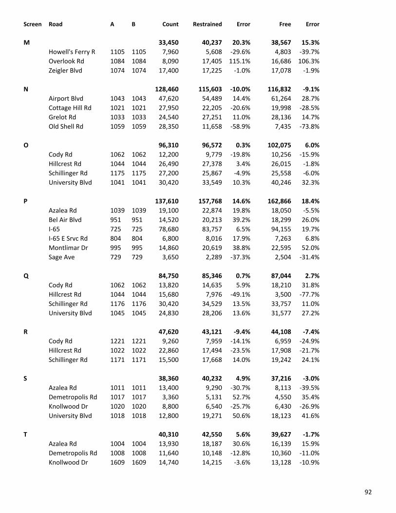
92

Screen Road A B Count Restrained Error Free Error

M 33,450 40,237 20.3% 38,567 15.3%

Howell's Ferry R 1105 1105 7,960 5,608 -29.6% 4,803 -39.7%

Overlook Rd 1084 1084 8,090 17,405 115.1% 16,686 106.3%

Zeigler Blvd 1074 1074 17,400 17,225 -1.0% 17,078 -1.9%

N 128,460 115,603 -10.0% 116,832 -9.1%

Airport Blvd 1043 1043 47,620 54,489 14.4% 61,264 28.7%

Cottage Hill Rd 1021 1021 27,950 22,205 -20.6% 19,998 -28.5%

Grelot Rd 1033 1033 24,540 27,251 11.0% 28,136 14.7%

Old Shell Rd 1059 1059 28,350 11,658 -58.9% 7,435 -73.8%

O 96,310 96,572 0.3% 102,075 6.0%

Cody Rd 1062 1062 12,200 9,779 -19.8% 10,256 -15.9%

Hillcrest Rd 1044 1044 26,490 27,378 3.4% 26,015 -1.8%

Schillinger Rd 1175 1175 27,200 25,867 -4.9% 25,558 -6.0%

University Blvd 1041 1041 30,420 33,549 10.3% 40,246 32.3%

P 137,610 157,768 14.6% 162,866 18.4%

Azalea Rd 1039 1039 19,100 22,874 19.8% 18,050 -5.5%

Bel Air Blvd 951 951 14,520 20,213 39.2% 18,299 26.0%

I-65 725 725 78,680 83,757 6.5% 94,155 19.7%

I-65 E Srvc Rd 804 804 6,800 8,016 17.9% 7,263 6.8%

Montlimar Dr 995 995 14,860 20,619 38.8% 22,595 52.0%

Sage Ave 729 729 3,650 2,289 -37.3% 2,504 -31.4%

Q 84,750 85,346 0.7% 87,044 2.7%

Cody Rd 1062 1062 13,820 14,635 5.9% 18,210 31.8%

Hillcrest Rd 1044 1044 15,680 7,976 -49.1% 3,500 -77.7%

Schillinger Rd 1176 1176 30,420 34,529 13.5% 33,757 11.0%

University Blvd 1045 1045 24,830 28,206 13.6% 31,577 27.2%

R 47,620 43,121 -9.4% 44,108 -7.4%

Cody Rd 1221 1221 9,260 7,959 -14.1% 6,959 -24.9%

Hillcrest Rd 1022 1022 22,860 17,494 -23.5% 17,908 -21.7%

Schillinger Rd 1171 1171 15,500 17,668 14.0% 19,242 24.1%

S 38,360 40,232 4.9% 37,216 -3.0%

Azalea Rd 1011 1011 13,400 9,290 -30.7% 8,113 -39.5%

Demetropolis Rd 1017 1017 3,360 5,131 52.7% 4,550 35.4%

Knollwood Dr 1020 1020 8,800 6,540 -25.7% 6,430 -26.9%

University Blvd 1018 1018 12,800 19,271 50.6% 18,123 41.6%

T 40,310 42,550 5.6% 39,627 -1.7%

Azalea Rd 1004 1004 13,930 18,187 30.6% 16,139 15.9%

Demetropolis Rd 1008 1008 11,640 10,148 -12.8% 10,360 -11.0%

Knollwood Dr 1609 1609 14,740 14,215 -3.6% 13,128 -10.9%

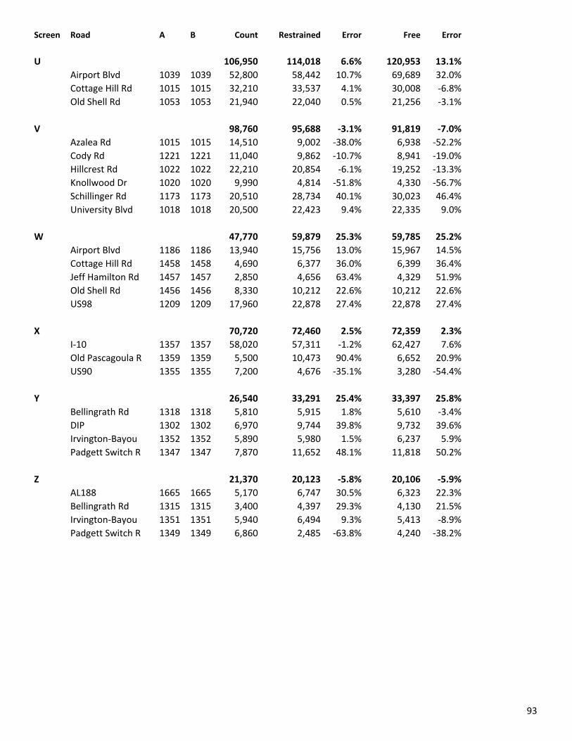
93

Screen Road A B Count Restrained Error Free Error

U 106,950 114,018 6.6% 120,953 13.1%

Airport Blvd 1039 1039 52,800 58,442 10.7% 69,689 32.0%

Cottage Hill Rd 1015 1015 32,210 33,537 4.1% 30,008 -6.8%

Old Shell Rd 1053 1053 21,940 22,040 0.5% 21,256 -3.1%

V 98,760 95,688 -3.1% 91,819 -7.0%

Azalea Rd 1015 1015 14,510 9,002 -38.0% 6,938 -52.2%

Cody Rd 1221 1221 11,040 9,862 -10.7% 8,941 -19.0%

Hillcrest Rd 1022 1022 22,210 20,854 -6.1% 19,252 -13.3%

Knollwood Dr 1020 1020 9,990 4,814 -51.8% 4,330 -56.7%

Schillinger Rd 1173 1173 20,510 28,734 40.1% 30,023 46.4%

University Blvd 1018 1018 20,500 22,423 9.4% 22,335 9.0%

W 47,770 59,879 25.3% 59,785 25.2%

Airport Blvd 1186 1186 13,940 15,756 13.0% 15,967 14.5%

Cottage Hill Rd 1458 1458 4,690 6,377 36.0% 6,399 36.4%

Jeff Hamilton Rd 1457 1457 2,850 4,656 63.4% 4,329 51.9%

Old Shell Rd 1456 1456 8,330 10,212 22.6% 10,212 22.6%

US98 1209 1209 17,960 22,878 27.4% 22,878 27.4%

X 70,720 72,460 2.5% 72,359 2.3%

I-10 1357 1357 58,020 57,311 -1.2% 62,427 7.6%

Old Pascagoula R 1359 1359 5,500 10,473 90.4% 6,652 20.9%

US90 1355 1355 7,200 4,676 -35.1% 3,280 -54.4%

Y 26,540 33,291 25.4% 33,397 25.8%

Bellingrath Rd 1318 1318 5,810 5,915 1.8% 5,610 -3.4%

DIP 1302 1302 6,970 9,744 39.8% 9,732 39.6%

Irvington-Bayou 1352 1352 5,890 5,980 1.5% 6,237 5.9%

Padgett Switch R 1347 1347 7,870 11,652 48.1% 11,818 50.2%

Z 21,370 20,123 -5.8% 20,106 -5.9%

AL188 1665 1665 5,170 6,747 30.5% 6,323 22.3%

Bellingrath Rd 1315 1315 3,400 4,397 29.3% 4,130 21.5%

Irvington-Bayou 1351 1351 5,940 6,494 9.3% 5,413 -8.9%

Padgett Switch R 1349 1349 6,860 2,485 -63.8% 4,240 -38.2%

94

Appendix A9 Trucks

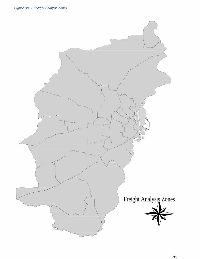
95

Figure A9- 1 Freight Analysis Zones

Freight Analysis Zones

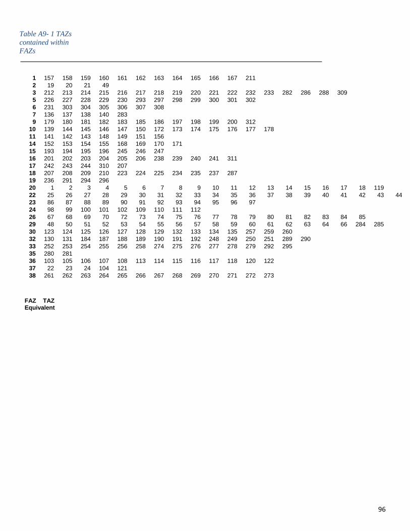
96

Table A9- 1 TAZs

contained within

FAZs

FAZ TAZ Equivalent

1 157 158 159 160 161 162 163 164 165 166 167 211 2 19 20 21 49 3 212 213 214 215 216 217 218 219 220 221 222 232 233 282 286 288 309 5 226 227 228 229 230 293 297 298 299 300 301 302 6 231 303 304 305 306 307 308 7 136 137 138 140 283 9 179 180 181 182 183 185 186 197 198 199 200 312

10 139 144 145 146 147 150 172 173 174 175 176 177 178 11 141 142 143 148 149 151 156 14 152 153 154 155 168 169 170 171 15 193 194 195 196 245 246 247 16 201 202 203 204 205 206 238 239 240 241 311 17 242 243 244 310 207 18 207 208 209 210 223 224 225 234 235 237 287 19 236 291 294 296 20 1 2 3 4 5 6 7 8 9 10 11 12 13 14 15 16 17 18 119

22 25 26 27 28 29 30 31 32 33 34 35 36 37 38 39 40 41 42 43 44 45 46 47 65 71

23 86 87 88 89 90 91 92 93 94 95 96 97 24 98 99 100 101 102 109 110 111 112 26 67 68 69 70 72 73 74 75 76 77 78 79 80 81 82 83 84 85 29 48 50 51 52 53 54 55 56 57 58 59 60 61 62 63 64 66 284 285 30 123 124 125 126 127 128 129 132 133 134 135 257 259 260 32 130 131 184 187 188 189 190 191 192 248 249 250 251 289 290 33 252 253 254 255 256 258 274 275 276 277 278 279 292 295 35 280 281 36 103 105 106 107 108 113 114 115 116 117 118 120 122 37 22 23 24 104 121 38 261 262 263 264 265 266 267 268 269 270 271 272 273

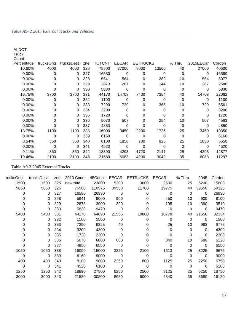
97

Table A9- 2 2015 External Trucks and Vehicles

ALDOT Truck Count Percentage trucksOrig trucksDest zne TOTCNT EECAR EETRUCKS % Thru 2015EECar Cordon

10.60% 4000 4000 326 75500 27000 8000 13500 40 27000 40500

0.00% 0 0 327 16580 0 0 0 0 0 16580

0.00% 0 0 328 5641 564 0 282 10 564 5077

0.00% 0 0 329 2873 287 0 144 10 287 2586

0.00% 0 0 330 5830 0 0 0 0 0 5830

16.75% 3700 3700 331 44170 14708 7400 7354 40 14708 22062

0.00% 0 0 332 1100 0 0 0 0 0 1100

0.00% 0 0 333 7290 729 0 365 10 729 6561

0.00% 0 0 334 3200 0 0 0 0 0 3200

0.00% 0 0 335 1720 0 0 0 0 0 1720

0.00% 0 0 336 5070 507 0 254 10 507 4563

0.00% 0 0 337 4850 0 0 0 0 0 4850

13.75% 1100 1100 338 16000 3450 2200 1725 25 3450 10350

0.00% 0 0 339 6160 0 0 0 0 0 6160

8.64% 350 350 340 8100 1850 700 925 25 1850 5550

0.00% 0 0 341 4520 0 0 0 0 0 4520

9.11% 860 860 342 18890 4293 1720 2147 25 4293 12877

19.46% 2100 2100 343 21580 6083 4200 3042 35 6083 11297

Table A9-3 2045 External Trucks

trucksOrig trucksDest zne 2010 Count 45Count EECAR EETRUCKS EECAR % Thru 2045 Cordon

1500 1500 325 newroad 23800 5200 3000 2600 25 5200 15600

5850 5850 326 75500 110575 39550 11700 19775 40 39550 59325

0 0 327 16580 26930 0 0 0 0 0 26930

0 0 328 5641 9000 900 0 450 10 900 8100

0 0 329 2873 3900 390 0 195 10 390 3510

0 0 330 5830 9470 0 0 0 0 0 9470

5400 5400 331 44170 64690 21556 10800 10778 40 21556 32334

0 0 332 1100 1500 0 0 0 0 0 1500

0 0 333 7290 9825 49 0 25 10 983 9776

0 0 334 3200 4300 0 0 0 0 0 4300

0 0 335 1720 2300 0 0 0 0 0 2300

0 0 336 5070 6800 680 0 340 10 680 6120

0 0 337 4850 6550 0 0 0 0 0 6550

1050 1050 338 16000 15000 3225 2100 1613 25 3225 9675

0 0 339 6160 9000 0 0 0 0 0 9000

400 400 340 8100 9800 2250 800 1125 25 2250 6750

0 0 341 4520 6100 0 0 0 0 0 6100

1250 1250 342 18890 27500 6250 2500 3125 25 6250 18750

3000 3000 343 21580 30800 8680 6000 4340 35 8680 16120

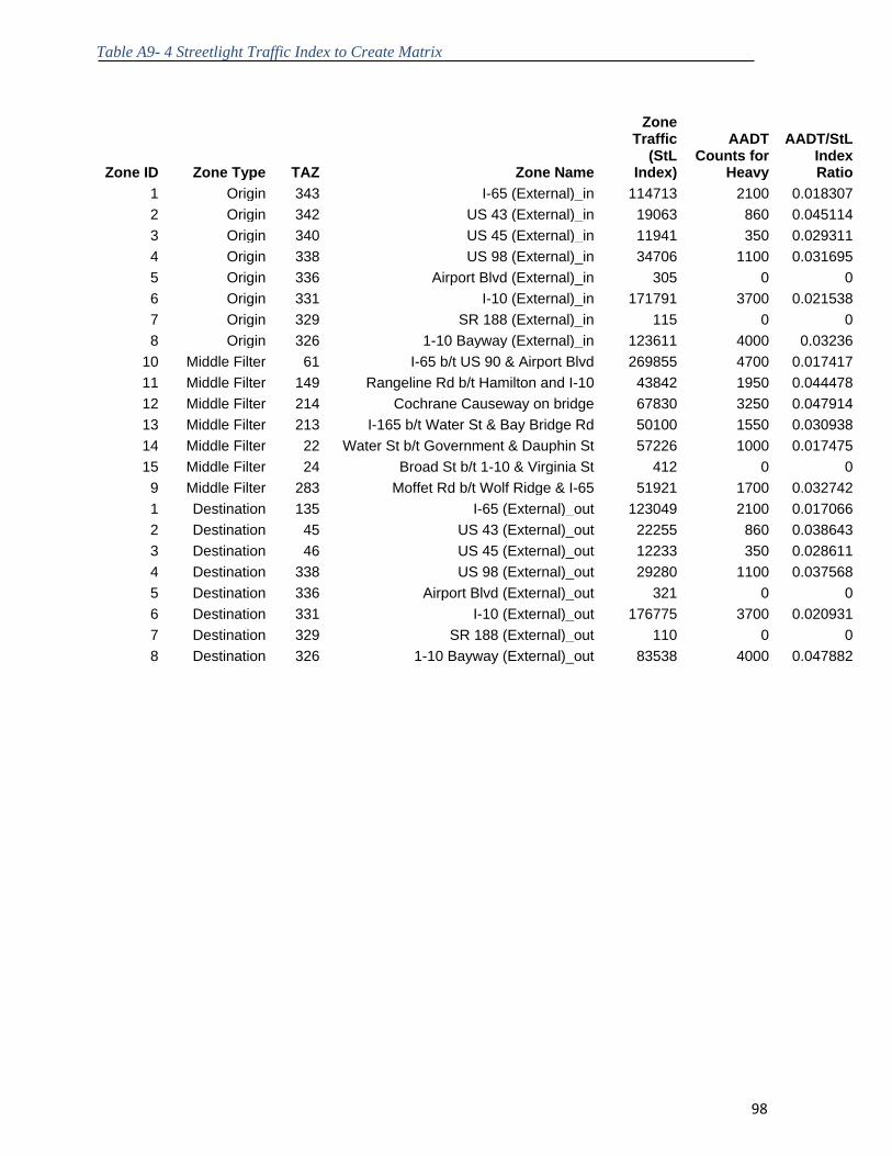
98

Table A9- 4 Streetlight Traffic Index to Create Matrix

Zone ID Zone Type TAZ Zone Name

Zone Traffic

(StL Index)

AADT Counts for

Heavy

AADT/StL Index Ratio

1 Origin 343 I-65 (External)_in 114713 2100 0.018307

2 Origin 342 US 43 (External)_in 19063 860 0.045114

3 Origin 340 US 45 (External)_in 11941 350 0.029311

4 Origin 338 US 98 (External)_in 34706 1100 0.031695

5 Origin 336 Airport Blvd (External)_in 305 0 0

6 Origin 331 I-10 (External)_in 171791 3700 0.021538

7 Origin 329 SR 188 (External)_in 115 0 0

8 Origin 326 1-10 Bayway (External)_in 123611 4000 0.03236

10 Middle Filter 61 I-65 b/t US 90 & Airport Blvd 269855 4700 0.017417

11 Middle Filter 149 Rangeline Rd b/t Hamilton and I-10 43842 1950 0.044478

12 Middle Filter 214 Cochrane Causeway on bridge 67830 3250 0.047914

13 Middle Filter 213 I-165 b/t Water St & Bay Bridge Rd 50100 1550 0.030938

14 Middle Filter 22 Water St b/t Government & Dauphin St 57226 1000 0.017475

15 Middle Filter 24 Broad St b/t 1-10 & Virginia St 412 0 0

9 Middle Filter 283 Moffet Rd b/t Wolf Ridge & I-65 51921 1700 0.032742

1 Destination 135 I-65 (External)_out 123049 2100 0.017066

2 Destination 45 US 43 (External)_out 22255 860 0.038643

3 Destination 46 US 45 (External)_out 12233 350 0.028611

4 Destination 338 US 98 (External)_out 29280 1100 0.037568

5 Destination 336 Airport Blvd (External)_out 321 0 0

6 Destination 331 I-10 (External)_out 176775 3700 0.020931

7 Destination 329 SR 188 (External)_out 110 0 0

8 Destination 326 1-10 Bayway (External)_out 83538 4000 0.047882

99

APPENDIX A-10

Origin Destination Study for Mobile County - SARPC

December 31, 2012

Mr. Kevin Harrison, P.T.P. Director, Transportation Planning

South Alabama Regional Planning Comm. www.sarpc.org

www.mobilempo.org (251) 433-6541

AirSage, Inc. | 1330 Spring Street NW | Suite 400 | Atlanta, GA 30309

www.airsage.com | 678-387-1310

100

1.0 INTRODUCTION

AirSage, an Atlanta based wireless information and data provider, has developed a new approach to gathering data about population mobility throughout a region. AirSage analyzes anonymous location and movement of mobile devices, which is derived from wireless signaling data, to provide new insights into where populations, are, were or will be, and how they move about over time and in response to special events or disruptions to the roadway network.

With increasing fiscal constraints, limited resources, and growing management challenges, the need to prioritize investments has never been more pressing. Agencies must undertake extensive planning activities to better understand, among other things, travel demand and visitor demographics. This information provides a framework to guide decisions for actions, approve uses, and funding.

The purpose of this document is to describe the methodology used by AirSage to determine Origin and Destination and to calibrate the SARPC Travel demand model and to present the results in Summary.

2.0 AIRSAGE TECHNOLOGY

AirSage provides population location, movement, and traffic information derived from analysis of wireless (and in particular, cellular phone) signaling data. Combining patented and proprietary data collection and analysis technologies with signaling data from wireless carriers, AirSage has developed and deployed a secure data collection and reporting network with over 100 million mobile “sensors” that provide unprecedented visibility into where groups of people are, where they were, where they are likely to be, and how they move from one area to another.

AirSage’s WiSE (Wireless Signal Extraction) technology extracts data from wireless carrier networks, as generated by devices in the normal course of operation. Mobile devices frequently communicate with the network through control channel messages, both during use and when the mobile is in idle mode. The frequency and nature of the signaling data varies based on the network equipment used to provide cellular service to the area. The WiSE technology anonymizes the data stream (ensuring user privacy) and performs multiple stages of analysis to monitor the location and movement of the mobile devices (and thus the population of mobile users).

101

© 2012 AirSage, Inc.

3.0 AIRSAGE STUDY METHODOLOGY

AirSage uses a modular, multi-step methodology to derive useful information and analytics from wireless signaling data provided by its wireless carrier partners.

The core functional components are listed below, and further described throughout the remainder of this document.

AirSage PDE + Post-Process: Generates time-stamped locations (lat/long) for each mobile device (e.g. a cellphone), utilizing the network signaling data generated each time a mobile device interacts with the mobile network. Post-processing is applied to refine the raw location data, yielding Processed Sightings.

Activity Point Generation: Processed Sightings are grouped into uniform “grid cells” or “Grids” (rectangles typically 1000 meters on a side), which are the basic geographical unit used by AirSage to analyze movement of mobile devices over time. Collectively, a series of one or more time-consecutive sightings within a single Grid represent a single Activity Point. Additional attributes assigned to the Activity Point characterize the device’s movement (or “Activity”) relative to that Grid. For example, has the device just completed a trip? Is it just passing through?

TAZ Assignment: For each particular study, one or more Traffic Analysis Zones (TAZ) are defined by geographical boundaries that define a particular area (e.g. a neighborhood) or venue (e.g. a sports stadium, a park, etc.). In TAZ Assignment, each Activity Point is assigned to a that contains it.

Data Expansion: Using several factors, such as the relative mobile device penetration of AirSage partner carriers vs. the full population, US Census data, visibility (subscriber sighting frequency), and others, the TAZ Count sample data is expanded to reflect the actual Trip Count that would be expected to be observed in the field (i.e. for the total population).

Post Analysis: To meet specific project requirements, additional analysis may be applied to further characterize the Trips to a given TAZ. Examples include Origin (determined using subscriber Home/Work Tables), visit duration (how long did a given Visitor dwell in the TAZ?), and visit frequency (over a given time period, how often did a given Visitor visit the TAZ?). The extent and granularity of these insights depends on a variety of factors including the time period studied, sample size relative to the universe of potential trips, and others.

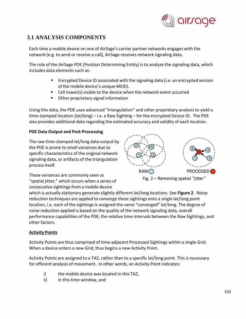
102

3.1 ANALYSIS COMPONENTS

Each time a mobile device on one of AirSage’s carrier partner networks engages with the network (e.g. to send or receive a call), AirSage receives network signaling data.

The role of the AirSage PDE (Position Determining Entity) is to analyze the signaling data, which includes data elements such as:

▪ Encrypted Device ID associated with the signaling data (i.e. an encrypted version of the mobile device’s unique MEID).

▪ Cell tower(s) visible to the device when the network event occurred ▪ Other proprietary signal information

Using this data, the PDE uses advanced “triangulation” and other proprietary analysis to yield a time-stamped location (lat/long) – i.e. a Raw Sighting – for the encrypted Device ID. The PDE also provides additional data regarding the estimated accuracy and validity of each location.

PDE Data Output and Post-Processing

The raw time-stamped lat/long data output by the PDE is prone to small variances due to specific characteristics of the original network signaling data, or artifacts of the triangulation process itself.

These variances are commonly seen as “spatial jitter,” which occurs when a series of consecutive sightings from a mobile device which is actually stationary generate slightly different lat/long locations. See Figure 2. Noise reduction techniques are applied to converge these sightings onto a single lat/long point location, i.e. each of the sightings is assigned the same “converged” lat/long. The degree of noise reduction applied is based on the quality of the network signaling data, overall performance capabilities of the PDE, the relative time intervals between the Raw Sightings, and other factors.

Activity Points

Activity Points are thus comprised of time-adjacent Processed Sightings within a single Grid. When a device enters a new Grid, thus begins a new Activity Point.

Activity Points are assigned to a TAZ, rather than to a specific lat/long point. This is necessary for efficient analysis of movement. In other words, an Activity Point indicates:

i) the mobile device was located in this TAZ, ii) in this time window, and

103

© 2012 AirSage, Inc.

iii) the device was either stationary or moving (or “uncertain”) in this TAZ and time window.

3.1.1 Data Output

Because they encompass multiple Processed Sightings, the output for Activity Points includes time duration, i.e. the difference between when the device entered that Grid, and when it left the Grid. These durations can be quite long, for example, when the device goes home after work and remains there overnight.

While not required specifically to derive Trip Counts, additional attributes are assigned to the Activity Point to characterize the device’s status or movement (i.e. “Activity”) relative to that Grid. For example, has the device just completed a trip (i.e. an “End Point”)? Is the device in motion, pasting through this Grid on the way to a different destination (i.e. a “Transient Point”)?

3.1.2 Subscriber Visibility

Also generated with Activity Points are Subscriber Visibility statistics. These stats deal with how frequently (or not) a given mobile device is visible to AirSage during the course of a day. Visibility tables are generally built using 15-minute intervals. This information becomes an input for Data Expansion.

3.1.3 Subscriber Home & Work Assignments

Also generated with Activity Points are the Home and Work census block groups for each mobile device. These are determined by observing device movement patterns over time. This information becomes an input for Data Expansion and other analysis.

3.2 TAZ (Traffic Analysis Zone) Assignment

3.2.1 Overview

A TAZ is simply a defined geographical boundary, usually associated with an area of interest (e.g. a neighborhood) or a business district (e.g. a sports stadium, a park, a retail location and surrounding buffer zone, etc.). TAZ definitions are typically provided via a GIS shapefile.

In TAZ Assignment, each Activity Point record is assigned, based on its Grid or raw location, to the TAZ boundary that contains that location.

104

3.3 Data Expansion

As indicated, the Trip Count output (across all mobile devices available on AirSage carrier partner networks) represents a sample Trip Count. This sample count represents only a portion of the total population of mobile devices and visitors to the TAZ.

To provide a full population Trip Counts, the sample data must be expanded. This expansion is accomplished using the following:

3.3.1 Determining the mobile devices’ “Home Location” Dividing the mobile device counts for a given “Home” census block group into US Census Population data for the same area yields a “Penetration Factor” – essentially a multiplier to apply to the sample data.

3.3.2 Optional: If the Trip Count is to report “vehicle” visits, rather than “people” visits, the count must be scaled to reflect average per-vehicle occupancy. Because AirSage counts mobile devices rather than vehicles, multiple occupants present in a vehicle will skew the count numbers higher. Dividing the AirSage mobile device counts by the average vehicle occupancy translates the output to vehicle counts.

3.3.3 Visibility Factors – how often, and at what intervals, a given device is “seen” by AirSage – are used to tune the expansion algorithms.

3.4 Post-Processing

Post-processing of Visitor Count data can yield valuable additional insights for a TAZ. Examples include Trip Origin (determined using subscriber Home/Work Tables), visit duration (how long did a given Visitor dwell in the TAZ?), and visit frequency (over a given time period, how often did a given Visitor visit the TAZ?).

The extent and granularity of these insights can only be determined after the Trip Count analysis is complete, as they depend on output data characteristics including the time period studied, and the effective sample size relative to the universe of potential Trips. The “density” of visitor Home locations is also an important consideration. For example, do Trips come from all over the country (as they might for a tourist destination), or do they come primarily from a local area (as they might for a shopping mall).

4.0 PROJECT SPECIFICS

AirSage partnered with Alliance Transportation Group for the actual calibration process. Their report is included herein in Appendix A

105

TECHNICAL MEMORANDUM

DATE: December 28, 2012

TO: Kevin Harrison, SARPC

CC: JD Allen

FROM: Jim Harvey

RE: SARPC Trip Distribution Model Calibration and Validation

This memorandum provides a description of the methodology and outcomes of the calibration of the

SARPC trip distribution model using trip ends derived from cell phone data for June 2012. Although the

scope only called for calibration of the trip distribution model, Alliance also validated the traffic assignment

model as a quality assurance check that the trip distribution tables produced by the calibrated model were

not only statistically reasonable, but also provided realistic inputs to support performance of downstream

model components. The following sections provide a description of the data inputs and methodology

used in calibrating and validating of the selected components of the SARPC travel demand model (TDM)

along with a summary of the outcomes of the process.

Data Inputs

This section provides a summary description of the cell phone data used in the calibration effort. A more

complete technical description of the data collection methodology, sampling plan, data reduction and

sample expansion is contained in the technical memorandum on cell phone data development prepared by

Airsage, the data vendor.

Airsage assembled sample cell phone transaction data from participating cell phone service providers for

the month of June 2012, and identified transactions being carried out by likely trip makers in the SARPC

study area. From this data, Airsage aggregated estimated linked trip origin destination zonal pairs for each

of the trips identified.

Airsage then used proprietary data analysis algorithms to impute a trip purpose for each of the identified

trips in the sample. Primary trip purposes defined in this manner included Home‐Based Work (HBW);

Home‐Based Other (HBO); and Non Home‐Based (NHB). Table 1 shows a comparison of the trips

obtained to the previous Mobile MPO TDM and the proportion of trips by purpose compared to NCHRP

reported typical ranges.

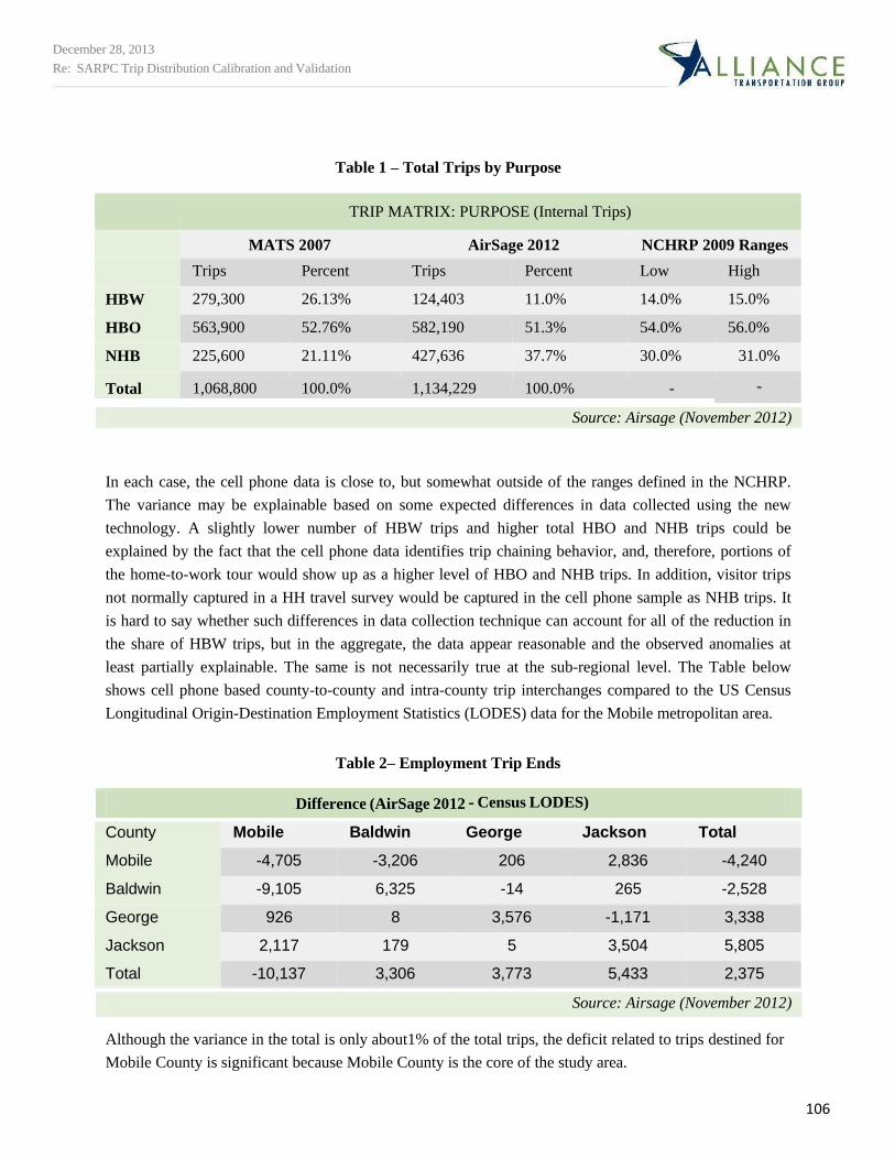
106

Table 1 – Total Trips by Purpose

TRIP MATRIX: PURPOSE (Internal Trips)

MATS 2007 AirSage 2012 NCHRP 2009 Ranges

Trips Percent Trips Percent Low High

HBW 279,300 26.13% 124,403 11.0% 14.0% 15.0%

HBO 563,900 52.76% 582,190 51.3% 54.0% 56.0%

NHB 225,600 21.11% 427,636 37.7% 30.0% 31.0%

Total 1,068,800 100.0% 1,134,229 100.0% - -

In each case, the cell phone data is close to, but somewhat outside of the ranges defined in the NCHRP.

The variance may be explainable based on some expected differences in data collected using the new

technology. A slightly lower number of HBW trips and higher total HBO and NHB trips could be

explained by the fact that the cell phone data identifies trip chaining behavior, and, therefore, portions of

the home-to-work tour would show up as a higher level of HBO and NHB trips. In addition, visitor trips

not normally captured in a HH travel survey would be captured in the cell phone sample as NHB trips. It

is hard to say whether such differences in data collection technique can account for all of the reduction in

the share of HBW trips, but in the aggregate, the data appear reasonable and the observed anomalies at

least partially explainable. The same is not necessarily true at the sub-regional level. The Table below

shows cell phone based county-to-county and intra-county trip interchanges compared to the US Census

Longitudinal Origin-Destination Employment Statistics (LODES) data for the Mobile metropolitan area.

Table 2– Employment Trip Ends

County Mobile Baldwin George Jackson Total

Mobile -4,705 -3,206 206 2,836 -4,240

Baldwin -9,105 6,325 -14 265 -2,528

George 926 8 3,576 -1,171 3,338

Jackson 2,117 179 5 3,504 5,805

Total -10,137 3,306 3,773 5,433 2,375

Although the variance in the total is only about1% of the total trips, the deficit related to trips destined for

Mobile County is significant because Mobile County is the core of the study area.

Source: Airsage (November 2012)

Difference (AirSage 2012 ‐ Census LODES)

Source: Airsage (November 2012)

December 28, 2013

Re: SARPC Trip Distribution Calibration and Validation

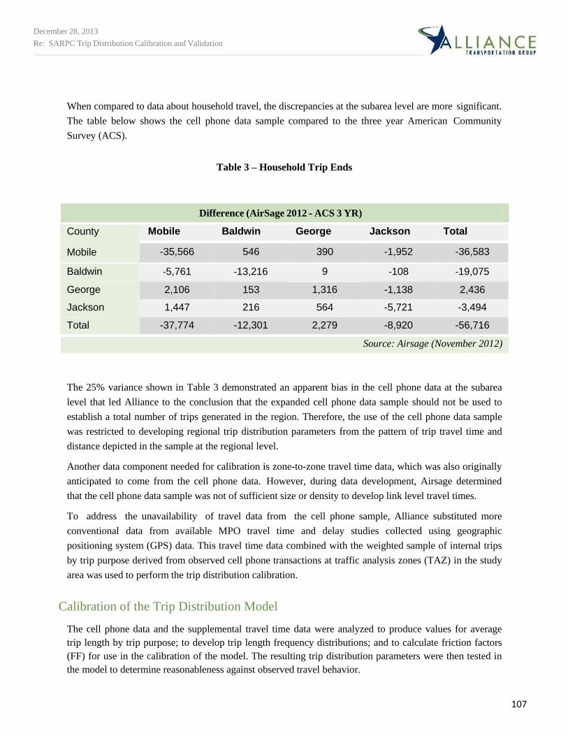
107

When compared to data about household travel, the discrepancies at the subarea level are more significant.

The table below shows the cell phone data sample compared to the three year American Community

Survey (ACS).

Table 3 – Household Trip Ends

County Mobile Baldwin George Jackson Total

Mobile -35,566 546 390 -1,952 -36,583

Baldwin ‐5,761 ‐13,216 9 ‐108 ‐19,075

George 2,106 153 1,316 -1,138 2,436

Jackson 1,447 216 564 -5,721 -3,494

Total -37,774 -12,301 2,279 -8,920 -56,716

The 25% variance shown in Table 3 demonstrated an apparent bias in the cell phone data at the subarea

level that led Alliance to the conclusion that the expanded cell phone data sample should not be used to

establish a total number of trips generated in the region. Therefore, the use of the cell phone data sample

was restricted to developing regional trip distribution parameters from the pattern of trip travel time and

distance depicted in the sample at the regional level.

Another data component needed for calibration is zone-to-zone travel time data, which was also originally

anticipated to come from the cell phone data. However, during data development, Airsage determined

that the cell phone data sample was not of sufficient size or density to develop link level travel times.

To address the unavailability of travel data from the cell phone sample, Alliance substituted more

conventional data from available MPO travel time and delay studies collected using geographic

positioning system (GPS) data. This travel time data combined with the weighted sample of internal trips

by trip purpose derived from observed cell phone transactions at traffic analysis zones (TAZ) in the study

area was used to perform the trip distribution calibration.

Calibration of the Trip Distribution Model

The cell phone data and the supplemental travel time data were analyzed to produce values for average

trip length by trip purpose; to develop trip length frequency distributions; and to calculate friction factors

(FF) for use in the calibration of the model. The resulting trip distribution parameters were then tested in

the model to determine reasonableness against observed travel behavior.

Difference (AirSage 2012 ‐ ACS 3 YR)

Source: Airsage (November 2012)

December 28, 2013

Re: SARPC Trip Distribution Calibration and Validation

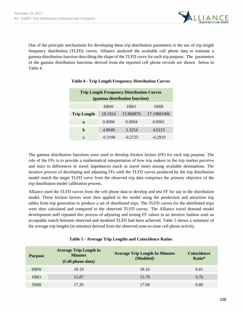
108

One of the principle mechanisms for developing these trip distribution parameters is the use of trip length

frequency distribution (TLFD) curves. Alliance analyzed the available cell phone data to estimate a

gamma distribution function describing the shape of the TLFD curve for each trip purpose. The parameters

of the gamma distribution functions derived from the reported cell phone records are shown below in

Table 4.

Table 4 - Trip Length Frequency Distribution Curves

Trip Length Frequency Distribution Curves

(gamma distribution function)

HBW HBO NHB

Trip Length 18.1924 15.868876 17.19881006

a 0.0000 0.0004 0.0001

b 4.8049 3.3254 4.0215

c -0.3190 -0.2725 -0.2919

The gamma distribution functions were used to develop friction factors (FF) for each trip purpose. The

role of the FFs is to provide a mathematical interpretation of how trip makers in the trip market perceive

and react to differences in travel impedances (such as travel time) among available destinations. The

iterative process of developing and adjusting FFs until the TLFD curves produced by the trip distribution

model match the target TLFD curve from the observed trip data comprises the primary objective of the

trip distribution model calibration process.

Alliance used the TLFD curves from the cell phone data to develop and test FF for use in the distribution

model. These friction factors were then applied in the model using the production and attraction trip

tables from trip generation to produce a set of distributed trips. The TLFD curves for the distributed trips

were then calculated and compared to the observed TLFD curves. The Alliance travel demand model

development staff repeated this process of adjusting and testing FF values in an iterative fashion until an

acceptable match between observed and modeled TLFD had been achieved. Table 5 shows a summary of

the average trip lengths (in minutes) derived from the observed zone-to-zone cell phone activity.

Table 5 - Average Trip Lengths and Coincidence Ratios

Purpose

Average Trip Length in

Minutes

(Cell phone data)

Average Trip Length In Minutes

(Modeled)

Coincidence

Ratio*

HBW 18.19 18.16 0.81

HBO 15.87 15.79 0.76

NHB 17.20 17.09 0.80

December 28, 2013

Re: SARPC Trip Distribution Calibration and Validation

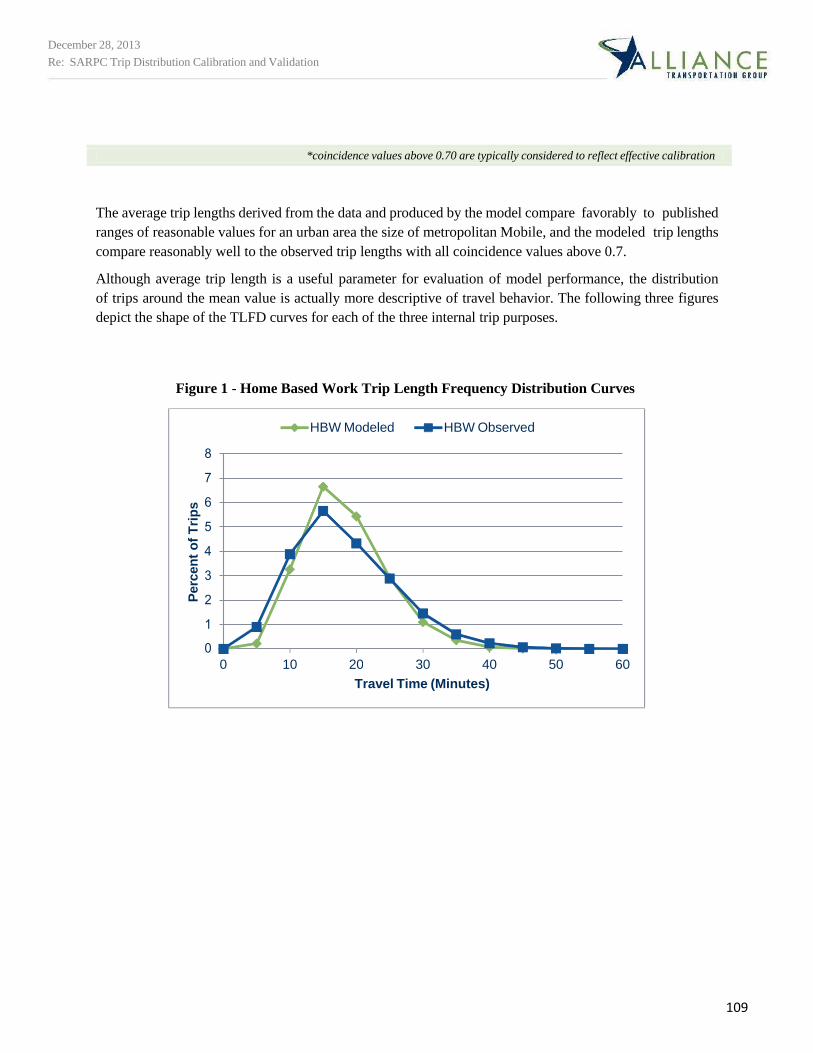
109

The average trip lengths derived from the data and produced by the model compare favorably to published

ranges of reasonable values for an urban area the size of metropolitan Mobile, and the modeled trip lengths

compare reasonably well to the observed trip lengths with all coincidence values above 0.7.

Although average trip length is a useful parameter for evaluation of model performance, the distribution

of trips around the mean value is actually more descriptive of travel behavior. The following three figures

depict the shape of the TLFD curves for each of the three internal trip purposes.

Figure 1 - Home Based Work Trip Length Frequency Distribution Curves

*coincidence values above 0.70 are typically considered to reflect effective calibration

December 28, 2013

Re: SARPC Trip Distribution Calibration and Validation

HBW Modeled HBW Observed

0 10 20 30 40 50 60

Travel Time (Minutes)

Perc

en

t o

f T

rip

s

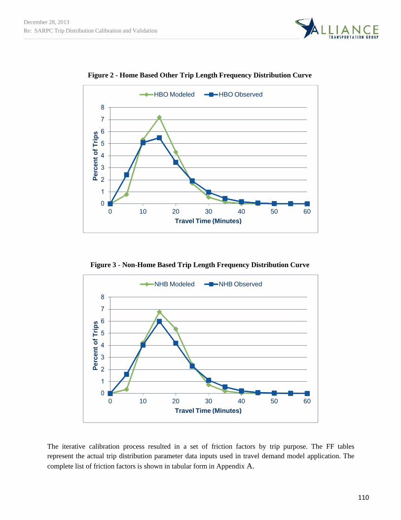
110

Figure 2 - Home Based Other Trip Length Frequency Distribution Curve

Figure 3 - Non-Home Based Trip Length Frequency Distribution Curve

The iterative calibration process resulted in a set of friction factors by trip purpose. The FF tables

represent the actual trip distribution parameter data inputs used in travel demand model application. The

complete list of friction factors is shown in tabular form in Appendix A.

December 28, 2013

Re: SARPC Trip Distribution Calibration and Validation

HBO Modeled HBO Observed

0 10 20 30 40 50 60

Travel Time (Minutes)

NHB Modeled NHB Observed

0 10 20 30 40 50 60

Travel Time (Minutes)

Perc

en

t o

f T

rip

s

Perc

en

t o

f T

rip

s

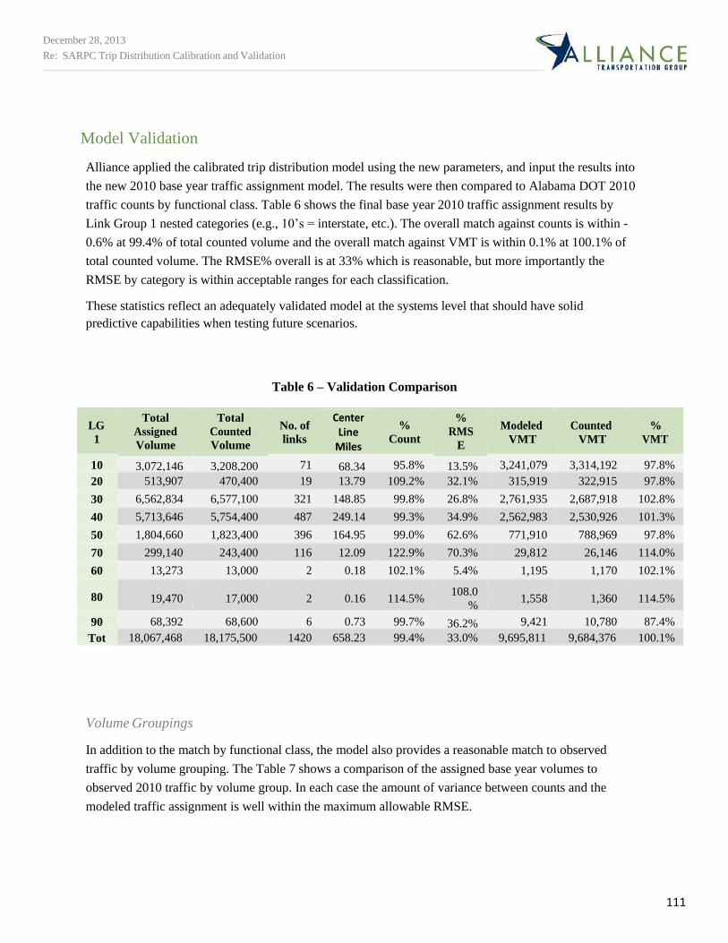
111

Model Validation

Alliance applied the calibrated trip distribution model using the new parameters, and input the results into

the new 2010 base year traffic assignment model. The results were then compared to Alabama DOT 2010

traffic counts by functional class. Table 6 shows the final base year 2010 traffic assignment results by

Link Group 1 nested categories (e.g., 10’s = interstate, etc.). The overall match against counts is within -

0.6% at 99.4% of total counted volume and the overall match against VMT is within 0.1% at 100.1% of

total counted volume. The RMSE% overall is at 33% which is reasonable, but more importantly the

RMSE by category is within acceptable ranges for each classification.

These statistics reflect an adequately validated model at the systems level that should have solid

predictive capabilities when testing future scenarios.

Table 6 – Validation Comparison

LG

1

Total

Assigned

Volume

Total

Counted

Volume

No. of

links

Center Line

Miles

%

Count

%

RMS

E

Modeled

VMT

Counted

VMT

%

VMT

10 3,072,146 3,208,200 71 68.34 95.8% 13.5% 3,241,079 3,314,192 97.8%

20 513,907 470,400 19 13.79 109.2% 32.1% 315,919 322,915 97.8%

30 6,562,834 6,577,100 321 148.85 99.8% 26.8% 2,761,935 2,687,918 102.8%

40 5,713,646 5,754,400 487 249.14 99.3% 34.9% 2,562,983 2,530,926 101.3%

50 1,804,660 1,823,400 396 164.95 99.0% 62.6% 771,910 788,969 97.8%

70 299,140 243,400 116 12.09 122.9% 70.3% 29,812 26,146 114.0%

60 13,273 13,000 2 0.18 102.1% 5.4% 1,195 1,170 102.1%

80 19,470 17,000 2 0.16 114.5% 108.0

% 1,558 1,360 114.5%

90 68,392 68,600 6 0.73 99.7% 36.2% 9,421 10,780 87.4%

Tot 18,067,468 18,175,500 1420 658.23 99.4% 33.0% 9,695,811 9,684,376 100.1%

Volume Groupings

In addition to the match by functional class, the model also provides a reasonable match to observed

traffic by volume grouping. The Table 7 shows a comparison of the assigned base year volumes to

observed 2010 traffic by volume group. In each case the amount of variance between counts and the

modeled traffic assignment is well within the maximum allowable RMSE.

December 28, 2013

Re: SARPC Trip Distribution Calibration and Validation

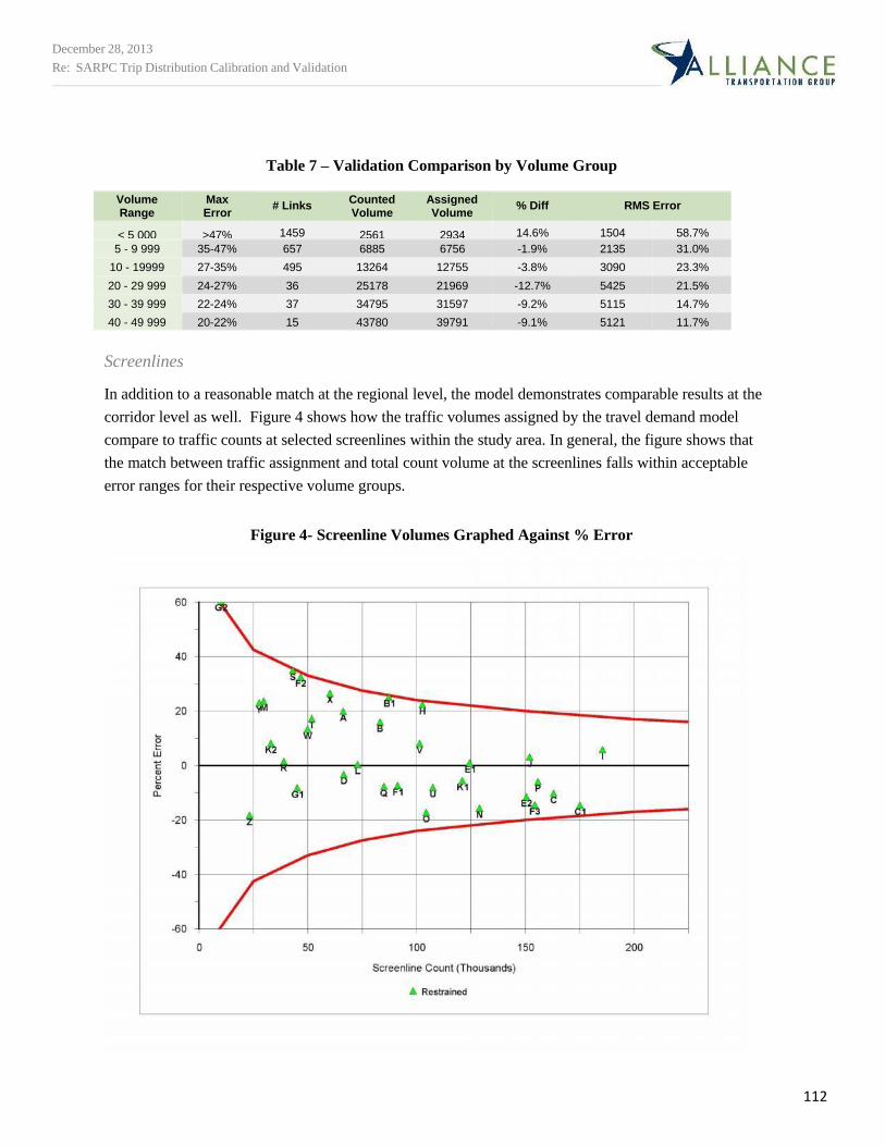
112

Table 7 – Validation Comparison by Volume Group

Volume Range

Max Error

# Links Counted Volume

Assigned Volume

% Diff RMS Error

< 5 000 >47% 1459 2561 2934 14.6% 1504 58.7%

5 - 9 999 35-47% 657 6885 6756 -1.9% 2135 31.0%

10 - 19999 27-35% 495 13264 12755 -3.8% 3090 23.3%

20 - 29 999 24-27% 36 25178 21969 -12.7% 5425 21.5%

30 - 39 999 22-24% 37 34795 31597 -9.2% 5115 14.7%

40 - 49 999 20-22% 15 43780 39791 -9.1% 5121 11.7%

Screenlines

In addition to a reasonable match at the regional level, the model demonstrates comparable results at the

corridor level as well. Figure 4 shows how the traffic volumes assigned by the travel demand model

compare to traffic counts at selected screenlines within the study area. In general, the figure shows that

the match between traffic assignment and total count volume at the screenlines falls within acceptable

error ranges for their respective volume groups.

Figure 4- Screenline Volumes Graphed Against % Error

December 28, 2013

Re: SARPC Trip Distribution Calibration and Validation

113

Conclusion

Although hampered somewhat by some unavailable data items and some perceived bias in the cell phone

sample, Alliance was able to use the available cell phone sample data to develop reasonable trip

distribution parameters and to calibrate a set of friction factors that meet acceptable statistical

benchmarks. When the trip distribution model was applied and the results input into the new 2010 base

year model, the traffic assignment validated well at both the regional and corridor level.

Based on the demonstrated performance of the Mobile MPO TDM 2010 base year model, SARPC can be

confident in the model’s predictive value for forecasting transportation system conditions on alternative

metropolitan transportation plan scenarios.

December 28, 2013

Re: SARPC Trip Distribution Calibration and Validation

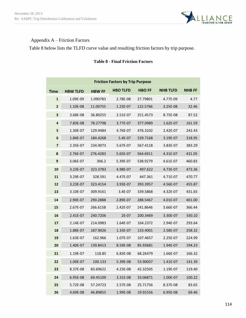
114

Appendix A – Friction Factors

Table 8 below lists the TLFD curve value and resulting friction factors by trip purpose.

Table 8 - Final Friction Factors

Time HBW TLFD HBW FF HBO TLFD HBO FF NHB TLFD NHB FF

1 1.09E-09 1.090783 2.78E-08 27.79801 4.77E-09 4.77

2 1.10E-08 11.00755 1.23E-07 122.5766 3.25E-08 32.46

3 3.68E-08 36.80255 2.51E-07 251.4573 8.75E-08 87.52

4 7.83E-08 78.27798 3.77E-07 377.0989 1.62E-07 161.59

5 1.30E-07 129.9484 4.76E-07 476.3102 2.42E-07 242.43

6 1.84E-07 184.4268 5.4E-07 539.7168 3.19E-07 318.95

7 2.35E-07 234.9073 5.67E-07 567.4118 3.83E-07 383.29

8 2.76E-07 276.4283 5.65E-07 564.6911 4.31E-07 431.05

9 3.06E-07 306.2 5.39E-07 538.9279 4.61E-07 460.83

10 3.23E-07 323.3783 4.98E-07 497.622 4.73E-07 473.36

11 3.29E-07 328.591 4.47E-07 447.361 4.71E-07 470.77

12 3.23E-07 323.4154 3.93E-07 393.3957 4.56E-07 455.87

13 3.10E-07 309.9161 3.4E-07 339.5868 4.32E-07 431.65

14 2.90E-07 290.2888 2.89E-07 288.5467 4.01E-07 401.00

15 2.67E-07 266.6158 2.42E-07 241.8646 3.66E-07 366.44

16 2.41E-07 240.7206 2E-07 200.3469 3.30E-07 330.10

17 2.14E-07 214.0983 1.64E-07 164.2372 2.94E-07 293.64

18 1.88E-07 187.9026 1.33E-07 133.4001 2.58E-07 258.32

19 1.63E-07 162.966 1.07E-07 107.4657 2.25E-07 224.99

20 1.40E-07 139.8413 8.59E-08 85.93681 1.94E-07 194.23

21 1.19E-07 118.85 6.83E-08 68.26479 1.66E-07 166.32

22 1.00E-07 100.133 5.39E-08 53.90037 1.41E-07 141.39

23 8.37E-08 83.69622 4.23E-08 42.32505 1.19E-07 119.40

24 6.95E-08 69.45109 3.31E-08 33.06871 1.00E-07 100.22

25 5.72E-08 57.24723 2.57E-08 25.71756 8.37E-08 83.65

26 4.69E-08 46.89855 1.99E-08 19.91556 6.95E-08 69.46

Friction Factors by Trip Purpose

December 28, 2013

Re: SARPC Trip Distribution Calibration and Validation

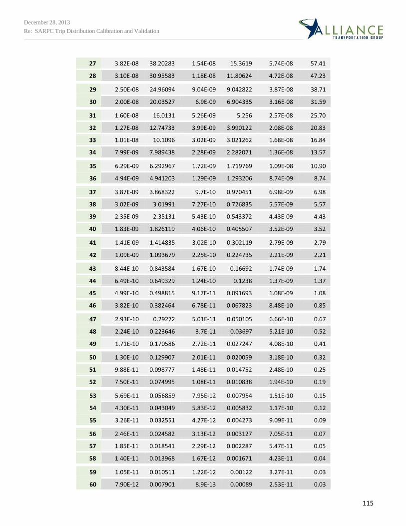
115

27 3.82E-08 38.20283 1.54E-08 15.3619 5.74E-08 57.41

28 3.10E-08 30.95583 1.18E-08 11.80624 4.72E-08 47.23

29 2.50E-08 24.96094 9.04E-09 9.042822 3.87E-08 38.71

30 2.00E-08 20.03527 6.9E-09 6.904335 3.16E-08 31.59

31 1.60E-08 16.0131 5.26E-09 5.256 2.57E-08 25.70

32 1.27E-08 12.74733 3.99E-09 3.990122 2.08E-08 20.83

33 1.01E-08 10.1096 3.02E-09 3.021262 1.68E-08 16.84

34 7.99E-09 7.989438 2.28E-09 2.282071 1.36E-08 13.57

35 6.29E-09 6.292967 1.72E-09 1.719769 1.09E-08 10.90

36 4.94E-09 4.941203 1.29E-09 1.293206 8.74E-09 8.74

37 3.87E-09 3.868322 9.7E-10 0.970451 6.98E-09 6.98

38 3.02E-09 3.01991 7.27E-10 0.726835 5.57E-09 5.57

39 2.35E-09 2.35131 5.43E-10 0.543372 4.43E-09 4.43

40 1.83E-09 1.826119 4.06E-10 0.405507 3.52E-09 3.52

41 1.41E-09 1.414835 3.02E-10 0.302119 2.79E-09 2.79

42 1.09E-09 1.093679 2.25E-10 0.224735 2.21E-09 2.21

43 8.44E-10 0.843584 1.67E-10 0.16692 1.74E-09 1.74

44 6.49E-10 0.649329 1.24E-10 0.1238 1.37E-09 1.37

45 4.99E-10 0.498815 9.17E-11 0.091693 1.08E-09 1.08

46 3.82E-10 0.382464 6.78E-11 0.067823 8.48E-10 0.85

47 2.93E-10 0.29272 5.01E-11 0.050105 6.66E-10 0.67

48 2.24E-10 0.223646 3.7E-11 0.03697 5.21E-10 0.52

49 1.71E-10 0.170586 2.72E-11 0.027247 4.08E-10 0.41

50 1.30E-10 0.129907 2.01E-11 0.020059 3.18E-10 0.32

51 9.88E-11 0.098777 1.48E-11 0.014752 2.48E-10 0.25

52 7.50E-11 0.074995 1.08E-11 0.010838 1.94E-10 0.19

53 5.69E-11 0.056859 7.95E-12 0.007954 1.51E-10 0.15

54 4.30E-11 0.043049 5.83E-12 0.005832 1.17E-10 0.12

55 3.26E-11 0.032551 4.27E-12 0.004273 9.09E-11 0.09

56 2.46E-11 0.024582 3.13E-12 0.003127 7.05E-11 0.07

57 1.85E-11 0.018541 2.29E-12 0.002287 5.47E-11 0.05

58 1.40E-11 0.013968 1.67E-12 0.001671 4.23E-11 0.04

59 1.05E-11 0.010511 1.22E-12 0.00122 3.27E-11 0.03

60 7.90E-12 0.007901 8.9E-13 0.00089 2.53E-11 0.03

December 28, 2013

Re: SARPC Trip Distribution Calibration and Validation

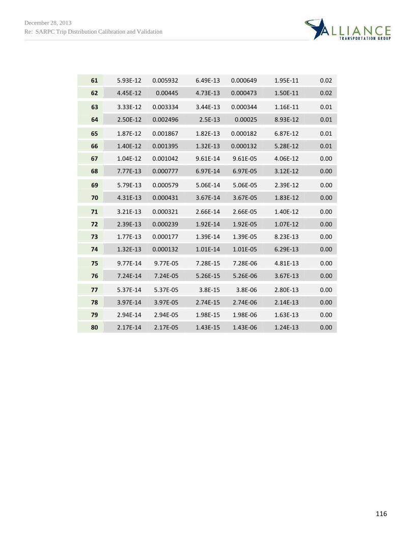
116

61 5.93E-12 0.005932 6.49E-13 0.000649 1.95E-11 0.02

62 4.45E-12 0.00445 4.73E-13 0.000473 1.50E-11 0.02

63 3.33E-12 0.003334 3.44E-13 0.000344 1.16E-11 0.01

64 2.50E-12 0.002496 2.5E-13 0.00025 8.93E-12 0.01

65 1.87E-12 0.001867 1.82E-13 0.000182 6.87E-12 0.01

66 1.40E-12 0.001395 1.32E-13 0.000132 5.28E-12 0.01

67 1.04E-12 0.001042 9.61E-14 9.61E-05 4.06E-12 0.00

68 7.77E-13 0.000777 6.97E-14 6.97E-05 3.12E-12 0.00

69 5.79E-13 0.000579 5.06E-14 5.06E-05 2.39E-12 0.00

70 4.31E-13 0.000431 3.67E-14 3.67E-05 1.83E-12 0.00

71 3.21E-13 0.000321 2.66E-14 2.66E-05 1.40E-12 0.00

72 2.39E-13 0.000239 1.92E-14 1.92E-05 1.07E-12 0.00

73 1.77E-13 0.000177 1.39E-14 1.39E-05 8.23E-13 0.00

74 1.32E-13 0.000132 1.01E-14 1.01E-05 6.29E-13 0.00

75 9.77E-14 9.77E-05 7.28E-15 7.28E-06 4.81E-13 0.00

76 7.24E-14 7.24E-05 5.26E-15 5.26E-06 3.67E-13 0.00

77 5.37E-14 5.37E-05 3.8E-15 3.8E-06 2.80E-13 0.00

78 3.97E-14 3.97E-05 2.74E-15 2.74E-06 2.14E-13 0.00

79 2.94E-14 2.94E-05 1.98E-15 1.98E-06 1.63E-13 0.00

80 2.17E-14 2.17E-05 1.43E-15 1.43E-06 1.24E-13 0.00

December 28, 2013

Re: SARPC Trip Distribution Calibration and Validation

117

Appendix A11 S.L.U.E.T.H. Methodology

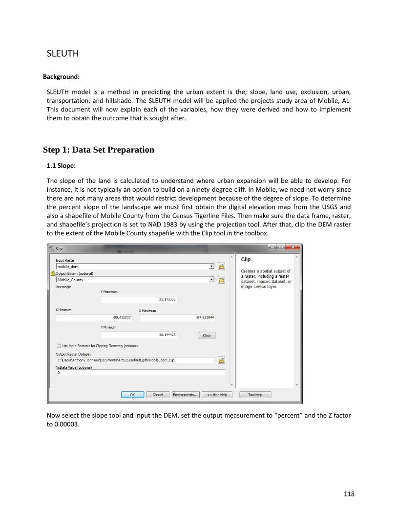
118

SLEUTH Background:

SLEUTH model is a method in predicting the urban extent is the; slope, land use, exclusion, urban, transportation, and hillshade. The SLEUTH model will be applied the projects study area of Mobile, AL. This document will now explain each of the variables, how they were derived and how to implement them to obtain the outcome that is sought after.

Step 1: Data Set Preparation

1.1 Slope:

The slope of the land is calculated to understand where urban expansion will be able to develop. For instance, it is not typically an option to build on a ninety-degree cliff. In Mobile, we need not worry since there are not many areas that would restrict development because of the degree of slope. To determine the percent slope of the landscape we must first obtain the digital elevation map from the USGS and also a shapefile of Mobile County from the Census Tigerline Files. Then make sure the data frame, raster, and shapefile’s projection is set to NAD 1983 by using the projection tool. After that, clip the DEM raster to the extent of the Mobile County shapefile with the Clip tool in the toolbox.

Now select the slope tool and input the DEM, set the output measurement to “percent” and the Z factor to 0.00003.

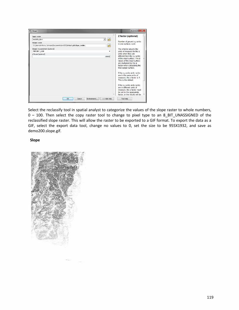
119

Select the reclassify tool in spatial analyst to categorize the values of the slope raster to whole numbers, 0 – 100. Then select the copy raster tool to change to pixel type to an 8_BIT_UNASSIGNED of the reclassified slope raster. This will allow the raster to be exported to a GIF format. To export the data as a GIF, select the export data tool, change no values to 0, set the size to be 955X1932, and save as demo200.slope.gif.

Slope

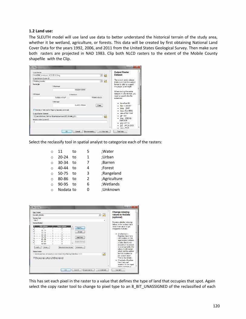
120

1.2 Land use:

The SLEUTH model will use land use data to better understand the historical terrain of the study area, whether it be wetland, agriculture, or forests. This data will be created by first obtaining National Land Cover Data for the years 1992, 2006, and 2011 from the United States Geological Survey. Then make sure both rasters are projected in NAD 1983. Clip both NLCD rasters to the extent of the Mobile County shapefile with the Clip.

Select the reclassify tool in spatial analyst to categorize each of the rasters:

o 11 to 5 ;Water

o 20-24 to 1 ;Urban

o 30-34 to 7 ;Barren

o 40-44 to 4 ;Forest

o 50-75 to 3 ;Rangeland

o 80-86 to 2 ;Agriculture

o 90-95 to 6 ;Wetlands

o Nodata to 0 ;Unknown

This has set each pixel in the raster to a value that defines the type of land that occupies that spot. Again select the copy raster tool to change to pixel type to an 8_BIT_UNASSIGNED of the reclassified of each

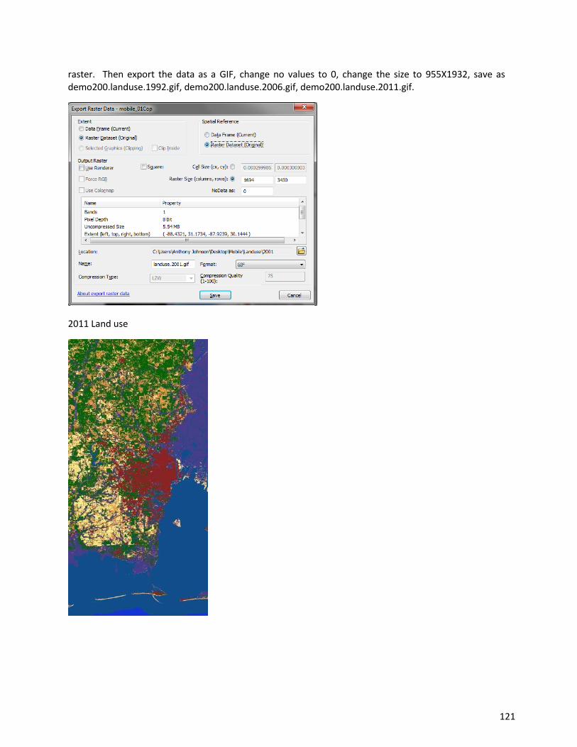
121

raster. Then export the data as a GIF, change no values to 0, change the size to 955X1932, save as demo200.landuse.1992.gif, demo200.landuse.2006.gif, demo200.landuse.2011.gif.

2011 Land use

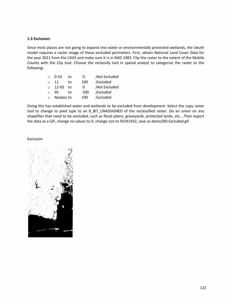
122

1.3 Exclusion:

Since most places are not going to expand into water or environmentally protected wetlands, the sleuth model requires a raster image of these excluded perimeters. First, obtain National Land Cover Data for the year 2011 from the USGS and make sure it is in NAD 1983. Clip the raster to the extent of the Mobile County with the Clip tool. Choose the reclassify tool in spatial analyst to categorize the raster to the following:

o 0-10 to 0 ;Not Excluded

o 11 to 100 ;Excluded

o 12-93 to 0 ;Not Excluded

o 95 to 100 ;Excluded

o Nodata to 100 ;Excluded

Doing this has established water and wetlands to be excluded from development. Select the copy raster tool to change to pixel type to an 8_BIT_UNASSIGNED of the reclassified raster. Do an union on any shapefiles that need to be excluded, such as flood plains, graveyards, protected lands, etc….Then export the data as a GIF, change no values to 0, change size to 955X1932, save as demo200.Excluded.gif.

Exclusion

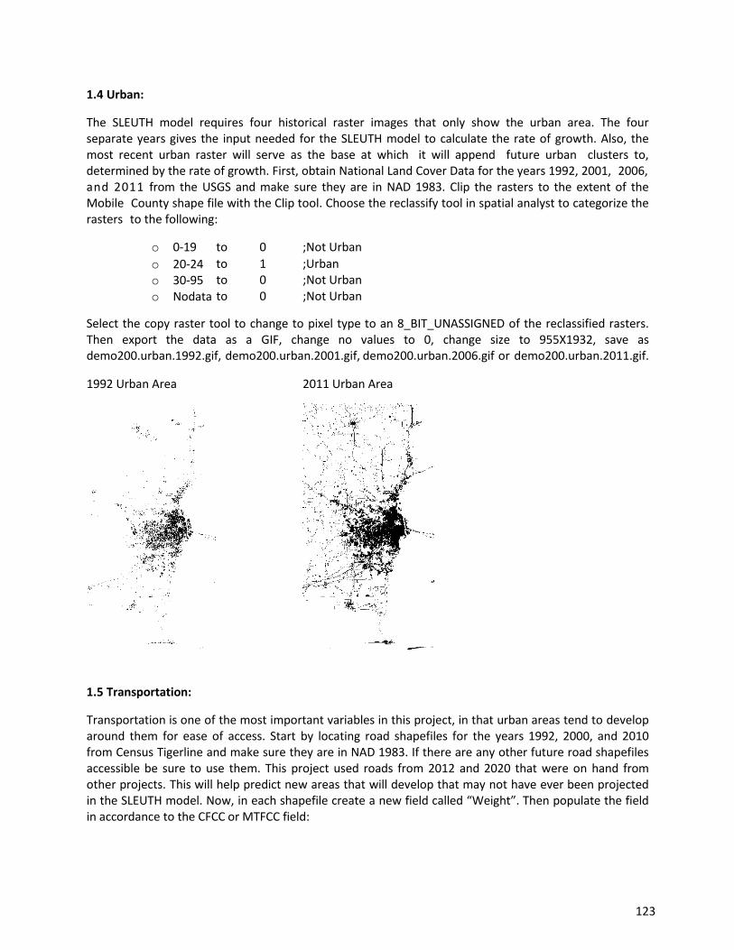
123

1.4 Urban:

The SLEUTH model requires four historical raster images that only show the urban area. The four separate years gives the input needed for the SLEUTH model to calculate the rate of growth. Also, the most recent urban raster will serve as the base at which it will append future urban clusters to, determined by the rate of growth. First, obtain National Land Cover Data for the years 1992, 2001, 2006, and 2011 from the USGS and make sure they are in NAD 1983. Clip the rasters to the extent of the Mobile County shape file with the Clip tool. Choose the reclassify tool in spatial analyst to categorize the rasters to the following:

o 0-19 to 0 ;Not Urban

o 20-24 to 1 ;Urban

o 30-95 to 0 ;Not Urban

o Nodata to 0 ;Not Urban

Select the copy raster tool to change to pixel type to an 8_BIT_UNASSIGNED of the reclassified rasters. Then export the data as a GIF, change no values to 0, change size to 955X1932, save as demo200.urban.1992.gif, demo200.urban.2001.gif, demo200.urban.2006.gif or demo200.urban.2011.gif.

1992 Urban Area 2011 Urban Area

1.5 Transportation:

Transportation is one of the most important variables in this project, in that urban areas tend to develop around them for ease of access. Start by locating road shapefiles for the years 1992, 2000, and 2010 from Census Tigerline and make sure they are in NAD 1983. If there are any other future road shapefiles accessible be sure to use them. This project used roads from 2012 and 2020 that were on hand from other projects. This will help predict new areas that will develop that may not have ever been projected in the SLEUTH model. Now, in each shapefile create a new field called “Weight”. Then populate the field in accordance to the CFCC or MTFCC field:

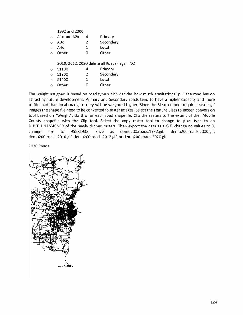
124

1992 and 2000

o A1x and A2x 4 Primary o A3x 2 Secondary o A4x 1 Local o Other 0 Other

2010, 2012, 2020 delete all RoadsFlags = NO

o S1100 4 Primary o S1200 2 Secondary

o S1400 1 Local

o Other 0 Other

The weight assigned is based on road type which decides how much gravitational pull the road has on attracting future development. Primary and Secondary roads tend to have a higher capacity and more traffic load than local roads, so they will be weighted higher. Since the Sleuth model requires raster gif images the shape file need to be converted to raster images. Select the Feature Class to Raster conversion tool based on “Weight”, do this for each road shapefile. Clip the rasters to the extent of the Mobile County shapefile with the Clip tool. Select the copy raster tool to change to pixel type to an 8_BIT_UNASSIGNED of the newly clipped rasters. Then export the data as a GIF, change no values to 0, change size to 955X1932, save as demo200.roads.1992.gif, demo200.roads.2000.gif, demo200.roads.2010.gif, demo200.roads.2012.gif, or demo200.roads.2020.gif.

2020 Roads

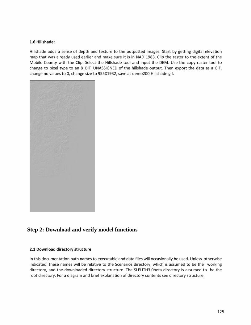
125

1.6 Hillshade:

Hillshade adds a sense of depth and texture to the outputted images. Start by getting digital elevation map that was already used earlier and make sure it is in NAD 1983. Clip the raster to the extent of the Mobile County with the Clip. Select the Hillshade tool and input the DEM. Use the copy raster tool to change to pixel type to an 8_BIT_UNASSIGNED of the hillshade output. Then export the data as a GIF, change no values to 0, change size to 955X1932, save as demo200.Hillshade.gif.

Step 2: Download and verify model functions

2.1 Download directory structure

In this documentation path names to executable and data files will occasionally be used. Unless otherwise indicated, these names will be relative to the Scenarios directory, which is assumed to be the working directory, and the downloaded directory structure. The SLEUTH3.0beta directory is assumed to be the root directory. For a diagram and brief explanation of directory contents see directory structure.

126

2.2 Download UGM3.0beta

The SLEUTH code may be acquired from the download page on this site. If an internet browser is used to download the file, be sure the filename extensions are not altered by the software.

2.2.1. Decompress file

To decompress the downloaded file from a command line interface:

prompt% unzip SLEUTH3.0beta.tar.gz

prompt% tar xvf SLEUTH3.0beta.tar

2.2.2. Compile code

Specifications for compiling SLEUTH3.0beta are set in the Makefile in the root directory. Variables include parallel processing and debug assert flags. Review the Makefile before compiling. The Makefiles in the three code directories (SLEUTH3.0beta, GD, and Whirlgif) all use the gcc C library compiler

To compile all libraries used by SLEUTH3.0beta:

(pathnames relative to the root directory SLEUTH3.0beta)

change directories into GD

prompt% cd GD

compile gd libraries

prompt% make

from GD change directories into Whirlgif

prompt% cd ../Whirlgif

compile whirlgif libraries

prompt% make

from Whirlgif change directories into the root directory

prompt% cd ..

compile SLEUTH3.0beta

prompt% make

2.3. Verify model execution

127

The downloaded scenario files will be set to run on a provided sample data set, demo_city. The scenario.demo200_test file is set to run in test mode, modeling urban land cover only. (To execute a test run modeling Anderson Level I land class types use the scenario.demo200_land_test file.) Many of the output image and statistic file flags are set to "YES". This is helpful to see what affect a certain set of coefficients is having upon the data, or simply confirm that the model is functioning properly. Examine the file scenario.demo200_test in the Scenarios directory. Note how the input and output path names, and input file names are set. This is how input and output is located for an application. Notice also the coefficient value settings. The *_START coefficient values will initialize the run. See also that the flags to write the average, standard deviation, and coefficient files are all set the "YES". These files will all be written to the output directory.

usage:

prompt% grow.exe <mode> <scenario file>

Allowable modes are:

calibrate

restart

test

predict

execute a test run: (from the Scenarios directory)

prompt% ../grow.exe test scenario.demo200_test

Data will be written to the screen showing application progress.

2.4. Check model output

All output files from a model execution will be written to the directory defined by the OUTPUT_DIR flag in the scenario.demo200_test file. In this case, the demo200_test directory located within the Output directory. The results from a test run on your machine and platform may be compared with ours to verify functionality and test performance. Results may vary slightly.

2.0 Calibration:

Calibration comes in three different stages. First is the coarse stage. The second stage is the fine stage. Lastly the final stage. Each one of these will have outputs that determine the values used for the

Step 2: Download and verify model functions

128

Step 3: Calibration Five coefficient values affect modeled urban growth of a study area. Known historical data is compared to simulated land cover in an effort to find the coefficient values that best model urban and related land cover change through time. These are measured using several Pearson r2 statistics, comparing measurements such as total number of urban pixels, edges, clusters and a spatial match comparison. For a more complete explanation see output statistic files.

Running SLEUTH in calibrate mode will perform brute force monte carlo runs through the historical data using every combination of the model coefficient values indicated. The CALIBRATION_*_START coefficient values (where "*" represents a coefficient type) will initialize the first simulation. A coefficient will then be increased by its _STEP value, and another simulation performed. This will continue until the coefficient _STOP value has been reached or exceeded. The incrementation will be repeated for all possible permutations of given ranges.

Calibration requires many (often thousands) of single simulations of land cover change. Because of this, output requirements can greatly add to the total application time. Many options are available for log and image file output during calibration. However, the fewer output files written, the more efficiently the code will run. It is important to understand the scenario file options to optimize it for your applications. To prevent overwriting, it is recommended to create, and in the scenario file point to, a unique output directory for each phase of model calibration and prediction.

Since the urban growth module of SLEUTH is its most basic component, the following instructions on how to calibrate the model will use urban growth only. The steps of calibration are the same when the Deltatron module is incorporated, but the output file control_stats.log will vary slightly. (For more information see: SLEUTH functions.

3.1 Set constants and verify

3.1.1 Create a scenario file for your data

The scenario.demo50_calibrate file is an example of how a file could be set up for first phase, or coarse, calibration. In order to make the code run more efficiently and, cut down on i/o requirements, all of the output file flags are set to "NO" except for the LOGGING(YES/NO) flag. If statistics for a few specific calibration runs are desired, these can be run independently of the calibration step in calibration or test mode with the desired flags set to "YES". (Test mode will produce annual images of land cover change, calibration mode will not.)

The easiest way to create a scenario file for your data set is to edit the scenario.demo50_calibrate file included with SLEUTH3.0beta. A scenario file must begin with the keyword "scenario.". Customizing this file will require, at the very least, editing the input and output path names and input file name flags to represent your data. Be sure to become familiar with the different functions and output controlled by the scenario file. This can be done by reading the comments contained in the provided scenario file. In addition, intelligently altering the variables and flags contained in the file, and examining the results, is recommended in order to become familiar with how SLEUTH functionality and output is controlled.

Create a copy of scenario.demo50_calibrate using a unique name

129

Filename example: scenario.mydata_coarse

Edit INPUT_DIR flag to point to your input data directory

Edit OUTPUT_DIR flag to point to a desired output directory

Edit input image flags to represent your file names

3.1.2 Run a test on your data

Execute a test run

prompt% ../grow test scenario.mydata_coarse

Monitor progress

If the ECHO flag is set to "YES" growth years should be printed to the screen as the model executes.

The NUMBER_OF_ITERATIONS flag may be set to one (1)

Examine output

SLEUTH output should make sense relative to its input. For example, the output images will not necessarily look realistic because the coefficients used were not calibrated for the data set. However, growth should be logical - not occurring in excluded areas but spreading from existing urban edges, etc. The LOG_0 file will record what was contained in the scenario file used for the application, what files were read in, what their values were, and some basic calculations on the data.

Repeat steps 1-3 as many times as desired, changing the scenario file flags between runs

if more growth is desired increase the coefficient *_START values

test will always use only the *_START values

the *_START values must be less than the *_STOP values

3.2 Coarse calibration

3.2.1 Modify scenario file for coarse calibration

Set all resolution of inputs to 1/4 of its full size.

Create a copy of, or modify the scenario file used for testing in the previous step

Filename example: scenario.mydata_coarse

Check MONTE_CARLO_ITERATIONS flag setting

130

This should be set to a low number (~4-5)

Set initial coefficient settings for calibration

Coefficient value ranges: {0-100}.

For coarse calibration it is recommended to set all coefficients to {0-100,25} where the first number (0) is the _START value, the second number (100) is the _STOP value, and the third (25) is the _STEP

The downloaded scenario.demo50_calibrate file calibration coefficient settings are set for a coarse calibration and may be used as an example.

3.2.2 Run a coarse calibration on your data

Execute a calibration run

prompt% ../grow calibrate scenario.mydata_coarse

Monitor progress

If ECHO flag is set to "YES" growth years should be printed to the screen as the model executes.

Time passes...

Examine output

The primary file used for coefficient range selection is the control_stats.log file. For more information on how ranges are selected see selecting ranges.

3.3 Fine calibration

3.3.1 Modify scenario file for fine calibration

Create a copy of, or modify, the scenario file used in the previous step

Filename example: scenario.mydata_fine

Edit INPUT_DIR flag to point to the directory of your 1/2 resolution images

Edit OUTPUT_DIR flag to point to a desired output directory

Edit input image flags to represent your file names

Check MONTE_CARLO_ITERATIONS flag setting

This should be set to a low number (~7-8)

131

Set coefficient settings for fine calibration – The following are the coefficients this project produced

CALIBRATION_DIFFUSION_START= 0

CALIBRATION_DIFFUSION_STEP= 25

CALIBRATION_DIFFUSION_STOP= 100

CALIBRATION_BREED_START= 0

CALIBRATION_BREED_STEP= 25

CALIBRATION_BREED_STOP= 100

CALIBRATION_SPREAD_START= 1

CALIBRATION_SPREAD_STEP= 5

CALIBRATION_SPREAD_STOP= 20

CALIBRATION_SLOPE_START= 1

CALIBRATION_SLOPE_STEP= 5

CALIBRATION_SLOPE_STOP= 25

CALIBRATION_ROAD_START= 75

CALIBRATION_ROAD_STEP= 5

CALIBRATION_ROAD_STOP= 100

These values should define a narrowed coefficient range derived from the coarse phase of calibration.

3.3.2 Run a fine calibration on your data

Execute a calibration run

prompt% ../grow calibrate scenario.mydata_fine

Monitor progress

If ECHO flag is set to "YES" growth years should be printed to the screen as the model executes.

More time passes...

Examine output

The primary file used for coefficient range selection is the control_stats.log file. For more information on how ranges are selected see selecting coefficients.

3.4. Final calibration

3.4.1. Modify scenario file for final calibration

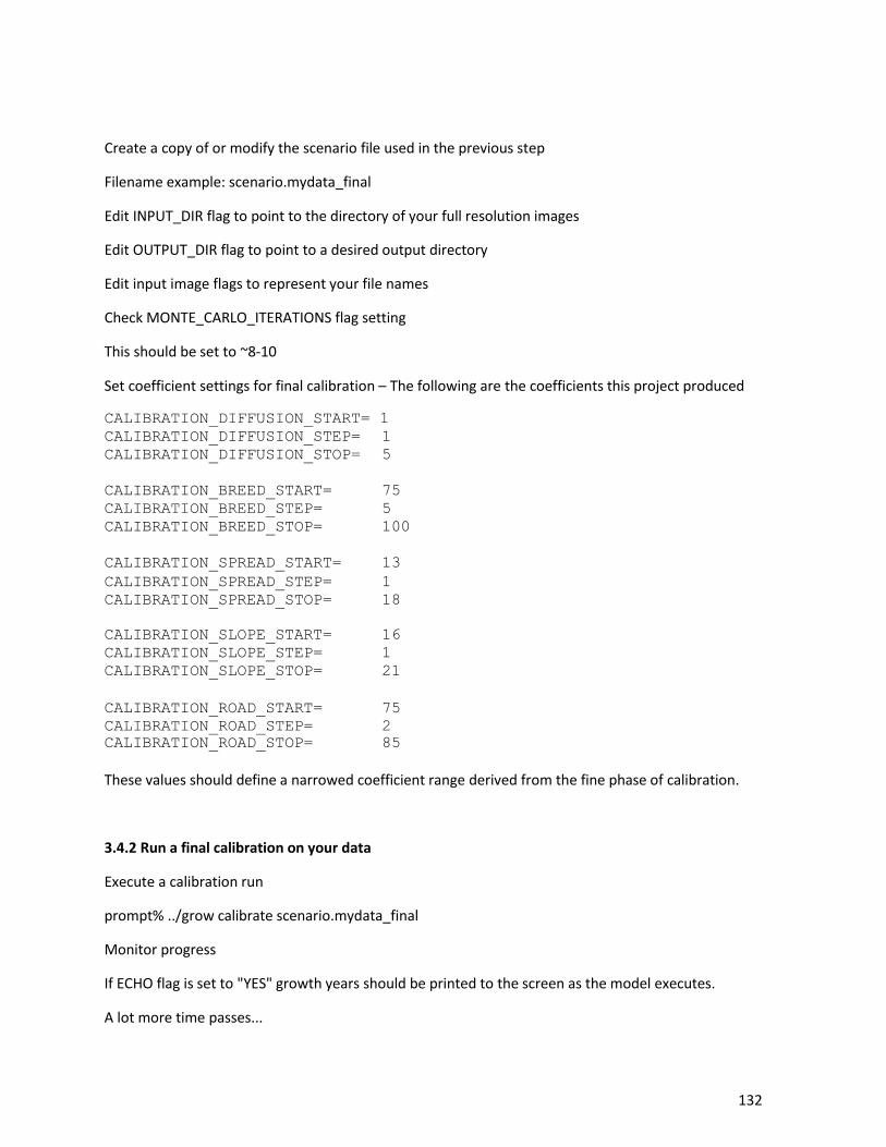
132

Create a copy of or modify the scenario file used in the previous step

Filename example: scenario.mydata_final

Edit INPUT_DIR flag to point to the directory of your full resolution images

Edit OUTPUT_DIR flag to point to a desired output directory

Edit input image flags to represent your file names

Check MONTE_CARLO_ITERATIONS flag setting

This should be set to ~8-10

Set coefficient settings for final calibration – The following are the coefficients this project produced

CALIBRATION_DIFFUSION_START= 1

CALIBRATION_DIFFUSION_STEP= 1

CALIBRATION_DIFFUSION_STOP= 5

CALIBRATION_BREED_START= 75

CALIBRATION_BREED_STEP= 5

CALIBRATION_BREED_STOP= 100

CALIBRATION_SPREAD_START= 13

CALIBRATION_SPREAD_STEP= 1

CALIBRATION_SPREAD_STOP= 18

CALIBRATION_SLOPE_START= 16

CALIBRATION_SLOPE_STEP= 1

CALIBRATION_SLOPE_STOP= 21

CALIBRATION_ROAD_START= 75

CALIBRATION_ROAD_STEP= 2

CALIBRATION_ROAD_STOP= 85

These values should define a narrowed coefficient range derived from the fine phase of calibration.

3.4.2 Run a final calibration on your data

Execute a calibration run

prompt% ../grow calibrate scenario.mydata_final

Monitor progress

If ECHO flag is set to "YES" growth years should be printed to the screen as the model executes.

A lot more time passes...

133

Examine output

The primary file used for coefficient range selection is the control_stats.log file. For more information on how ranges are selected see selecting coefficients.

3.5. Derive forecasting coefficients

The calibration process produces initializing coefficient values that best simulate historical growth for a region. However, due to SLEUTH's self-modification qualities, coefficient values at the START_DATE of a run may be altered by the STOP_DATE. For forecast initialization, the STOP_DATE values from the best calibrated coefficients are desired. Using the best coefficients derived from calibration and running SLEUTH for the historical time period will produce a single set of STOP_DATE coefficients to initialize forecasting. However, due to the random variability of the model, averaged coefficient results of many monte carlo iterations will produce a more robust forecasting coefficient set.

3.4.1. Modify scenario file

Create a copy of or modify the scenario file used in the previous step

Filename example: scenario.mydata

The INPUT_DIR flag should point to the directory of your full resolution images

The OUTPUT_DIR flag should point to a desired output directory

The input image flags should represent your full size file names

Check MONTE_CARLO_ITERATIONS flag setting

This should be set very high (e.g.; 100 or greater))

Set initializing coefficient settings

These values should define a single set of best coefficient values derived from the final phase of calibration. The _START and _STOP values should be equal, and the _STEP value should be one (1).

Set the WRITE_AVG_FILE(YES/NO) flag to "YES"

(The coeff.log file may also be used to find the STOP_DATE coefficient values.)

3.4.2. Find forecasting coefficients

Execute a calibration run

prompt% ../grow calibrate scenario.mydata

134

Monitor progress

If ECHO flag is set to "YES" growth years should be printed to the screen as the model executes.

Examine output

The file used to store coefficient values is the avg.log file. For more information on how to use this file see selecting coefficients.

Step 4: Selecting Coefficient Ranges

The control_stats.log file is the primary file used to score the many runs executed during a calibration phase. By sorting on one or more of the metrics contained in the control_stats.log file, coefficient sets that performed best may be found. Using this information, the user must decide what coefficient ranges will be used for the subsequent phase of calibration.

The algorithm for narrowing these ranges is an area of continuous discussion among users, and so far no definitive "right" way has been agreed upon. Examples of approaches used thus far include: sorting on all metrics equally, weighting some metrics more heavily than others, and sorting only on one metric. Ron Matheny of the Environmental Protection Agency wrote a simple SAS script to sort the control_stats.log file that may be downloaded here. For the sake of clarity in this example, the last method, sorting on one metric, is applied. Simulations are scored on their performance for the spatial match, or lee sallee, metric.

Another disputed issue associated with this process is how many of the best scores should influence the range selection: the top 5, 10, 50? This too is an area that is ripe for more research. The pragmatic answer is enough to capture good results, while substantially reducing the values' spread.

4.1 Selecting coefficients with Optimum SLEUTH Metric (OSM)

Optimum SLEUTH Metric (Dietzel and Clarke, 2007) code is provided in the Download page. After each phase of calibration OSM code can be run using the control_stats.log file to find out the 'top 50' best fit values.

1. Download the OSM code, unzip and place it in the 'Output' directory.

2. Execute the OSM run

prompt% ./readdata2

autoprompt 'Enter the input file name:' % control_stats.log

3. This generates 'top50.txt' which stores the top 50 best fit set of coefficient values.

4. For the top three rankings: take high and low values of each of the coefficients.It is possible for more than one run to have the same score, creating a tie

5. For each coefficient: in the scenario file to be used for fine calibration, low values are set to _START

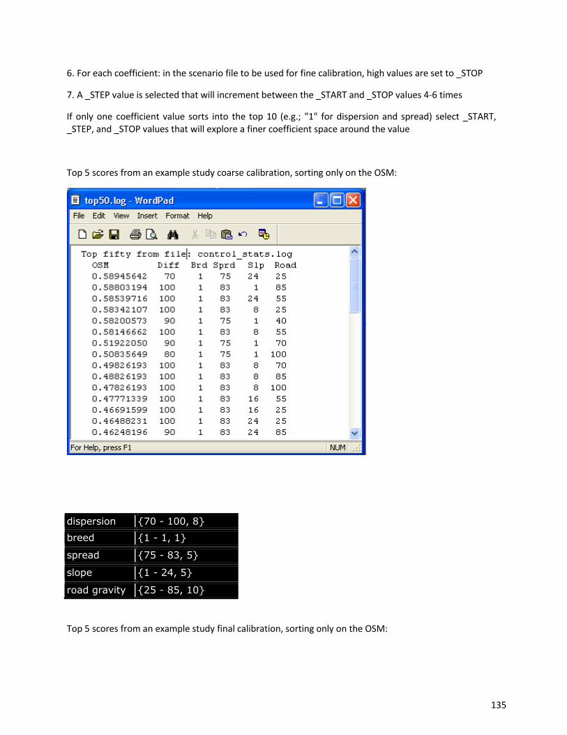
135

6. For each coefficient: in the scenario file to be used for fine calibration, high values are set to _STOP

7. A _STEP value is selected that will increment between the _START and _STOP values 4-6 times

If only one coefficient value sorts into the top 10 (e.g.; "1" for dispersion and spread) select _START, _STEP, and _STOP values that will explore a finer coefficient space around the value

Top 5 scores from an example study coarse calibration, sorting only on the OSM:

dispersion {70 - 100, 8}

breed {1 - 1, 1}

spread {75 - 83, 5}

slope {1 - 24, 5}

road gravity {25 - 85, 10}

Top 5 scores from an example study final calibration, sorting only on the OSM:

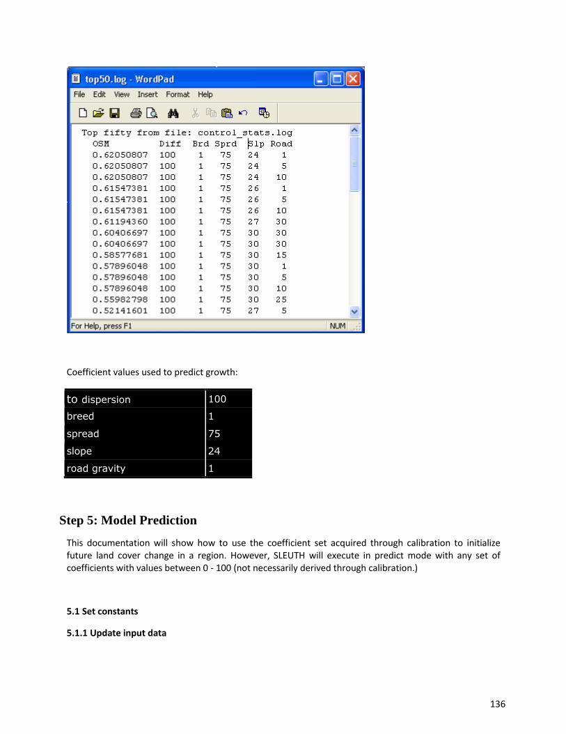
136

Coefficient values used to predict growth:

to dispersion 100

breed 1

spread 75

slope 24

road gravity 1

Step 5: Model Prediction

This documentation will show how to use the coefficient set acquired through calibration to initialize future land cover change in a region. However, SLEUTH will execute in predict mode with any set of coefficients with values between 0 - 100 (not necessarily derived through calibration.)

5.1 Set constants

5.1.1 Update input data

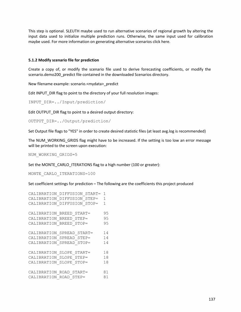
137

This step is optional. SLEUTH maybe used to run alternative scenarios of regional growth by altering the input data used to initialize multiple prediction runs. Otherwise, the same input used for calibration maybe used. For more information on generating alternative scenarios click here.

5.1.2 Modify scenario file for prediction

Create a copy of, or modify the scenario file used to derive forecasting coefficients, or modify the scenario.demo200_predict file contained in the downloaded Scenarios directory.

New filename example: scenario.<mydata>_predict

Edit INPUT_DIR flag to point to the directory of your full resolution images:

INPUT_DIR=../Input/prediction/

Edit OUTPUT_DIR flag to point to a desired output directory:

OUTPUT_DIR=../Output/prediction/

Set Output file flags to "YES" in order to create desired statistic files (at least avg.log is recommended)

The NUM_WORKING_GRIDS flag might have to be increased. If the setting is too low an error message will be printed to the screen upon execution:

NUM_WORKING_GRIDS=5

Set the MONTE_CARLO_ITERATIONS flag to a high number (100 or greater):

MONTE_CARLO_ITERATIONS=100

Set coefficient settings for prediction – The following are the coefficients this project produced CALIBRATION_DIFFUSION_START= 1

CALIBRATION_DIFFUSION_STEP= 1

CALIBRATION_DIFFUSION_STOP= 1

CALIBRATION_BREED_START= 95

CALIBRATION_BREED_STEP= 95

CALIBRATION_BREED_STOP= 95

CALIBRATION_SPREAD_START= 14

CALIBRATION_SPREAD_STEP= 14

CALIBRATION_SPREAD_STOP= 14

CALIBRATION_SLOPE_START= 18

CALIBRATION_SLOPE_STEP= 18

CALIBRATION_SLOPE_STOP= 18

CALIBRATION_ROAD_START= 81

CALIBRATION_ROAD_STEP= 81

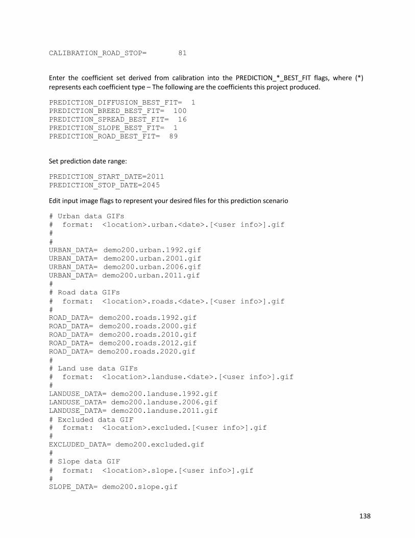
138

CALIBRATION_ROAD_STOP= 81

Enter the coefficient set derived from calibration into the PREDICTION_*_BEST_FIT flags, where (*) represents each coefficient type – The following are the coefficients this project produced.

PREDICTION_DIFFUSION_BEST_FIT= 1

PREDICTION_BREED_BEST_FIT= 100

PREDICTION_SPREAD_BEST_FIT= 16

PREDICTION_SLOPE_BEST_FIT= 1

PREDICTION_ROAD_BEST_FIT= 89

Set prediction date range:

PREDICTION_START_DATE=2011

PREDICTION_STOP_DATE=2045

Edit input image flags to represent your desired files for this prediction scenario

# Urban data GIFs

# format: <location>.urban.<date>.[<user info>].gif

#

#

URBAN_DATA= demo200.urban.1992.gif

URBAN_DATA= demo200.urban.2001.gif

URBAN_DATA= demo200.urban.2006.gif

URBAN_DATA= demo200.urban.2011.gif

#

# Road data GIFs

# format: <location>.roads.<date>.[<user info>].gif

#

ROAD_DATA= demo200.roads.1992.gif

ROAD_DATA= demo200.roads.2000.gif

ROAD_DATA= demo200.roads.2010.gif

ROAD_DATA= demo200.roads.2012.gif

ROAD_DATA= demo200.roads.2020.gif

#

# Land use data GIFs

# format: <location>.landuse.<date>.[<user info>].gif

#

LANDUSE_DATA= demo200.landuse.1992.gif

LANDUSE_DATA= demo200.landuse.2006.gif

LANDUSE_DATA= demo200.landuse.2011.gif

# Excluded data GIF

# format: <location>.excluded.[<user info>].gif

#

EXCLUDED_DATA= demo200.excluded.gif

#

# Slope data GIF

# format: <location>.slope.[<user info>].gif

#

SLOPE_DATA= demo200.slope.gif

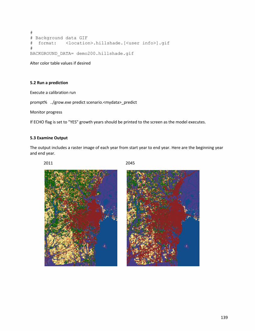
139

#

# Background data GIF

# format: <location>.hillshade.[<user info>].gif

#

BACKGROUND_DATA= demo200.hillshade.gif

Alter color table values if desired

5.2 Run a prediction

Execute a calibration run

prompt% ../grow.exe predict scenario.<mydata>_predict

Monitor progress

If ECHO flag is set to "YES" growth years should be printed to the screen as the model executes.

5.3 Examine Output

The output includes a raster image of each year from start year to end year. Here are the beginning year and end year.

2011 2045

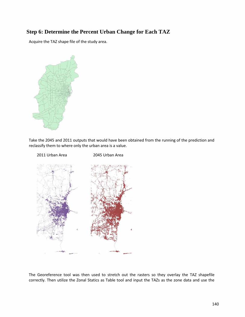
140

Step 6: Determine the Percent Urban Change for Each TAZ

Acquire the TAZ shape file of the study area.

Take the 2045 and 2011 outputs that would have been obtained from the running of the prediction and reclassify them to where only the urban area is a value.

2011 Urban Area 2045 Urban Area

The Georeference tool was then used to stretch out the rasters so they overlay the TAZ shapefile correctly. Then utilize the Zonal Statics as Table tool and input the TAZs as the zone data and use the

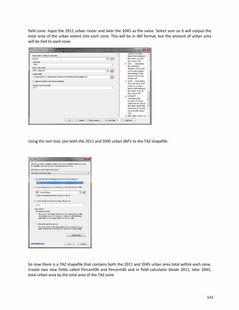
141

field zone. Input the 2011 urban raster and later the 2045 as the value. Select sum so it will output the total area of the urban extent into each zone. This will be in dbf format, but the amount of urban area will be tied to each zone.

Using the Join tool, join both the 2011 and 2045 urban dbf’s to the TAZ shapefile.

So now there is a TAZ shapefile that contains both the 2011 and 2045 urban area total within each zone. Create two new fields called Percent06 and Percent40 and in field calculator divide 2011, later 2045, total urban area by the total area of the TAZ zone.

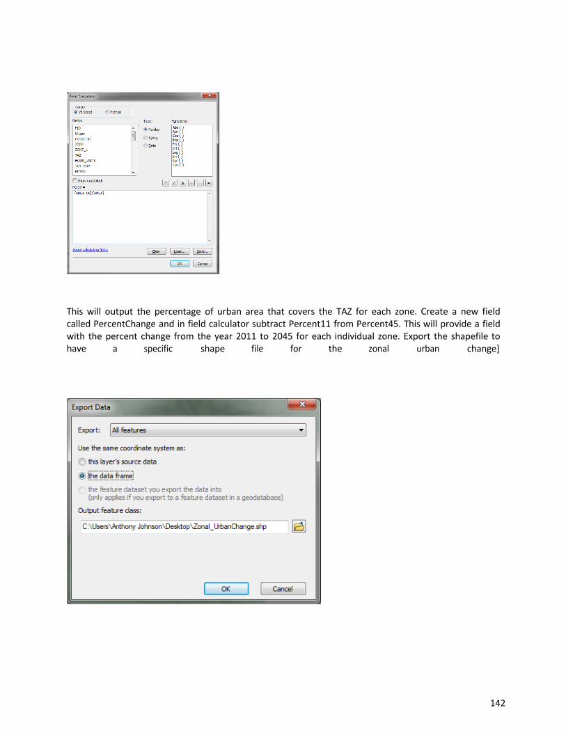
142

This will output the percentage of urban area that covers the TAZ for each zone. Create a new field called PercentChange and in field calculator subtract Percent11 from Percent45. This will provide a field with the percent change from the year 2011 to 2045 for each individual zone. Export the shapefile to have a specific shape file for the zonal urban change]

143

Appendix A12 2015-2045 Volume Plots

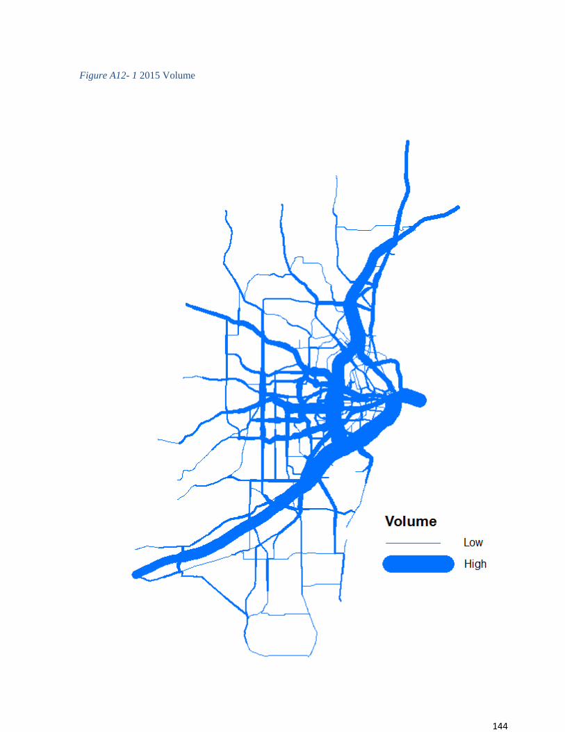
144

Figure A12- 1 2015 Volume

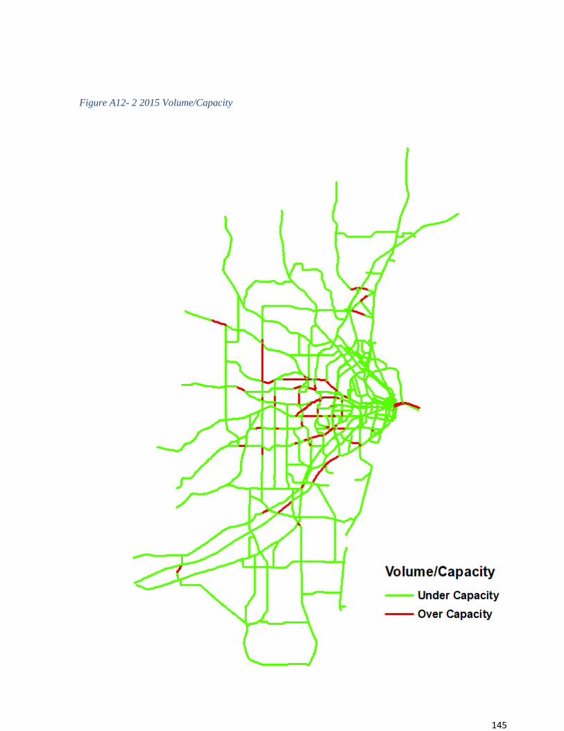
145

Figure A12- 2 2015 Volume/Capacity

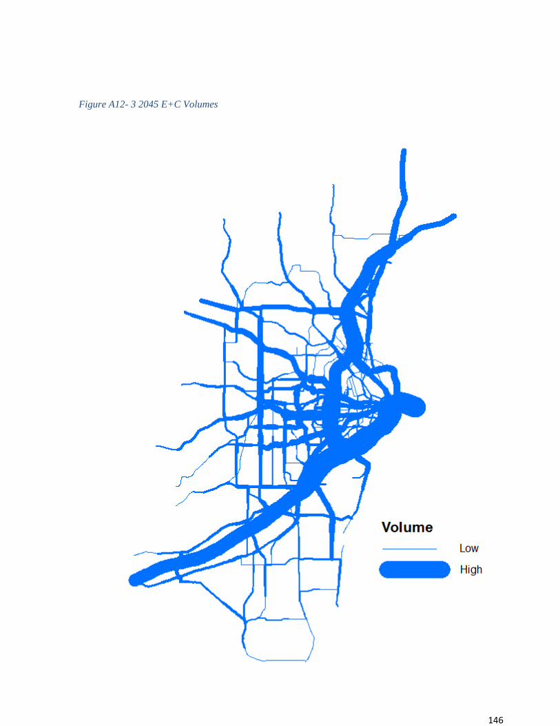
146

Figure A12- 3 2045 E+C Volumes

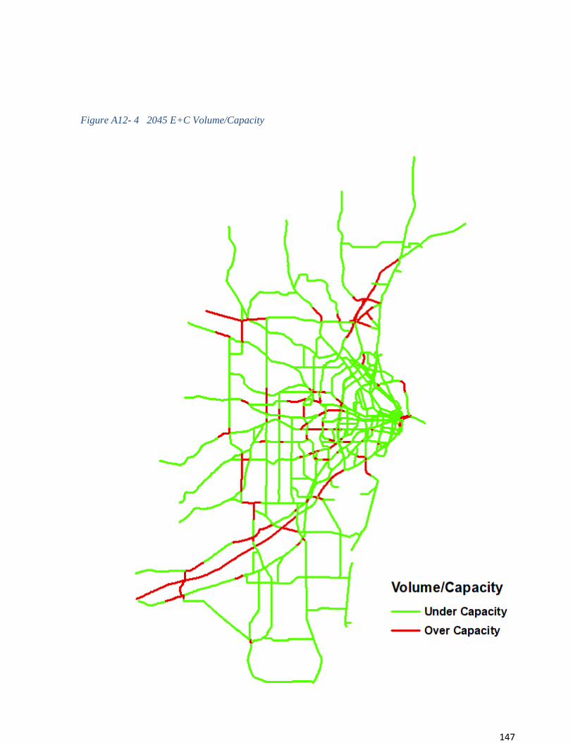
147

Figure A12- 4 2045 E+C Volume/Capacity

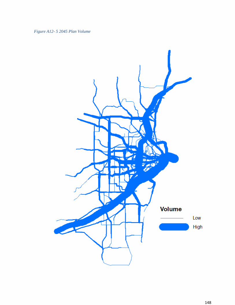
148

Figure A12- 5 2045 Plan Volume

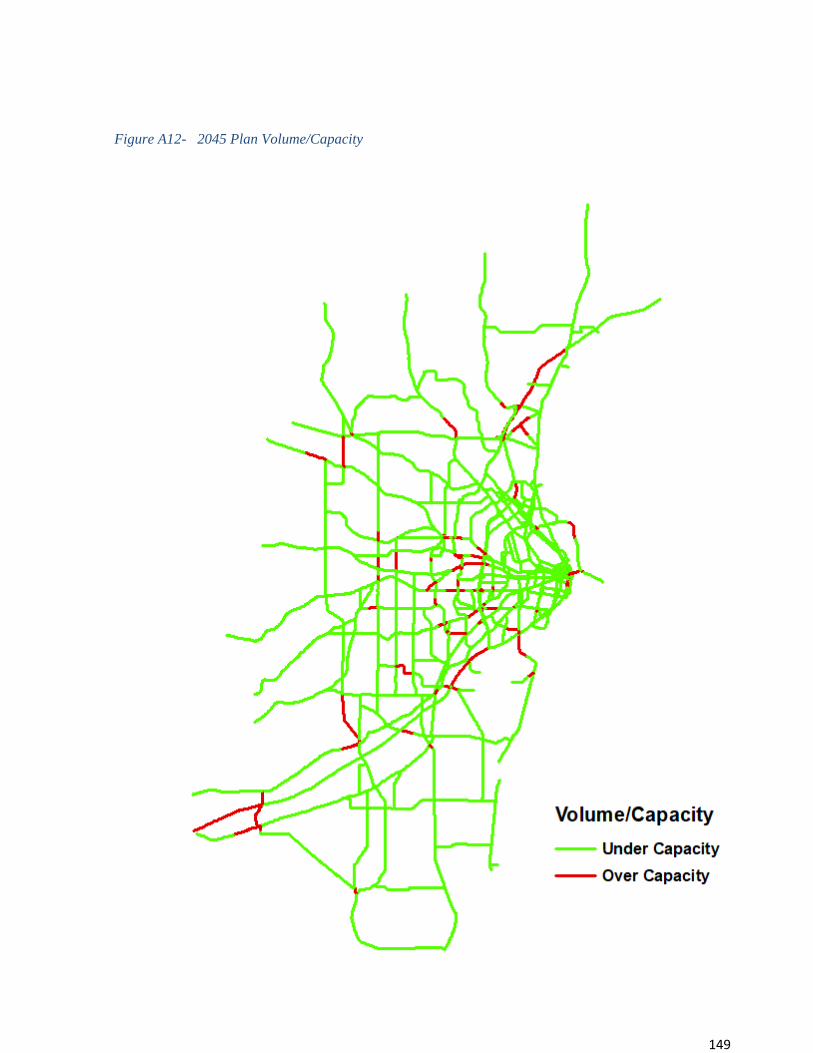
149

Figure A12- 2045 Plan Volume/Capacity