202: Dynamic Macroeconomic Theoryecondse.org/wp-content/uploads/2015/02/C202-OLG-Model.pdf · 202:...

202: Dynamic Macroeconomic TheorySamuelson-Diamond Overlapping Generations Model

Mausumi Das

Lecture Notes, DSE

February 19 & 25-26, 2015

Das (Lecture Notes, DSE) Dynamic Macro February 19 & 25-26, 2015 1 / 33

Samuelson-Diamond Overlapping Generations Model

We have so far analysed optimizing savings behaviour by thehouseholds in the context of the inifinite horizon R-C-K framework.We now turn to an alternative framework, where agents optimize overa finite time horizon.This framework was first developed by Samuelson (1958) in thecontext of an exchange economy, which was later extended to aproduction economy by Peter Diamond (1965).Each agent now lives exactly for T periods. For convenience, we shallassume that T = 2.We shall denote these two periods of an agent’s life time by ‘youth’and ‘old-age’respectively.The agent works only in the first period of his life (when young) andis retired in the second period (when old).Thus he has to make provisions for his old-age consumption from hisfirst period wage income itself (through savings).The agent optimally decides about his consumption profile bymaximizing his life-time utility (to be specified later).


OLG Model: Production Side Story

Once again, the production side story in the OLG model is identicalto that of Solow.Thus the economy starts with a given stock of capital (Kt) and agiven stock of labour force (Nt) at time t.Notice that since people do not work during their oldage, the currentlabour force consist only of the current youth.We also assume that all firms have access to an identical productiontechnology - which satisfies all standard neoclassical properties.The firm-specific production functions can be aggregated to generatean aggregate production function such that :

Yt = F (Kt ,Nt ).

At every point of time the market clearing wage rate and the rentalrate of capital are given by:

wt = FN (Kt ,Nt ); rt = FK (Kt ,Nt ).


OLG Model: Household Side Story

There are H households or dynasties in the economy. In everyhousehold, at any point of time t, there are two cohorts of agents -those who are born in period t (‘generation t’- who are currentlyyoung) and those who were born in the previous period (‘generationt − 1’- who are currently old): hence the name ‘overlappinggenerations’.Thus at any point of time t, total population consists of twosuccessive generations of people:

Lt = Nt +Nt−1.

(Notice that although total population is Lt , total labour force attime t in only Nt .)We shall assume that population in successive generations grows at aconstant rate n :

Nt+1 = (1+ n)Nt .

Hence total population in the economy (Lt) also grows at the sameconstant rate n.


Life Cycle of a Representative Member of Generation t:

All agents within a generation are identical. So we can talk in termsof a representative agent belonging to ‘generation t’.

The agent is born at the beginning of period t with an endowment ofone unit of labour.

All agents in this model are selfish - they care only about their ownconsumption/utility and not about their childrens’utility. Hence theydo not leave any bequest.

No bequest implies that the young agent has only labour endowmentand no capital endowment.

The young agent in period t supplies his labour inelastically to thelabour market in period t to earn a wage income wt .

Out of this wage income, the agent consumes a part and saves therest - which becomes his capital stock in the next period and allowshim to earn a rental income in the next period.


Representative Agent’s Utility Function:

Notice that since the agent would not be working in the next period,the savings and the consequent ownership of capital is the only sourceof income for him in the next period.Thus an agent is a worker in the first period of his life and becomes acapitalist (capital-owner) in the second period of his life.The young agent in period t optimally decides on his currentconsumption (c1t ) and current savings (st) (or equivalently, his currentconsumption (c1t ) and future consumption (c

2t+1)) so as to maximise

his lifetime utility:

U(c1t , c2t+1) ≡ u(c1t ) + βu(c2t+1); 0 < β < 1, (1)

where u′ > 0; u′′ < 0; limc→0

u′(c) = ∞; limc→∞

u′(c) = 0.

β is the standard discount factor, which can be thought of as

β ≡ 11+ ρ

where ρ represents the pure rate of time preference.


Representative Agent’s Budget Constraints:

The first period budget constraint of the agent:

c1t + st = wt .

The second period budget constraint of the agent:

c2t+1 = (1+ ret+1 − δ)st .

Combining, we get the life-time budget constraint of the agent as:

c1t +c2t+1

(1+ r et+1 − δ)= wt . (2)

The agent decides on his optimal consumption in the two periods bymaximising (1) subject to (2).Since the agent is taking his savings decision in the first period, whensecond period’s market interest rate is not yet known, he mustoptimize on the basis of some expected value of the rt+1.As before, we shall assume that agents have perfectforesight/rational expectations such that r et+1 = rt+1 for all t.


Representative Agent’s Optimal Consumption & Savings:

From the FONC of the optimization exercise:

u′(c1t )u′(c2t+1)

= β(1+ rt+1 − δ). (3)

From the FONC and the life-time budget constraint, we can derivethe optimal solutions as:

c1t = ψ(wt , rt+1);

c2t+1 = η(wt , rt+1).

Corresponding optimal savings:

st = wt − ψ(wt , rt+1) ≡ φ(wt , rt+1).

Before we proceed further, it is useful to note the signs of the partialderivatives sw and sr .


Representative Agent’s Optimal Consumption & Savings(Contd.):

Notice that

sw ≡∂φ(wt , rt+1)

∂wt= 1− ∂ψ(wt , rt+1)

∂wt= 1− ∂c1t

∂wt.

From the life-time budget constraint of the agent:

∂c1t∂wt

+1

(1+ rt+1 − δ)

∂c2t+1∂wt

= 1.

Under the assumption that both c1t and c2t_1 are normal goods, a unit

increase in the wage rate wt ceteris paribus must increase both c1t

and c2t+1. Thus 0 <∂c1t∂wt

,∂c2t+1∂wt

< 1.

This in turn implies that

0 < sw < 1.



The sign of sr however is ambiguous.

Notice that

sr ≡∂φ(wt , rt+1)

∂rt+1= −∂ψ(wt , rt+1)

∂rt+1= − ∂c1t

∂rt+1.

So the sign of sr depends on how first period consumption respondsto a unit change in rt+1.

Recall however that1

1+ rt+1 − δis the relative price of c2t+1 in terms

of c1t .

Thus a unit increase in rt+1 ceteris paribus reduces the relative priceof future consumption in terms of current consumption.



Any such price change will be associated with two effects:a substitution effect (⇒ consumption should move in favour of therelatively cheaper good);an income effect (⇒ the budget set of the consumer expands, whichincreases consumption of both goods)

Thus due to an increase in rt+1 ceteris paribusc1t should decrease due to the substitution effect, whilec1t should increase due to the income effect of a price change.

The sign of∂c1t

∂rt+1depends on which effect dominates.

This in turn implies that

sr R 0

according as, substitution effect R income effect.


Aggregate Consumption & Savings:

Let us now turn our attention to the aggregate economy.

Recall that in every period the total output is distributed as wageincome and capital income:

Yt = wtNt + rtKt . (4)

The entire wage income goes to the current young generation. Eachof them saves a part of the wage income (st) and consume the rest.Thus,

wtNt = c1t Nt + stNt .

On the other hand, the entire interest income goes to the current oldgeneration. Each of them consume not only the interest earnings butthe left over capital stock as well. Thus,

c2t Nt−1 = rtKt + (1− δ)Kt .


Aggregate Consumption & Savings (Contd.):

Thus aggregate consumption in this economy at time t :

Ct = c1t Nt + c2t Nt−1

= [wtNt − stNt ] + [rtKt + (1− δ)Kt ]

= wtNt + rtKt − [stNt − (1− δ)Kt ]︸︷︷︸St

(5)

Notice that aggregate savings St has two components:1 The positive savings by the young (stNt );2 The negative savings by the old (−(1− δ)Kt ).

As before, from the demand-supply equality for the aggregateeconomy:

Ct + It = Yt , where It ≡ Kt+1 − (1− δ)Kt⇒ Kt+1 = stNt .


Dynamics of Capital-Labour Ratio:

Since we know that labour force in this economy is growing at therate n, i.e., Nt+1 = (1+ n)Nt , we can derive the dynamic ofcapital-labour ratio (kt) as:

kt+1 =st

(1+ n)=

φ(wt , rt+1)(1+ n)

. (6)

Again, from the production side of the story, we already know that

wt = f (kt )− kt f ′(kt );rt+1 = f ′(kt+1).

Thus we can write (4) as:

kt+1 =φ(wt (kt ), rt+1(kt+1))

(1+ n)= Φ(kt , kt+1). (7)

Equation (7) is the basic dynamic equation of the OLG model, whichimplicitly defines kt+1 as a function of kt . Given k0, we should be ableto trace the evolution of the capital-labour ratio over time.


Existence of a Unique Perfect Foresight path:

Let us look at dynamic equation (7). Notice that it is an ‘implicit’difference equation with kt+1 entering on both sides.

In fact this implicit nature of the function arises precisely due toassumption of perfect foresight. (Verify that with static expectationthe difference equation is explicit and well-defined).

The implicit function on the RHS poses a problem: for every kt do weneceassrily get a unique kt+1 that satisfy the dynamic equation (7)?In other words, for any given initial value of k0, does a uniqueperfect foresight path exist?Notice that uniqueness is important because otherwise the futuretrajectory of the economy will become indeterminate.


Existence of a Unique Perfect Foresight Path (Contd.):

Notice that for any given value of kt ,say k̄, from (7) we shall have aunique solution for kt+1 if and only if the curve representingΦ(k̄ , kt+1) has a unique point of intersection with the 45o line in thepositive quadrant.A suffi cient condition for this to happen is Φ(k̄ , kt+1) is either a flatline or is downward sloping with respect to kt+1, i.e.,

∂Φ(k̄, kt+1)∂kt+1

5 0 for all k̄ ∈ (0,∞).


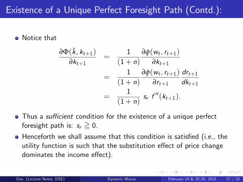
Existence of a Unique Perfect Foresight Path (Contd.):

Notice that

∂Φ(k̄, kt+1)∂kt+1

=1

(1+ n)∂φ(wt , rt+1)

∂kt+1

=1

(1+ n)∂φ(wt , rt+1)

∂rt+1

drt+1dkt+1

=1

(1+ n)sr f ′′(kt+1).

Thus a suffi cient condition for the existence of a unique perfectforesight path is: sr = 0.Henceforth we shall assume that this condition is satisfied (i.e., theutility function is such that the substitution effect of price changedominates the income effect).


Dynamics of Capital-Labour Ratio (Contd.):

Having established that the difference equation given by (7) iswell-defined, let us now characterise the evolution of kt over time.Since Φ(kt , kt+1) is a nonlinear function of kt and kt+1, we shallhave to use the phase diagram technique to qualitatively characterisethe dynamics.In drawing the phase diagram, first note that the slope of the phaseline can be determined by total diffentiating (7):

(1+ n)dkt+1 = swdwtdkt

dkt + srdrt+1dkt+1

dkt+1

i.e.,dkt+1dkt

=sw [−kt f ′′(kt )]

(1+ n)− sr f ′′(kt+1).

Under the assumption that sr = 0, the slope of the phase line isnecessarily positive.But even when the slope is positive, the curvature is not necessarilyconcave - since it would involve the third derivative of the utilityfunction and the f (k) function - whose signs are not known.Hence anything is possible: we may have situations of no steadystate; unique stable steady state; unique unstable steady state;multiple steady states (some stable, some unstable).


Stability & Dynamic Effi ciency in the OLG Model:

In other words, the nice result of the Solow model of a unique andglobally stable steady state is no longer gauranteed - despite theproduction function satifying all the standard neoclassicalproperties - including diminishing returns and the Inadaconditions!What about dynamic effi ciency?

Even that is not gauranteed any more!

Below we provide an example - with specific functional forms - toshow that dynamic effi ciency is not necessarily gauranteed under theOLG model - despite optimizing savings behaviour by the agents.


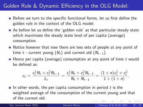
Golden Rule & Dynamic Effi ciency in the OLG Model:

Before we turn to the specific functional forms, let us first define thegolden rule in the context of the OLG model.

As before let us define the ‘golden rule’as that particular steady statewhich maximises the steady state level of per capita (average)consumption.

Notice however that now there are two sets of people at any point oftime t - current young (Nt) and current old (Nt−1).

Hence per capita (average) consumption at any point of time t wouldbe defined as:

ct =c1t Nt + c

2t Nt−1

Lt=c1t Nt + c

2t Nt−1

Nt +Nt−1=(1+ n)c1t + c

2t

1+ (1+ n).

In other words, the per capita consumption in period t is theweighted average of the consumption of the current young and thatof the current old.


Characterization of the Steady State in OLG Model:

So what would be the steady state value of per capita consumption?Recall that the basic dynamic equation is the OLG model is given by:

kt+1 =st

(1+ n)=

φ(w(kt ), r(kt+1))(1+ n)

Accordingly, the steady state(s) of the OLG model is defined as:

k∗ =s∗

(1+ n)=

φ(w(k∗), r(k∗))(1+ n)

⇒ s∗ = (1+ n)k∗ (8)

On the other hand, from the optimal solutions of c1 and c2, we knowthat at steady state:(

c1)∗

= ψ(w(k∗), r(k∗)) = w(k∗)− s∗; (9)(c2)∗

= η(w(k∗), r(k∗)) = [1+ r(k∗)− δ] s∗. (10)


Steady State Per Capita Consumption in the OLG Model:

Hence from (1), (2) & (3) steady state per capita consumption:

c∗ =(1+ n)

(c1)∗+(c2)∗

1+ (1+ n)

=(1+ n) [w(k∗)− s∗] + [(1+ r(k∗)− δ)] s∗

1+ (1+ n)

=(1+ n)w(k∗) + [r(k∗)− δ− n)] s∗

1+ (1+ n)

=(1+ n) [{w(k∗) + r(k∗)k∗} − (n+ δ)k∗]

1+ (1+ n)

=1+ n

1+ (1+ n)[f (k∗)− (n+ δ)k∗] .

Maximizing c∗ with respect to k∗, we would still get the golden rulecondition as:

kg : f ′(k∗) = (n+ δ)


Alternative Definition of Golden Rule:

An alternative definition of the ‘golden rule’in the context of theOLG model can be as follows: it is that particular steady state whichmaximises the steady state level of utility of any agent.When the economy is at a steady state both w and r becomeconstants. Thus for any agent belonging to any generation (t − 1 or tor t + 1), the life-time consumption profile look exactly the same:

c1t−1 = c1t = c1t+1 = ψ(w(k∗), r(k∗)) ≡

(c1)∗;

c2t = c2t+1 = c2t+2 = η(w(k∗), r(k∗)) ≡

(c2)∗.

Hence steady state utility of any generation is given by:

U((c1)∗,(c2)∗) ≡ u(

(c1)∗) + βu(

(c2)∗).

It is easy to check that the k∗ that maximises U((c1)∗,(c2)∗) is still

given by:kg : f ′(k∗) = (n+ δ).

Thus the two definitions of the golden rule are equivalent. (Verify.)Das (Lecture Notes, DSE) Dynamic Macro February 19 & 25-26, 2015 23 / 33

OLG Model with Specific Functional Forms:

Let us now assume specific functional forms.

LetU(c1t , c

2t+1) ≡ log c1t + β log c2t+1;

f (kt ) = (kt )α ; 0 < α < 1.

Also let the rate of depreciation be 100%, i.e., δ = 1.

Thus the life-time budget constraint of the representative agent ofgeneration t is given by:

c1t +c2t+1rt+1

= wt .

The corresponding FONC:

c2t+1c1t

= βrt+1. (11)


OLG Model: Specific Functional Forms (Contd.)

From the FONC and the life-time budget constraint, we can derivethe optimal solutions as:

c1t =1

1+ βwt ;

st =β

1+ βwt ;

c2t+1 = βrt+1

[1

1+ βwt

].

Corresponding dynamic equation:

kt+1 =st

(1+ n)=

(1

1+ n

) [β

1+ βwt

].

Finally, given the production function,

wt = (1− α) (kt )α


OLG Model: Dynamics with Specific Functional Forms

Thus the dynamics of this specific case is simple:

kt+1 =(

11+ n

)(β

1+ β

)(1− α) (kt )

α .

It is easy to see that the above phase line will generate a uniquenon-trivial steady state which is globally stable.

The corresponding steady state solution is defined as:

k∗ =

(1

1+ n

)(β

1+ β

)(1− α) (k∗)α

i.e., k∗ =

[(1

1+ n

)(β

1+ β

)(1− α)

] 11−α

.

Is this steady state dynamically effi cient? Not necessarily!


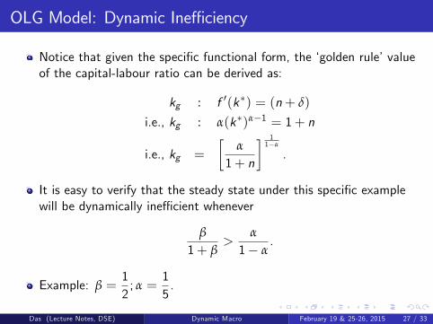
OLG Model: Dynamic Ineffi ciency

Notice that given the specific functional form, the ‘golden rule’valueof the capital-labour ratio can be derived as:

kg : f ′(k∗) = (n+ δ)

i.e., kg : α(k∗)α−1 = 1+ n

i.e., kg =

[α

1+ n

] 11−α

.

It is easy to verify that the steady state under this specific examplewill be dynamically ineffi cient whenever

β

1+ β>

α

1− α.

Example: β =12; α =

15.


Reason for Dynamic Ineffi ciency in the OLG Model:

Thus we see that dynamic ineffi ciency may arise in the OLG model -despite optimizing savings behaviour by households.

This apparently paradoxical result stems from the fact that agents are‘selfish’in the OLG model; they do not care for their children’sutility/consumption.

Thus when they optimise they equate the MRS with (the discountedvalue of) the actual future return (rt+1 + 1− δ):

u′(c1t )u′(c2t+1)

= β(rt+1 + 1− δ).

Now notice that

u′ (ct )u′ (ct+1)

T 1⇒ u′ (ct ) T u′ (ct+1)⇒ ct S ct+1.


Reason for Dynamic Ineffi ciency in OLG Model (Contd.)

This implies that in the OLG framework, ct S ct+1 i.e, consumptionwould rise, fall or remain unchanged over time if the corresponding(future) return, measured by (rt+1 + 1− δ) is greater, equal to or less

than the subjective cost1β≡ (1+ ρ), ie. according as

rt+1 − δ R ρ.

Recall that in the R-C-K model the corresponding equation was givenby:

dcdt=

ctσ(ct )

[rt − δ− n− ρ] .

Thus in the R-C-K framework,dcdtR 0 i.e, consumption would rise,

fall or remain unchanged over time if the correspondingpopulation-adjusted (future) return, measured by (rt − δ− n) isgreater, equal to or less than the subjective cost measured by ρ.


Reason for Dynamic Ineffi ciency in OLG Model (Contd.)

Notice that both in the OLG model and the R-C-K model, householdswill stop saving whenever their percieved return is less than thesubjective cost ρ.But due to presence of intergenerational altrauism, in the R-C-Kmodel the percieved return is adjusted for popultion growth and isgiven by r − δ− n, whereas in the OLG model this return is just r − δ

This implies that in the R-C-K model households will necessarily stopsaving when the (net) marginal product has fallen below thepopulation growth rate (rt − δ− n < 0).But there is no reason why in the OLG model, households would stopsaving in this scenario, because even though the net gross marginalproduct (rt+1 − δ) has fallen below n - it might still greater than thesubjective cost ρ.

Thus there is a tendency to oversave (compared to the R-C-K model),which persists even when the economy has moved into a dynamicallyineffi cient region (i.e., rt+1 < δ+ n ).


Dynamic Ineffi ciency & Scope for Government Interventionin the OLG Model:

Since under the OLG framework, the steady state of the decentralizedmarket economy may be dynamically ineffi cient (despite rationalexpectations on part of the agents), this again justifies a role ofgovernment in improving effi ciency.

Thus the conclusions of the OLG model are diametrically opposite ofthat of the R-C-K model - even though both are based on strictlyneoclassical production function and optimizing agents.

The difference arises primarily due to the absence of parental altruismin the OLG framework.

It can be shown that if we introduce parental altruism in the OLGmodel (by incorporating a bequest term that each parent leaves to hischild at the end of his life time), then the OLG framework will be verysimilar to the R-C-K framework.


OLG Model: Summary

Even though the production function is Neoclassical in the OLGmodel, the strong stability result of Solow (as well as R-C-K model)does not hold:

a steady state may not exists;even if it exists it may not be unique;even if it is unique, it may not be stable.

So the growth conclusions of the Solow model do not hold either.

Moreover the dynamic ineffi ciency problem may reappear here- eventhough each agent is optimally determining his savings behaviour.

Thus in this model there is scope for government intervention interms of improving effi ciency.

Since the OLG model does not obey the growth properties of theSolow/R-C-K model, we do not identify this structure with the“Neoclassical Growth Model" (even though the production structurehere is identical to Solow/R-C-K).


References:

Reference for the OLG Model:

D. Acemoglu: Introduction to Modern Economic Growth, Chapter 9,Sections 9.2,9.3, 9.4 (Pages 329-339).O.Galor & H. Ryder (1989): "Existence, uniqueness, and stability ofequilibrium in an overlapping-generations model with productivecapital,", Journal of Economic Theory, pp.360—375.


202: Dynamic Macroeconomic Theoryecondse.org/wp-content/uploads/2015/02/C202-OLG-Model.pdf · 202:...

Documents

Transcript of 202: Dynamic Macroeconomic Theoryecondse.org/wp-content/uploads/2015/02/C202-OLG-Model.pdf · 202:...