Contentspress.utp.edu.my/wp-content/uploads/2019/07/Platform-Vol... · 2019-07-04 · Abdul Ghani...
48
ISSN 1511-6794 Contents © 2016 Universiti Teknologi PETRONAS PLATFORM January - June 2016 Patron: Y.Bhg. Datuk Ir (Dr) Abdul Rahim B Hashim Advisor: Prof Ir Dr Ahmad Fadzil M Hani PLATFORM Editorial Editor-in-Chief: Assoc. Prof. Dr Mohd Fadzil Hassan Secretariat: UTP Press UTP Publication Committee: Chairman: Prof Ir Dr Ahmad Fadzil M Hani Members: MOR Directors Head of Departments Secretary: Naziri Yusof Layout and Production: Mohamed Azaman Ismail UTP Press Address: PLATFORM Editor-in-Chief Universiti Teknologi PETRONAS 32610 Seri Iskandar, Perak Darul Ridzuan, Malaysia http://www.utp.edu.my [email protected] [email protected] Telephone +(60)5 368 8687 Facsimile +(60)5 365 4090 Published by UTP Press Universiti Teknologi PETRONAS, Owned by Institute of Technology PETRONAS Sdn Bhd. 2016 Geomechanical Characterisation of the Lumut Granite, Perak, Malaysia Abdul Ghani Md Rafek, Hanif Mohamad 2 Management Model of Plant Turnaround Maintenance for Malaysian Petrochemical Companies Zulkipli Ghazali 10 Elastic Properties and Seismic Attributes Study of Soft Shale and Gas Sand in Sabah Basin Adelynna Shirley anak Penguang, Luluan Almanna Lubis, Deva Prasad Ghosh 20 Reviewers 48 Copyright and Reprint Permission All rights reserved. No part of this publication may be reproduced or transmitted in any form or by any means, including photocopying and recording, without the written permission of the copyright holder, application for which should be addressed to the publisher. Such written permission must also be obtained before any part of this publication is stored in a retrieval system of any nature. The publisher, authors, contributors and endorsers of this publication each excludes liability for loss suffered by any person resulting in any way from the use of, or reliance on this publication.
Transcript of Contentspress.utp.edu.my/wp-content/uploads/2019/07/Platform-Vol... · 2019-07-04 · Abdul Ghani...

I S S N 1 5 1 1 - 6 7 9 4
Contents
© 2016Universiti Teknologi PETRONAS
PLATFORMJanuary - June 2016
Patron:Y.Bhg. Datuk Ir (Dr) Abdul Rahim B Hashim
Advisor: Prof Ir Dr Ahmad Fadzil M Hani
PLATFORM Editorial
Editor-in-Chief:Assoc. Prof. Dr Mohd Fadzil Hassan
Secretariat:UTP Press
UTP Publication Committee:
Chairman: Prof Ir Dr Ahmad Fadzil M Hani
Members:MOR DirectorsHead of Departments
Secretary:Naziri Yusof
Layout and Production:
Mohamed Azaman IsmailUTP Press
Address:PLATFORM Editor-in-ChiefUniversiti Teknologi PETRONAS32610 Seri Iskandar, Perak Darul Ridzuan, Malaysia
http://www.utp.edu.my
[email protected]@utp.edu.my
Telephone +(60)5 368 8687
Facsimile +(60)5 365 4090
Published byUTP PressUniversiti Teknologi PETRONAS,Owned by Institute of Technology PETRONAS Sdn Bhd.2016
Geomechanical Characterisation of the Lumut Granite, Perak, Malaysia
Abdul Ghani Md Rafek, Hanif Mohamad 2
Management Model of Plant Turnaround Maintenance for Malaysian Petrochemical Companies
Zulkipli Ghazali 10
Elastic Properties and Seismic Attributes Study of Soft Shale and Gas Sand in Sabah Basin
Adelynna Shirley anak Penguang, Luluan Almanna Lubis, Deva Prasad Ghosh
20
Reviewers 48
Copyright and Reprint PermissionAll rights reserved. No part of this publication may be reproduced or transmitted in any form or by any means, including photocopying and recording, without the written permission of the copyright holder, application for which should be addressed to the publisher. Such written permission must also be obtained before any part of this publication is stored in a retrieval system of any nature.
The publisher, authors, contributors and endorsers of this publication each excludes liability for loss suffered by any person resulting in any way from the use of, or reliance on this publication.

2 PLATFORM VOLUME TWELVE NUMBER ONE JANUARY - JUNE 2016
PLATFORM - A Journal of Engineering, Science and Society
INTRODUCTION
Lumut is located at the west coast of Perak, about 55 km from Universiti Teknologi PETRONAS. Being the gateway to the resort island of Pangkor as well as a naval base for the Royal Malaysian Navy, this area is undergoing considerable infrastructural development. Since low lying flat areas are limited, this development is now encroaching into the hilly terrain. This hilly terrain consists of a number of granite hills, the highest being Bt. Ungku Busu with an elevation of 331 m. Several high and steep road cuts along major roads are also present in this vicinity.
The general geology of the Lumut area has only been described as part of several regional studies, e.g. by Wong [1] and Suntharalingam [2],[3]. The geomechanical characteristics of the Lumut granite have also not been described previously. Taking these factors into consideration, geological mapping together with geomechanical investigations were conducted in the Lumut area. The pertinent findings of this study are presented here.
METHODOLOGY
Geological mapping involved traversing the study area, determining the locations of different geological features and transferring this information onto a topographic map. In the course of geological mapping, sites for geomechanical investigations were also identified.
For the geomechanical investigations, the granite rock mass is classified according to Bieniawski’s [4] Rock Mass Rating Classification. For this purpose, detailed geological discontinuity surveys were conducted and rock samples were collected for laboratory testing. The five basic parameters of the RMR system, i.e. rock material strength, rock quality designation, RQD, discontinuity spacing, condition of discontinuities and groundwater conditions were employed to determine the RMRbasic values for each of the sites. The specific values of each parameter for the five Rock Mass Classes are presented in Table 1.
GEOMECHANICAL CHARACTERISATION OF THE LUMUT GRANITE, PERAK, MALAYSIA
Abdul Ghani Md Rafek, Hanif Mohamad Faculty of Geosciences & Petroleum Engineering,
Universiti Teknologi PETRONAS
Email: [email protected]
ABSTRACT
Geological mapping and geomechanical surveys conducted in Lumut showed that the Lumut granite can be classified as “very good rock” based on Bieniawski’s Rock Mass Rating. The granite has a rock mass cohesion value of > 400 kPa and a friction angle of > 45°. Detailed geological discontinuity surveys carried out showed that the westward dipping slopes in the northern hill have potential plane failure whilst the southwesterly dipping slopes have potential wedge failure. As for the southern hill, southeasterly dipping slopes would have potential plane failure. Distinct differences in the discontinuity distribution patterns in the two hills is an evidence for the existence of a major fault between the two hills. The failure potential of the different slopes should be taken into consideration for infrastructure development.
Keywords: Rock Mass Rating, very good rock, plane failure and wedge failure, fault zone mapping

3VOLUME TWELVE NUMBER ONE JANUARY - JUNE 2016 PLATFORM
PLATFORM - A Journal of Engineering, Science and Society
Table 1 Bieniawski’s Rock Mass Rating Classification
Parameter Ranges of Values
UCSValues >250 Mpa 100 - 200 MPa 50 - 100 MPa 25 - 50 MPa 5 - 25 1 - 5 <1
MPa
Rating 15 12 7 4 2 1 0
RQDValues 90 - 100% 75 - 90% 50 - 75% 25 - 50% 25%
Rating 20 17 13 8 3
Joint SpacingValues > 2 m 0.6 - 2.0 m 200 - 600 mm 60 - 200 mm <60 mm
Rating 20 15 10 8 5
Joint Condition
Values
Very rough surfaces
No Continuous
No separation Unweathered
wall
Slightly rough surfaces
Separation < 1mm
Slightly weathered wall
Slightly rough surfaces
Separation < 1mm
Highly weathered wall
Slickensided surfaces
OR gauge < 5mm thick OR
separation 1-5 mm
Soft gauge > 5 mmOR
separation >5 mmcontinous
Rating 30 25 25 25 0
GroundwaterValues Completely
dry Damp Wet Dripping Flowing
Rating 15 10 7 4 0
Rock mass classes determined from total ratings
Rating 100 - 81 80 - 61 60 - 41 40 - 21 < 20
Class I II III IV V
Description Very good rock Good rock Fair rock Poor rock Very poor rock
RESULTS AND DISCUSSION
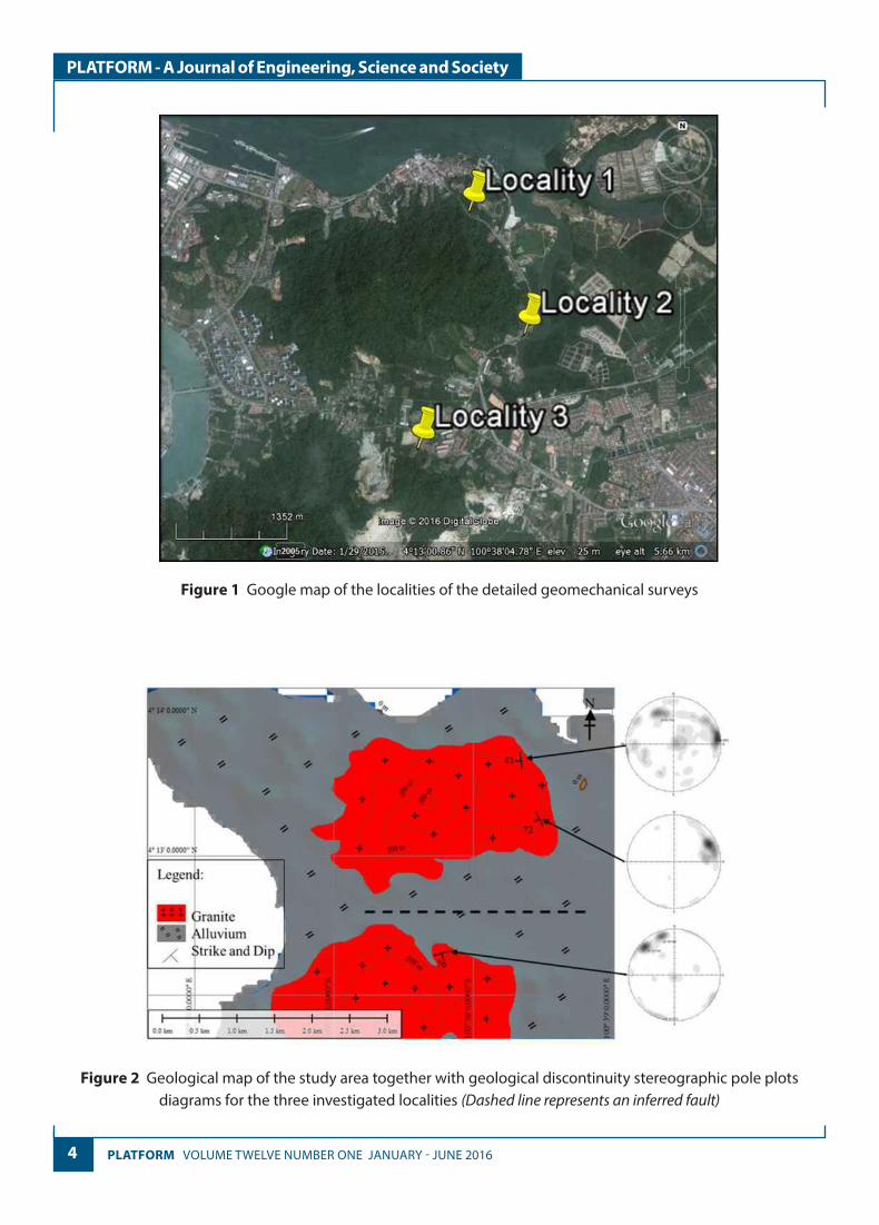
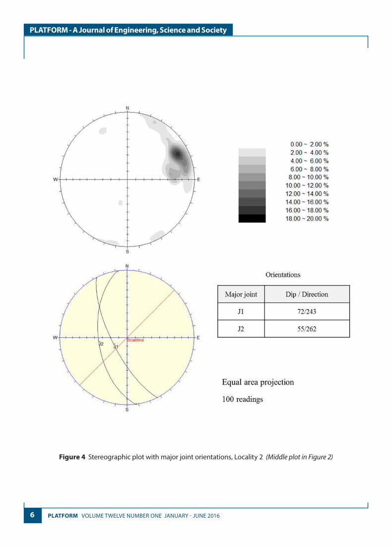
The localities of the detailed geomechanical surveys are shown in Figure 1. The geological map of the study area is shown in Figure 2, together with the stereographic pole plots of the geological discontinuities for the three sites for detailed geomechanical investigation. Figures 3, 4 and 5 show the detailed stereographic plots and major joint orientations for each of the investigated localities. As can be seen in this map, the granite hills are surrounded by unconsolidated alluvium. The stereographic pole plots reveal that the orientation of the major
geological discontinuities at locality one and two, the northern hill are similar, whereas for locality three, the southern hill the orientation is different. This finding provides additional evidence and lends support to the study by Raj [5] of the possible existence of a major fault in the Lumut area. Raj [5] had postulated the existence of this fault based on the analysis of negative lineaments using LANDSAT imagery. Large changes in the orientation of major geological discontinuities within a rock mass provide evidence of the existence of a fault as indicated in Figure 2.
4 PLATFORM VOLUME TWELVE NUMBER ONE JANUARY - JUNE 2016
PLATFORM - A Journal of Engineering, Science and Society
Figure 1 Google map of the localities of the detailed geomechanical surveys
Figure 2 Geological map of the study area together with geological discontinuity stereographic pole plots diagrams for the three investigated localities (Dashed line represents an inferred fault)

5VOLUME TWELVE NUMBER ONE JANUARY - JUNE 2016 PLATFORM
PLATFORM - A Journal of Engineering, Science and Society
Figure 3 Stereographic plot with major joint orientations, Locality 1 (Top plot in Figure 2)
6 PLATFORM VOLUME TWELVE NUMBER ONE JANUARY - JUNE 2016
PLATFORM - A Journal of Engineering, Science and Society
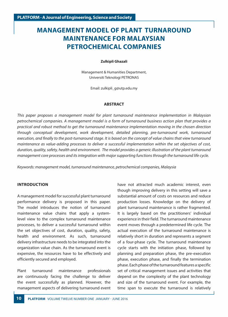
Figure 4 Stereographic plot with major joint orientations, Locality 2 (Middle plot in Figure 2)

7VOLUME TWELVE NUMBER ONE JANUARY - JUNE 2016 PLATFORM
PLATFORM - A Journal of Engineering, Science and Society
Figure 5 Stereographic plot with major joint orientations, Locality 3 (Bottom plot in Figure 2)

8 PLATFORM VOLUME TWELVE NUMBER ONE JANUARY - JUNE 2016
PLATFORM - A Journal of Engineering, Science and Society
Geomechanical investigations at the three sites showed that their Rock Mass Rating, (RMRbasic) exceeded 81. Therefore the granite rock mass for the Lumut area can be classified as “very good rock” with an estimated rock mass cohesion of > 400 kPa and friction angle > 45°.
Results of the discontinuity surveys can be summarized as follows:
i. For the northern granite hill, cut slopes dipping to the west and south west have failure potential. Considering the standard cut rock slope angle of 77° of Jabatan Kerja Raya, westward dipping slope have potential plane failures and slopes dipping to the south west have potential wedge failures.
ii. For the southern granite hill, slopes that dip to the south east have plane failure potential.
CONCLUSION
The geomechanical investigations revealed that the granite in the Lumut area can be classified as “very good rock” with an estimated cohesion of > 400 kPa and a friction angle of > 45°.
Geological discontinuity studies revealed that westward dipping slopes in the northern hill have potential plane failure whilst the southwest dipping slopes are faced with potential wedge failures. For the southern hill, southeast dipping slopes have potential plane failure. This determination of failure potential represents an important input for infrastructure planning.
The distinct differences in the geological discontinuity distribution between the northern hill and southern hill provided additional evidence for the existence of a fault zone between these two hills.
REFERENCES
[1] T.W. Wong, Geology and Mineral Resources of the Lumut-Teluk Intan Area, Perak Darul Ridzuan, Kuala Lumpur: Geological Survey of Malaysia, 1991.
[2] T. Suntharalingam,“Cenozoic Stratigraphy of Peninsular Malaysia”, in Proceeding of The Workshop on Stratigraphic Correlation of Thailand and Malaysia,Vol 1, pp. 149_156,1983.
[3] T. Suntharalingam, “Quaternary stratigraphy and prospects for placer tin in the Taiping-Lumut area, Perak” in Geological Society of Malaysia Bulletin, 17, pp. 9_32, December 1984.
[4] Z.T. Bieniawski, Engineering Rock Mass Classi�cations,New York: Wiley, 1989.
[5] J.K. Raj, “Negative lineaments in granite bedrock areas of NW Peninsular Malaysia”, in Geological Society of Malaysia Bulletin, 16, pp. 61_70, December, 1983.

9VOLUME TWELVE NUMBER ONE JANUARY - JUNE 2016 PLATFORM
PLATFORM - A Journal of Engineering, Science and Society
AUTHORS' INFORMATION
Dr. Abdul Ghani Md Rafek is a professor at the Department of Geosciences, Universiti Teknologi PETRONAS. He joined UTP in 2014 and has over 30 years of research and teaching experience in geomechanics. Prior to joining UTP, he worked at
Universiti Kebangsaan Malaysia. His main research interest is rock mass characterisation and quanti�cation with particular emphasis on geological discontinuity characterisation.
Hanif bin Mohamad completed his degree in Petroleum Geosciences at the Department of Geosciences of UTP. After completing his degree, he joined GeoMag Engineering as an engineering geologist.
10 PLATFORM VOLUME TWELVE NUMBER ONE JANUARY - JUNE 2016
PLATFORM - A Journal of Engineering, Science and Society
MANAGEMENT MODEL OF PLANT TURNAROUND MAINTENANCE FOR MALAYSIAN
PETROCHEMICAL COMPANIES
Zulkipli Ghazali
Management & Humanities Department,Universiti Teknologi PETRONAS
Email: [email protected]
ABSTRACT
This paper proposes a management model for plant turnaround maintenance implementation in Malaysian petrochemical companies. A management model is a form of turnaround business action plan that provides a practical and robust method to get the turnaround maintenance implementation moving in the chosen direction through conceptual development, work development, detailed planning, pre-turnaround work, turnaround execution, and �nally to the post-turnaround stage. It is based on the concept of value chains that view turnaround maintenance as value-adding processes to deliver a successful implementation within the set objectives of cost, duration, quality, safety, health and environment. The model provides a generic illustration of the plant turnaround management core processes and its integration with major supporting functions through the turnaround life cycle.
Keywords: management model, turnaround maintenance, petrochemical companies, Malaysia
INTRODUCTION
A management model for successful plant turnaround performance delivery is proposed in this paper. The model introduces the notion of turnaround maintenance value chains that apply a system-level view to the complex turnaround maintenance processes, to deliver a successful turnaround within the set objectives of cost, duration, quality, safety, health and environment. As such, turnaround delivery infrastructure needs to be integrated into the organization value chain. As the turnaround event is expensive, the resources have to be effectively and efficiently secured and employed.
Plant turnaround maintenance professionals are continuously facing the challenge to deliver the event successfully as planned. However, the management aspects of delivering turnaround event
have not attracted much academic interest, even though improving delivery in this setting will save a substantial amount of costs on resources and reduce production losses. Knowledge on the delivery of plant turnaround maintenance is rather fragmented. It is largely based on the practitioners’ individual experience in their field. The turnaround maintenance event moves through a predetermined life cycle. The actual execution of the turnaround maintenance is relatively short in duration and represents a segment of a four-phase cycle. The turnaround maintenance cycle starts with the initiation phase, followed by planning and preparation phase, the pre-execution phase, execution phase, and finally the termination phase. Each phase of the turnaround features a specific set of critical management issues and activities that depend on the complexity of the plant technology and size of the turnaround event. For example, the time span to execute the turnaround is relatively
11VOLUME TWELVE NUMBER ONE JANUARY - JUNE 2016 PLATFORM
PLATFORM - A Journal of Engineering, Science and Society
short, but it comprises the highest level of activities in the turnaround maintenance cycle. Execution phase is featured by the performance of voluminous tasks by a large number of specialists and tradesmen from various engineering disciplines. In this respect, control and coordination of the workforce and work activities are crucial.
As identified by DeBakey [1], well-established management and organization of the turnaround bring about the high level of certainty and control to the turnaround maintenance event in meeting the budgeted costs, cycle time, quality targets, and safety targets. In view of the above, it is of paramount importance that management of the event is accorded the necessary priority for the event.
PROBLEM STATEMENT
The management of plant turnaround is a scarcely understood and explored subject in management circles. Notwithstanding the extensive body of research on management in the manufacturing and services environment, very limited studies are available on the management of turnaround maintenance. The situation is even more acute when one observes the stark contrast of the mushrooming of plants in the Malaysian petrochemical sector notably in the past four decades. Indeed, numerous studies in practically all aspects of management and business both by local and foreign scholars have failed to attract management of turnaround maintenance as a topic worthy of research inquiry. In comparison to the accrued knowledge on turnaround maintenance from the engineering perspective, rather limited knowledge is available with respect to the organization of one of the most important and critical activities in plant management. As put forth by Gondolfo and Vichich [2], “the management necessary, both in terms of numbers of resources and the composition of players for high complexity turnaround is typically not well understood”. The statement from the two professionals of plant turnaround maintenance in the petrochemical industry in the United States implies the pressing need to address the gap in the
knowledge and the vast opportunity for research and studies on management of turnaround maintenance.
The concerns of many practitioners in the petrochemicals industries in the United States pertaining to the organizational performance of their turnaround maintenance was highlighted by [1], [2] [3], [4] and [5]. Based on their studies, they observed that by and large, turnaround maintenance events experienced 35 percent schedule slippage, 25 percent cost overrun, 40 percent labor-hour growth, and approximately 10 percent scope growth. The highly competitive business environment has further raised the degree and level of interest. This is due to the direct relationship that can be drawn between the profitability of the company and the successful implementation of its plant turnaround maintenance. In the oil and gas industries in the United States, for instance, [2], [3], [4] observed that the high performing companies have been able to manage and organize their turnaround event successfully by establishing effective management system, robust work processes, measurement system that keeps processes in control, organizational memory, and adequate organizational structure. It is not an overstatement to put at the outset that management is one of the factors that influence the turnaround maintenance performance. However, there is no management model on best practices developed specifically for turnaround maintenance management. Industry practitioners who are interested in implementing best practices to better their plant turnaround maintenance events would benefit from this model. Hence, a model for successful plant turnaround performance management is proposed in this paper.
OBJECTIVE
The aim of this study is to develop a generic model for managing plant turnaround maintenance of petrochemicals companies in Malaysia. Central to this model is the diagrammatic representation of the key and support management functions and processes. The model provides a broad perspective of managing the turnaround maintenance throughout its lifecycle.
12 PLATFORM VOLUME TWELVE NUMBER ONE JANUARY - JUNE 2016
PLATFORM - A Journal of Engineering, Science and Society
1. To carry out a comparative analysis of the various primary and support activities of plant turnaround maintenance across various petrochemical companies in Malaysia.
2. To ascertain the connection between all these activities for successful completion of the turnaround event.
3. To create management model for plant turnaround for application in Malaysian petrochemical companies.
METHODOLOGY
The study is carried out in two stages. Initially, review of the literature on practices for turnaround planning and management were done. It provides a background of management practices implemented by petrochemical plants. List of primary activities along the phases of the plant turnaround maintenance was identified. Various associated support activities were similarly classified. From here, the connections between all these activities were examined to achieve successful completion of the turnaround event.
The second stage of the study involves a case study to examine turnaround practices implemented by petrochemical plants in Malaysia. The organization for the case study is Turnaround Central Services Department (TCSD); established to manage plant turnaround maintenance projects of 15 large petrochemical plants wholly-owned by a Malaysian national oil company. Comparison between the common practices for plant turnaround management derived from the literature review and the TCSD documented standards for managing turnaround projects are made. Various sources of published literature describe both general and detailed concepts for managing turnaround events, while the case study illustrates the companies’ practices in managing the turnaround. Following this, a management model of plant turnaround maintenance for Malaysian petrochemical companies is drawn.
LITERATURE REVIEW – TURNAROUND MAINTENANCE MANAGEMENT
There are several general practices in managing turnaround which abided by the companies. The turnaround life cycle has various stages which consist of turnaround business plan, turnaround conceptual development, work development, detailed planning, pre-turnaround work, turnaround execution, and post-turnaround stages [1], [6], [7]. In a more generic form, the life cycle consists of five main stages namely initiation, planning and preparation, pre-execution, execution and termination [8], [9].
Once the top management flags off the turnaround event, initiation phase of the turnaround begins. A core planning and preparation team is set up to handle the planning and preparation activities. At the same time, a turnaround steering committee is established to provide direction and guidance to the core team and ensure that the turnaround meets the needs of the business. With this organizational arrangement, all turnaround activities are centrally administered [9]. Prior to execution of the turnaround, execution team is established to manage the implementation of the work. The execution plan is generated to provide a logical sequence of executing the turnaround maintenance activities together with turnaround cost profile, duration, manpower resource profile and working pattern. There are a massive number of equipment and parts that are required in performing the turnaround activities. The logistic of these items is equally important to ensure work progress as planned and avoid delays. Appropriate sites for receiving, storing, maintaining, mobilizing, and disposal is carefully planned, prepared, and documented. Essentially, the execution phase of the turnaround is characterized by the performance of enormous maintenance and engineering activities by the massive amount of maintenance personnel under uncompromising time and financial pressure. Upon completion of the tasks that have been planned, the plant is inspected and appropriate tests are performed before it is put back to normal operation. This execution phase ends when the plant is back online and productive, and the plant turnaround termination

13VOLUME TWELVE NUMBER ONE JANUARY - JUNE 2016 PLATFORM
PLATFORM - A Journal of Engineering, Science and Society
phase begins. Two important aspects in the plant turnaround termination phase are handing over of the plant to the Plant Manager and post-mortem of the turnaround. The latter is aimed at analyzing the turnaround performance and to capture lessons learned from the event.
The descriptions of the turnaround maintenance that were captured from the literature suggest that plant turnaround maintenance management is a complex process. For successful performance, the turnaround activities have to be planned, prepared, and executed using appropriate methodology. The activities are meticulously coordinated and controlled. Essentially, effective and efficient management are compelling. Hence, a management model of plant turnaround maintenance is essential as a guide for turnaround professionals.
FINDINGS
Practices that have been established to manage plant turnaround maintenance projects of 15 large petrochemical plants wholly-owned by a Malaysian national oil company were studied and assessed. A large amount of information were gathered from discussion with Turnaround Managers, Engineers, Quality Assurance Managers, HSE Managers, Maintenance Engineers, Production Engineers, Procurement Managers, to name a few.
Core activities of plant turnaround maintenance Core activities are directly concerned with the maintenance work involve from the initiation of the turnaround until the termination of the activities. These activities shall be undertaken to ensure successful turnaround implementation. Previous studies have indicated that the turnaround goes through four-phase life-cycle namely initiation, planning and preparation, execution and termination [1], [2], [3], [4], [10], [11], [12] and [13]. Secondary data from the Turnaround TCSD shows similar concept are used in practice with an addition of pre-execution prior to the actual execution of the turnaround. It was informed that pre-execution is needed as a stage-
gate to validate the readiness of the turnaround team and availability of resources for execution.
Based on the comparative analysis of the various core activities of plant turnaround maintenance, the core processes can be categorized into five phases of the turnaround life-cycle. They are summarized as follows:
1. Initiation – this phase can extend for few months depending on the size of the turnaround event. It is a period during which turnaround objectives and policies are defined by the top management, core personnel appointed and basic data is gathered. Among others, the critical activities are:a. Formation of Turnaround Steering Committee
(TASC)b. Appointment of TA Manager and core team
leaderc. Formation of TA Operation Team, TA Planning &
Preparation Teamd. TA risks identificatione. TA implementation planf. Operation worklist generationg. Long-lead materials identificationsh. Establish TA budget parameteri. Develop TA contracting strategyj. Peer reviews preparation and participation
2. Planning and preparation – depending on the size of the event, the duration ranges from three months to 18 months. A large quantity of work activities was identified, validated, and transform into a set of work list. Based on this list, the budget for cost, duration, materials, resources and the required logistics are estimated.a. The TA Manager establish organization for the
planning & preparation b. TA work list optimization and freezingc. Work package review and approvald. TA schedule development and optimizatione. TA schedule tracking and control plan – TA
milestone f. Endorse TA strategiesg. Identify turnaround shutdown and start-up
planh. Long lead time material procurement

14 PLATFORM VOLUME TWELVE NUMBER ONE JANUARY - JUNE 2016
PLATFORM - A Journal of Engineering, Science and Society
i. Development of tender documentj. Define contractors work packagek. Develop detail job planningl. Develop and implement cost trackingm. Site survey and organize site logisticsn. Prepare briefing document and site ruleso. Preparation and Planning teams brief all
personnel on turnaround p. Validate Turnaround readinessq. Issue turnaround execution plan
3. Pre-Execution – normally two months prior to execution of the turnaround activities, the following critical pre-execution activities are carried out:a. TA briefing and training sessions for execution
team members (internal and contractors)b. TA stakeholder engagement. Internal and
external stakeholders are formally briefed about the TA event that will take place. External stakeholders include the local authorities, hospital, clinics, surrounding communities, etc.
c. Pre-execution and mobilization plan are laid out.
d. Integrated TA Execution Schedule_the turnaround schedule need to be integrated with support functions such as resource allocation, scope addition and deletion, scheduling changes, critical path evaluation, and cost overrun projections to name a few. Specifically, the following work control and system procedures are established:i. a comprehensive scope management system
with an integrated change management process,
ii. a complete cost capture tool capable of tracking labor, material, and equipment on a shift-by-shift basis,
iii. an integrated budget management system to track incurred costs against budget values
iv. integrated reporting system that can generate accurate and timely daily cost and performance key measures
e. Inspection on contractors’ tools and equipment
f. Validate TA readiness
4. Execution – depending on the volume of the turnaround work, this window of opportunity is between two (2) to eight (8) weeks. During this phase, cost control, tracking of TA progress, quality, safety, and expenditure timely reporting are crucial. Quick decisions by the TA management team to resolve issues are central. The critical activities include:a. Shutting the plant (removing the work-in-
progress inventory, decontaminating, cooling, isolating)
b. Opening the plant (physical disconnection of equipment).
c. Inspecting the plant (visual and inspection/examination using instrument) and produce a report.
d. Installation of new items, overhaul existing items, removal redundant items.
e. Management of emergent work process, repairs, services and procurement.
f. Boxing the plant up for final inspection and testing (install covers and connections).
g. Testing equipment/ inspection (pressure tests, system tests, trip and alarm tests).
h. Evaluation of assets for readiness for service.i. TA Manager demobilizes execution team
mobilizes start-up team.j. Plant team start up plant as prearranged
supported by start-up team.
5. Close-out (Termination) – usually the process takes a week or two. Two important elements involved in the termination phase. Firstly, Some of the critical activities are:a. Start-up team clean the TA site, TA village and
remove equipment and materials.b. Inspection and audit.c. Plant Manager accepts handover.d. TA Manager demobilizes start-up team.e. TA Manager and Plant Manager is conduct
debrief / post-mortem session.f. TA site demobilization.g. TA manager produces a close-out report.
15VOLUME TWELVE NUMBER ONE JANUARY - JUNE 2016 PLATFORM
PLATFORM - A Journal of Engineering, Science and Society
Support activities for turnaround maintenance
Support activities provide the infrastructure and resources to ensure the core activities are executed efficiently and effectively. This includes among others the governance and legal framework, financing, accounting, quality management, general management, etc. These are required to support the performance of core activities in driving the turnaround event forward to meet the plan and objectives. The main support activities are listed below:
1. TA Governance – Turnaround Steering Committee (TSC)
Turnaround Steering Committee (TSC) governs, drives and strategized the overall planning, preparation, and execution activities. The Senior Manager of Plant Turnaround Services that was interviewed indicated that the committees among others are responsible for ensuring that the turnaround is supporting the company’s maintenance objectives, operations requirements, and the business objectives. The members are appointed by the sponsor of the turnaround namely the MD/CEO of the company. The typical turnaround management committees comprise of the chairman who is the MD/CEO, the Turnaround Manager, the Heads of Operations; Engineering and Maintenance; Material and Services; Tender and Contract; Human Resource; HSE; and Technical Services. They are the stakeholders of the turnaround event and being at the higher management, they have the bird’s eye view of the overall business environment of the company.
The turnaround management committee roles include, a. Defining and setting up turnaround scope and
objectives. b. Initiating the turnaround, situational assessment
and subsequent reviews of the turnaround program and the resource allocation.
c. Facilitating effective communication throughout the organization.
d. Ensuring effective management of critical issues and risk.
e. Directing the implementation and managing progress towards reaching the turnaround improvement objectives.
f. Providing leadership in, among others.g. Achieving the turnaround objectives. h. Sharing and institutionalization of best practices. i. Developing learning and thinking culture for
continuous improvement.
2. Health, Safety, and EnvironmentThe plant turnaround maintenance activities pose unique challenges in health, safety, and environment monitoring. Plant turnarounds present inherent safety risks to employees and also the plant assets. The strategic planning, organization and execution of any turnaround maintenance event must ensure that all plant personnel, contractors, and company assets are protected throughout such activities. HSE gives guidance on the steps that need to be taken to ensure compliance with safety procedures, standards and regulations during the various phases of the turnaround in order to achieve effective control of risks in health, safety, and environment.a. Environment notice
Prepare a special environment notice, including procedures for safe handling of hazardous waste.
b. General HSE noticeWrite a general HSE notice for the turnaround, including general safety rules, safety capabilities and habilitation for staff, procedures in the case of an accident, accident/incident reports and follow-up, procedure in case of disaster, organisation of emergency services, entry to and exit from the refinery, traffic and parking, works authorization and safety communication network.i. Assess the present level of HSE awareness by
the contractors. ii. Request contractors to submit a safety plan to
assess their awareness.iii. Prepare a plan for HSE audits and set up an
internal audit scheme.
The strategy to prevent or minimize HSE risks includes among others elimination, substitution, engineering controls, segregation, procedural controls, personal protective equipment, and personal hygiene.

16 PLATFORM VOLUME TWELVE NUMBER ONE JANUARY - JUNE 2016
PLATFORM - A Journal of Engineering, Science and Society
3. FinanceAs a large amount of money is committed for the turnaround maintenance activities, a critical role is a financial governance. Among others, financial governance involves committing and reserving funds for the implementation of the turnaround activities. As funds are never unlimited, costs of the event have to be balanced against time and scope in accordance with the business requirements. The principle is ensuring turnaround costs are controlled and exceeded by the value of benefits delivered after the event completed. As work proceeds, cost-control mechanisms to track the progress of actual expenditure against planned are done. The approach to financial management is highly dependent upon the policies, procedures and standards used by the organization, in turn, are shaped by the regulatory and legislative environment where the organization operates.
4. Quality Assurance Assurance and control of the quality of turnaround works and procurement require a quality assurance system. Schedule slippages, cost overrun and inferior work are some of the consequences of quality non-compliance. Hence, the turnaround maintenance event needs to have clearly defined quality assurance responsibilities, interfaces, and organizational accountability.a. Quality Assurance Function - assists with the
interpretation of the turnaround-specific QA program requirements, verifies program implementation, and evaluates effectiveness by surveillances and assessments
b. Quality Control Function - responsible for quality verification, inspection, documentation, and surveillance
c. Quality Engineering Function - responsible for verification of the design, procurement, installation, test, inclusion of appropriate inspection acceptance criteria.
QA roles and responsibilities, among others, includea. Identifying key participants in charge of QA of
turnaround activities b. Identifying work assigned to each turnaround
participant c. Defining a detailed turnaround organizational
structure including interfaces with internal and external organizations
d. Defining individuals' responsibilities and authorities, including the authority to stop unsafe or unsatisfactory work, and for communicating quality or safety concerns, without fear of reprisal, to a level of management with appropriate authority to resolve concerns.
5. Human Resource Management - consists of all activities involved in recruiting, hiring, training, developing, compensating and (if necessary) dismissing personnel for the turnaround. The key roles of HR are to support the attainment of the TA objectives. HR has the role as an advocate for the employees to motivate them and create a conducive working environment.
6. Procurement - is the acquisition of materials, equipment, resources, works and services from external parties such as contractors, suppliers, original equipment manufacturers, etc. Procurement adds value by the acquisition of appropriate goods or services at the best price, at the right time, and in the desired place with the desired quality and quantity.
MANAGEMENT MODEL FOR PLANT TURNAROUND MAINTENANCE
Management reflects the implementation process of formulated strategies to realize organizational objectives by working with and through people and other organizational resources [14], [15]. It has a series of continuing and related activities, focus on the realization of set goals, and working with people and other organizational resources. This process involves the functions of planning, organizing, motivating, and controlling activities. The management model serves to illustrate the interaction and dependencies between these diverse set of activities. In the model, the output from one management process becomes input to another in sequence logic for the processes and/or activities. It portrays the specific activities through which the implementations create output as desired by the company.
Similarly, the plant turnaround maintenance management model reflects the sequence of
17VOLUME TWELVE NUMBER ONE JANUARY - JUNE 2016 PLATFORM
PLATFORM - A Journal of Engineering, Science and Society
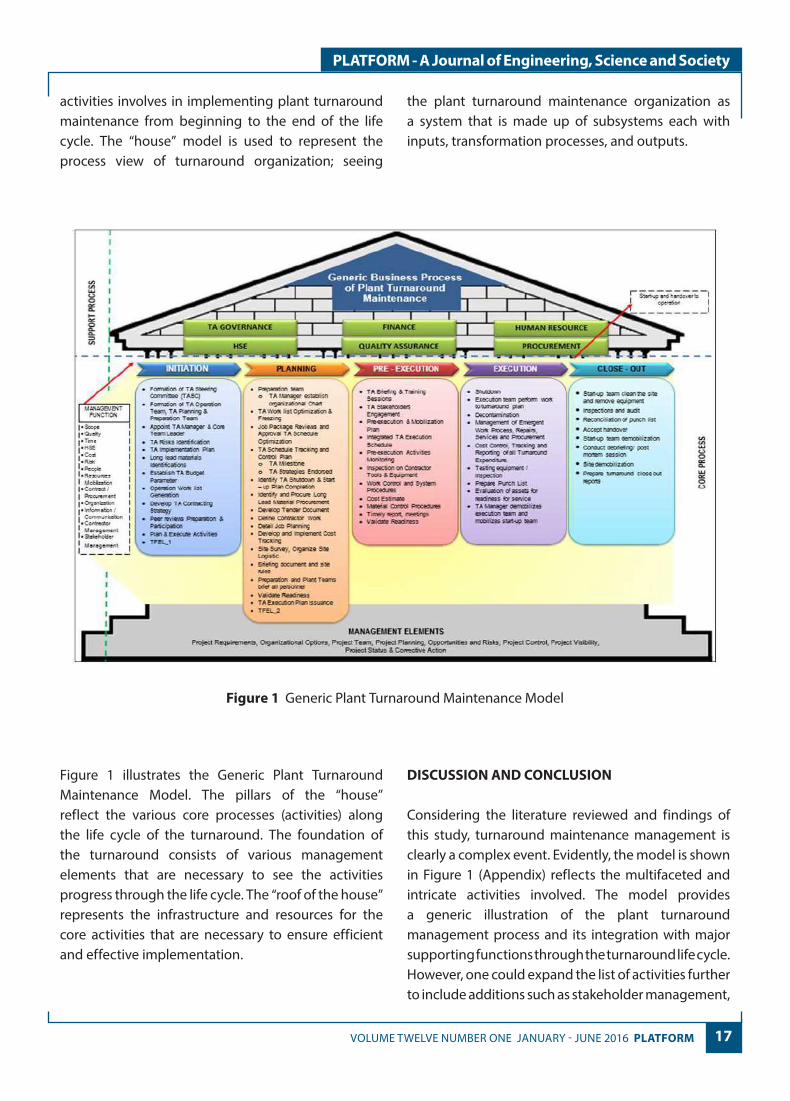
activities involves in implementing plant turnaround maintenance from beginning to the end of the life cycle. The “house” model is used to represent the process view of turnaround organization; seeing
the plant turnaround maintenance organization as a system that is made up of subsystems each with inputs, transformation processes, and outputs.
Figure 1 Generic Plant Turnaround Maintenance Model
Figure 1 illustrates the Generic Plant Turnaround Maintenance Model. The pillars of the “house” reflect the various core processes (activities) along the life cycle of the turnaround. The foundation of the turnaround consists of various management elements that are necessary to see the activities progress through the life cycle. The “roof of the house” represents the infrastructure and resources for the core activities that are necessary to ensure efficient and effective implementation.
DISCUSSION AND CONCLUSION
Considering the literature reviewed and findings of this study, turnaround maintenance management is clearly a complex event. Evidently, the model is shown in Figure 1 (Appendix) reflects the multifaceted and intricate activities involved. The model provides a generic illustration of the plant turnaround management process and its integration with major supporting functions through the turnaround life cycle. However, one could expand the list of activities further to include additions such as stakeholder management,
18 PLATFORM VOLUME TWELVE NUMBER ONE JANUARY - JUNE 2016
PLATFORM - A Journal of Engineering, Science and Society
cash flow management, data management, document storage and retrieval management, the management of cultural differences, conflict management, public relations management, critical supply chain buffer management, customer relations management, and even knowledge management. How best to depict the turnaround management graphically depends partly on the purpose of the model illustration.
This model represents an initial step towards a progression to a broader strategic view of managing plant turnaround maintenance. Further enhancement to the turnaround management model is possible by examining past works thoroughly as lessons learned and build on the past successes.
ACKNOWLEDGEMENTS
This research is funded by Ministry of Science, Technology and Innovation (MOSTI) Malaysia through e-Science Fund and Universiti Teknologi PETRONAS Malaysia through Graduate Assistantship Scheme. Authors are highly thankful to both institutions for their support.
REFERENCES
[1] G. DeBakey, “A Culture of Turnaround Excellence: How a mid-size re�ning company went after it”, 2007. [Online] Retrieved March 30, 2009 from http://www.ap-networks.com.
[2] J. Gandolfo and B. Vichich, “Turnaround Performance Excellence: Breaking the barriers of Traditional Learning”, 2007. [Online] Retrieved March 30, 2009 from http://www.ap-networks.com.
[3] J. Roup, “Strategy Maximizes Turnaround Performance”, in Oil & Gas Journal, Vol 102, No 20, pp 46_53, 2004.
[4] G. DeBakey, B. Samman, S.M. Sulaiman, K. Blanchar and D. Edmundson, “Maximising Plant Productivity”, 2007. [Online] Retrieved March 30, 2009 from http://www.ap-networks.com.
[5] B. Vichich, "Study measures E�ect of Leading Indicators of Plant Turnaround", in Oil & Gas Journal, 105(19), pp 48-54, 2007
[6] R. Oliver, “Complete Planning for Maintenance Turnarounds will Ensure Success”, in Oil & Gas Journal, Vol 100, No 17, pp 54_62, 2002.
[7] M. Raou� and A.R. Fayek, “Process Improvement for Power Plant Turnaround Planning and Management”, in International Journal of Architecture, Engineering and Construction, Volume 3, No 3, pp 168_181, 2014.
[8] Z. Ghazali and M. Halib, “The Forgotten Dimension: Work Culture in Plant Turnaround Maintenance of a Malaysian Petrochemical Company”, in Global Business and Management Research: An International Journal, Vol. 6, No. 3, pp 197–204, 2014.
[9] Z. Ghazali and M. Halib, “Managing plant turnaround maintenance in Malaysian process-based industries: A study on centralisation, formalisation and plant technology”, in Int. J. Applied Management Science, Vol. 7, No. 1, pp 59_80, 2015.
[10] A. Kelly, Maintenance organization and system. Oxford, England: Butterworth-Heinemann, 1997.
[11] T. Lenahan, Turnaround Management. Oxford, England: Butterworth-Heinemann, 1999.
[12] J. Levitt, Managing Maintenance Shutdowns and Outages. New York: Industrial Press, 2004.
[13] Z. Ghazali, M. Halib, “The Organization of Plant Turnaround Maintenance in Process-Based Industries: Analytical Framework and Generic Processes”, Journal of International Business Management & Research, Vol 2, Issue 3, 2011.
[14] S.C. Certo and S.T. Certo, Modern Management, 10th Edition, Upper Saddle River: Pearson Education Inc., 2006.
[15] F. Trompenaars and P. H. Coebergh, Management Models, Kuala Lumpur: MPH Group Publishing, 2015.

19VOLUME TWELVE NUMBER ONE JANUARY - JUNE 2016 PLATFORM
PLATFORM - A Journal of Engineering, Science and Society
AUTHORS' INFORMATION
Dr Zulkipli Ghazali received his Bachelor in Mechanical Engineering from the Universiti Teknologi Malaysia (1983), MBA from the International Management Centre, UK (1998) and PhD from the Universiti Teknologi MARA Malaysia (2010).
He is currently an Associate Professor at the Department of Management and Humanities, Universiti Teknologi PETRONAS, Malaysia. He has 20 years industrial experience prior to his current academic appointment. He is a graduate member of the Institute of Engineers Malaysia (IEM) and a member of the Society of Petroleum Engineers (SPE).
His research and academic interests include management and organizational studies with special focus on Organization and Management of Plant Turnaround Maintenance in petrochemical industries. Other major research and consultancy works that have been completed include “A Behavioral Study on Baronia Offshore Platform Personnel of PETRONAS Carigali Sdn Bhd, an international research project on “The Effectiveness Study on Greater Nile Petroleum Operating Company’s Community Development Projects in the Republic of Sudan” in collaboration with the University of Khartoum, Sudan and University of Juba, Republic of South Sudan, and a consultancy research on “The Behavioral and Mindset Change for PETRONAS Lube Blending Plant”. His current research among others include (1) Stakeholders Issues and Analysis on the Social, Economic and Environmental Implications of CO2 – Natural Gas Value Chain Program, (2) Development of Management and Organization Model for Plant Turnaround Maintenance in Malaysian Process-based Industries (3) The development of Customer Value Co-Creation Behavior Model in Malaysian Retail Industry.
He received a number of national research grants namely from PETRONAS Gas Berhad, ERGS, Sciencefund, MyRA, and FRGS. He also received an international grant from the Greater Nile Petroleum Operating Company, Sudan.

20 PLATFORM VOLUME TWELVE NUMBER ONE JANUARY - JUNE 2016
PLATFORM - A Journal of Engineering, Science and Society
ELASTIC PROPERTIES AND SEISMIC ATTRIBUTES STUDYOF SOFT SHALE AND GAS SAND IN SABAH BASIN
Adelynna Shirley anak Penguang1, Luluan Almanna Lubis1,2, Deva Prasad Ghosh2
1Petroleum Geoscience Department,2Centre of Excellence in Subsurface Seismic Imaging & Hydrocarbon Prediction,
Universiti Teknologi PETRONAS,
Email: [email protected] 1,[email protected]
ABSTRACT
The acoustic impedance of shale are mostly higher or di�erent than the acoustic impedance of reservoir sand and is consistent with the gamma ray response which is the usual case that helps us to delineate the sand from shale. However, in Sabah basin, the shale has almost similar acoustic impedance (AI) response with the gas sand and is inconsistent with the gamma ray response which complicates the �uid and lithology discrimination. Therefore, in this paper, rock physics models, elastic moduli and seismic attributes are generated and analyzed to further understand the properties of the soft shale cap rock and gas sand. Based on the results, elastic moduli such as the velocity ratio, Poisson’s ratio, Lambda-Mu-Rho (LMR) and scaled inverse quality (Q) ratio are better than the acoustic impedance in delineating the soft shale and gas sand and is consistent with the gamma ray response. The RMS amplitude attribute discriminates the gas sand from the soft shale while the Relative Acoustic Impedance attribute increases the impedance contrast between the intervals, compared to the seismic section alone, which can be used to re�ne the horizon interpretation. The results reveal more e�ective elastic moduli which can be used for further study such as the inversion process and also reduce pitfall during well log and seismic interpretation.
Keywords : soft shale; gas sand; elastic moduli, rock physics model, seismic attributes
INTRODUCTION
Elastic properties of reservoirs are widely exploited over the past few years in the oil and gas exploration industry. The elastic properties such as the impedance, velocity and density are related to the reservoir properties which are the porosity, volume of shale and water saturation [1]. Thus, interpreter depends on the elastic properties as an indicator of fluids and lithology type to refine the well log analysis and improve the seismic interpretation by inverting the seismic data to elastic properties through a process known as seismic inversion. Hydrocarbon sand usually has different elastic properties which distinguish them from the shale and non-reservoir rocks.
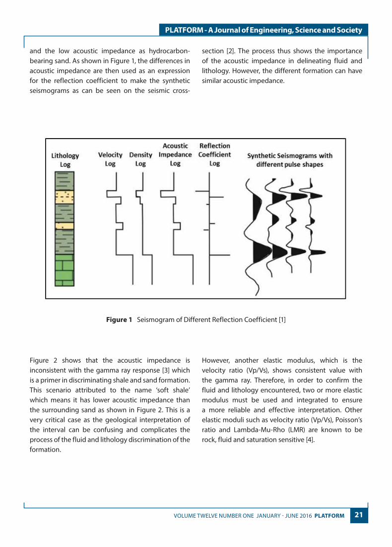
For example, acoustic impedance (AI), which is the product of velocity and density [2], is affected by different lithology type as shown in Figure 1.
When a velocity wave encounter a hard subsurface formation with higher density and compacted (less presence of fluid and porosity), a high acoustic impedance value would be produced, which usually indicates shale. A softer formation will produce a lower acoustic impedance value than the hard formation. For example, a gas sand interval with low density and gas content that slows the velocity of the sound will produce a lower acoustic impedance value [2]. Therefore in the most clastic reservoir, we usually indicate the high acoustic impedance as shale
21VOLUME TWELVE NUMBER ONE JANUARY - JUNE 2016 PLATFORM
PLATFORM - A Journal of Engineering, Science and Society
and the low acoustic impedance as hydrocarbon-bearing sand. As shown in Figure 1, the differences in acoustic impedance are then used as an expression for the reflection coefficient to make the synthetic seismograms as can be seen on the seismic cross-
section [2]. The process thus shows the importance of the acoustic impedance in delineating fluid and lithology. However, the different formation can have similar acoustic impedance.
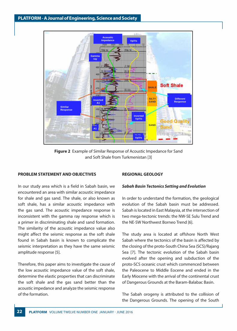
Figure 2 shows that the acoustic impedance is inconsistent with the gamma ray response [3] which is a primer in discriminating shale and sand formation. This scenario attributed to the name ‘soft shale’ which means it has lower acoustic impedance than the surrounding sand as shown in Figure 2. This is a very critical case as the geological interpretation of the interval can be confusing and complicates the process of the fluid and lithology discrimination of the formation.
However, another elastic modulus, which is the velocity ratio (Vp/Vs), shows consistent value with the gamma ray. Therefore, in order to confirm the fluid and lithology encountered, two or more elastic modulus must be used and integrated to ensure a more reliable and effective interpretation. Other elastic moduli such as velocity ratio (Vp/Vs), Poisson’s ratio and Lambda-Mu-Rho (LMR) are known to be rock, fluid and saturation sensitive [4].
Figure 1 Seismogram of Different Reflection Coefficient [1]
22 PLATFORM VOLUME TWELVE NUMBER ONE JANUARY - JUNE 2016
PLATFORM - A Journal of Engineering, Science and Society
Figure 2 Example of Similar Response of Acoustic Impedance for Sandand Soft Shale from Turkmenistan [3]
PROBLEM STATEMENT AND OBJECTIVES
In our study area which is a field in Sabah basin, we encountered an area with similar acoustic impedance for shale and gas sand. The shale, or also known as soft shale, has a similar acoustic impedance with the gas sand. The acoustic impedance response is inconsistent with the gamma ray response which is a primer in discriminating shale and sand formation. The similarity of the acoustic impedance value also might affect the seismic response as the soft shale found in Sabah basin is known to complicate the seismic interpretation as they have the same seismic amplitude response [5].
Therefore, this paper aims to investigate the cause of the low acoustic impedance value of the soft shale, determine the elastic properties that can discriminate the soft shale and the gas sand better than the acoustic impedance and analyze the seismic response of the formation.
REGIONAL GEOLOGY
Sabah Basin Tectonics Setting and Evolution
In order to understand the formation, the geological evolution of the Sabah basin must be addressed. Sabah is located in East Malaysia, at the intersection of two mega-tectonic trends: the NW-SE Sulu Trend and the NE-SW Northwest Borneo Trend [6].
The study area is located at offshore North West Sabah where the tectonics of the basin is affected by the closing of the proto-South China Sea (SCS)/Rajang Sea [7]. The tectonic evolution of the Sabah basin evolved after the opening and subduction of the proto-SCS oceanic crust which commenced between the Paleocene to Middle Eocene and ended in the Early Miocene with the arrival of the continental crust of Dangerous Grounds at the Baram-Balabac Basin.
The Sabah orogeny is attributed to the collision of the Dangerous Grounds. The opening of the South
SHALE
SILTYSAND
SAND
SimilarResponse
AcousticImpedance Vp/Vs
Gammaray
InvertedA1
InvertedVp/Vs
Vp/Vs
DifferentResponse
A1

23VOLUME TWELVE NUMBER ONE JANUARY - JUNE 2016 PLATFORM
PLATFORM - A Journal of Engineering, Science and Society
China Sea resulted in the drifting and collision of Dangerous Grounds and Reed Bank with Sabah margin [7]. According to Tan & Lamy [6], the collision and subduction of South China Sea oceanic crust beneath Borneo deposited and formed deep marine sediments into accretionary prisms since late Eocene. In early Middle Miocene, the collision and subduction has uplifted and eroded the accretionary prism and formed the Deep Regional Unconformity and caused NW progradation in the Inboard Belt. The subduction reduced in middle Late Miocene and was followed by tectonic activities such as compressional deformation, folding, uplifting, and erosion which formed the Shallow Regional Unconformity, N-S shear zone, Outboard Belt and East Baram Delta. The Outboard Belt and Baram Delta has thick prograding sedimentary wedge to the northwest from Late
Miocene and Holocene, and experience deformation in the late Pliocene which produced anticlines and faults. The Inboard Belt meanwhile continued to be stable and shallow but eroded continuously until Stage IVF times until Holocene.
The study area’s depositional system consists of mostly deltaic sediments and was moving further offshore northwest in each deltaic system [7]. Tan & Lamy [6] stated that the hydrocarbons are found in the Stages IVC, IVD and IVE shallow marine sands.The hydrocarbon in this field is mostly found in the Stage IVC sediments near the Morris fault at offshore Northwest Sabah, Malaysia [8]. The gas sand with the similar acoustic impedance as shale is from Stage IVC shallow marine sand and prograding deltaic sands [7].
Study Area
Figure 3 Map of Study Area (Modified from Google Map, 2016)
SABAH
SARAWAK
PENINSULARMALAYSIA
FIELD UTP S
24 PLATFORM VOLUME TWELVE NUMBER ONE JANUARY - JUNE 2016
PLATFORM - A Journal of Engineering, Science and Society
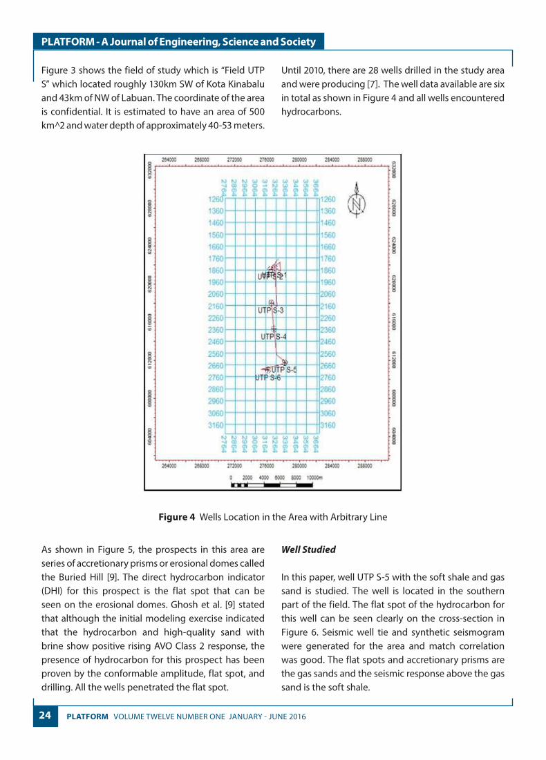
Figure 3 shows the field of study which is “Field UTP S” which located roughly 130km SW of Kota Kinabalu and 43km of NW of Labuan. The coordinate of the area is confidential. It is estimated to have an area of 500 km^2 and water depth of approximately 40-53 meters.
Until 2010, there are 28 wells drilled in the study area and were producing [7]. The well data available are six in total as shown in Figure 4 and all wells encountered hydrocarbons.
As shown in Figure 5, the prospects in this area are series of accretionary prisms or erosional domes called the Buried Hill [9]. The direct hydrocarbon indicator (DHI) for this prospect is the flat spot that can be seen on the erosional domes. Ghosh et al. [9] stated that although the initial modeling exercise indicated that the hydrocarbon and high-quality sand with brine show positive rising AVO Class 2 response, the presence of hydrocarbon for this prospect has been proven by the conformable amplitude, flat spot, and drilling. All the wells penetrated the flat spot.
Well Studied
In this paper, well UTP S-5 with the soft shale and gas sand is studied. The well is located in the southern part of the field. The flat spot of the hydrocarbon for this well can be seen clearly on the cross-section in Figure 6. Seismic well tie and synthetic seismogram were generated for the area and match correlation was good. The flat spots and accretionary prisms are the gas sands and the seismic response above the gas sand is the soft shale.
Figure 4 Wells Location in the Area with Arbitrary Line

25VOLUME TWELVE NUMBER ONE JANUARY - JUNE 2016 PLATFORM
PLATFORM - A Journal of Engineering, Science and Society
Figure 5 Seismic cross-section along the well trajectory in Field UTP S
Figure 6 Cross-section of the Well and Synthetic Seismogram of Well UTP

26 PLATFORM VOLUME TWELVE NUMBER ONE JANUARY - JUNE 2016
PLATFORM - A Journal of Engineering, Science and Society
METHODOLOGY
Figure 7 shows the whole workflow of this study. The methodology used to evaluate Well UTP S-5 in this
paper is comprised of four main parts which are seismic attributes interpretation, well logs interpretation, rock physics model, and rock physics template.
Figure 7 Workflow of Study
Seismic Volume Attributes Interpretation
Seismic elastic inversion process usually carried out to get the 3-D acoustic impedance product in order to evaluate the acoustic impedance of a 3-D seismic data. However, due to time constraint, the relative acoustic impedance is generated from PETREL seismic attribute for this study. According to Subrahmanyam and Rao [10], the Relative Acoustic Impedance is a physical attribute type which is directly related to the parameters such as lithology and wave propagation and is an indicator of impedance changes, and thus an effective attribute to use for the formation. Other than the relative acoustic impedance attribute, Variance and Relative Mean Square (RMS) amplitude were also computed. According to Petrel software, Variance attribute extracts the edge volume and highlights faults or delineation while RMS amplitude shows the hydrocarbon anomaly as it computes RMS on instantaneous trace samples over a specified window. This anomaly is expected when evaluating the results of the attribute since the well-encountered
hydrocarbon. Seismic are used in this study instead of using only wells in order to extrapolate the data outside the well [11]. The geometry and extension of the formation from the well log will be shown in seismic section.
Well Logs
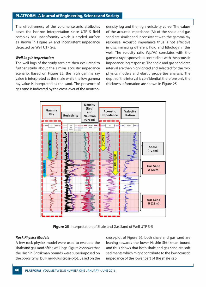
The well log data of Well UTP S-5 were interpreted and petrophysical analysis (e.g. porosity, volume of shale and water saturation) is carried out. The interval of interest which are the soft shale and gas zone were identified as supported by the well log response and final well report by PETRONAS.
After the petrophysical analysis, elastic moduli other than acoustic impedance are generated to evaluate the sensitivity towards the soft shale and the gas sand. The elastic moduli generated are velocity ratio (Vp/Vs), Poisson’s ratio, Lambda-Rho, Mu-Rho, scaled inverse Qp (SQp) and scaled inverse Qs (SQs). The derivations of the elastic moduli are shown in Table 1.

27VOLUME TWELVE NUMBER ONE JANUARY - JUNE 2016 PLATFORM
PLATFORM - A Journal of Engineering, Science and Society
Table 1 Elastic Properties
Elastic Properties Derivation
Velocity Ratio (Vp/Vs) Compressional Sonic Log/ Shear Sonic Log
Poisson’s ratio
LambdaRho Lame Parameter* Density
MuRho Shear Modulus*Density
Scaled Inverse Qp
Scaled Inverse Qs SQP = 10 1 (M / G)
3 p (3M / G - 2)
Rock Physics ModelThe petrophysical analysis result and elastic moduli were then analyzed using a few appropriate rock physics models. The rock physics model provides the bounds which represent the possible maximum and minimum volume fractions of composite rock content and thus can be used to quality control (QC) our petrophysical analysis and to evaluate the elastic modulus computed. The rock physics models used in this study are Hashin-Shtrikman bounds, Friable Sand and Friable Shale and Constant Cement model.
The friable-sand model [12], also known as the unconsolidated model, is a model that describes the velocity-porosity behavior versus sorting at a specific effective pressure which was introduced by Dvorkin and Nur (1996). The model has the “well sorted” end member where it is assumed to have a critical porosity of 0.4.. The “well sorted” end member is modeled using the Hertz-Mindlin theory (Mindlin, 1949) where the bulk modulus is defined using equation 1 and the shear modulus is defined as Equation 2 as shown below;
KHM = Bullk ModulusμHM= Shear Modulusn = coordination number Øc=critical prosityμ = shear modulusv = Poisson’s ratioP = effective pressure
The value of the Hertz-Mindlin bound is then used in Equation 3 to determine the bulk modulus and in Equation 4 to determine the shear modulus for varying porosity value of the friable sand mixture as shown below;
WhereKdry = Dry bulk modulusμdry = Shear modulusKHM = Bulk modulus at critical porosityμHM = Shear modulus at critical porosityØ = porosityØc =critical porosity
28 PLATFORM VOLUME TWELVE NUMBER ONE JANUARY - JUNE 2016
PLATFORM - A Journal of Engineering, Science and Society
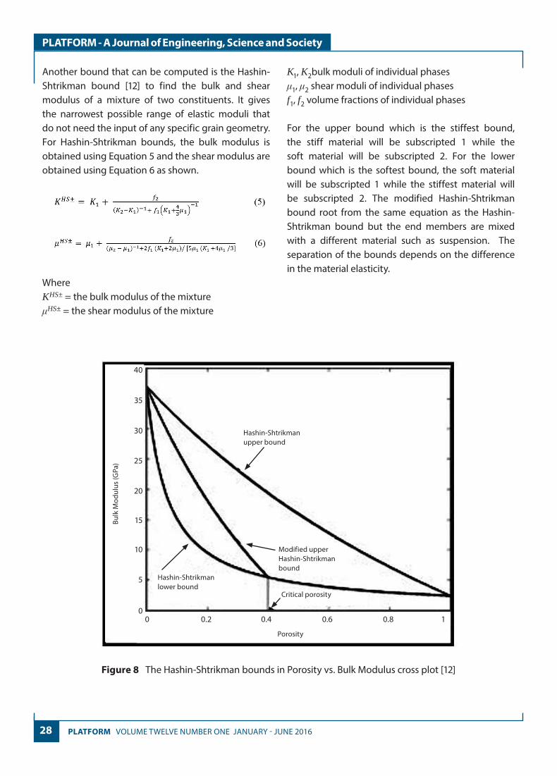
Another bound that can be computed is the Hashin-Shtrikman bound [12] to find the bulk and shear modulus of a mixture of two constituents. It gives the narrowest possible range of elastic moduli that do not need the input of any specific grain geometry. For Hashin-Shtrikman bounds, the bulk modulus is obtained using Equation 5 and the shear modulus are obtained using Equation 6 as shown.
WhereKHS± = the bulk modulus of the mixtureμHS± = the shear modulus of the mixture
K1, K2bulk moduli of individual phasesμ1, μ2 shear moduli of individual phasesf1, f2 volume fractions of individual phases
For the upper bound which is the stiffest bound, the stiff material will be subscripted 1 while the soft material will be subscripted 2. For the lower bound which is the softest bound, the soft material will be subscripted 1 while the stiffest material will be subscripted 2. The modified Hashin-Shtrikman bound root from the same equation as the Hashin-Shtrikman bound but the end members are mixed with a different material such as suspension. The separation of the bounds depends on the difference in the material elasticity.
Hashin-Shtrikmanupper bound
Modified upperHashin-Shtrikmanbound
Hashin-Shtrikmanlower bound
Bulk
Mod
ulus
(GPa
)
Porosity
Critical porosity
0 0.2 0.4 0.6 0.8 10
5
10
15
20
25
30
35
40
Figure 8 The Hashin-Shtrikman bounds in Porosity vs. Bulk Modulus cross plot [12]
29VOLUME TWELVE NUMBER ONE JANUARY - JUNE 2016 PLATFORM
PLATFORM - A Journal of Engineering, Science and Society
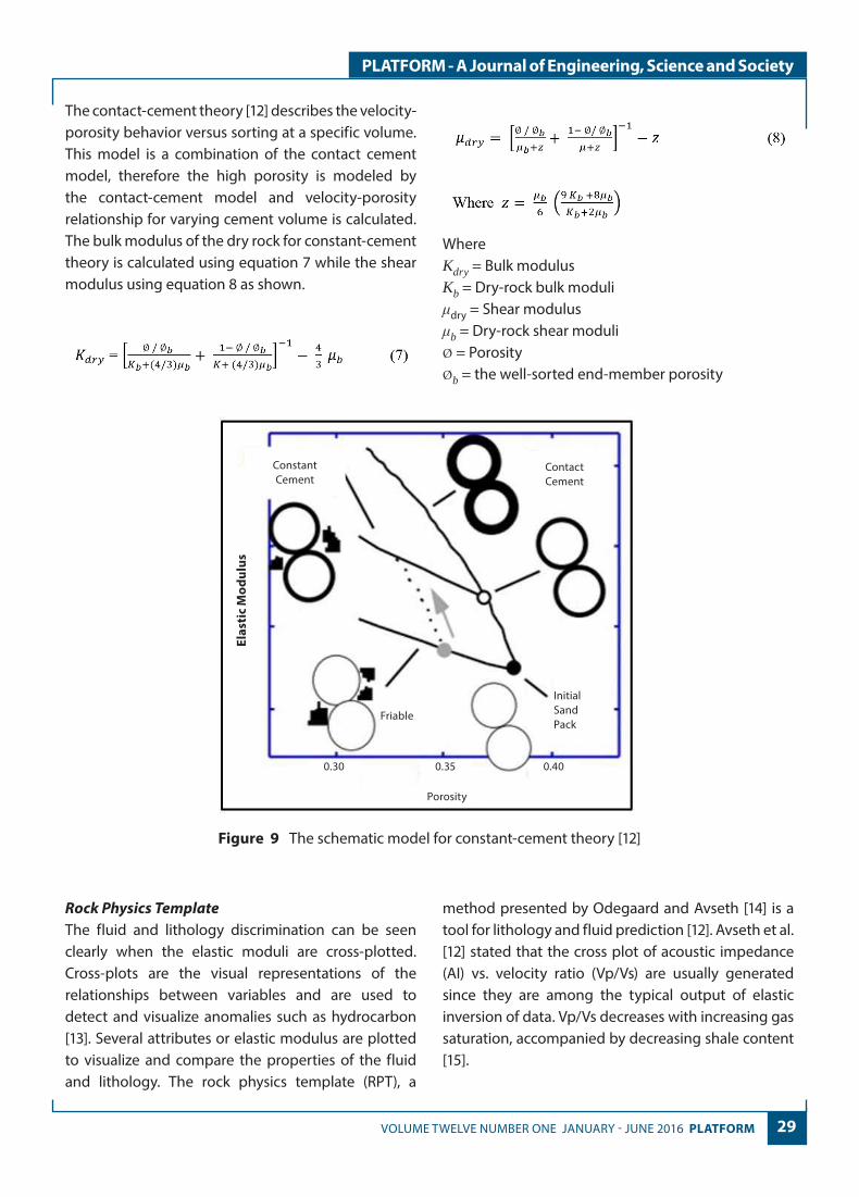
The contact-cement theory [12] describes the velocity-porosity behavior versus sorting at a specific volume. This model is a combination of the contact cement model, therefore the high porosity is modeled by the contact-cement model and velocity-porosity relationship for varying cement volume is calculated. The bulk modulus of the dry rock for constant-cement theory is calculated using equation 7 while the shear modulus using equation 8 as shown.
WhereKdry = Bulk modulusKb = Dry-rock bulk moduli μdry = Shear modulus μb = Dry-rock shear moduliØ = PorosityØb = the well-sorted end-member porosity
ContactCement
Friable
Porosity
0.30 0.35 0.40
InitialSandPack
ConstantCement
Elas
tic
Mod
ulus
Figure 9 The schematic model for constant-cement theory [12]
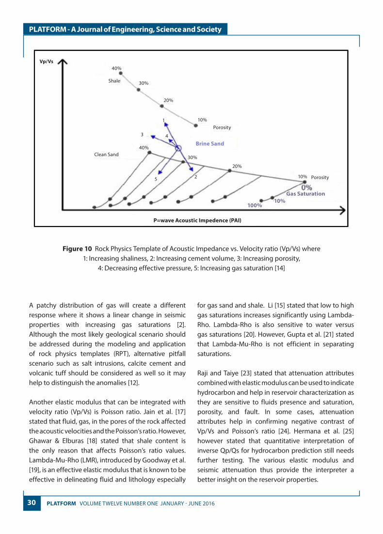
Rock Physics TemplateThe fluid and lithology discrimination can be seen clearly when the elastic moduli are cross-plotted. Cross-plots are the visual representations of the relationships between variables and are used to detect and visualize anomalies such as hydrocarbon [13]. Several attributes or elastic modulus are plotted to visualize and compare the properties of the fluid and lithology. The rock physics template (RPT), a
method presented by Odegaard and Avseth [14] is a tool for lithology and fluid prediction [12]. Avseth et al. [12] stated that the cross plot of acoustic impedance (AI) vs. velocity ratio (Vp/Vs) are usually generated since they are among the typical output of elastic inversion of data. Vp/Vs decreases with increasing gas saturation, accompanied by decreasing shale content [15].
30 PLATFORM VOLUME TWELVE NUMBER ONE JANUARY - JUNE 2016
PLATFORM - A Journal of Engineering, Science and Society
Porosity
Porosity
Vp/Vs
P=wave Acoustic Impedence (PAI)
Clean Sand
Brine Sand
Gas Saturation10%
100%
Shale
10%
10%
20%
30%
40%
20%
1
4
25
3
30%
40%
Figure 10 Rock Physics Template of Acoustic Impedance vs. Velocity ratio (Vp/Vs) where 1: Increasing shaliness, 2: Increasing cement volume, 3: Increasing porosity,
4: Decreasing effective pressure, 5: Increasing gas saturation [14]
A patchy distribution of gas will create a different response where it shows a linear change in seismic properties with increasing gas saturations [2]. Although the most likely geological scenario should be addressed during the modeling and application of rock physics templates (RPT), alternative pitfall scenario such as salt intrusions, calcite cement and volcanic tuff should be considered as well so it may help to distinguish the anomalies [12].
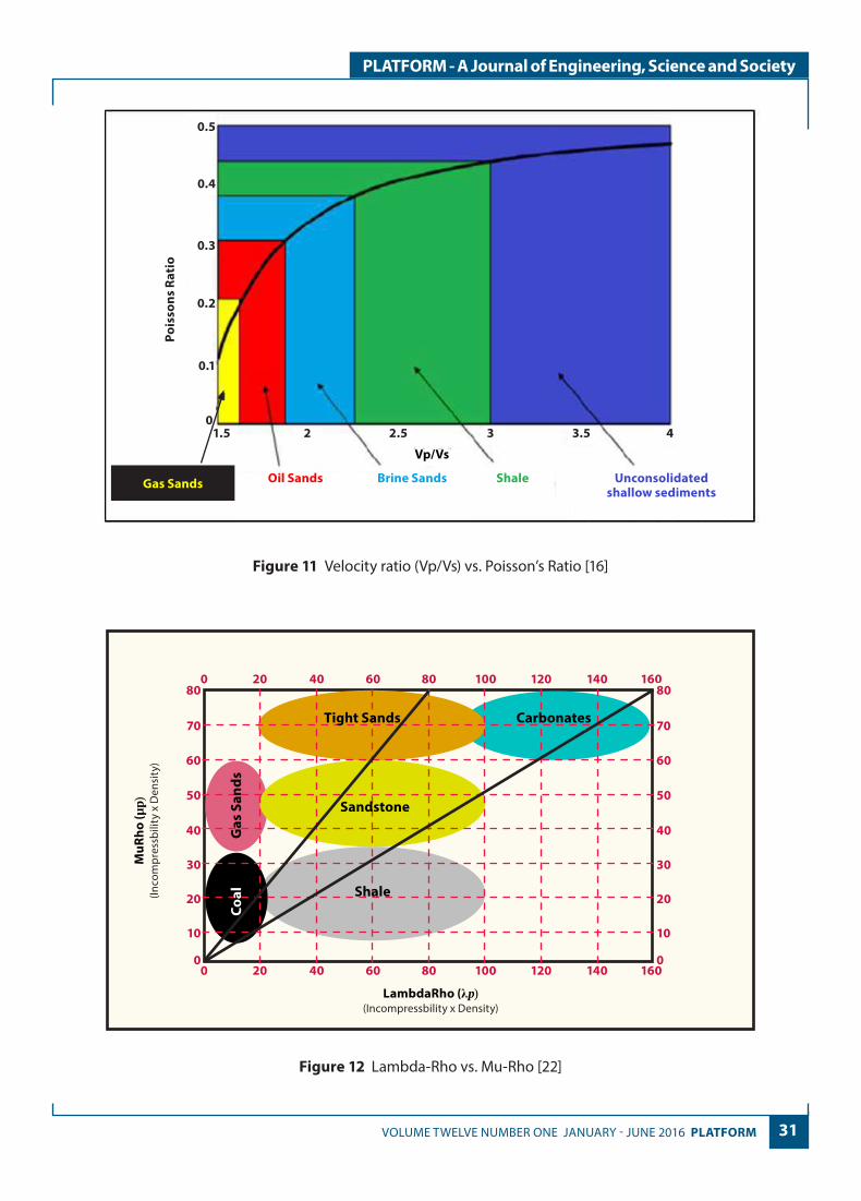
Another elastic modulus that can be integrated with velocity ratio (Vp/Vs) is Poisson ratio. Jain et al. [17] stated that fluid, gas, in the pores of the rock affected the acoustic velocities and the Poisson’s ratio. However, Ghawar & Elburas [18] stated that shale content is the only reason that affects Poisson’s ratio values. Lambda-Mu-Rho (LMR), introduced by Goodway et al. [19], is an effective elastic modulus that is known to be effective in delineating fluid and lithology especially
for gas sand and shale. Li [15] stated that low to high gas saturations increases significantly using Lambda-Rho. Lambda-Rho is also sensitive to water versus gas saturations [20]. However, Gupta et al. [21] stated that Lambda-Mu-Rho is not efficient in separating saturations.
Raji and Taiye [23] stated that attenuation attributes combined with elastic modulus can be used to indicate hydrocarbon and help in reservoir characterization as they are sensitive to fluids presence and saturation, porosity, and fault. In some cases, attenuation attributes help in confirming negative contrast of Vp/Vs and Poisson’s ratio [24]. Hermana et al. [25] however stated that quantitative interpretation of inverse Qp/Qs for hydrocarbon prediction still needs further testing. The various elastic modulus and seismic attenuation thus provide the interpreter a better insight on the reservoir properties.
31VOLUME TWELVE NUMBER ONE JANUARY - JUNE 2016 PLATFORM
PLATFORM - A Journal of Engineering, Science and Society
Pois
sons
Rat
io
1.5 2 2.5 3 3.5 4
Unconsolidatedshallow sediments
ShaleBrine Sands
Vp/Vs
Oil SandsGas Sands
0
0.1
0.2
0.3
0.4
0.5
Figure 11 Velocity ratio (Vp/Vs) vs. Poisson’s Ratio [16]
0 20 40 60 80 100 120 140 160
0 20 40 60 80 100 120 140 160
0
10
20
30
40
50
60
70
80
0
10
20
30
40
50
60
70
80
LambdaRho (λp)(Incompressbility x Density)
Shale
Coal
Gas
San
ds
Sandstone
Tight Sands Carbonates
MuR
ho (µ
p)(In
com
pres
sbili
ty x
Den
sity
)
Figure 12 Lambda-Rho vs. Mu-Rho [22]

32 PLATFORM VOLUME TWELVE NUMBER ONE JANUARY - JUNE 2016
PLATFORM - A Journal of Engineering, Science and Society
Figure 13 Scaled Inverse Qs vs. Scale Inverse Qp Template [26]
Figure 14 Cross-section of realized seismic amplitude and Variance attribute
Realized SeismicAmplitude
VarianceAttribute
33VOLUME TWELVE NUMBER ONE JANUARY - JUNE 2016 PLATFORM
PLATFORM - A Journal of Engineering, Science and Society
RESULTS AND DISCUSSION
The results and discussion are divided into a few parts which are the seismic attributes, well log evaluation, rock physics model and rock physics template.
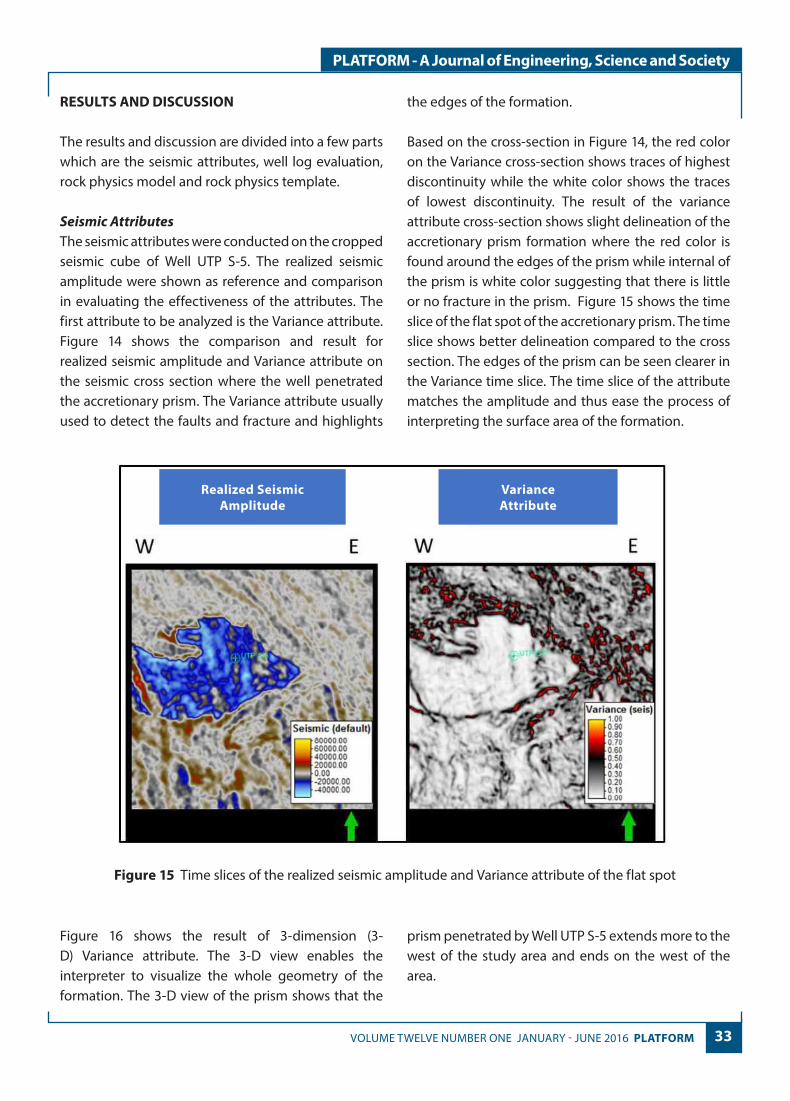
Seismic AttributesThe seismic attributes were conducted on the cropped seismic cube of Well UTP S-5. The realized seismic amplitude were shown as reference and comparison in evaluating the effectiveness of the attributes. The first attribute to be analyzed is the Variance attribute. Figure 14 shows the comparison and result for realized seismic amplitude and Variance attribute on the seismic cross section where the well penetrated the accretionary prism. The Variance attribute usually used to detect the faults and fracture and highlights
the edges of the formation.
Based on the cross-section in Figure 14, the red color on the Variance cross-section shows traces of highest discontinuity while the white color shows the traces of lowest discontinuity. The result of the variance attribute cross-section shows slight delineation of the accretionary prism formation where the red color is found around the edges of the prism while internal of the prism is white color suggesting that there is little or no fracture in the prism. Figure 15 shows the time slice of the flat spot of the accretionary prism. The time slice shows better delineation compared to the cross section. The edges of the prism can be seen clearer in the Variance time slice. The time slice of the attribute matches the amplitude and thus ease the process of interpreting the surface area of the formation.
Realized SeismicAmplitude
VarianceAttribute
Figure 15 Time slices of the realized seismic amplitude and Variance attribute of the flat spot
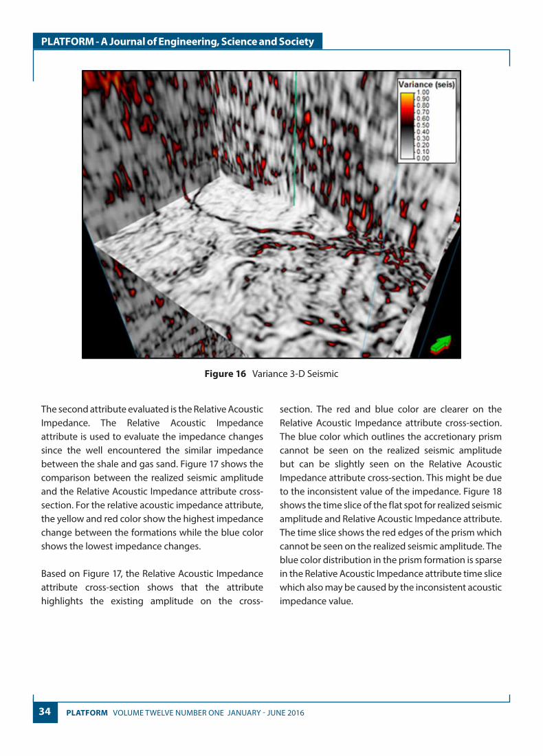
Figure 16 shows the result of 3-dimension (3-D) Variance attribute. The 3-D view enables the interpreter to visualize the whole geometry of the formation. The 3-D view of the prism shows that the
prism penetrated by Well UTP S-5 extends more to the west of the study area and ends on the west of the area.
34 PLATFORM VOLUME TWELVE NUMBER ONE JANUARY - JUNE 2016
PLATFORM - A Journal of Engineering, Science and Society
Figure 16 Variance 3-D Seismic
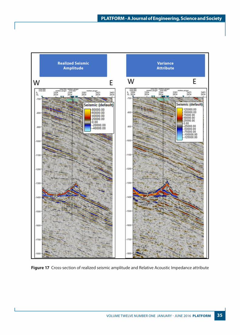
The second attribute evaluated is the Relative Acoustic Impedance. The Relative Acoustic Impedance attribute is used to evaluate the impedance changes since the well encountered the similar impedance between the shale and gas sand. Figure 17 shows the comparison between the realized seismic amplitude and the Relative Acoustic Impedance attribute cross-section. For the relative acoustic impedance attribute, the yellow and red color show the highest impedance change between the formations while the blue color shows the lowest impedance changes.
Based on Figure 17, the Relative Acoustic Impedance attribute cross-section shows that the attribute highlights the existing amplitude on the cross-
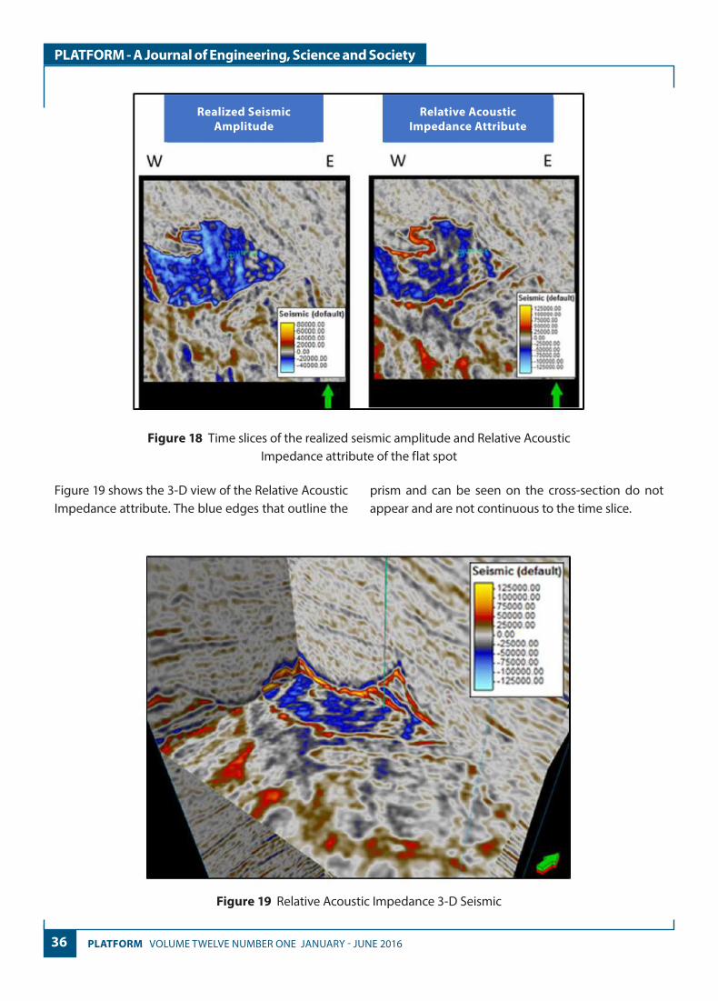
section. The red and blue color are clearer on the Relative Acoustic Impedance attribute cross-section. The blue color which outlines the accretionary prism cannot be seen on the realized seismic amplitude but can be slightly seen on the Relative Acoustic Impedance attribute cross-section. This might be due to the inconsistent value of the impedance. Figure 18 shows the time slice of the flat spot for realized seismic amplitude and Relative Acoustic Impedance attribute. The time slice shows the red edges of the prism which cannot be seen on the realized seismic amplitude. The blue color distribution in the prism formation is sparse in the Relative Acoustic Impedance attribute time slice which also may be caused by the inconsistent acoustic impedance value.
35VOLUME TWELVE NUMBER ONE JANUARY - JUNE 2016 PLATFORM
PLATFORM - A Journal of Engineering, Science and Society
Realized SeismicAmplitude
VarianceAttribute
Figure 17 Cross-section of realized seismic amplitude and Relative Acoustic Impedance attribute
36 PLATFORM VOLUME TWELVE NUMBER ONE JANUARY - JUNE 2016
PLATFORM - A Journal of Engineering, Science and Society
Realized SeismicAmplitude
Relative AcousticImpedance Attribute
Figure 18 Time slices of the realized seismic amplitude and Relative Acoustic Impedance attribute of the flat spot
Figure 19 shows the 3-D view of the Relative Acoustic Impedance attribute. The blue edges that outline the
prism and can be seen on the cross-section do not appear and are not continuous to the time slice.
Figure 19 Relative Acoustic Impedance 3-D Seismic

37VOLUME TWELVE NUMBER ONE JANUARY - JUNE 2016 PLATFORM
PLATFORM - A Journal of Engineering, Science and Society
Figure 20 shows the cross-section of the realized seismic amplitude and the RMS amplitude attribute result. The RMS amplitude is used to highlight the anomaly which acts as direct hydrocarbon indicator.
The Well UTP S-5 penetrates hydrocarbon sand and the result is supported by the RMS amplitude. The ‘warm’ red color indicates hydrocarbon in the accretionary prism.
Realized SeismicAmplitude
RMS AmplitudeAttribute
Figure 20 Cross-sections of realized seismic amplitude and RMS amplitude
Figure 21 shows the time slice of the realized seismic amplitude and RMS amplitude of the flat spot. The RMS amplitude matches the amplitude and shows that the hydrocarbon anomaly is present inside the
prism and might extend to the west of the prism. The RMS amplitude also distinguish the hydrocarbon sands from the surrounding area.

38 PLATFORM VOLUME TWELVE NUMBER ONE JANUARY - JUNE 2016
PLATFORM - A Journal of Engineering, Science and Society
Realized SeismicAmplitude
RMS AmplitudeAttribute
Seismic (default)- 80000.00- 60000.00- 40000.00- 20000.00- 0.00- -20000.00- -40000.00
Seismic (default)
- 30000.00- 25000.00- 20000.00- 15000.00- 10000.00- 5000.00- 0.00
Figure 21 Time slices of the realized seismic amplitude and RMS Amplitude attribute of the flat spot
Figure 22 shows the 3-D view of the RMS amplitude attribute. The RMS amplitude of this cropped volume
shows the consistent anomaly along the prism and the geometry extension of the hydrocarbon sand.
Seismic (default)
- 30000.00- 25000.00- 20000.00- 15000.00- 10000.00- 5000.00- 0.00
Figure 22 RMS Amplitude 3-D Seismic

39VOLUME TWELVE NUMBER ONE JANUARY - JUNE 2016 PLATFORM
PLATFORM - A Journal of Engineering, Science and Society
Based on the results, the attributes supported the amplitude anomaly response. The attributes correlate to the anomaly of the flat spot on the seismic amplitude section penetrated by Well UTP S-5. The time slices of the attributes clearly confirm the cut-off of the hydrocarbon area when compared with the realized seismic amplitude time slice. For the
Variance attribute, the result on the cross-section is slightly dimmed compared to the Relative Acoustic Impedance and RMS Amplitude cross-section but is clearer on the time slice section. The attributes are combined and compared as shown in Figure 23 to increase confidence.
RMS AmplitudeTime Slice
Seismic (default) Seismic (default)- 30000.00- 25000.00- 20000.00- 15000.00- 10000.00- 5000.00- 0.00
- 125000.00- 100000.00- 75000.00- 50000.00- 25000.00- 0.00- -25000.00- -50000.00- -75000.00- -100000.00- -125000.00
Relative AcousticImpedance Cross-section
Figure 23 Relative Acoustic Impedance Cross-section and RMS amplitude Time Slice with Well UTP S-5
RMS AmplitudeTime Slice
Relative AcousticImpedance Cross Section
Seismic (default)- 30000.00- 25000.00- 20000.00- 15000.00- 10000.00- 5000.00- 0.00
Seismic (default)- 125000.00- 100000.00- 75000.00- 50000.00- 25000.00- 0.00- -25000.00- -50000.00- -75000.00- -100000.00- -125000.00
- .1000.00
- .1100.00
- .1200.00
- .1300.00
- .1400.00
- .1500.00
- .1600.00
Elevation time (ms)
Figure 24 Unconformity surface of the formation
40 PLATFORM VOLUME TWELVE NUMBER ONE JANUARY - JUNE 2016
PLATFORM - A Journal of Engineering, Science and Society
The effectiveness of the volume seismic attributes eases the horizon interpretation since UTP S field complex has unconformity which is eroded surface as shown in Figure 24 and inconsistent impedance detected by Well UTP S-5.
Well Log InterpretationThe well logs of the study area are then evaluated to further study about the similar acoustic impedance scenario. Based on Figure 25, the high gamma ray value is interpreted as the shale while the low gamma ray value is interpreted as the sand. The presence of gas sand is indicated by the cross-over of the neutron-
density log and the high resistivity curve. The values of the acoustic impedance (AI) of the shale and gas sand are similar and inconsistent with the gamma ray response. Acoustic impedance thus is not effective in discriminating different fluid and lithology in this well. The velocity ratio (Vp/Vs) correlates with the gamma ray response but contradicts with the acoustic impedance log response. The shale and gas sand data interval are then highlighted and selected for the rock physics models and elastic properties analysis. The depth of the interval is confidential, therefore only the thickness information are shown in Figure 25.
GammaRay Resistivity
ValocityRation
Shale(~27m)
Gas SandA (20m)
Gas SandB (23m)
Density(Red)and
Neutron(Green)
AcousticImpedance
Figure 25 Interpretation of Shale and Gas Sand of Well UTP S-5
Rock Physics ModelsA few rock physics model were used to evaluate the shale and gas sand of the well logs. Figure 26 shows that the Hashin-Shtrikman bounds were superimposed on the porosity vs. bulk modulus cross-plot. Based on the
cross-plot of Figure 26, both shale and gas sand are leaning towards the lower Hashin-Shtrikman bound and thus shows that both shale and gas sand are soft sediments which might contribute to the low acoustic impedance of the lower part of the shale cap.

41VOLUME TWELVE NUMBER ONE JANUARY - JUNE 2016 PLATFORM
PLATFORM - A Journal of Engineering, Science and Society
Upper HS
Shale Gas Sands
Lower HS
Modified HS
00
5.0
10
15
20
25
30
35
0.1 0.2 0.3 0.4 0.5 0.6 0.7 0.8 0.9 1.0
Porosity (fraction)
Bilk
Mod
ulus
(GPa
)
Figure 26 Hashin-Shtrikman Lower, Upper and Modified Bound
The friable shale, friable sand and contact cement lines were imposed on the porosity vs. P-wave velocity (Vp) cross-plot as shown in Figure 27. Based on the cross-plot of Figure 27, the shale and gas sand are both
further away from the friable shale line where the gas sand is leaning towards the friable sand line and the contact cement line which suggests that the gas sand is slightly cemented.
Constant Cement
Shale
Gas Sands
Friable Shale
Friable Sand
0
0
1000
2000
3000
4000
5000
6000
0.1 0.2 0.3 0.4 0.5 0.6 0.7 0.8 0.9 1.0
Porosity (fraction)
P-w
ave
Velo
city
, Vp
(m/s
)
Figure 27 Friable Sand, Friable Shale and Constant Cement Model

42 PLATFORM VOLUME TWELVE NUMBER ONE JANUARY - JUNE 2016
PLATFORM - A Journal of Engineering, Science and Society
The results show that the petrophysical results are in the range of the rock physics model bounds and therefore act as guidance to quality control (QC) our analysis.
Elastic Properties Crossplot AnalysisMsolo and Gidlow [27] stated that the most commonly used rock physics template (RPT) is acoustic impedance (AI) vs. velocity ratio (Vp/Vs) since it is a very useful template and separates the lithology, show porosity changes and discriminates pore fluids type. Since
the acoustic impedance couldn’t differentiate the soft shale and gas sand effectively, other cross-plots of elastic properties were also computed to illustrate the fluid and lithology discrimination. Among the cross plot computed are Vp/Vs vs. Poisson’s ratio, Lambda-Rho vs. Mu-Rho and scaled inverse Qs (SQs) vs. scaled inverse Qp (SQp). The cross-plot shows that the other elastic properties such as velocity ratio (Vp/Vs), Lambda-Mu-Rho (LMR) and scaled inverse quality (Q) ratio are better than acoustic impedance in discriminating the soft shale and gas sand.
Based on the acoustic impedance vs. velocity ratio (Vp/Vs) cross plot in Figure 28, the acoustic impedance value of the gas sand and the shale is almost similar. Therefore, as expected, there is an overlap of the acoustic impedance values between the shale and gas sand in the cross-plot. The value of the acoustic impedance for shale is ranging around 6000 (g/cm3)/ (m/s) to 7000 (g/cm3)/ (m/s) while the value for both the gas sand is around 5000 (g/cm3)/ (m/s) to
7000 (g/cm3)/ (m/s). The velocity ratio (Vp/Vs) of the gas sand is lower than shale. The Vp/Vs value of the shale is from 2 to 2.5 while the Vp/Vs value of the gas sands is from 1.5 to 2. This shows that Vp/Vs is sensitive to change of lithology and fluid type as the velocity of the shear wave increases while the velocity of the compressional wave decreases when the saturation of hydrocarbon increase [17].
Gas Sands
Shale
Velo
city
Rat
ioo,
Vp
/Vs
(uni
tles
s)
Acoustic Impedance (g/cm3_m/s)
4500
1.0
1.25
1.50
1.75
2.0
2.25
2.50
2.75
3.0
5000 5500 6000 6500 7000 7500 85008000
Figure 28 Acoustic impedance (AI) vs. velocity ratio (Vp/Vs) cross-plot
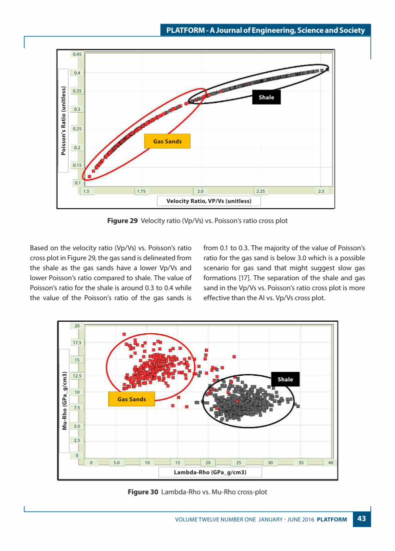
43VOLUME TWELVE NUMBER ONE JANUARY - JUNE 2016 PLATFORM
PLATFORM - A Journal of Engineering, Science and Society
Velocity Ratio, VP/Vs (unitless)
Pois
son'
s R
atio
(uni
tles
s)
Gas Sands
Shale
0.1
0.15
0.2
0.25
0.3
0.35
0.4
0.45
1.5 1.75 2.0 2.25 2.5
Figure 29 Velocity ratio (Vp/Vs) vs. Poisson’s ratio cross plot
Based on the velocity ratio (Vp/Vs) vs. Poisson’s ratio cross plot in Figure 29, the gas sand is delineated from the shale as the gas sands have a lower Vp/Vs and lower Poisson’s ratio compared to shale. The value of Poisson’s ratio for the shale is around 0.3 to 0.4 while the value of the Poisson’s ratio of the gas sands is
from 0.1 to 0.3. The majority of the value of Poisson’s ratio for the gas sand is below 3.0 which is a possible scenario for gas sand that might suggest slow gas formations [17]. The separation of the shale and gas sand in the Vp/Vs vs. Poisson’s ratio cross plot is more effective than the AI vs. Vp/Vs cross plot.
Lambda-Rho (GPa_g/cm3)
Mu-
Rho
(GPa
_g/c
m3)
Gas Sands
Shale
0
0
2.5
5.0
7.5
10
12.5
15
17.5
20
5.0 10 15 20 25 30 35 40
Figure 30 Lambda-Rho vs. Mu-Rho cross-plot
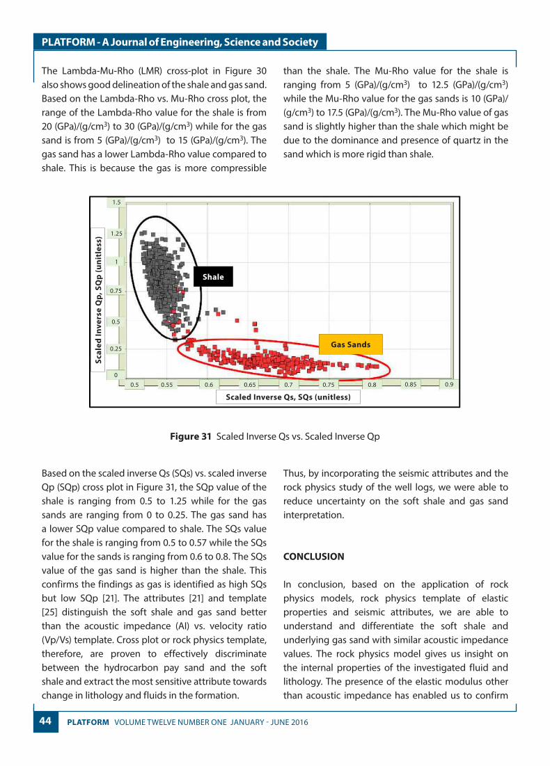
44 PLATFORM VOLUME TWELVE NUMBER ONE JANUARY - JUNE 2016
PLATFORM - A Journal of Engineering, Science and Society
The Lambda-Mu-Rho (LMR) cross-plot in Figure 30 also shows good delineation of the shale and gas sand. Based on the Lambda-Rho vs. Mu-Rho cross plot, the range of the Lambda-Rho value for the shale is from 20 (GPa)/(g/cm3) to 30 (GPa)/(g/cm3) while for the gas sand is from 5 (GPa)/(g/cm3) to 15 (GPa)/(g/cm3). The gas sand has a lower Lambda-Rho value compared to shale. This is because the gas is more compressible
than the shale. The Mu-Rho value for the shale is ranging from 5 (GPa)/(g/cm3) to 12.5 (GPa)/(g/cm3) while the Mu-Rho value for the gas sands is 10 (GPa)/(g/cm3) to 17.5 (GPa)/(g/cm3). The Mu-Rho value of gas sand is slightly higher than the shale which might be due to the dominance and presence of quartz in the sand which is more rigid than shale.
Scaled Inverse Qs, SQs (unitless)
Scal
ed In
vers
e Q
p, S
Qp
(uni
tles
s)
Gas Sands
Shale
0.50
0.25
0.5
0.75
1
1.25
1.5
0.55 0.6 0.65 0.7 0.75 0.8 0.85 0.9
Figure 31 Scaled Inverse Qs vs. Scaled Inverse Qp
Based on the scaled inverse Qs (SQs) vs. scaled inverse Qp (SQp) cross plot in Figure 31, the SQp value of the shale is ranging from 0.5 to 1.25 while for the gas sands are ranging from 0 to 0.25. The gas sand has a lower SQp value compared to shale. The SQs value for the shale is ranging from 0.5 to 0.57 while the SQs value for the sands is ranging from 0.6 to 0.8. The SQs value of the gas sand is higher than the shale. This confirms the findings as gas is identified as high SQs but low SQp [21]. The attributes [21] and template [25] distinguish the soft shale and gas sand better than the acoustic impedance (AI) vs. velocity ratio (Vp/Vs) template. Cross plot or rock physics template, therefore, are proven to effectively discriminate between the hydrocarbon pay sand and the soft shale and extract the most sensitive attribute towards change in lithology and fluids in the formation.
Thus, by incorporating the seismic attributes and the rock physics study of the well logs, we were able to reduce uncertainty on the soft shale and gas sand interpretation.
CONCLUSION
In conclusion, based on the application of rock physics models, rock physics template of elastic properties and seismic attributes, we are able to understand and differentiate the soft shale and underlying gas sand with similar acoustic impedance values. The rock physics model gives us insight on the internal properties of the investigated fluid and lithology. The presence of the elastic modulus other than acoustic impedance has enabled us to confirm
45VOLUME TWELVE NUMBER ONE JANUARY - JUNE 2016 PLATFORM
PLATFORM - A Journal of Engineering, Science and Society
our geological interpretation and the cross-plots of the elastic modulus shows good fluid and lithology discrimination which follows the universal trend of the established cross-plots. The values of the elastic modulus from our cross-plots in comparison with the values from established templates are not exactly the same but the trend of the fluid and lithology are the same and thus validated by the universal trend. This will help us in choosing the most sensitive and effective elastic properties for inversion process. Seismic attributes enable us to investigate the elastic properties in 3-dimension such as the Relative Acoustic Impedance attribute for analysis with time constraint and reveal the properties that can’t be seen on seismic amplitude section alone. The attributes are also important to reveal the geometry and extension of the investigated area. This shows that we must not depend only on one parameter but we must integrate our results and methods to increase our confidence and avoid misinterpretation.
ACKNOWLEDGEMENT
The authors wish to express their sincere gratitude and appreciation to fellow lecturers, postdoctoral researcher and peers of Petroleum Geoscience Department, Universiti Teknologi PETRONAS (UTP) and Centre of Excellence in Subsurface Seismic Imaging and Hydrocarbon Prediction for the help, encouragement, and exchange of feedback of the work. We are also grateful and would like to thank PETRONAS for the data provided to conduct this study.
REFERENCES
[1] X.G. Chi, and D.H. Han, “Lithology and �uid di�erentiation using rock physics template”, The Leading Edge, January 2009. 1424-1428, 2009.
[2] K. Bjorklykke, Petroleum Geoscience: From Sedimentary Environments to Rock Physics, Heidelberg, Germany: Springer, 2010.
[3] G. Deva and M. Brewer, Interpretation of amplitudes,2007.
[4] R. C. P. Saxena, and V. S. Bhatnagar, “Use of Various Amplitude Inversions Techniques for Seismic Reservoir Characterization”. 7th International Conference & Exposition on Petroleum Geophysics, 14-16, January, 2008.
[5] A. Tarang, and Y. Singh, “Soft Shale Complication in AVO Interpretation in Sabah Basin”. Petroleum Geology Conference & Exhibition (PGCE), 8 March, 2011.
[6] D. N. K. Tan, and J. M. Lamy, “Tectonic evolution of NW Sabah continental margin since the Late Eocene”, Geological Society Malaysia, Bulletin 27, pp. 241-260, November 1990.
[7] T. M. Syazwan, H. Harun, and O. Ali, “Fitting Sumandak Stratigraphy into Sabah Regional ChronoStratigraphic Framework”. [Online]http://www.earthdoc.org/publication/publicationdetails/?publication=54187, 2010.
[8] A. A Bakar, C. Jackson, and H. Johnson, “3D-Based Analysis of the Sumandak Complex: Signi�cance to The Sediment Deposition in O�hore NW Sabah” [online] http://www.earthdoc.org/publication/publicationdetails/?publication=54281, 2006.
[9] D. Ghosh, M. Sajid, N. A. Ibrahim, B. Viratno, “Seismic Attributes: Seismic attributes add a new dimension to prospect evaluation and geomorpholgy o�shore Malaysia”, The Leading Edge, Vol 33, Issue 5, May 2014.
[10] D. Subrahmanyam, P. H. Rao, “Seismic Attributes-A review”. 7th International Conference & Exposition on Petroleum Geophysics, 14-16, January, 2008.
[11] D. Cooke, A. Sena, G. O’Donnell, T. Muryanto, and V. Ball, “What is the Best Seismic Attribute for Quantative Seismic Reservoir Characterization?”, presented on 1999 SEG Annual Meeting, Texas, November 5, 1999.
[12] P. Avseth, T. Mukerji, and G. Mavko, 2010. Quantitative Seismic Interpretation: Applying Rock Physics Tools to Reduce Interpretation Risk. Cambridge, United Kingdom: Cambridge University Press.
[13] B. Rasaq, C.L. Igwenagu, and Y.S. Onifade, “Cross-plotting of Rock Properties for Fluid and Lithology Discrimination using Well Data in a Niger Delta Oil Field”, Journal of Applied Sciences and Environmental Management, Vol 19, No3, 2015.
[14] E. Odegaard and P. Avseth, “Well log and seismic data analysis using rock physics templates”, First Break, Vol 22. No. 10, pp. 37-43, 2004.
46 PLATFORM VOLUME TWELVE NUMBER ONE JANUARY - JUNE 2016
PLATFORM - A Journal of Engineering, Science and Society
[15] Y. Li, "Lithology and Partial Gas Saturation”. 2004 CSEG National Convention. [Online] http://cseg.ca/assets/files/resources/abstracts/2004/054S0131-Li_Y_Lithology_Partial_Gas_Saturation.pdf
[16] W. R. T. Fanka, "Well Log and Seismic Interpretation: Rock Physics Study of Poorly Consolidated Sandstones in the North Sea.” Master Thesis, Norweigian University of Science and Technology. [online] https://brage.bibsys.no/xmlui/handle/11250/239787, 2012.
[17] P. K. Jain, Jambhekar and Pandey P.B., “Identi�cation of gas using Vp/Vs vis-à-vis Poisson’s ratio”. 9th Biennial International Conference & Exposition on Petroleum Geophysics, 16-18, Febuary, 2012.
[18] B. M. B. Ghawar and F. S. Elburas, “Reservoir Subdivision and Prediction of Poisson’s Ratio According to Wireline Data (Hawaz Reservoir, Libya): Case Study”, in Journal of Geology & Geophysics, 2:116, doi:10.4172/2329-6755.1000116, 2013.
[19] W. Goodway, T. Chen, and J. Downton, “Improved AVO �uid detection and lithology discrimination using Lame petrophysical parameters; "Lambda-Rho", "Mu-Rho", & "Lambda/Mu �uid stack", from P- and S- inversions”, 67th Annual International Meeting, SEG, Expanded Abstracts, pp. 183–186, 1997.
[20] M. Yenugu, J. K. Marfurt, C. Wickstorm and S. Matson, “Correlation of AVO inversion methods with porosity seen on logs and cores: A case study for Missipian chert reservoir of Oklahoma, USA”. SEG San Antonio 2011 Annual Meeting, pp.1938-1942, 2011.
[21] N. Gupta, D. Guha, A. Yadav, S. Kumar and A. Garg, “AVO responses for varying Gas saturation sands- A Possible Pathway in Reducing Exploration Risk”, 7th Biennial International Conference & Exposition in Petroleum Geophysics, 2008.
[22] H. Pelletier and J. Gunderson, “Application of Rock Physics to an Exploration Play: A Case Study from the Brazeau River 3D”, 2004 CSEG National Convention, 2004.
[23] W. O. Raji, and A. Taiye, “Petrophysical Sensitivity of Elastic Modulus and Inverse Quality Factor (1/Q) Analysis in Well Logs”, The Paci�c Journal of Science and Technology, Vol 15, No 1, 2014.
[24] J. Walls, R. Uden, S. Singleton, R. Shu and G. Mavko, “P- and S-wave Seismic Attenuation for Deep Natural Gas Exploration and Development”, Final Report, December 2005,
[25] Hermana M., Z. Z. T. Harith, S. W. Sum and D. P. Ghosh, “Is the Qp/Qs Attribute Better for Hydrocarbon Prediction?”, Journal of Applied Sciences, 14: 3095-3100. Retrieved from http://scialert.net/fulltext/?doi=jas.2014.3095.3100&org=11, 2004.
[26] M. Hermana, L. A. Lubis, D. Ghosh, & S. W. Sum, “New Rock Physics Template for Better Hydrocarbon Prediction” [online] Retrieved from https://www.onepetro.org/download/conference-paper/OTC-26538-MS?id=conference-paper%2FOTC-26538-MS, 2016.
[27] A. Msolo and M. Gidlow, “Relativerock physics templates in the elastic impedance domain”, SEG Technical Program Expanded Abstracts 2015: pp. 575-579, 2015.
AUTHORS' INFORMATION
Adelynna Shirley anak Penguang received her Bachelor’s degree of Petroleum Geoscience from Universiti Teknologi PETRONAS (UTP). She graduated in 2014 and worked as Executive for Operations and Training in UMW Drilling Academy Sdn. Bhd. before
continue to pursue her Masters study at Petroleum Geoscience Department, Universiti Teknologi PETRONAS (UTP), Malaysia. Her main interests are not limited to rock physics and reservoir characterization.
Luluan Almanna Lubis is a Lecturer of Geophysics at Geosciences Department, Universiti Teknologi PETRONAS (UTP). He received his Masters degree in Petroleum Geosciences from UTP, Malaysia and Bachelor’s degree in Earth Physics from ITB, Indonesia. He worked
and acquired geophysical data measurements at several places in Indonesia, Jakarta, Bandung, Bali, East Java, Kalimantan and Sulawesi from 2007-2009. In 2013, he was appointed as a lecturer in Geoscience Department. Luluan also a full time researcher in the Centre of Excellence of Subsurface Seismic Imaging and Hydrocarbon Prediction (CSI).
47VOLUME TWELVE NUMBER ONE JANUARY - JUNE 2016 PLATFORM
PLATFORM - A Journal of Engineering, Science and Society
Prof. Dr. Deva Prasad Ghosh obtained his Bachelor’s Degree in Physics and Geology and Master ’s Degree in Geophysics in 1958 from Banaras Hindu University at Varnasi, India. Later on in his career, he pursued his PhD in geophysics at Delf t University of
Technology that he finalized in 1971. Prof. Dr. Deva Ghosh launched his career in 1974 as Research Advisor for KSEPL. He continued his journey as Research Manager and Advisor for Shell as well as Chief Geophysicist and Research Advisor for Shell International B.V. He also worked as Chief Geophysicist for Shell Nigeria and Adviser, Custodian, Geophysical Research Advisor for Petronas. He currently serves as principal Investigator at the Centre for Subsurface Seismic Imaging & Hydrocarbon Prediction (CSI) at the Universiti Teknologi PETRONAS (UTP) in Malaysia. He assumed his present role in 2011 when he also became a Professor of Geophysics at the Geoscience Department of the University. In the course of his duties as a professor, he guides master’s degree geosciences students and conducts research with several of them for their master’s degree and PhDs in geophysics. Furthermore, Prof. Dr. Deva Ghosh is a valuable consultant to multiple oil and gas companies.
48 PLATFORM VOLUME TWELVE NUMBER ONE JANUARY - JUNE 2016
PLATFORM - A Journal of Engineering, Science and Society
Prof. Dr. Abdul Ghani Md Rafek
Assoc. Prof. Dr. Abdul Hadi B Abd Rahman
Assoc. Prof. Dr. Azra'i B Abdullah
Assoc. Prof. Dr. Chow Weng Sum
Assoc. Prof. Dr. Lai Fong Woon
Encik Abdul Halim B Abdul Lati�
REVIEWERS