2017Year%10% General%Mathematics% Chapter%1:%Linear ... · GENERAL MATHEMATICS 2017 Page 6 of 20...
20
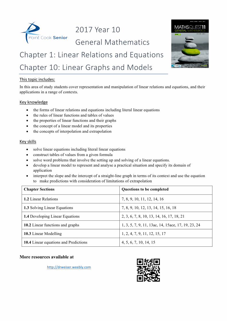
2017 Year 10 General Mathematics Chapter 1: Linear Relations and Equations Chapter 10: Linear Graphs and Models This topic includes: In this area of study students cover representation and manipulation of linear relations and equations, and their applications in a range of contexts. Key knowledge • the forms of linear relations and equations including literal linear equations • the rules of linear functions and tables of values • the properties of linear functions and their graphs • the concept of a linear model and its properties • the concepts of interpolation and extrapolation Key skills • solve linear equations including literal linear equations • construct tables of values from a given formula • solve word problems that involve the setting up and solving of a linear equations. • develop a linear model to represent and analyse a practical situation and specify its domain of application • interpret the slope and the intercept of a straight-line graph in terms of its context and use the equation to make predictions with consideration of limitations of extrapolation Chapter Sections Questions to be completed 1.2 Linear Relations 7, 8, 9, 10, 11, 12, 14, 16 1.3 Solving Linear Equations 7, 8, 9, 10, 12, 13, 14, 15, 16, 18 1.4 Developing Linear Equations 2, 3, 6, 7, 8, 10, 13, 14, 16, 17, 18, 21 10.2 Linear functions and graphs 1, 3, 5, 7, 9, 11, 13ac, 14, 15ace, 17, 19, 23, 24 10.3 Linear Modelling 1, 2, 4, 7, 9, 11, 12, 15, 17 10.4 Linear equations and Predictions 4, 5, 6, 7, 10, 14, 15 More resources available at http://drweiser.weebly.com
Transcript of 2017Year%10% General%Mathematics% Chapter%1:%Linear ... · GENERAL MATHEMATICS 2017 Page 6 of 20...
2017 Year 10 General Mathematics
Chapter 1: Linear Relations and Equations Chapter 10: Linear Graphs and Models This topic includes: In this area of study students cover representation and manipulation of linear relations and equations, and their applications in a range of contexts.
Key knowledge
• the forms of linear relations and equations including literal linear equations • the rules of linear functions and tables of values • the properties of linear functions and their graphs • the concept of a linear model and its properties • the concepts of interpolation and extrapolation
Key skills
• solve linear equations including literal linear equations • construct tables of values from a given formula • solve word problems that involve the setting up and solving of a linear equations. • develop a linear model to represent and analyse a practical situation and specify its domain of
application • interpret the slope and the intercept of a straight-line graph in terms of its context and use the equation
to make predictions with consideration of limitations of extrapolation
Chapter Sections Questions to be completed
1.2 Linear Relations 7, 8, 9, 10, 11, 12, 14, 16
1.3 Solving Linear Equations 7, 8, 9, 10, 12, 13, 14, 15, 16, 18
1.4 Developing Linear Equations 2, 3, 6, 7, 8, 10, 13, 14, 16, 17, 18, 21
10.2 Linear functions and graphs 1, 3, 5, 7, 9, 11, 13ac, 14, 15ace, 17, 19, 23, 24
10.3 Linear Modelling 1, 2, 4, 7, 9, 11, 12, 15, 17
10.4 Linear equations and Predictions 4, 5, 6, 7, 10, 14, 15
More resources available at
http://drweiser.weebly.com
GENERAL MATHEMATICS 2017
Page 2 of 20
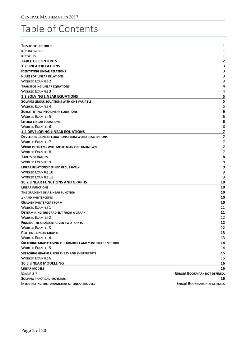
Table of Contents THIS TOPIC INCLUDES: 1 KEY KNOWLEDGE 1 KEY SKILLS 1 TABLE OF CONTENTS 2 1.2 LINEAR RELATIONS 3 IDENTIFYING LINEAR RELATIONS 3 RULES FOR LINEAR RELATIONS 3 WORKED EXAMPLE 2 3 TRANSPOSING LINEAR EQUATIONS 4 WORKED EXAMPLE 3 4 1.3 SOLVING LINEAR EQUATIONS 5 SOLVING LINEAR EQUATIONS WITH ONE VARIABLE 5 WORKED EXAMPLE 4 5 SUBSTITUTING INTO LINEAR EQUATIONS 6 WORKED EXAMPLE 5 6 LITERAL LINEAR EQUATIONS 6 WORKED EXAMPLE 6 6 1.4 DEVELOPING LINEAR EQUATIONS 7 DEVELOPING LINEAR EQUATIONS FROM WORD DESCRIPTIONS 7 WORKED EXAMPLE 7 7 WORD PROBLEMS WITH MORE THAN ONE UNKNOWN 7 WORKED EXAMPLE 8 7 TABLES OF VALUES 8 WORKED EXAMPLE 9 8 LINEAR RELATIONS DEFINED RECURSIVELY 9 WORKED EXAMPLE 10 9 WORKED EXAMPLE 11 9 10.2 LINEAR FUNCTIONS AND GRAPHS 10 LINEAR FUNCTIONS 10 THE GRADIENT OF A LINEAR FUNCTION 10 𝑥-‐ AND 𝑦-‐INTERCEPTS 10 GRADIENT–INTERCEPT FORM 10 WORKED EXAMPLE 1 11 DETERMINING THE GRADIENT FROM A GRAPH 11 WORKED EXAMPLE 2 12 FINDING THE GRADIENT GIVEN TWO POINTS 12 WORKED EXAMPLE 3 12 PLOTTING LINEAR GRAPHS 13 WORKED EXAMPLE 4 13 SKETCHING GRAPHS USING THE GRADIENT AND Y-‐INTERCEPT METHOD 14 WORKED EXAMPLE 5 14 SKETCHING GRAPHS USING THE X-‐ AND Y-‐INTERCEPTS 15 WORKED EXAMPLE 6 15 10.3 LINEAR MODELLING 16 LINEAR MODELS 16 EXAMPLE 7 ERROR! BOOKMARK NOT DEFINED. SOLVING PRACTICAL PROBLEMS 16 INTERPRETING THE PARAMETERS OF LINEAR MODELS ERROR! BOOKMARK NOT DEFINED.

LINEAR EQUATIONS, GRAPHS AND MODELS
Page 3 of 20
1.2 Linear Relations Identifying linear relations
A linear relation is a relationship between two variables that when plotted gives a straight line. Many real-life situations can be described by linear relations, such as water being added to a tank at a constant rate, or money being saved when the same amount of money is deposited into a bank at regular time intervals.
Rules for linear relations
Rules define or describe relationships between two or more variables. Rules for linear relations can be found by determining the common difference between consecutive terms of the pattern formed by the rule.
Consider the number pattern 3, 6, 9 and 12. This pattern is formed by adding 3 (the common difference is 3). If each number in the pattern is assigned a term number as shown in the table, then the expression to represent the common difference is 3𝑛 (i.e. 3 × 𝑛).
n 1 2 3 4
3n 3 6 9 12
So, the rule for this number pattern is 3𝑛.
Now, consider the number pattern 4, 7, 10 and 13. This pattern is also formed by adding 3. But it has a starting value of 4 not 3 so the rule for this number pattern is 3𝑛 + 1
If a rule has an equals sign, it is described as an equation. For example, 3𝑛 + 1 is referred to as an expression, but if we define the term number as 𝑡, then 𝑡 = 3𝑛 + 1 is an equation.
Worked Example 2
Find the equations for the linear relations formed by the following number patterns.
a) 3, 7, 11, 15
b) 8, 5, 2, −1

GENERAL MATHEMATICS 2017
Page 4 of 20
Note: It is good practice to substitute a second term number into your equation to check that your answer is correct.
Transposing linear equations
If we are given a linear equation between two variables, we are able to transpose (re-arrange) this relationship to express it in terms of either variable. That is, we can change the equation so that the variable on the right-hand side of the equation becomes the stand-alone variable on the left-hand side of the equation.
Worked Example 3
Transpose the linear equation 𝑦 = 4𝑥 + 7 to make 𝑥 the subject of the equation.
On the CAS
On a blank calculator page
c11 (remember we use documents, never scratchpad)
Type:
solve(𝑦 = 4×𝑥 + 7, 𝑥)
Press ·, the answer will be shown. The top one is if the calculator is set to “approximate” and the bottom “exact” or “auto”
To change this, c52, calculation mode (5th one down)

LINEAR EQUATIONS, GRAPHS AND MODELS
Page 5 of 20
1.3 Solving linear equations Solving linear equations with one variable
To solve linear equations with one variable, all operations performed on the variable need to be identified in order, and then the opposite operations need to be performed in reverse order.
In practical problems, solving linear equations can answer everyday questions such as the time required to have a certain amount in the bank, the time taken to travel a certain distance, or the number of participants needed to raise a certain amount of money for charity.
Worked Example 4
Solve the following linear equations to find the unknowns.
a) 5𝑥 = 12 b) 8𝑡 + 11 = 20 c) 12 = 4(𝑛-‐‑3) d) :;<=>
= 5
On the CAS Worked Example 4(c) and 4(d)
On a blank calculator page
c11 (remember we use documents, never scratchpad)
Type:
solve(12 = 4(𝑛 − 3), 𝑛) then press ·
solve(:;<=>
= 5, 𝑥) then press ·
GENERAL MATHEMATICS 2017
Page 6 of 20
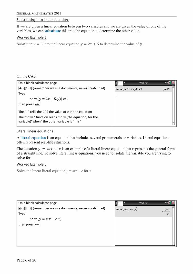
Substituting into linear equations
If we are given a linear equation between two variables and we are given the value of one of the variables, we can substitute this into the equation to determine the other value.
Worked Example 5
Substitute 𝑥 = 3 into the linear equation 𝑦 = 2𝑥 + 5 to determine the value of 𝑦.
On the CAS On a blank calculator page c11 (remember we use documents, never scratchpad) Type:
solve(𝑦 = 2𝑥 + 5, 𝑦)|x=3 then press ·
The “|” tells the CAS the value of 𝑥 in the equation The “solve” function reads “solve(the equation, for the variable)”when” the other variable is “this”
Literal linear equations
A literal equation is an equation that includes several pronumerals or variables. Literal equations often represent real-life situations.
The equation 𝑦 = 𝑚𝑥 + 𝑐 is an example of a literal linear equation that represents the general form of a straight line. To solve literal linear equations, you need to isolate the variable you are trying to solve for.
Worked Example 6
Solve the linear literal equation y = mx + c for x.
On a blank calculator page c11 (remember we use documents, never scratchpad) Type:
solve(𝑦 = 𝑚𝑥 + 𝑐, 𝑥) then press ·

LINEAR EQUATIONS, GRAPHS AND MODELS
Page 7 of 20
1.4 Developing linear equations Developing linear equations from word descriptions
To write a worded statement as a linear equation, we must first identifythe unknown and choose a pronumeral to represent it. We can then use the information given in the statement to write a linear equation in terms of the pronumeral.
The linear equation can then be solved as before, and we can use the result to answer the original question.
Worked Example 7
Cans of soft drinks are sold at SupaSave in packs of 12 costing $5.40. Form and solve a linear equation to determine the price of 1 can of soft drink.
Word problems with more than one unknown
In some instances, a word problem might contain more than one unknown. If we can express both unknowns in terms of the same pronumeral, we can create a linear equation as before and solve it to determine the value of both unknowns.
Worked Example 8
Georgina is counting the numberof insects and spiders, she can find in her back garden. All insects have6 legs and all spiders have 8 legs. In total, Georgina finds 43 bugs with a total of 290 legs. Form a linear equation to determine exactly how many insects and spiders Georgina found.
GENERAL MATHEMATICS 2017
Page 8 of 20
Tables of values
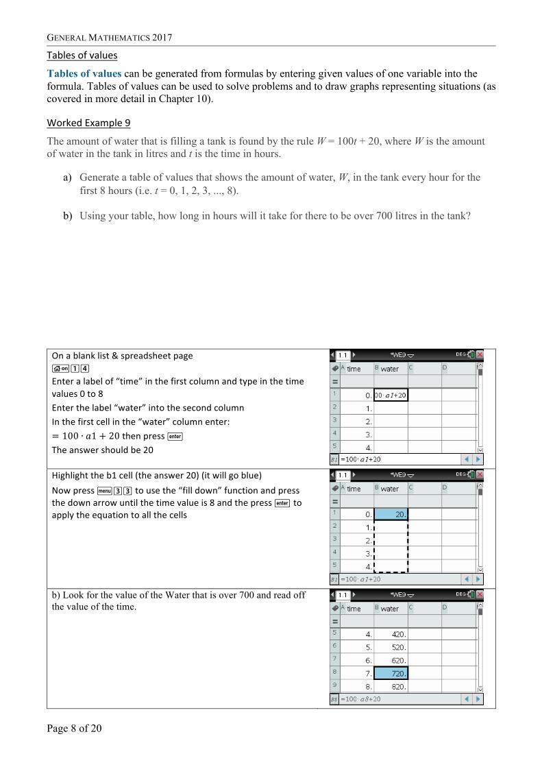
Tables of values can be generated from formulas by entering given values of one variable into the formula. Tables of values can be used to solve problems and to draw graphs representing situations (as covered in more detail in Chapter 10).
Worked Example 9
The amount of water that is filling a tank is found by the rule W = 100t + 20, where W is the amount of water in the tank in litres and t is the time in hours.
a) Generate a table of values that shows the amount of water, W, in the tank every hour for the first 8 hours (i.e. t = 0, 1, 2, 3, ..., 8).
b) Using your table, how long in hours will it take for there to be over 700 litres in the tank?
On a blank list & spreadsheet page c14 Enter a label of “time” in the first column and type in the time values 0 to 8 Enter the label “water” into the second column In the first cell in the “water” column enter: = 100 ∙ 𝑎1 + 20 then press · The answer should be 20
Highlight the b1 cell (the answer 20) (it will go blue) Now press b33 to use the “fill down” function and press the down arrow until the time value is 8 and the press · to apply the equation to all the cells
b) Look for the value of the Water that is over 700 and read off the value of the time.
LINEAR EQUATIONS, GRAPHS AND MODELS
Page 9 of 20
Linear relations defined recursively
Many sequences of numbers are obtained by following rules that define a relationship between any one term and the previous term. Such a relationship is known as a recurrence relation.
A term in such a sequence is defined as tn, with n denoting the place in the sequence. The term tn − 1 is the previous term in the sequence.
Worked Example 10 A linear recurrence relation is given by the formula 𝑡𝑛 = 𝑡𝑛
-‐‑
1 + 6, 𝑡1
= 5. Write the first six terms of the sequence.
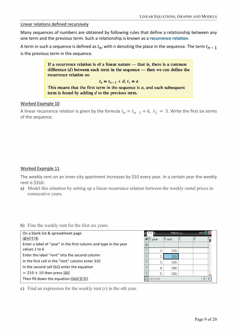
Worked Example 11
The weekly rent on an inner-‐city apartment increases by $10 every year. In a certain year the weekly rent is $310. a) Model this situation by setting up a linear recurrence relation between the weekly rental prices in
consecutive years.
b) Fine the weekly rent for the first six years. On a blank list & spreadsheet page c14 Enter a label of “year” in the first column and type in the year values 1 to 6 Enter the label “rent” into the second column In the first cell in the “rent” column enter 310 In the second cell (b2) enter the equation = 310 + 10 then press · Then fill down the equation (b33)
c) Find an expression for the weekly rent (r) in the nth year.
GENERAL MATHEMATICS 2017
Page 10 of 20
10.2 Linear functions and graphs Linear functions
A function is a relationship between a set of inputs and outputs, such that each input is related to exactly one output. A function of 𝑥 is denoted as 𝑓(𝑥). Each input and output can be expressed as an ordered pair, i.e. (𝑥, 𝑓(𝑥)) where 𝑥 is the input and 𝑓(𝑥) the output. A linear function is a set of ordered pairs that form a straight line when graphed.
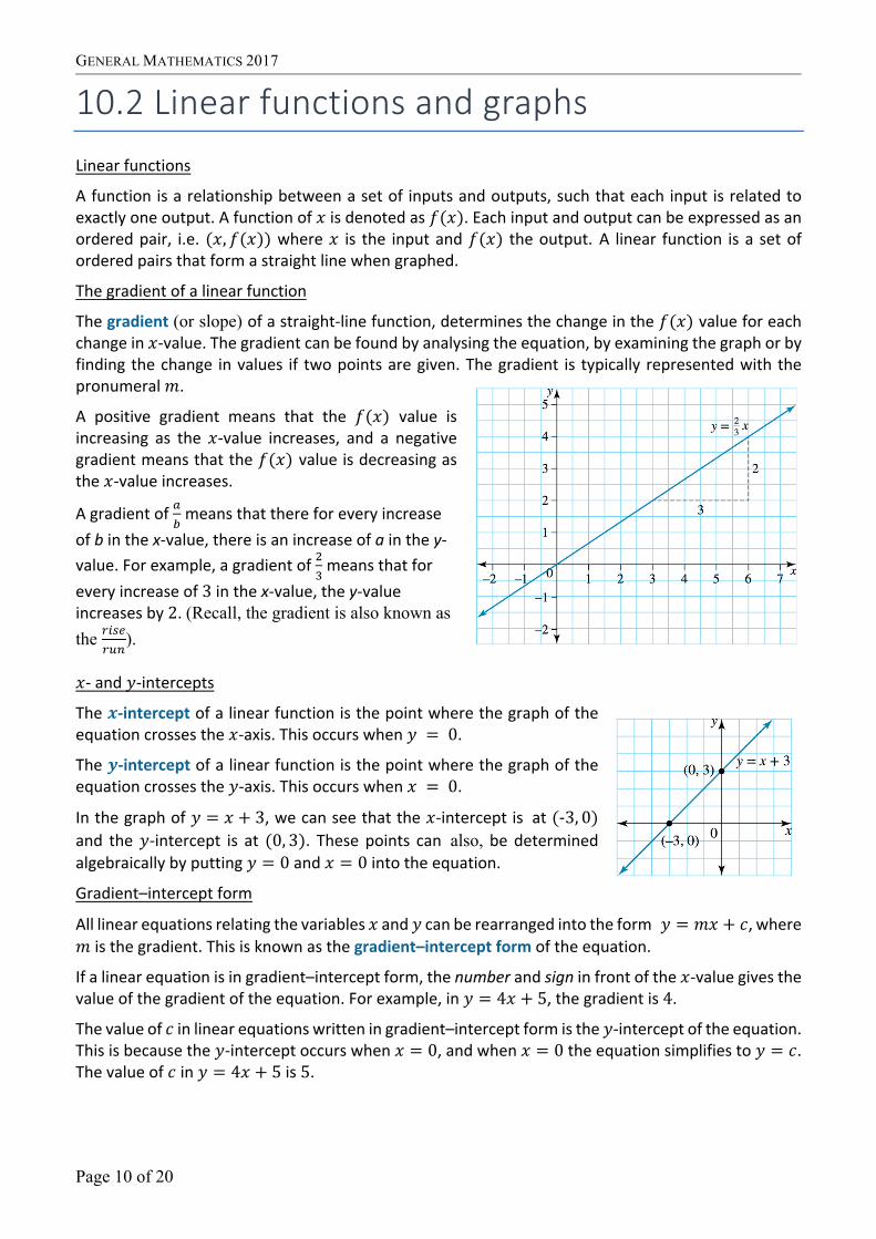
The gradient of a linear function
The gradient (or slope) of a straight-‐line function, determines the change in the 𝑓(𝑥) value for each change in 𝑥-‐value. The gradient can be found by analysing the equation, by examining the graph or by finding the change in values if two points are given. The gradient is typically represented with the pronumeral 𝑚.
A positive gradient means that the 𝑓(𝑥) value is increasing as the 𝑥-‐value increases, and a negative gradient means that the 𝑓(𝑥) value is decreasing as the 𝑥-‐value increases.
A gradient of EF means that there for every increase
of b in the x-‐value, there is an increase of a in the y-‐value. For example, a gradient of =
> means that for
every increase of 3 in the x-‐value, the y-‐value increases by 2. (Recall, the gradient is also known as the GHIJ
GKL).
𝑥-‐ and 𝑦-‐intercepts
The 𝒙-‐intercept of a linear function is the point where the graph of the equation crosses the 𝑥-‐axis. This occurs when 𝑦 = 0.
The 𝒚-‐intercept of a linear function is the point where the graph of the equation crosses the 𝑦-‐axis. This occurs when 𝑥 = 0.
In the graph of 𝑦 = 𝑥 + 3, we can see that the 𝑥-‐intercept isat (-‐‑3, 0) and the 𝑦-‐intercept is at (0, 3). These points canalso, be determined algebraically by putting 𝑦 = 0 and 𝑥 = 0 into the equation.
Gradient–intercept form
All linear equations relating the variables 𝑥 and 𝑦 can be rearranged into the form𝑦 = 𝑚𝑥 + 𝑐, where 𝑚 is the gradient. This is known as the gradient–intercept form of the equation.
If a linear equation is in gradient–intercept form, the number and sign in front of the 𝑥-‐value gives the value of the gradient of the equation. For example, in 𝑦 = 4𝑥 + 5, the gradient is 4.
The value of 𝑐 in linear equations written in gradient–intercept form is the 𝑦-‐intercept of the equation. This is because the 𝑦-‐intercept occurs when 𝑥 = 0, and when 𝑥 = 0 the equation simplifies to 𝑦 = 𝑐. The value of 𝑐 in 𝑦 = 4𝑥 + 5 is 5.

LINEAR EQUATIONS, GRAPHS AND MODELS
Page 11 of 20
Worked Example 1
State the gradients and y-‐intercepts of the following linear equations.
a) 𝑦 = 5𝑥 + 2
b) 2𝑦 = 4𝑥-‐‑6
On a blank calculator page c11
solve(2𝑦 = 4𝑥 − 6, 𝑦) then press ·
so the gradient is 2 and the y-‐intercept is −3
Determining the gradient from a graph
The value of the gradient can be found from a graph of a linear function. The gradient can be found by selecting two points on the line, then finding the change in the 𝑦-‐values and dividing by the change in the 𝑥-‐values.
In other words, the general rule to find the value of a gradient that passes through the points (𝑥1, 𝑦1) and (𝑥2, 𝑦2) is:
For all horizontal lines the 𝑦-‐values will be equal, so the numerator of OP<OQ;P<;Q
will be 0. Therefore, the gradient of vertical lines is 0.
For all vertical lines the 𝑥-‐values will be equal, so the denominator of OP<OQ;P<;Q
will be 0. Dividing a value by 0 is undefined; therefore, the gradient of vertical lines is undefined.

GENERAL MATHEMATICS 2017
Page 12 of 20
Worked Example 2
Find the values of the gradients of the following graphs.
a) b)
Finding the gradient given two points
If a graph is not provided, we can still find the gradient if we are given two points that the line passes through. The same formula is used to find the gradient by finding the difference in the two 𝑦-‐coordinates and the difference in the two 𝑥-‐coordinates:
For example, the gradient of the line that passes through the points (1, 1) and (4, 3) is
𝑚 =𝑦= − 𝑦R𝑥= − 𝑥R
=3 − 14 − 1 =
23
Worked Example 3
Find the value of the gradients of the linear graphs that pass through the following points.
a) (4,6) and (5,9)
b) (2, -‐‑1) and (0,5)
LINEAR EQUATIONS, GRAPHS AND MODELS
Page 13 of 20
Plotting linear graphs
Linear graphs can be constructed by plotting the points and then ruling a line between the points as shown in the diagram.
If the points or a table of values are not given, then the points can be found by substituting x-‐values into the rule and finding the corresponding y-‐values. If a table of values is provided, then the graph can be constructed by plotting the points given and joining them.
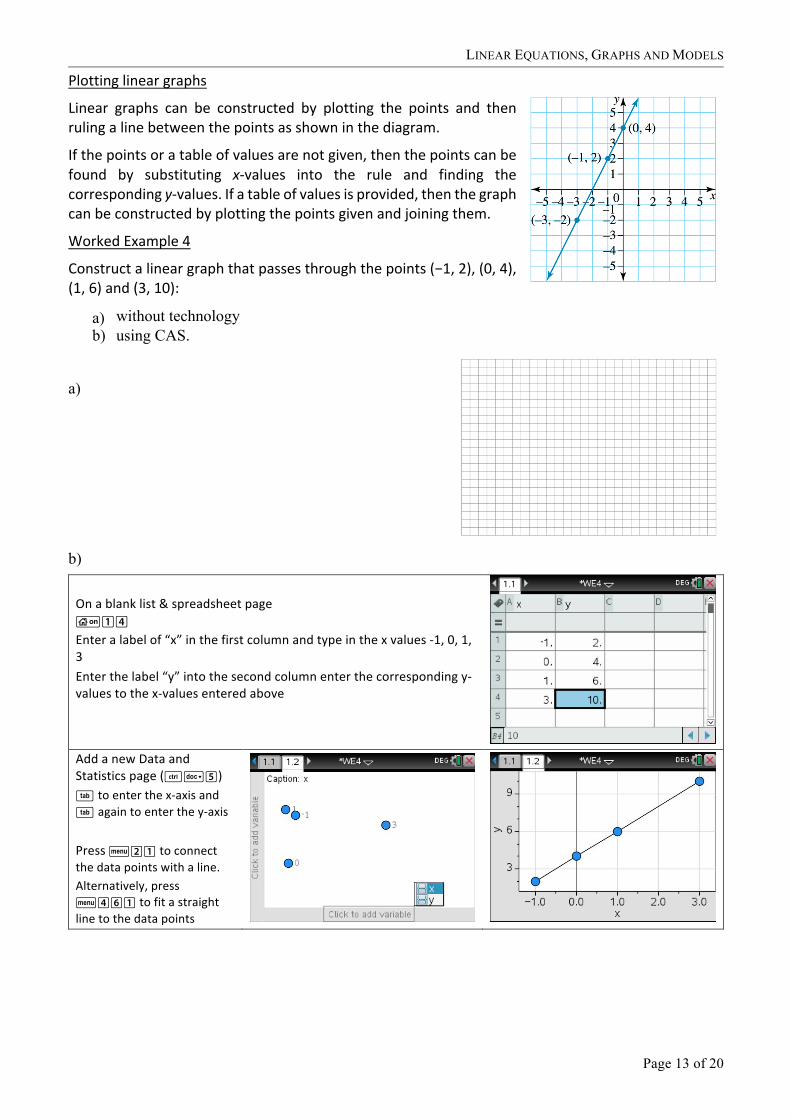
Worked Example 4
Construct a linear graph that passes through the points (−1, 2), (0, 4), (1, 6) and (3, 10):
a) without technology b) using CAS.
a)
b)
On a blank list & spreadsheet page c14 Enter a label of “x” in the first column and type in the x values -‐1, 0, 1, 3 Enter the label “y” into the second column enter the corresponding y-‐values to the x-‐values entered above
Add a new Data and Statistics page (/~5) e to enter the x-‐axis and e again to enter the y-‐axis Press b21 to connect the data points with a line. Alternatively, press b461 to fit a straight line to the data points

GENERAL MATHEMATICS 2017
Page 14 of 20
Sketching graphs using the gradient and y-‐intercept method
A linear graph can be constructed by using the gradient and y-‐intercept. The y-‐intercept is marked on the y-‐axis, and then another point is found by using the gradient.
Worked Example 5
Using the gradient and the y-‐intercept, sketch the graph of each of the following.
a) 𝑦 = >:𝑥 − 2
b) A linear graph with a gradient of 3 and a y-intercept of 1
c) y=−2x+4
LINEAR EQUATIONS, GRAPHS AND MODELS
Page 15 of 20
Sketching graphs using the x-‐ and y-‐intercepts
If the points of a linear graph where theline crosses the 𝑥-‐ and 𝑦-‐axes (the 𝑥-‐ and 𝑦-‐intercepts) are known, then the graph can be constructed by marking these points and ruling a line through them.
To find the 𝑥-‐intercept, substitute 𝑦 = 0 into the equation and then solve the equation for 𝑥.
To find the 𝑦-‐intercept, substitute 𝑥 = 0 into the equation and then solve the equation for 𝑦.
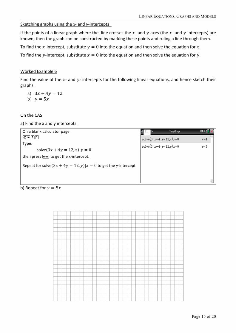
Worked Example 6
Find the value of the 𝑥-‐ and 𝑦-‐ intercepts for the following linear equations, and hence sketch their graphs.
a) 3𝑥 + 4𝑦 = 12 b) 𝑦 = 5𝑥
On the CAS
a) Find the x and y intercepts.
On a blank calculator page c11 Type:
solve 3𝑥 + 4𝑦 = 12, 𝑥 |𝑦 = 0 then press · to get the x-‐intercept.
Repeat for solve 3𝑥 + 4𝑦 = 12, 𝑦 |𝑥 = 0 to get the y-‐intercept
b) Repeat for 𝑦 = 5𝑥
GENERAL MATHEMATICS 2017
Page 16 of 20
10.3 Linear modelling Linear models
Practical problems in which there is a constant change over time can be modelled by linear equations. The constant change, such as therate at which water is leaking or the hourly rate charged by a tradesperson, can be represented by the gradient of the equation.
Usually the 𝑦-‐value is the changing quantity and the 𝑥-‐value is time.
The starting point or initial point of the problemis represented by the y-‐intercept, when thex-‐value is 0. This represents the initial or startingvalue. In situations where there is a negativegradient the x-‐intercept represents when there is nothing left, such as the time taken for a leaking water tank to empty.
Identifying the constant change and the starting point can help to construct a linear equation to represent a practical problem. Once this equation has been established we can use it to calculate specific values or to make predictions as required.
Solving practical problems
Once an equation is found to represent the practical problem, solutions to the problem can be found. When we have determined important values in practical problems, such as the value of the intercepts and gradient, it is important to be able to relate these back to the problem and to interpret their meaning. Knowing the equation can also help to find other values related to the problem (at a certain time for example).
Example 8
A yoga ball is being pumped full of air at a rate of 40 cm3/second. Initially there is 100 cm3 of airin the ball.
a) Construct an equation that represents the amount of air, A, in the ball after t seconds.
b) Interpret what the value of the y-‐intercept in the equation means.
c) How much air, in cm3, is in the ball after 2 minutes?

LINEAR EQUATIONS, GRAPHS AND MODELS
Page 17 of 20
d) When fully inflated, the ball holds 100 000 cm3 of air. Determine how long, in minutes, it takes to fully inflate the ball. Write your answer to the nearest minute.
The domain of a linear model
When creating a linear model, it is important to interpret the given informationto determine the domain of the model, that is, the values for which the model is applicable.
The domains of linear models are usually expressed using the less than or equal to sign (≤) and the greater than or equal to sign (≥).
For example, in the previous example about air pumped into a yoga ball at a constant rate, the model will stop being valid before 100cm3 and after 100 000 cm3 of air is in the yoga ball, so the domain only includes x-‐values for when this is true.
Example 9
Express the following situations as linear models and give the domains of the models.
a) Julie works at a department store and is paid $19.20 per hour. She must work for a minimum of 10 hours per week, but due to her study commitments she can work for no more than 20 hours per week.
b) The results in a driving test are marked out of 100, with 4 marks taken off for every error made on the course. The lowest possible result is 40 marks.

GENERAL MATHEMATICS 2017
Page 18 of 20
10.4 Linear equations and predictions This section is presented from the linear equation perspective. We will cover this from a data and statistics perspective in Unit 2 – Statistics. Finding the equation of straight lines
Given the gradient and y-‐intercept
When we are given the gradient and 𝑦-‐intercept of a straight line, we can enter these values into the equation 𝑦 = 𝑚𝑥 + 𝑐 to determine the equation of the straight line. Remember that 𝑚 is equal to the value of the gradient and c is equal to the value of the 𝑦-‐intercept.
For example, if we are given a gradient of 3 and a 𝑦-‐intercept of 6, then the equation of the straight line would be 𝑦 = 3𝑥 + 6.
Given the gradient and one point
When we are given the gradient and one point of a straight line, we need to establish the value of the y-‐intercept to find the equation of the straight line. This can be done by substituting the coordinates of the given point into the equation 𝑦 = 𝑚𝑥 + 𝑐 and then solving for 𝑐. Remember that 𝑚 is equal to the value of the gradient, so this can also be substituted into the equation.
Given two points
When we are given two points of a straight line, we can find the value of thegradient of a straight line between these points as discussed in Section 10.2 (by using 𝑚 = OP<OQ
;P<;Q). Once the gradient is
found, we can find the 𝑦-‐intercept by substituting one of the points into the equation 𝑦 = 𝑚𝑥 + 𝑐 and then solving for 𝑐.
Example 10
Find the equations of the following straight lines.
a) A straight line with a gradient of 5 passing through the point (-‐‑2, -‐‑5)
b) A straight line passing through the points (-‐‑3, 4) and (1, 6)
c) A straight line passing through the points (-‐‑3, 7) and (0, 7)
LINEAR EQUATIONS, GRAPHS AND MODELS
Page 19 of 20
Lines of best fit by eye
Sometimes the data for a practical problem may not be in the form of a perfect linear relationship, but the data can still be modelled by an approximate linear relationship.
When we are given, a scatterplot representing data that appears to be approximately represented by a linear relationship, we can draw aline of best fit by eye so that approximately half of the data points are on either side of the line of best fit.
Lines of best fit by eye
Sometimes the data for a practical problem may not be in the form of a perfect linear relationship, but the data can still be modelled by an approximate linear relationship.
When we are given a scatterplot representing data that appears to be approximately represented by a linear relationship, we can draw aline of best fit by eye so that approximately half of the data points are on either side of the line of best fit.
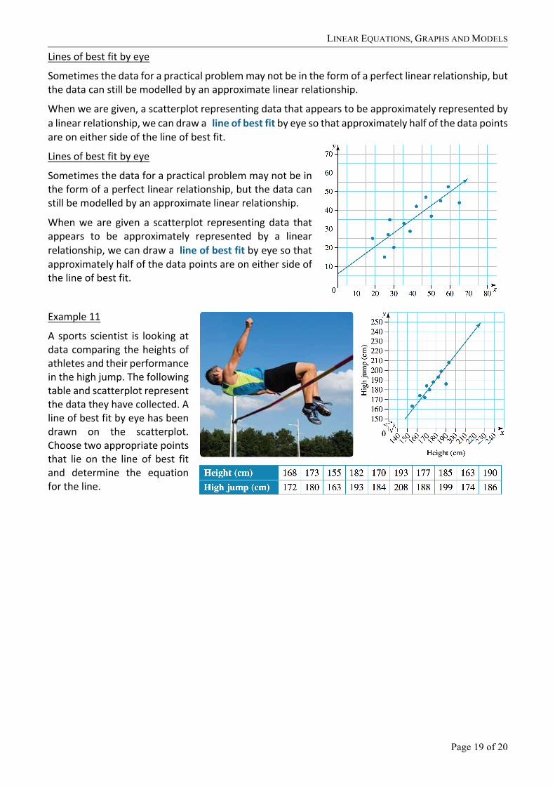
Example 11
A sports scientist is looking at data comparing the heights of athletes and their performance in the high jump. The following table and scatterplot represent the data they have collected. A line of best fit by eye has been drawn on the scatterplot. Choose two appropriate points that lie on the line of best fit and determine the equation for the line.
GENERAL MATHEMATICS 2017
Page 20 of 20
Making predictions
Interpolation
When we use interpolation, we aremaking a prediction from a line of bestfit that appears within the parameters ofthe original data set.
If we plot our line of best fit on the scatterplot of the given data, then interpolation will occur between thefirst and last points of the scatterplot.
Extrapolation
When we use extrapolation, we are making a prediction from a line of best fit that appears outside the parameters of the original data set.
Reliability of predictions
The more pieces of data there are in a set, the better the line of best fit you will be able to draw. More data points allow more reliable predictions.
In general, interpolation is a far more reliable method of making predictions than extrapolation. However, there are other factors that should also be considered. Interpolation closer to the centre of the data set will be more reliable that interpolation closer to the edge of the data set. Extrapolation that appears closer to the data set will be much more reliable than extrapolation that appears further away from the data set.
Worked Example 12
The following data represent the air temperature (°C) and depth of snow (cm) at a popular ski resort.
The line of best fit for this data set has been calculated as 𝑦 = -‐‑7.2𝑥 + 84.
a) Use the line of best fit to estimate the depth of snow if the air temperature is -‐‑6.5°𝐶.
b) Use the line of best fit to estimate the depth of snow if the air temperature is 25.2°𝐶.
c) Comment on the reliability of your estimations in parts a) and b).