2017 Report on Financial Condition and Economic Experience...
58
Office of the State Actuary “Supporting financial security for generations. ” 2017 Report on Financial Condition and Economic Experience Study PREPARED FOR THE PENSION FUNDING COUNCIL • AUGUST 2017
Transcript of 2017 Report on Financial Condition and Economic Experience...

Office of the State Actuary“Supporting financial security for generations.”
2017 Report on Financial Condition and Economic Experience Study
PREPARED FOR THE PENSION FUNDING COUNCIL • AUGUST 2017


To obtain a copy of this report in alternative format call 360.786.6140 or 711 for TDD.
Office of the State Actuary“Supporting financial security for generations.”
Mailing AddressOffice of the State Actuary PO Box 40914 Olympia, Washington 98504-0914
Physical Address2100 Evergreen Park Dr. SW
Suite 150
PhoneReception: 360.786.6140 TDD: 711 Fax: 360.586.8135
Electronic [email protected] leg.wa.gov/osa
Report PreparationMatthew M. Smith, FCA, EA, MAAAState Actuary
Sarah Baker
Kelly Burkhart
Mitch DeCamp
Graham Dyer
Aaron Gutierrez, MPA, JD
Beth Halverson
Michael Harbour, ASA, MAAA
Lisa Hawbaker
Luke Masselink, ASA, EA, MAAA
Corban Nemeth
Darren Painter
Stephanie Roman, MA, JD
Frank Serra
Christi Steele
Kyle Stineman, ASA
Keri Wallis
Lisa Won, ASA, FCA, MAAA
Additional AssistanceDepartment of Retirement SystemsPension Funding Council Work GroupWashington State Investment BoardLegislative Support Services


ContentsLetter of Introduction . . . . . . . . . . . . . . . . . . . . . . . . . . . . .V
SECTION ONE: REPORT ON FINANCIAL CONDITION . . . . . . . . . . . . . . . . . . . 1
Current Status of Retirement Systems . . . . . . . . . . . . . . . . 4
Where the Retirement Systems are Headed . . . . . . . . . . . . 9
How the Future Can Look Different . . . . . . . . . . . . . . . . . .11
How Can We Put the Systems in the Best Financial Condition for the Future . . . . . . . . . . . . . . .14
SECTION TWO: ECONOMIC EXPERIENCE STUDY . . . . . . . . . . . . . . . . . . . . . .17
Executive Summary . . . . . . . . . . . . . . . . . . . . . . . . . . . . .19
General Approach to Setting Economic Assumptions . . . . 20
Experience Study and Recommended Assumptions . . . . . 20
Total Inflation . . . . . . . . . . . . . . . . . . . . . . . . . . . . . . . . . .21
General Salary Growth . . . . . . . . . . . . . . . . . . . . . . . . . . 22
Investment Rate of Return . . . . . . . . . . . . . . . . . . . . . . . . 23
Growth in System Membership . . . . . . . . . . . . . . . . . . . . .24
Actuarial Certification Letter . . . . . . . . . . . . . . . . . . . . . . .25
SECTION THREE: ECONOMIC EXPERIENCE STUDY APPENDICES . . . . . . . . . . 27
APPENDIX A – Total Inflation Assumption . . . . . . . . . . . . . . . 29Methodology . . . . . . . . . . . . . . . . . . . . . . . . . . . . . . . . . . 29
Analysis . . . . . . . . . . . . . . . . . . . . . . . . . . . . . . . . . . . . . 29
Exhibits A . . . . . . . . . . . . . . . . . . . . . . . . . . . . . . . . . . . . .32
APPENDIX B – General Salary Growth Assumption . . . . . . . . 33Methodology . . . . . . . . . . . . . . . . . . . . . . . . . . . . . . . . . . 33
Analysis . . . . . . . . . . . . . . . . . . . . . . . . . . . . . . . . . . . . . 33
Exhibits B . . . . . . . . . . . . . . . . . . . . . . . . . . . . . . . . . . . . 36
APPENDIX C – Investment Rate Of Return Assumption . . . . . 37Methodology . . . . . . . . . . . . . . . . . . . . . . . . . . . . . . . . . . .37
Analysis . . . . . . . . . . . . . . . . . . . . . . . . . . . . . . . . . . . . . .37
Exhibits C . . . . . . . . . . . . . . . . . . . . . . . . . . . . . . . . . . . . 43
APPENDIX D – Growth In System Membership Assumption . . 45Methodology . . . . . . . . . . . . . . . . . . . . . . . . . . . . . . . . . . 45
Analysis . . . . . . . . . . . . . . . . . . . . . . . . . . . . . . . . . . . . . 45
Exhibits D . . . . . . . . . . . . . . . . . . . . . . . . . . . . . . . . . . . . 48


Letter of Introduction 2017 Report on Financial Condition
and Economic Experience Study
August 2017
As required under RCW 41.45.030, this report documents the results of a study on financial condition and long-term economic experience for the Washington State retirement systems performed by the Office of the State Actuary (OSA).
The primary purpose of this report is to assist the Pension Funding Council (PFC) in evaluating whether to adopt changes to the long-term economic assumptions identified in RCW 41.45.035. We do not recommend using this report for other purposes.
The focus of the Report on Financial Condition is on the financial health of the retirement systems, whereas the Economic Experience Study involves comparing actual economic experience with the assumptions made and considering future expectations for these assumptions. Pursuant to statute, the Economic Experience Study also includes a set of recommended long-term economic assumptions made by the State Actuary.
We encourage you to submit any questions you might have concerning this report to our regular address or our e-mail address at [email protected]. We also invite you to visit our website (leg.wa.gov/osa) for further information regarding the actuarial funding of the Washington State retirement systems.
Sincerely,
Matthew M. Smith, FCA, EA, MAAA Kyle Stineman, ASAState Actuary Senior Actuarial Analyst
PO Box 40914 | Olympia, Washington 98504-0914 | [email protected] | leg.wa.gov/osaPhone: 360.786.6140 | Fax: 360.586.8135 | TDD: 711
Office of the State Actuary“Supporting financial security for generations.”
LETTER OF INTRODUCTION


REPORT ON FINANCIAL CONDITION
SECTION ONE:

SECTION ONE: REPORT ON FINANCIAL CONDITION
2017 REPORT ON FINANCIAL CONDITION AND ECONOMIC EXPERIENCE STUDY 3
Report on Financial ConditionThe Report on Financial Condition (RFC) brings together key findings and themes from pension reports produced by the Office of the State Actuary (OSA). OSA is required under RCW 41.45.030 to provide information on the experience and financial condition of the retirement systems. We present this report and Economic Experience Study to assist the Pension Funding Council (PFC) in evaluating whether to adopt changes to the long-term economic assumptions identified in RCW 41.45.035.
We use both affordability and solvency measures to report on the financial condition (or health) of the Washington State retirement systems. For this report, we define affordability as the ability to provide adequate funding to the pension plans. Solvency is defined as the ability of the pension plans to pay for benefits earned by its members.
In this report, we present our assessment of the affordability and solvency of Washington State pension plans by reviewing both current and projected actuarial measures. We also consider how the affordability and solvency of the pension plans can change if future experience does not match our assumptions. The RFC is broken into the following sections:
Current Status of Retirement Systems, where we provide financial condition measures on a historical and current basis.
Where the Retirement Systems are Headed, including how the measures look based on our long-term expectations for the retirement systems.
How the Future Can Look Different, where we examine how the observed measures can change if experience does not match expectations.
To develop this report, we had to ask ourselves what measures best determine the financial health of the Washington State retirement systems. After careful consideration, we selected affordability and solvency as the best measures to answer this question because they address the cost to employees and employers as well as whether the plans can pay for the earned benefits of its members. We advise the reader to take into consideration affordability and solvency measures outlined in all three sections of this report before making a determination on the financial condition of the retirement systems. It is important to consider this report in its entirety because observed trends in one section may differ in another section.

4 2017 REPORT ON FINANCIAL CONDITION AND ECONOMIC EXPERIENCE STUDY
SECTION ONE: REPORT ON FINANCIAL CONDITION
Current Status of Retirement SystemsAdequate funding improves the health of the Washington State retirement systems. The adequate (or required) contributions represent the contributions necessary to satisfy full funding under current benefit provisions, assumptions, methods, and funding policy defined under Chapter 41.45, RCW.
OSA performs actuarial valuations annually on the Washington State retirement systems. OSA calculates the required contribution rates, as a percent of salary, necessary to fully fund the systems based on the adopted funding policy and long-term assumptions disclosed in the Actuarial Valuation Report (AVR). OSA presents the results to the PFC and Law Enforcement Officers’ and Fire Fighters’ Retirement System (LEOFF) Plan 2 Board. The PFC and LEOFF Plan 2 Board adopt contribution rates on a bi-annual basis, subject to revision by the Legislature. The adopted or enacted contribution rates may differ from the required contribution rates.
We assess the affordability of a pension system based on the ability to provide adequate contributions to fund the plan. It is helpful to review the biennial change in contribution rates in order to gauge the current affordability of a pension plan. The biennial change in contribution rates is important because the ability to provide adequate contributions may depend upon the budget set aside or available for pensions. The various budget pressures of the state can impact the budget for pensions. Budget writers, employers, and plan members can better plan and prepare for the financial resources needed to pay contributions if the future rates are predictable, particularly in the short-term, based on historical trends. The Legislature adopted an asset smoothing method in 2003 to help limit biennial volatility in contribution rates due to short-term asset returns that vary from long-term expectations.
The table below displays the adopted employee and employer contribution rates for the 2017-19 Biennium.
EmployeeSystem Normal Cost Normal Cost UAAL Total
PERS3 7.38% 7.49% 5.03% 12.52%TRS3 7.06% 7.83% 7.19% 15.02%SERS3 7.27% 8.27% 5.03% 13.30%PSERS 6.73% 6.73% 5.03% 11.76%LEOFF4 8.75% 8.75% 0.00% 8.75%WSPRS 7.34% 12.81% N/A 12.81%1 Excludes DRS administrative expense fee.2 Does not include supplemental rate impacts from 2017 Legislative Session.
Adopted 2017-19 Contribution Rates1
Employer2
3 Plan 1 members' contribution rate is statutorily set at 6.0%. Members in Plan 3 do not make contributions to their defined benefit.4 No member or employer contributions are required for LEOFF Plan 1 when the plan is fully funded.
SECTION ONE: REPORT ON FINANCIAL CONDITION
2017 REPORT ON FINANCIAL CONDITION AND ECONOMIC EXPERIENCE STUDY 5
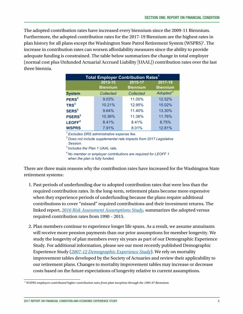
The adopted contribution rates have increased every biennium since the 2009-11 Biennium. Furthermore, the adopted contribution rates for the 2017-19 Biennium are the highest rates in plan history for all plans except the Washington State Patrol Retirement System (WSPRS)1. The increase in contribution rates can worsen affordability measures since the ability to provide adequate funding is constrained. The table below summarizes the change in total employer (normal cost plus Unfunded Actuarial Accrued Liability [UAAL]) contribution rates over the last three biennia.
There are three main reasons why the contribution rates have increased for the Washington State retirement systems:
1. Past periods of underfunding due to adopted contribution rates that were less than the required contribution rates. In the long-term, retirement plans become more expensive when they experience periods of underfunding because the plans require additional contributions to cover “missed” required contributions and their investment returns. The linked report, 2016 Risk Assessment Assumptions Study, summarizes the adopted versus required contribution rates from 1990 – 2015.
2. Plan members continue to experience longer life spans. As a result, we assume annuitants will receive more pension payments than our prior assumptions for member longevity. We study the longevity of plan members every six years as part of our Demographic Experience Study. For additional information, please see our most recently published Demographic Experience Study (2007-12 Demographic Experience Study). We rely on mortality improvement tables developed by the Society of Actuaries and review their applicability to our retirement plans. Changes to mortality improvement tables may increase or decrease costs based on the future expectations of longevity relative to current assumptions.
1 WSPRS employers contributed higher contribution rates from plan inception through the 1995-97 Biennium.
2013-15 Biennium
2015-17 Biennium
2017-19 Biennium
System Collected Collected Adopted 2
PERS3 9.03% 11.00% 12.52%TRS3 10.21% 12.95% 15.02%SERS3 9.64% 11.40% 13.30%PSERS3 10.36% 11.36% 11.76%LEOFF4 8.41% 8.41% 8.75%WSPRS 7.91% 8.01% 12.81%1 Excludes DRS administrative expense fee.
3 Includes the Plan 1 UAAL rate.4 No member or employer contributions are required for LEOFF 1 when the plan is fully funded.
Total Employer Contribution Rates1
2 Does not include supplemental rate impacts from 2017 Legislative Session.

6 2017 REPORT ON FINANCIAL CONDITION AND ECONOMIC EXPERIENCE STUDY
SECTION ONE: REPORT ON FINANCIAL CONDITION
3. The expectations for future return on investments have decreased. In general, employee/employer contributions funded approximately 25-30 percent of the cost of the Washington State retirement systems over the past 20 years. Investment returns generated on contributions funded approximately 70-75 percent of the cost. Contributions would now need to increase to offset the expected decrease in future investment returns. We analyze our investment return recommendation as part of the Economic Experience Study every two years.
The annual change in contribution rates, however, is not the only measure to determine the affordability of the Washington State retirement systems. Contributions as a percent of budget and plan maturity measures will also help in determining affordability.
A trend that shows consistent increases in the contributions, as a percent of budget, might suggest the plans have become less affordable. The table below summarizes the estimated General Fund-State (GF-S) pension contributions as a percent of the GF-S Budget.
(Dollars in Millions) 1990 1994 2000 2005 2010 2015 2016Estimated GF-S Contributions* $222 $323 $265 $81 $384 $639 $796GF-S Budget** $6,505 $8,013 $11,068 $13,036 $13,571 $17,283 $18,579Percent of GF-S Budget 3.4% 4.0% 2.4% 0.6% 2.8% 3.7% 4.3%*Actual total employer contributions found in the 1995, 2005, 2009, and 2014 OFM CAFRs. The estimated GF-S contributions is the product of actual employer contributions and assumed GF-S fund splits (found on OSA's website).**GF-S budgets prior to 1997 found in June 2008 ERFC Annual Forecast. All other GF-S budgets found in June 2017 ERFC Annual Forecast.
Estimated Pension Contributions as a Percent of GF-S Budget
In general, we observe the displayed percentages trend downwards from Fiscal Year (FY) 1990 to FY 2005 and trend upwards following FY 2005. Please see the 2010 Risk Assessment Study for information on why this occurred. As of the most recent valuation, the highest estimated GF-S pension contributions as a percent of GF-S budget occurred in FY 2016 (4.3 percent), coinciding with the highest collected contribution rates. Looking forward, we believe it is reasonable to assume that the state can maintain pension contributions up to levels provided in the table because the state met these levels in the past.
The table above provides information on what the state could afford in the past but we also consider who pays for these pension contributions. Active employees and their employers contribute to the Washington State retirement systems. The contributions, and investment returns on contributions, fund the expected benefits of the systems. As the retirement systems mature, there are fewer active members resulting in employers assuming a larger share of future pension costs/funding. The reduction in the ratio of active members to retirees indicates more pressure on contributing members and their employers. The table below shows the maturity measures of the Washington State retirement systems.
2006 2008 2010 2012 2014Ratio of Actives to Retirees 2.4 2.4 2.2 2.0 1.9Liability Ratio: Retiree/Total 0.4 0.4 0.4 0.4 0.4
Select Plan Maturity Measures (All Plans Combined)

SECTION ONE: REPORT ON FINANCIAL CONDITION
2017 REPORT ON FINANCIAL CONDITION AND ECONOMIC EXPERIENCE STUDY 7
The ratio of actives to retirees has trended downward since FY 2006. We observed approximately 0.50 fewer actives per retirees over an eight-year period. Furthermore, we observe retirees have become a larger portion of total liabilities due to a trend of fewer actives per retiree. These trends have emerged because Plan 1 systems are now primarily comprised of annuitants and retirees are beginning to emerge from Plans 2/3.
Consistent with the state’s funding policy and goals, OSA calculates the contribution rates necessary to fully fund the pension system. Contribution rates measure the cost of the pension system as of a point in time and are intended to fund each year of future service accruals plus any unfunded past service costs consistent with the state’s funding policy. To get a broader picture of plan health it is important to also understand how the past funding has evolved. This can be done by calculating the funded ratio of the plan and reviewing a consistent measurement over time. The funded ratio takes into account the cumulative effect of past funding and benefits earned by members.
OSA uses the funded ratio as a solvency measure in this report. The funded ratio represents a commonly used measure of plan health that readers can use to assess the question “has the plan accumulated sufficient assets to pay the expected benefits that have been earned to date by its members?” A funded ratio, also known as funded status, is a measurement calculated at a specific point in time that assumes all actuarial assumptions will be fully realized. To determine the funded status, the value of plan assets are divided by the present value of all accrued (or earned) benefits of the plan. For example, if the funded status of a plan is 103 percent, then we assume there is $1.03 in assets for every $1.00 of present value of accrued (or earned) benefits. For these calculations, we use the long-term expected rate of return consistent with the state’s funding policy to determine the present value of accrued benefits.
While it is convenient to compare and report a funded status for the combined plans, we need to look at each plan independently. Absent a qualified merger or plan termination, plans cannot use another plan’s assets to pay its benefits. The following graph shows the funded status, by plan, as of our most recently published AVR.
58%
88%
64%
92% 89%95%
125%
105%98%
86%
40%
60%
80%
100%
120%
140%
PERS 1 PERS 2/3 TRS 1 TRS 2/3 SERS 2/3 PSERS 2 LEOFF 1 LEOFF 2 WSPRS 1/2 Total
Funded Status as of June 30, 2015
8 2017 REPORT ON FINANCIAL CONDITION AND ECONOMIC EXPERIENCE STUDY
SECTION ONE: REPORT ON FINANCIAL CONDITION
The actuarial community has not agreed on a funded status threshold that determines a plan as “healthy”; however, we consider all open plans as well as LEOFF Plan 1 on target for full funding. As of the latest measurements, the Public Employees’ Retirement System (PERS) Plan 1 and Teachers’ Retirement System (TRS) Plan 1 have a sizable mismatch between the plan’s estimated accrued (or earned) obligations and assets. For this reason, PERS 1 and TRS 1 require additional contributions in order to get their funding levels back on track for full funding. As defined under RCW 41.45.060, only employers make the additional contributions to PERS 1 and TRS 1.
The funded status is a point-in-time measurement. The goal is to reach a funded status of 100 percent, but future events are unknown and can influence the funded status of a plan. A review of the historical funded status provides information on the funding progress of each plan. The link to the 2014 AVR will summarize the funded status from 1986 to 2014. The 2014 AVR summarizes the funded status under the Projected Unit Credit (PUC) actuarial cost method. As of our 2015 AVR, the funded status is calculated using the Entry Age Normal (EAN) actuarial cost method consistent with Governmental Accounting Standards Board (GASB) requirements 67/68. The funded status will vary depending upon the asset valuation and actuarial cost methods used. Thus, we see a blip in the historical review when the cost method used for the funded status measure switched from PUC to EAN. However, when we take the shift in actuarial costs method into account, we still observe the funded status has generally decreased over the years. This is attributable to OSA recognizing increased life spans, lower assumed future investment returns, and periods of underfunding in our calculation of the funded status of Washington retirement systems. The decrease in the funded status for the open plans is also attributable to the maturing of those plans. Even without the factors noted above, we would expect the funded status of the opens plans to converge to 100 percent as the plans evolved from new, smaller plans to their more mature, current status. Despite the decreasing funded status for the plans, we believe all open plans and LEOFF 1 remain on target for full funding. The closed PERS 1 and TRS 1 require additional contributions in order to achieve full funding. The additional contributions are already included in the current plan 1 funding policy.
In summation, we observe the selected affordability and solvency measures worsening over the historical period. The plan affordability has trended downward partially due to an increase in contribution rates. This increase in contribution rates can make it more difficult to provide adequate funding due to pensions becoming a larger part of the budget. Furthermore, the estimated GF-S pension contributions as a percent of GF-S budget has increased each year since 2005. Lastly, the retirement systems are maturing, which means relatively fewer active members to retirees fund the retirement benefits. The solvency measure we selected for this report, funded status, has trended downward; however, we believe all open plans and LEOFF 1 remain on target for full funding. Consistent with current funding policy the closed PERS 1 and TRS 1 require additional contributions in order to achieve full funding. As noted in the next section of this report, if those future contributions are made consistent with current funding policy, we expect those plans to reach full funding in the future.
SECTION ONE: REPORT ON FINANCIAL CONDITION
2017 REPORT ON FINANCIAL CONDITION AND ECONOMIC EXPERIENCE STUDY 9
Where the Retirement Systems are HeadedThe Current Status of Retirement Systems section provides context on where our select affordability and solvency measures have been; however, it is also helpful to consider the expected affordability and solvency measures moving forward. We project future affordability and solvency measures because measurement trends observed in the past may change in the future. In addition, pension provisions in Washington State are generally considered contractual rights for current members. It is important to review the projected health of the plans because it may not be possible to reduce contractual benefits in the future if the health of the plan declines.
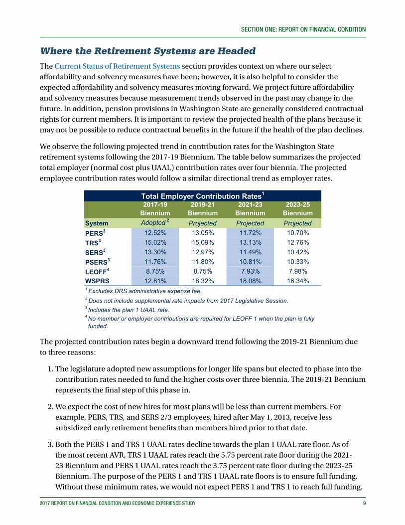
We observe the following projected trend in contribution rates for the Washington State retirement systems following the 2017-19 Biennium. The table below summarizes the projected total employer (normal cost plus UAAL) contribution rates over four biennia. The projected employee contribution rates would follow a similar directional trend as employer rates.
2017-19 Biennium
2019-21 Biennium
2021-23 Biennium
2023-25 Biennium
System Adopted 2 Projected Projected ProjectedPERS3 12.52% 13.05% 11.72% 10.70%TRS3 15.02% 15.09% 13.13% 12.76%SERS3 13.30% 12.97% 11.49% 10.42%PSERS3 11.76% 11.80% 10.81% 10.33%LEOFF4 8.75% 8.75% 7.93% 7.98%WSPRS 12.81% 18.32% 18.08% 16.34%1 Excludes DRS administrative expense fee.2 Does not include supplemental rate impacts from 2017 Legislative Session.
Total Employer Contribution Rates1
4 No member or employer contributions are required for LEOFF 1 when the plan is fully funded.
3 Includes the plan 1 UAAL rate.
The projected contribution rates begin a downward trend following the 2019-21 Biennium due to three reasons:
1. The legislature adopted new assumptions for longer life spans but elected to phase into the contribution rates needed to fund the higher costs over three biennia. The 2019-21 Bennium represents the final step of this phase in.
2. We expect the cost of new hires for most plans will be less than current members. For example, PERS, TRS, and SERS 2/3 employees, hired after May 1, 2013, receive less subsidized early retirement benefits than members hired prior to that date.
3. Both the PERS 1 and TRS 1 UAAL rates decline towards the plan 1 UAAL rate floor. As of the most recent AVR, TRS 1 UAAL rates reach the 5.75 percent rate floor during the 2021-23 Biennium and PERS 1 UAAL rates reach the 3.75 percent rate floor during the 2023-25 Biennium. The purpose of the PERS 1 and TRS 1 UAAL rate floors is to ensure full funding. Without these minimum rates, we would not expect PERS 1 and TRS 1 to reach full funding.

10 2017 REPORT ON FINANCIAL CONDITION AND ECONOMIC EXPERIENCE STUDY
SECTION ONE: REPORT ON FINANCIAL CONDITION
Over the next 50 years, we expect contribution rates to decline to long-term levels. This will improve our select affordability measures. The table below displays the projected GF-S pension contributions as a percent of GF-S budget over the displayed 30 year period.
(Dollars in Millions) 2020 2025 2030 2035 2040 2045 2050Estimated GF-S Contributions* $1,101 $1,166 $960 $1,004 $1,224 $1,517 $1,886 Estimated GF-S Budget** $21,377 $26,828 $33,996 $43,080 $54,590 $69,176 $87,659 Percent of GF-S Budget 5.2% 4.3% 2.8% 2.3% 2.2% 2.2% 2.2%
**GF-S budget grown by assumptions on OSA website.
Estimated Pension Contributions as a Percent of GF-S Budget
*The GF-S contributions based on projected payroll and contribution rates by OSA. We assume GF-S fund splits consistent with our website.
On an expected basis, pensions become a smaller percent of the budget as the contribution rates decline. The highest expected GF-S pension contributions as a percent of GF-S budget ratio occurs in FY 2020, at the beginning of the 30-year period shown. The ratio falls below 3 percent following the expected full-funding dates for the PERS 1 and TRS 1 UAAL. As of the most recently published AVR, the expected pay-off date occurs in FY 2028 for the TRS 1 UAAL and in FY 2030 for the PERS 1 UAAL. Currently, the state contributes approximately double the long-term expected percent of GF-S budget (2.2 percent).
The contribution rates and GF-S pension contributions as a percent of GF-S budget measures are expected to decline over the 30-year period; however, we expect the retirement systems to continue the trend of plan maturity. As the plans mature, employers assume a larger share of future pension costs/funding. The ratio of actives to retirees measure is expected to continue the downward trend we observed in the prior section and reach a long-term ratio of actives to retirees of approximately 1.4. The estimated long-term level of active to retiree ratio is approximately one fewer active per retiree than observed in FY 2006. Additionally, in the long-term we estimate retirees to become approximately half of the total liabilities.
The estimated reduction in the ratio of active members to retirees could place more pressure on contributing members and their employers. The table below shows the estimated maturity measures of the Washington State retirement systems.
2020 2025 2030 2035 2040 2045 2050Estimated Ratio of Actives to Retirees 1.5 1.3 1.3 1.3 1.3 1.4 1.4Estimated Liability Ratio: Retiree/Total 0.5 0.5 0.5 0.5 0.5 0.5 0.5
Estimated Select Plan Maturity Measures (All Plans Combined)*
*Based on projected headcounts and liabilities by OSA.
We anticipate the solvency measures to improve because we assume plans will collect the contributions necessary to fully fund the pension system moving forward. The projections assume current funding policy and full funding of the required contributions. The AVR and OSA Projection Disclosures disclose the projection assumptions, as of the publication date of this report, used to develop our projection analysis. In this section, we assume active members (and their employers) pay for any unexpected experience changes through higher or lower future contribution rates.
SECTION ONE: REPORT ON FINANCIAL CONDITION
2017 REPORT ON FINANCIAL CONDITION AND ECONOMIC EXPERIENCE STUDY 11
In summation, we expect our select affordability measures to have mixed takeaways over the projected 50-year period. We expect both the contribution rates and the estimated GF-S pension contributions as a percent of GF-S will improve affordability measures over the 50-year period since we expect contribution rates to decline to long-term levels. Additionally, the employer contributions will decline once PERS 1 and TRS 1 reach a fully funded status. However, the affordability can worsen because there are fewer contribution sources (fewer actives) to fund the retirement plan costs. On a long-term basis, we expect our select solvency measures to improve because we assume adequate contribution rates will fund all plans.
How the Future Can Look DifferentThe forecasting measures contained in the prior section provide information based on assumptions made regarding the future. Actuaries use their training and professional judgment to estimate future events, but in reality, the future will likely not line up exactly to our assumptions. For this reason, we consider how the future may look different than assumed, and what factors have the biggest impact on our projections.
Three main factors that have the potential to materially influence our projections include demographic experience, investment experience, and choices made by policy makers. The salaries, ages and number of new plan members may not match our demographic assumptions. Regarding investments, consistent with current law, we assume a 7.7 percent return on investment in every future year; however, actual investment experience will be volatile from year to year with returns both below (and above) our assumption. In the long run, average future annual returns may fall below current assumptions as well. Finally, we cannot predict the actions of the legislature (and other policy makers) so we assume adequate funding and no benefit improvements for our projections. However, the legislature and other policy makers could either elect to adopt contribution rates above or below the required rate to fund the plans or adopt benefit improvements. Either of these will influence our projected results.
We developed a risk assessment model to help determine the impact of unexpected events due to differing investment returns and/or legislative (or other policy makers) actions. Our risk assessment model summarizes the results of 2,000 scenarios with randomly simulated economic outlooks. These simulated economic outlooks help us determine the impact of unexpected experience on
12 2017 REPORT ON FINANCIAL CONDITION AND ECONOMIC EXPERIENCE STUDY
SECTION ONE: REPORT ON FINANCIAL CONDITION
the Washington State retirement systems. Please see the 2016 Risk Assessment Assumptions Study for additional information.
In addition, the model allows for two funding options: “Current Law” and “Past Practices”. Current Law assumes no future benefit improvements and the recent trend of no funding shortfalls to continue indefinitely. The Current Law funding option allows us to compare how the expected results (presented in the prior section) change when actual investment returns do not match our assumed investment return. Past Practices assumes both funding shortfalls and the enactment of future benefit improvements consistent with actual history. This report will summarize the impact of both funding scenarios on the risk assessment.
The Select Measures of Pension Risk table summarizes three different metrics of the risk assessment model:
• Chance GF-S Pensions are either half (or double) current share of GF-S budget,
• Chance of plan going into pay-go status, and
• Chance of plan funded status falling below 60 percent.
The measures summarized in the table reflect the likelihood of occurrence in the year with the greatest chance of a given event occurring. For example, a 4 percent likelihood of pay-go reflects that pay-go occurred, at most, 4 percent of the time in the year with the greatest chance of pay-go. For additional information, our website (Pension Funding Risk Assessment) summarizes the annual “Past Practices” graphs of each metric as of the most recently published AVR.
The measures displayed in the Select Measures of Pension Risk tables reflect more affordable and more solvent plans if we use the assumptions from the prior section. For example, we do not expect the plans to run out of money before the payment of all benefits (also known as pay-go). The prior section assumes no funding shortfalls and predictable investment experience. However, investment experience will be more volatile than our current assumptions so we consider how the measures would change for randomly simulated economic outlooks. We also consider the funding options and their impact on the observed measures.
The select measures in the table below will worsen when we reflect randomly simulated economic outcomes under both the Current Law and Past Practices funding options. Under Current Law funding, the retirement plans contribute their required contributions and plans do not experience future benefit improvements.

SECTION ONE: REPORT ON FINANCIAL CONDITION
2017 REPORT ON FINANCIAL CONDITION AND ECONOMIC EXPERIENCE STUDY 13
Projection PeriodNext 20 Years (FY 2016-35)
20-50 Years (FY 2036-65)
Affordability Measures3% 3%
45% 62%Solvency Measures
4% 4%0% 1%
100% 13%8% 10%
Chance of PERS 1, TRS 1 Total Funded Status Below 60%3
Chance of Open Plans Total Funded Status Below 60%1 Pensions approximately 4.4% of current GF-S budget; does not include higher education.2 When today's value of annual pay-go cost exceeds $50 million.3 Current measure, based on the 2015 AVR, is below 60% funded.
Select Measures of Pension Risk as of June 30, 2015
Chance of Pensions Double their Current Share of GF-S1
Chance of Pensions Half their Current Share of GF-S1
Chance of PERS 1, TRS 1 in Pay-Go2
Chance of Open Plan in Pay-Go2
Current Law
The percentages within the table reflect the occurrence rate for the 2,000 simulations but that does not necessarily reflect the actual likelihood of occurrence. In reality, the actual future likelihood is unknown. However, we can use these measures to observe how affordability and solvency measures change. Understanding how much they can change and why can lead to a better understanding of risk and risk management.
Under the Past Practices funding option, the measures will worsen in both affordability and solvency measures from the Current Law funding option. We assume funding shortfalls and benefit improvements consistent with past practices. Under this funding scenario, the plans become more expensive and receive inadequate funding.
Projection PeriodNext 20 Years (FY 2016-35)
20-50 Years (FY 2036-65)
Affordability Measures4% 5%
35% 39%Solvency Measures
16% 18%1% 3%
100% 34%17% 25%
3 Current measure, based on the 2015 AVR, is below 60% funded.
Select Measures of Pension Risk as of June 30, 2015
Chance of Pensions Double their Current Share of GF-S1
Chance of Pensions Half their Current Share of GF-S1
Chance of PERS 1, TRS 1 in Pay-Go2
Chance of Open Plan in Pay-Go2
Chance of PERS 1, TRS 1 Total Funded Status Below 60%3
Chance of Open Plans Total Funded Status Below 60%1 Pensions approximately 4.4% of current GF-S budget; does not include higher education.2 When today's value of annual pay-go cost exceeds $50 million.
Past Practices
We examined the individual components of the funding options used in the risk assessment model. We found that assuming benefit improvements and full funding explains the majority of the decline in affordability measures from Current Law to Past Practices. However, assuming

14 2017 REPORT ON FINANCIAL CONDITION AND ECONOMIC EXPERIENCE STUDY
SECTION ONE: REPORT ON FINANCIAL CONDITION
no benefit improvements and inadequate funding explains the majority of the decline in the solvency measures.
This section discussed the impact of investment return volatility and choices made by policy makers on affordability and solvency measures. These measures reflect that the retirement systems are most affordable and solvent when experiences matches our long-term assumptions. However, the future will likely not line up exactly to our assumptions so we discuss how the measures could change. The affordability and solvency measures will worsen when we randomly simulate economic outlooks because actual investment returns are more volatile and the returns can be either below (or above) our assumption. We describe two funding options for the simulated economic outlooks that consider the choices made by policy makers. The Current Law funding option produces more affordable and solvent measures relative to the Past Practices funding option because it assumes no benefit improvements and no funding shortfalls.
How Can We Put the Systems in the Best Financial Condition for the FutureThe Legislature and other policy makers cannot control some elements to future plan health such as membership demographics or the actual return on investments. However, they can control some things to help maintain the affordability and solvency of the Washington State retirement systems going into the future. Mainly, adopting adequate contribution rates and making careful decisions regarding benefit improvements are within the purview of policy makers.
Providing adequate funding in a timely manner improves the long-term outlook of the Washington State retirement systems. Adequate funding requires contribution rates based on the best estimate of future experience. OSA reviews the economic assumptions on a regular basis and recommends a set of assumptions as part of our Economic Experience Study. These assumptions reflect our best estimate of future expectations. We believe these assumptions are reasonable and will improve the adequacy of the required contributions for full funding. In addition, making timely contributions provides an opportunity to maximize the investment return on those contributions.
Adopting sustainable and affordable benefit improvements, particularly benefit improvements for past service, will help maintain affordable pension costs. Benefit improvements that cover past service require additional contributions unless an upfront infusion of money is made to cover the past service benefit costs. Contributions in addition to current service costs can put a strain on affordability measures. When this occurs, a system can end up paying for multiple generations of pension cost, but only with resources from the current generation.
We view affordability and solvency as measures that typically move in opposite directions. As an example, if the Legislature determines that pension contributions are not affordable then they may not adopt the required (or adequate) contribution levels. This decision can put the funding levels and plan health at risk of declining. In this scenario, affordability improves in the short-term through reduced contributions, but solvency measures worsen due to decreased funded
SECTION ONE: REPORT ON FINANCIAL CONDITION
2017 REPORT ON FINANCIAL CONDITION AND ECONOMIC EXPERIENCE STUDY 15
status. It is important to remember that any improvements in affordability through inadequate contributions is temporary. Employees and employers would need to contribute more in the future to make up for the prior inadequate contributions and missed investment earnings on those contributions.
Affordability and solvency are a delicate balance. Constant monitoring, readjusting, and making sometimes-tough decisions in the near term can serve the systems well in the long term. If near-term funding shortfalls do not occur, then we expect budgetary restrictions to lessen in the future as contribution rates decrease to their long-term level. Near-term adequate funding also puts the retirement plans in a better financial position to endure tougher economic environments that will inevitably return in the future.

ECONOMIC EXPERIENCE STUDY
SECTION TWO:


SECTION TWO: ECONOMIC EXPERIENCE STUDY
2017 REPORT ON FINANCIAL CONDITION AND ECONOMIC EXPERIENCE STUDY 19
Executive SummaryAccording to RCW 41.45.030 (2), the Pension Funding Council (PFC) may adopt changes to the long-term economic assumptions every two years by October 31. As an example, the assumptions adopted by October 31, 2017, will be effective July 1, 2019, for contribution rate-setting purposes. Any changes adopted by the PFC are subject to revision by the Legislature.
Guided by applicable actuarial standards of practice, the Office of the State Actuary (OSA) performed an Economic Experience Study (EES) to develop a recommendation for each long-term economic assumption. We developed the recommended assumptions as a consistent set of economic assumptions, and we recommend reviewing them as a set of assumptions.
We recommend maintaining the current assumption for growth in system membership. However, we recommend a decrease in the total inflation, general salary growth, and investment rate of return assumptions. The table below summarizes the recommendations for the long-term economic assumptions in the prior and current EES.
2015 EES 2017 EESTotal Inflation 3.00% 2.75%General Salary Growth 3.75% 3.50%Investment Rate of Return* 7.50% 7.40%Growth in System Membership** 1.25% (TRS), 0.95% (Others) 1.25% (TRS), 0.95% (Others)
Summary of Economic RecommendationsAssumption
*Currently set in statute at 7.70% for all plans except LEOFF 2, which is set at 7.50%.**Excludes LEOFF 2.
20 2017 REPORT ON FINANCIAL CONDITION AND ECONOMIC EXPERIENCE STUDY
SECTION TWO: ECONOMIC EXPERIENCE STUDY
ECONOMIC EXPERIENCE STUDY
General Approach to Setting Economic AssumptionsActuarial Standard of Practice Number 27 (ASOP 27), titled Selection of Economic Assumptions for Measuring Pension Obligations, identifies the following process for selecting economic assumptions:
Identify components, if any, of the assumption;
Evaluate relevant data;
Consider factors specific to the measurement;
Consider other general factors; and
Select a reasonable assumption.
With the exception of the annual growth in system membership assumption, we used the “building block” method to develop each assumption in the 2017 EES. Using this method, the actuary determines the individual components for each economic assumption. Then the actuary may combine estimates for each applicable component to arrive at a best estimate for the given economic assumptions.
We developed the recommended economic assumptions as a consistent set, and we recommend reviewing them as a set of assumptions. The adoption of one assumption change, but not all assumption changes, could lead to a set of inconsistent assumptions. For example, inflation represents a building block for both our general salary growth and investment return assumptions. Lowering the inflation assumption and general salary growth assumption without lowering the investment return assumption could lead to inconsistent economic assumptions.
Experience Study and Recommended AssumptionsFor each assumption studied, we provide a single-page high-level summary containing the following:
What the assumption is and how we use it for funding in our model.
The data we studied and the assumptions we made.
How we developed the assumption.
Our single best estimate recommendation.
The Economic Experience Study Appendices provides additional details on the development of these recommendations.

SECTION TWO: ECONOMIC EXPERIENCE STUDY
2017 REPORT ON FINANCIAL CONDITION AND ECONOMIC EXPERIENCE STUDY 21
Total InflationWhat is the Total Inflation Assumption and How Do We Use It?Total inflation, in the context of this report, represents the increase in the general price of goods in the Seattle-Tacoma-Bremerton (STB) region. For funding purposes, we primarily use this assumption to model post-retirement Cost-Of-Living-Adjustments (COLAs). Retired members1 who currently receive a pension from the Washington State retirement systems receive a COLA based on changes in the Consumer Price Index (CPI). We also use total inflation and a component of total inflation—national inflation—in the development of the general salary growth and investment return assumptions, respectively.
High-Level TakeawaysThe average STB inflation has been declining steadily over the past few decades and projects to remain low in the immediate future. This steady decline may be due to a strict monetary policy by the Federal Reserve and the successful maintenance of an annual inflation target of about 2 percent. Based on third-party inflation forecasts, we believe this steady decline in inflation will continue for the immediate future, but taper off in the long-term.
Data and AssumptionsWe relied on 1987 to 2016 historical inflation data from the Bureau of Labor Statistics (BLS) and consulted with both the Washington State Investment Board (WSIB) and the Economic and Revenue Forecast Council (ERFC). We also took into consideration estimates on future inflation from Global Insight (GI), the Social Security Administration (SSA), and the Congressional Budget Office (CBO).
General MethodologyOur total inflation assumption is developed using a building block method, which requires the actuary to determine the components of each assumption and to make an estimate for each. We then combine the estimated components to arrive at a best estimate for the assumption.
For the total inflation assumption, we used two building block components: (1) national inflation and (2) a STB inflation adjustment (regional price inflation differential). We make a recommendation on total inflation only; however, we analyzed both of the inflation components and the relationship between them. (Please see Appendix A for this analysis and for additional details surrounding this assumption.)
RecommendationWe recommend a total inflation assumption of 2.75 percent, comprised of a 2.45 percent national inflation component and a 0.30 regional price inflation differential component. This total inflation recommendation is 25 basis points lower than the current assumption of 3.00 percent, which the PFC adopted in 2011.
1 For PERS 1 and TRS 1, this applies only to members who elected the optional COLA payment form at retirement.
22 2017 REPORT ON FINANCIAL CONDITION AND ECONOMIC EXPERIENCE STUDY
SECTION TWO: ECONOMIC EXPERIENCE STUDY
General Salary GrowthWhat is the General Salary Growth Assumption and How Do We Use It?General salary growth is used to project wages for the purposes of determining future retirement benefits and contribution rates as a percent of payroll. We also use it to determine employer contributions to the Plan 1 Unfunded Actuarial Accrued Liability (UAAL) for the Public Employees’ Retirement System (PERS) and the Teachers’ Retirement System (TRS) as a level percentage of future system payrolls.
General salary growth is one of two building blocks used to develop the assumption for total salary growth. The other building block is service based salary growth (or longevity), which we study as part of our Demographic Experience Study. Generally, a participant’s salary will change over the long term in accordance with inflation, real wage growth (or productivity), and service-based salary growth (including promotions).
High-Level TakeawaysGeneral salary growth has displayed a downward trend over the past few decades, and we expect these lower levels of general salary growth to persist in the future. The decline in general salary growth is consistent with our observations for inflation. We believe the decrease in general salary growth is attributable to changes in inflation and not to changes in real wage growth.
Data and AssumptionsIn studying this assumption, we examined national and Washington State annual average salaries for different subsets of workers. Where available, we collected and analyzed up to 40 years of data.
We relied on salary data from the SSA, the Bureau of Economic Analysis (BEA), and the Washington State Department of Retirement Systems (DRS). We also relied on national and regional inflation data from the BLS, as well as real wage growth projections from the SSA and the CBO.
General MethodologyWe developed our general salary growth assumption using two building block components: (1) total inflation and (2) real wage growth. Total inflation was analyzed and a best estimate for this assumption was formed in the Total Inflation section of this report. Real wage growth was evaluated as the average of wage growth less inflation. (Please see Appendix B for this analysis and for additional details surrounding this assumption.)
RecommendationWe recommend a general salary growth assumption of 3.50 percent, comprised of a 2.75 percent total inflation component and a 0.75 percent real wage growth component. This general salary growth recommendation is 25 basis points lower than the current assumption of 3.75 percent, which the PFC adopted in 2011.

SECTION TWO: ECONOMIC EXPERIENCE STUDY
2017 REPORT ON FINANCIAL CONDITION AND ECONOMIC EXPERIENCE STUDY 23
Investment Rate of ReturnWhat is the Investment Rate of Return Assumption and How Do We Use It?The investment rate of return assumption represents the assumed annual return on assets used to pay pension benefits. Consistent with current state funding policy, we use the assumption to discount future benefit payments and salaries for members of the retirement systems to today’s value. We then compare current assets with the present value of benefit payments and salaries to determine contribution rates.
High-Level TakeawaysActual average returns for the last 10 and 20 years fell below the currently assumed rate. Based on new Capital Market Assumptions (CMAs), the WSIB expects lower returns for the next 15 years than previously expected. We agree with WSIB’s return expectations for the next 15 years. We applied our professional judgment to extend the expectations beyond 15 years and to maintain consistency with our other economic assumptions. We also considered but do not recommend a separate investment return assumption for the Plans 1.
Data and AssumptionsIn developing this assumption, we consulted with and relied on data provided by WSIB.
General MethodologyHistorical returns and expectations for future returns were considered. For future returns, we reviewed WSIB’s most recent CMAs, target and actual asset allocation, and simulated returns over various periods. We also considered how the returns could change under different CMAs and asset allocations. (Please see Appendix C for this analysis and for additional details surrounding this assumption.)
RecommendationWe recommend a decrease in the investment rate of return assumption from 7.70 to 7.40 percent. The PFC adopted the currently prescribed assumption of 7.70 percent for the 2017-19 Biennium and that assumption would continue beyond 2017-2019 under current law.

24 2017 REPORT ON FINANCIAL CONDITION AND ECONOMIC EXPERIENCE STUDY
SECTION TWO: ECONOMIC EXPERIENCE STUDY
Growth in System MembershipWhat is the Growth in System Membership Assumption and How Do We Use It?We use the growth in system membership assumption to estimate retirement system payroll over the next ten years. Consistent with current law, the PERS and TRS Plans 1 UAAL is amortized over ten years of future system payroll.
Employers of PERS, the School Employees’ Retirement System (SERS), and the Public Safety Employees’ Retirement System (PSERS) members pay contributions towards the PERS 1 UAAL. For this reason, the projected payroll for amortizing the PERS 1 UAAL includes pay from current and future members of these three systems. We will use the term “PERS” to apply to the combined system growth of PERS, SERS, and PSERS. The projected payroll for the TRS 1 UAAL includes pay from current and future TRS members.
High-Level TakeawaysWe observed lower than expected system growth for PERS and TRS after the Great Recession followed by higher than expected growth rates beginning in 2014. We expect these higher than expected growth rates to continue over the next two years as government employment levels continue to recover from the Great Recession and the state adds teaching positions from increased funding for basic education.
Data and AssumptionsIn developing this assumption, we assumed a relationship exists between future PERS system membership and the Washington State total population, as well between future TRS membership and the Washington State school age population. The data we used for system membership came from the DRS and the data for Washington State historical populations and future forecasts came from the Office of Financial Management (OFM). OFM also provided estimates on the number of new teaching positions funded for the 2017-19 budget.
General MethodologyWe reviewed the growth rates of the retirement systems over various historical periods. We also reviewed OFM’s most recent state population forecasts. Lastly, we considered expectations for the future and applied our professional judgment to finalize the recommended assumptions. (Please see Appendix D for this analysis and for additional details surrounding this assumption.)
RecommendationWe recommend no change in the growth in system membership assumptions from the current assumptions of 0.95 percent for PERS and 1.25 percent for TRS.

Actuarial Certification Letter Economic Experience Study
August 2017
This report documents the results of an economic experience study of the retirement plans defined under Chapters 41.26 (excluding Plan 2), 41.32, 41.35, 41.37, 41.40, and 43.43 of the Revised Code of Washington. The primary purpose of this report is to assist the Pension Funding Council in evaluating whether to adopt changes to the long-term economic assumptions identified in RCW 41.45.035. This report should not be used for other purposes.
An economic experience study involves comparing actual economic experience with the assumptions we made for applicable experience study periods. We also review other relevant data to form expectations for the future. The analysis concludes with the selection of a recommended set of economic assumptions. We use Actuarial Standard of Practice Number 27 (ASOP 27), titled Selection of Economic Assumptions for Measuring Pension Obligations, to guide our work in this area.
Unless noted otherwise in this report, this economic experience study includes the most recently available plan provisions, participant data, and asset data.
The Department of Retirement Systems provided member and beneficiary data to us. We checked the data for reasonableness as appropriate based on the purpose of this experience study. The Washington State Investment Board (WSIB) provided asset information as of June 30, 2017. An audit of the financial and participant data was not performed. We relied on all the information provided as complete and accurate. In our opinion, this information is substantially complete for purposes of this experience study.
We relied on the Capital Market Assumptions (CMAs) and return simulations from WSIB to help formulate expectations for future rates of annual investment return. We reviewed the CMAs and return simulations for reasonableness as appropriate based on the purpose of this experience study.
The recommendations in this experience study involve the interpretation of many factors and the application of professional judgment. We believe that the data, assumptions, and methods used in the underlying experience study are reasonable and appropriate for the primary purpose stated above. The use of another set of data, assumptions, and methods, however,
PO Box 40914 | Olympia, Washington 98504-0914 | [email protected] | leg.wa.gov/osaPhone: 360.786.6140 | Fax: 360.586.8135 | TDD: 711
Office of the State Actuary“Supporting financial security for generations.”
could also be reasonable and could produce materially different results. Another actuary may review the results of this analysis and reach different conclusions.
In our opinion, all methods, assumptions, and calculations are reasonable and are in conformity with generally accepted actuarial principles and applicable standards of practice as of the date of this publication.
The undersigned, with actuarial credentials, meet the Qualification Standards of the American Academy of Actuaries to render the actuarial opinions contained herein. While this report is intended to be complete, we are available to offer extra advice and explanation as needed.
Sincerely,
Matthew M. Smith, FCA, EA, MAAA Lisa Won, ASA, FCA, MAAAState Actuary Deputy State Actuary
Actuarial Certification LetterPage 2 of 2
Office of the State Actuary August 2017

ECONOMIC EXPERIENCE STUDY APPENDICES
SECTION THREE:

SECTION THREE: ECONOMIC EXPERIENCE STUDY APPENDICES
2017 REPORT ON FINANCIAL CONDITION AND ECONOMIC EXPERIENCE STUDY 29
APPENDIX A – TOTAL INFLATION ASSUMPTION
MethodologyWe developed the total inflation assumption using a building block method with two components—national inflation and a regional price inflation differential. We set these assumptions with a 25 to 30-year projection period in mind since we are using inflation to project post-retirement Cost-Of-Living Adjustments (COLAs) over long-term periods. Our analysis for the two building block components is predicated upon the following data—the U.S. city average Urban Wage Earners and Clerical Workers CPI (National CPI-W) for national inflation and the STB Urban Wage Earners and Clerical Workers CPI (STB CPI-W) for the regional price inflation differential. Consumer Price Index (CPI) measures the change in price for a fixed basket of goods and is a measurement of price inflation. The Bureau of Labor Statistics (BLS) produced the historical CPI’s that we studied.
AnalysisWe took the following steps to develop our best estimate recommendation:
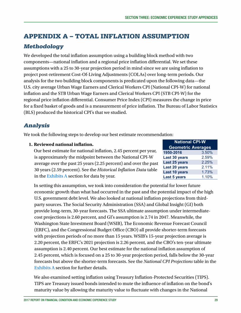
1. Reviewed national inflation. Our best estimate for national inflation, 2.45 percent per year,
is approximately the midpoint between the National CPI-W average over the past 25 years (2.25 percent) and over the past 30 years (2.59 percent). See the Historical Inflation Data table in the Exhibits A section for data by year.
In setting this assumption, we took into consideration the potential for lower future economic growth than what had occurred in the past and the potential impact of the high U.S. government debt level. We also looked at national inflation projections from third-party sources. The Social Security Administration (SSA) and Global Insight (GI) both provide long-term, 30-year forecasts. The SSA ultimate assumption under intermediate-cost projections is 2.60 percent, and GI’s assumption is 2.74 in 2047. Meanwhile, the Washington State Investment Board (WSIB), The Economic Revenue Forecast Council (ERFC), and the Congressional Budget Office (CBO) all provide shorter-term forecasts with projection periods of no more than 15 years. WSIB’s 15-year projection average is 2.20 percent, the ERFC’s 2021 projection is 2.26 percent, and the CBO’s ten-year ultimate assumption is 2.40 percent. Our best estimate for the national inflation assumption of 2.45 percent, which is focused on a 25 to 30-year projection period, falls below the 30-year forecasts but above the shorter-term forecasts. See the National CPI Projections table in the Exhibits A section for further details.
We also examined setting inflation using Treasury Inflation-Protected Securities (TIPS). TIPS are Treasury issued bonds intended to mute the influence of inflation on the bond’s maturity value by allowing the maturity value to fluctuate with changes in the National
1950-2016 3.50%Last 30 years 2.59%Last 25 years 2.25%Last 20 years 2.11%Last 10 years 1.73%Last 5 years 1.10%
National CPI-W Geometric Averages
30 2017 REPORT ON FINANCIAL CONDITION AND ECONOMIC EXPERIENCE STUDY
SECTION THREE: ECONOMIC EXPERIENCE STUDY APPENDICES
CPI. As such, TIPS can be used to approximate annual national inflation by subtracting off the TIPS yield from the yield of a non-inflation adjusted Treasury security with a similar maturity. However, we did not feel confident using TIPS to project inflation due to questions surrounding its liquidity and accuracy. For example, as WSIB notes in their 2017 Capital Market Assumptions (CMAs), because the size of the TIPS market is much smaller than that of nominal Treasury bonds, the yield of TIPS can become distorted due to an implicit “illiquidity premium” which has nothing to do with inflation.
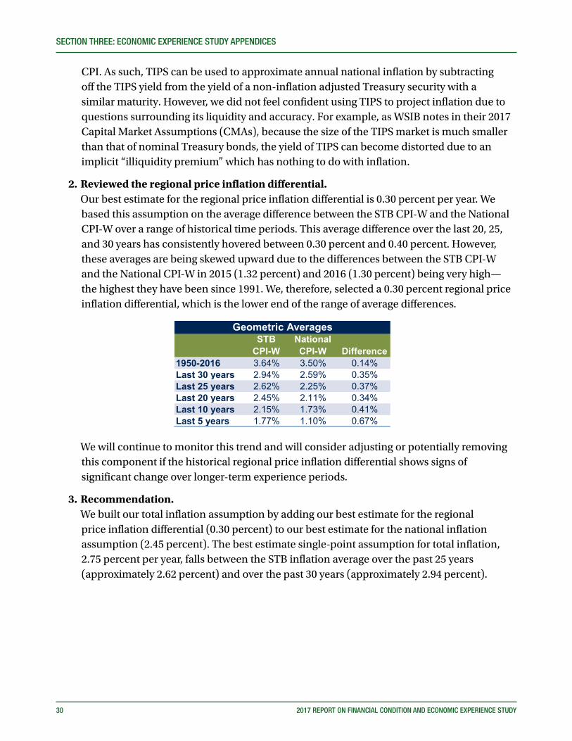
2. Reviewed the regional price inflation differential. Our best estimate for the regional price inflation differential is 0.30 percent per year. We
based this assumption on the average difference between the STB CPI-W and the National CPI-W over a range of historical time periods. This average difference over the last 20, 25, and 30 years has consistently hovered between 0.30 percent and 0.40 percent. However, these averages are being skewed upward due to the differences between the STB CPI-W and the National CPI-W in 2015 (1.32 percent) and 2016 (1.30 percent) being very high—the highest they have been since 1991. We, therefore, selected a 0.30 percent regional price inflation differential, which is the lower end of the range of average differences.
STB CPI-W
National CPI-W Difference
1950-2016 3.64% 3.50% 0.14%Last 30 years 2.94% 2.59% 0.35%Last 25 years 2.62% 2.25% 0.37%Last 20 years 2.45% 2.11% 0.34%Last 10 years 2.15% 1.73% 0.41%Last 5 years 1.77% 1.10% 0.67%
Geometric Averages
We will continue to monitor this trend and will consider adjusting or potentially removing this component if the historical regional price inflation differential shows signs of significant change over longer-term experience periods.
3. Recommendation. We built our total inflation assumption by adding our best estimate for the regional
price inflation differential (0.30 percent) to our best estimate for the national inflation assumption (2.45 percent). The best estimate single-point assumption for total inflation, 2.75 percent per year, falls between the STB inflation average over the past 25 years (approximately 2.62 percent) and over the past 30 years (approximately 2.94 percent).
SECTION THREE: ECONOMIC EXPERIENCE STUDY APPENDICES
2017 REPORT ON FINANCIAL CONDITION AND ECONOMIC EXPERIENCE STUDY 31
-1.0%
0.0%
1.0%
2.0%
3.0%
4.0%
5.0%
6.0%
7.0%
8.0%
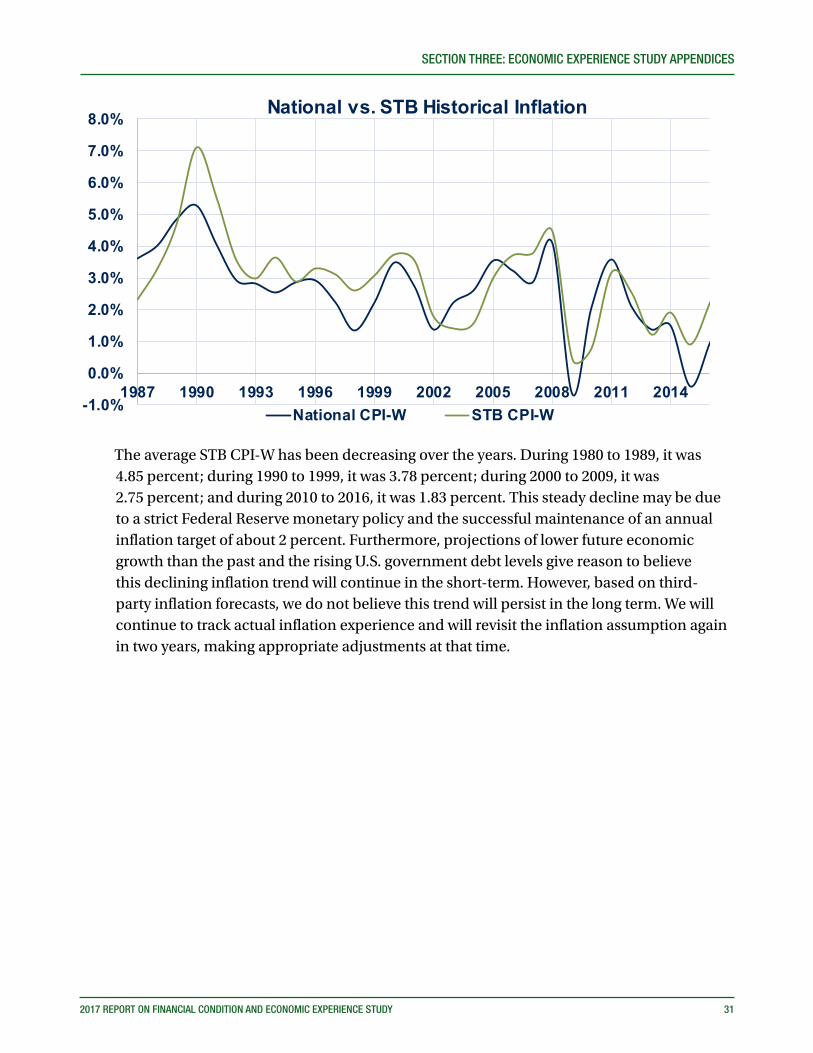
1987 1990 1993 1996 1999 2002 2005 2008 2011 2014
National vs. STB Historical Inflation
National CPI-W STB CPI-W
The average STB CPI-W has been decreasing over the years. During 1980 to 1989, it was 4.85 percent; during 1990 to 1999, it was 3.78 percent; during 2000 to 2009, it was 2.75 percent; and during 2010 to 2016, it was 1.83 percent. This steady decline may be due to a strict Federal Reserve monetary policy and the successful maintenance of an annual inflation target of about 2 percent. Furthermore, projections of lower future economic growth than the past and the rising U.S. government debt levels give reason to believe this declining inflation trend will continue in the short-term. However, based on third-party inflation forecasts, we do not believe this trend will persist in the long term. We will continue to track actual inflation experience and will revisit the inflation assumption again in two years, making appropriate adjustments at that time.

32 2017 REPORT ON FINANCIAL CONDITION AND ECONOMIC EXPERIENCE STUDY
SECTION THREE: ECONOMIC EXPERIENCE STUDY APPENDICES
Exhibits A
1987 318.6 335.0 2.35% 3.59% 2002 545.9 523.9 1.81% 1.37% 1988 329.1 348.4 3.30% 4.00% 2003 553.6 535.6 1.41% 2.23% 1989 344.5 365.2 4.68% 4.82% 2004 562.3 549.5 1.57% 2.60% 1990 369.0 384.4 7.11% 5.26% 2005 579.3 568.9 3.02% 3.53% 1991 389.4 399.9 5.53% 4.03% 2006 600.9 587.2 3.73% 3.22% 1992 403.2 411.5 3.54% 2.90% 2007 623.7 604.0 3.79% 2.86% 1993 415.2 423.1 2.98% 2.82% 2008 651.6 628.7 4.48% 4.09% 1994 430.4 433.8 3.66% 2.53% 2009 654.5 624.4 0.44% (0.67%)1995 442.9 446.1 2.90% 2.84% 2010 659.6 637.3 0.78% 2.07% 1996 457.5 459.1 3.30% 2.91% 2011 680.5 660.0 3.17% 3.56% 1997 471.7 469.3 3.10% 2.22% 2012 697.8 673.9 2.54% 2.10% 1998 484.1 475.6 2.63% 1.34% 2013 706.3 683.1 1.22% 1.37% 1999 499.1 486.2 3.10% 2.23% 2014 719.9 693.4 1.93% 1.50% 2000 517.8 503.1 3.75% 3.48% 2015 726.5 690.5 0.91% (0.41%)2001 536.2 516.8 3.55% 2.72% 2016 743.1 697.2 2.28% 0.98%
YearSTB
CPI-WNational CPI-W
Historical Inflation Data
Data source: Department of Labor, Bureau of Labor Statistics (BLS).
Year
Annual % ChangeSTB
CPI-WNational CPI-W
STB CPI-W
National CPI-W
Annual % ChangeSTB
CPI-WNational CPI-W
CBO ERFC GI SSA Int GI SSA Int2017 2.40% 2.47% 2.38% 2.76% 2033 2.67% 2.60%2018 2.30% 1.96% 1.92% 2.65% 2034 2.68% 2.60%2019 2.30% 1.99% 2.36% 2.60% 2035 2.66% 2.60%2020 2.40% 2.22% 2.73% 2.60% 2036 2.67% 2.60%2021 2.40% 2.26% 2.64% 2.60% 2037 2.67% 2.60%2022 2.40% 2.67% 2.60% 2038 2.69% 2.60%2023 2.40% 2.70% 2.60% 2039 2.70% 2.60%2024 2.40% 2.62% 2.60% 2040 2.70% 2.60%2025 2.40% 2.58% 2.60% 2041 2.72% 2.60%2026 2.40% 2.55% 2.60% 2042 2.73% 2.60%2027 2.40% 2.59% 2.60% 2043 2.74% 2.60%2028 2.60% 2.60% 2044 2.74% 2.60%2029 2.63% 2.60% 2045 2.74% 2.60%2030 2.64% 2.60% 2046 2.74% 2.60%2031 2.67% 2.60% 2047 2.74% 2.60%2032 2.67% 2.60%
National CPI Projections
The National SSA intermediate forecast is produced using a different basket of goods from the CBO, ERFC, and GI national projections. The SSA uses Urban Wage Earners and Clerical Workers while the other forecasts use All Urban Consumers. However, we do not believe an adjustment is required given the minor differences in the averages over the last 25 years.
SECTION THREE: ECONOMIC EXPERIENCE STUDY APPENDICES
2017 REPORT ON FINANCIAL CONDITION AND ECONOMIC EXPERIENCE STUDY 33
APPENDIX B – GENERAL SALARY GROWTH ASSUMPTION
MethodologyWe developed the general salary growth assumption using a building block method with two components—total inflation and real wage growth (which in previous studies, we had referred to as “productivity”). The Actuarial Standard of Practice 27 defines inflation as “price changes over the whole of the economy,” while real wage growth (or productivity) is defined as “the rates of change in a group’s compensation attributable to the change in real value of goods or services per unit of work.” We set these assumptions upon a 25- to 30-year horizon since we are ultimately using general salary growth to project wages over a member’s working lifetime in order to determine future retirement benefits and contribution rates.
AnalysisWe took the following steps to develop our best estimate recommendation:
1. Reviewed total inflation. We studied total inflation in depth and developed a best estimate of 2.75 percent for this
assumption, which we will be relying upon here. See the Total Inflation section of this report for information regarding the development of this assumption. With total inflation set, we next looked at real wage growth.
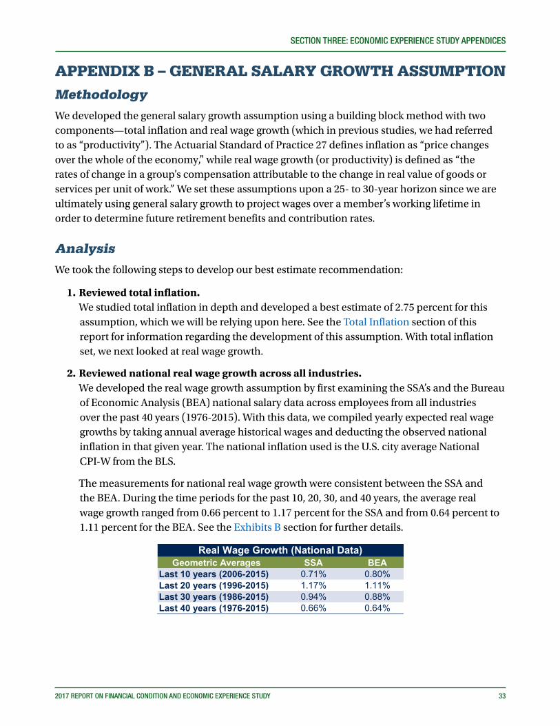
2. Reviewed national real wage growth across all industries. We developed the real wage growth assumption by first examining the SSA’s and the Bureau
of Economic Analysis (BEA) national salary data across employees from all industries over the past 40 years (1976-2015). With this data, we compiled yearly expected real wage growths by taking annual average historical wages and deducting the observed national inflation in that given year. The national inflation used is the U.S. city average National CPI-W from the BLS.
The measurements for national real wage growth were consistent between the SSA and the BEA. During the time periods for the past 10, 20, 30, and 40 years, the average real wage growth ranged from 0.66 percent to 1.17 percent for the SSA and from 0.64 percent to 1.11 percent for the BEA. See the Exhibits B section for further details.
Geometric Averages SSA BEALast 10 years (2006-2015) 0.71% 0.80%Last 20 years (1996-2015) 1.17% 1.11%Last 30 years (1986-2015) 0.94% 0.88%Last 40 years (1976-2015) 0.66% 0.64%
Real Wage Growth (National Data)
34 2017 REPORT ON FINANCIAL CONDITION AND ECONOMIC EXPERIENCE STUDY
SECTION THREE: ECONOMIC EXPERIENCE STUDY APPENDICES
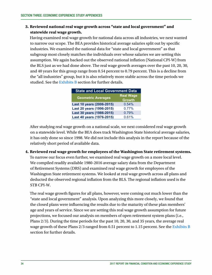
3. Reviewed national real wage growth across “state and local government” and statewide real wage growth.
Having examined real wage growth for national data across all industries, we next wanted to narrow our scope. The BEA provides historical average salaries split out by specific industries. We examined the national data for “state and local government” as that subgroup most closely matches the individuals over whose salaries we are setting this assumption. We again backed out the observed national inflation (National CPI-W) from the BLS just as we had done above. The real wage growth averages over the past 10, 20, 30, and 40 years for this group range from 0.54 percent to 0.79 percent. This is a decline from the “all industries” group, but it is also relatively more stable across the time periods we studied. See the Exhibits B section for further details.
Geometric Averages Real Wage Growth
Last 10 years (2006-2015) 0.54%Last 20 years (1996-2015) 0.77%Last 30 years (1986-2015) 0.79%Last 40 years (1976-2015) 0.61%
State and Local Government Data
After studying real wage growth on a national scale, we next considered real wage growth on a statewide level. While the BEA does track Washington State historical average salaries, it has only done so since 1998. We did not include this analysis in the report because of the relatively short period of available data.
4. Reviewed real wage growth for employees of the Washington State retirement systems. To narrow our focus even further, we examined real wage growth on a more local level.
We compiled readily available 1980-2016 average salary data from the Department of Retirement Systems (DRS) and examined real wage growth for employees of the Washington State retirement systems. We looked at real wage growth across all plans and deducted the observed regional inflation from the BLS. The regional inflation used is the STB CPI-W.
The real wage growth figures for all plans, however, were coming out much lower than the “state and local government” analysis. Upon analyzing this more closely, we found that the closed plans were influencing the results due to the maturity of these plan members’ age and years of service. Since we are setting this real wage growth assumption for future projections, we focused our analysis on members of open retirement system plans (i.e., Plans 2/3). During the time periods for the past 10, 20, 30, and 35 years, the average real wage growth of these Plans 2/3 ranged from 0.51 percent to 1.15 percent. See the Exhibits B section for further details.

SECTION THREE: ECONOMIC EXPERIENCE STUDY APPENDICES
2017 REPORT ON FINANCIAL CONDITION AND ECONOMIC EXPERIENCE STUDY 35
Geometric Averages Real Wage Growth
Last 10 years (2006-2015) 0.51%Last 20 years (1996-2015) 0.62%Last 30 years (1986-2015) 0.73%Last 35 years (1981-2015) 1.15%
Plans 2/3 Retirement System Data
5. Reviewed real wage growth forecasts. To help inform our decision on setting real wage growth, we reviewed projections of real
wage growth from the SSA and the CBO. As of 2016, the SSA has a 75-year projection of 1.2 percent for the total economy, and the CBO has a ten-year projection of 1.2 percent for the “non-farm business sector”. While both institutions set their real wage growth forecasts at a higher point-estimate than the historical 30-year geometric averages displayed above, neither institution has a significantly different forecast that it had in years prior.
The SSA’s 75-year projection of 1.2 percent is the same as their projection from four years earlier in their 2012 Trustees Report, and the CBO’s non-farm business sector ten-year projection of 1.2 percent is a slight decline from the 2002 to 2015 real wage growth experience for the nonfarm business sector of 1.3 percent. Our recommendation for real wage growth two years ago was 0.75 percent.
6. Expectations for the future. The last item we considered when studying real wage growth was our expectations for the
future. Moving forward, we do not expect future productivity to be as great as historical productivity. Some of the reasons for this expectation are as follows:
The climbing debt in the U.S. will lead to continued federal borrowing, which negatively affects the economy and productivity.1
The workforce population is aging which means a lower proportion of younger workers, who typically infuse new ideas, technologies, and improvements into the workplace.2
The rapid pace of informational and technological improvements over the past few decades has shown signs of diminishing.3
7. Recommendation. In developing our best estimate recommendation for real wage growth, we focused
most closely on the 30-year geometric averages. This gave us, what is in our professional judgment, a credible sample size, excluded the large negative impacts of the major recession of the late 1970’s and early 1980’s, and mirrored the 25- to 30-year horizon we are targeting in setting this assumption. These 30-year averages were as follows:
0.94 percent for the national data from the SSA.
1 CBO’s “Budget and Economic Outlook: 2017 to 2027.” 2 The Organisation for Economic Co-Operation and Development’s “Economic Surveys: United States 2016.” 3 Fernald, John G. 2015. “Productivity and Potential Output before, during, and after the Great Recession.” In NBER Macroeconomics Annual 2014,
Volume 29, edited by Jonathan A. Parker and Michael Woodford. Cambridge, MA: National Bureau of Economic Research, 1–51

36 2017 REPORT ON FINANCIAL CONDITION AND ECONOMIC EXPERIENCE STUDY
SECTION THREE: ECONOMIC EXPERIENCE STUDY APPENDICES
0.88 percent for the national data from the BEA.
0.79 percent for the “state and local government” national data from the BEA.
0.73 percent for the Plans 2/3 Washington State retirement system data from DRS.
Considering these historical averages together with third-party forecasts and our expectations for the future, we are maintaining the previous assumption for real wage growth of 0.75 percent.
Thus, in setting our recommendation for general salary growth, we combine our best estimate for total inflation (2.75 percent) with our best estimate for real wage growth (0.75 percent) and arrive at a recommended general salary growth assumption of 3.50 percent. This represents a 25 basis point reduction in the current assumption consistent with the recommended reduction in assumed inflation.
Exhibits B
Wage Growth Inflation1 Real Wage Growth
Last 10 years (2006-2015) 2.67% 1.96% 0.71%Last 20 years (1996-2015) 3.39% 2.21% 1.17%Last 30 years (1986-2015) 3.56% 2.61% 0.94%Last 40 years (1976-2015) 4.39% 3.70% 0.66%
Last 10 years (2006-2015) 2.77% 1.96% 0.80%Last 20 years (1996-2015) 3.33% 2.21% 1.11%Last 30 years (1986-2015) 3.50% 2.61% 0.88%Last 40 years (1976-2015) 4.37% 3.70% 0.64%
Last 10 years (2006-2015) 2.52% 1.96% 0.54%Last 20 years (1996-2015) 2.99% 2.21% 0.77%Last 30 years (1986-2015) 3.41% 2.61% 0.79%Last 40 years (1976-2015) 4.34% 3.70% 0.61%
Last 10 years (2006-2015) 2.81% 2.29% 0.51%Last 20 years (1996-2015) 3.14% 2.51% 0.62%Last 30 years (1986-2015) 3.63% 2.89% 0.73%Last 40 years (1976-2015) 4.27% 3.11% 1.15%
4 Annual wage data from the BEA. Wages based on salaries for full-time equivalent state and local government employees.
Historical Geometric AveragesTime Period
National Data (SSA - All Industries)2
National Data (BEA - All Industries)3
National Data (BEA - State and Local Government)4
Retirement System Data (DRS - Plans 2/3)5
Note: A real wage growth is calculated for each year as wage growth less inflation. It is the geometric average of these values that is displayed in the "real wage growth" column, which does not always necessarily align with the geometric average of wage growth less the geometric average of inflation.1 Inflation for "Retirement System Data (DRS - Plans 2/3)" uses the Seattle-Tacoma-Bremerton CPI-W data from the BLS. All other inflations use the National CPI-W data.2 Annual wage data from the SSA. Wages based on compensation (wages, tips, etc) subject to Federal income taxes.3 Annual wage data from the BEA. Wages based on salaries for full-time equivalent employees across all industries.
5 Annual wage data from DRS. Wages based on salaries for full-time equivalent employees across the retirement systems Plans 2/3.

SECTION THREE: ECONOMIC EXPERIENCE STUDY APPENDICES
2017 REPORT ON FINANCIAL CONDITION AND ECONOMIC EXPERIENCE STUDY 37
APPENDIX C – INVESTMENT RATE OF RETURN ASSUMPTION
MethodologyThe recommended rate of investment return assumption represents the anticipated returns on the Commingled Trust Fund’s (CTF) current and future assets, net of expenses. We apply this assumption as a single rate to all plans invested in the CTF. We based the rate on the average future measurement period – referred to as duration – for all plans combined. However, not all plans have the same duration. Plan 1 liabilities have a shorter duration than the liabilities of Plans 2/3. This occurs because the Plans 1 for all systems, except the Washington State Patrol Retirement System (WSPRS), have been closed to new entrants since 1977 (WSPRS plan 1 closed in 2002), while the Plans 2/3 are still open to new entrants. This means that all Plan 1 benefits will be paid well before the last Plans 2/3 benefits are paid – hence the shorter future measurement period or duration for the Plans 1.
The rate of investment return assumption is coordinated with WSIB’s current asset allocation policy, or targets, for the CTF. Future changes to the CTF asset allocation policy or CMAs may require a new recommendation for the rate of investment return assumption.
We used the “building block” method to develop this assumption. Using this method, the actuary determines the individual components for each economic assumption. Then the actuary may combine estimates for each applicable component to arrive at a best estimate for the given economic assumptions.
In setting this assumption, we reviewed past investment returns and WSIB’s expectation for future investment returns. For future returns, we reviewed the simulated market returns from the current target asset allocation and CMAs provided by WSIB. We also reviewed WSIB’s inflation assumption to ensure consistency of the return assumption with the entire set of economic assumptions for this study. Lastly, we considered the sensitivity of the simulated returns to different CMAs and asset allocations.
AnalysisWe took the following steps to develop our best estimate recommendation:
1. Reviewed historical investment returns. The following table summarizes the historical investment returns we observed over the
given time periods. See the Exhibits C section for historical returns by year.
We observed that the average investment return is very sensitive to the time period. For example, inclusion of the Great Recession returns lowers the ten-year average return significantly compared to averages for time periods greater
Past 5 Years 10.30%Past 10 Years 5.63%Past 15 Years 8.35%Past 20 Years 7.66%Past 30 Years 8.78%
Historical WSIB Annual Average Returns
Source: Washington State Investment Board. Returns restated for 1993 and beyond.

38 2017 REPORT ON FINANCIAL CONDITION AND ECONOMIC EXPERIENCE STUDY
SECTION THREE: ECONOMIC EXPERIENCE STUDY APPENDICES
than ten years. Similarly, the five-year average contains large returns as investment markets recovered from the Great Recession. Over the long-term, WSIB has produced returns in excess of the assumed rate of return for the period.
Relying on historical data in setting a forward-looking investment returns assumption requires us to assume that the economic conditions that produced past returns will continue in the future. However, the national and world economy continues to change.
The following list demonstrates how economic conditions have changed and the possible impacts on future returns:
Globalization and fewer emerging markets. Investors have historically targeted emerging markets for investment opportunities
with large growth potential. Globalization has sped up the development of many emerging markets and left fewer investment prospects.
Stock market returns will likely revert to historical averages. When the economy is experiencing high growth, stock market valuations as
measured by their Price to Earnings (P/E) Ratio tend to increase, meaning investors are willing to pay more for the same amount of earnings, all else held constant. Over the last 30 years, the Standard and Poor’s (S&P) 500 P/E Ratio has increased significantly. However, with lower expected growth going forward, the P/E Ratio for the S&P 500 may revert to lower historical levels. A decrease in the P/E Ratio will have a negative impact on prices, and therefore lower future stock market returns.
Technological disruptions. Advances in technology have led to shrinking margins on goods and fewer well-paying
labor jobs. For example, online retailers, such as Amazon, allow for easy comparison of goods. This effectively increases competition between retailers and shrinks profit margins for potential investors. Likewise, the manufacturing industry has moved away from a labor focus and toward automation. Manufacturing will require less workers in traditionally well-paid jobs, which causes deflation in the economy as a whole.
Low productivity growth. Productivity growth describes the increase in output for each unit of input, such as
a workers ability to produce more goods while working the same number of hours. Productivity growth has steadily increased over the 20th century but has slowed over the last decade. Sustained low productivity growth will lead to poorer economic growth compared to prior decades.
Increasing Government debt. The amount of U.S. government debt has risen to historic levels. The use of debt
(or “leverage”) generally improves returns. However, paying down or stabilizing a large debt requires cutting from other programs or raising taxes, both of which hurt

SECTION THREE: ECONOMIC EXPERIENCE STUDY APPENDICES
2017 REPORT ON FINANCIAL CONDITION AND ECONOMIC EXPERIENCE STUDY 39
prospective economic growth. In the event of another economic downturn, a large amount of debt limits the government’s ability to provide economic stimulus.
Population demographics shift. The general population is getting older as the Baby Boomers move toward
retirement. We expect the shift of a large percentage of the population leaving the work force and moving into retirement to lower economic growth.
Inflation could be lower in the future. With a low growth forecast and a low interest rate environment, inflation could be
lower than what we have historically witnessed. Our analysis and recommendation for inflation in this study also suggests lower future inflation. As investment returns are comprised of real returns plus inflation, lower inflation will have a negative impact on investment returns.
The list above is not exhaustive, but rather is meant to illustrate how conditions are different now compared to what has been true in the past and how those different conditions could produce lower future returns.
2. Reviewed Expectations for the Future - WSIB’s CMAs and simulated future investment returns.
WSIB assigns three pieces of information to each asset class they invest in to form the CMAs:
Expected annual return.
Standard deviation of the annual return.
Correlations between the annual returns of each asset class with every other asset class.
WSIB then uses the CMAs and their target asset allocation under an assumed distribution model to project (or simulate) future investment returns. The following table displays the expected annual return, standard deviation, and target asset allocation for this study and the prior study. Please see WSIB’s 2017 White Paper for asset class correlations and modeling applications.

40 2017 REPORT ON FINANCIAL CONDITION AND ECONOMIC EXPERIENCE STUDY
SECTION THREE: ECONOMIC EXPERIENCE STUDY APPENDICES
2017 Asset Class 2017 2015 Difference 2017 2015 DifferenceGlobal Equity 8.5% 8.8% (0.3%) 18.00% 18.85% (0.85%)Tangible Assets 7.1% 6.6% 0.5% 13.00% 8.60% 4.40%Fixed Income 3.9% 3.9% 0.0% 5.50% 5.25% 0.25%Private Equity 11.5% 11.8% (0.3%) 25.00% 25.00% 0.00%Real Estate 8.0% 8.0% 0.0% 14.00% 15.70% (1.70%)Cash 2.3% 2.3% 0.0% 1.00% 2.00% (1.00%)
Total*No change in target asset allocation between 2017 and 2015 Economic Experience Studies.
100%
WSIB Portfolio Statistics & Capital Market AssumptionsTarget Allocation* Expected 1-Year Return Standard Deviation
37%5%
20%23%15%0%
Moving from the 2015 to the 2017 CMAs, we see a decrease in the one-year expected return and standard deviation (or volatility). Together, the lower expected return and volatility will create smaller but less dispersed projected returns. Please see the Exhibits C section for a comparison of the expected annual return, standard deviation, and target asset allocation for this study and the prior four experience studies.
WSIB provided our office with simulations under varying forecast periods. WSIB creates return simulations by randomizing annual returns using the CMA statistics and target asset allocation. They then calculate an average annual return for the simulation and repeat the process many times. WSIB provided us with the simulated annual investment returns at various percentiles for time horizons ranging from one year to 50 years.
The following table displays the annual return from 50-year simulations for the current and 2015 study. Please see the Exhibits C section for 50-year simulated annual investment returns for this study and the prior four experience studies.
Comparing the results for the 2015 and 2017 study, the 50-year median annual return decreased from 7.74 percent to 7.34 percent. We can interpret the median return as the return that splits half of all simulations above and half below that value. Put another way, using the assumptions from the simulations, there is a 50 percent chance returns will exceed the median return and a 50 percent chance they will fall below the median return.
The simulated future investment returns represent WSIB’s best estimate of future returns for the CTF, but require a number of simplifying assumptions. The simulated returns are calculated assuming the target asset allocation and CMAs will remain constant throughout the projection period. However, actual asset allocation may vary from the targets and actual market performance may vary from the CMAs. Future asset-allocation targets and CMAs may vary from the current values as well.
2017 2015 Difference75th percentile 8.57% 8.86% (0.29%)60th percentile 7.81% 8.18% (0.37%)55th percentile 7.58% 7.94% (0.36%)Median Return 7.34% 7.74% (0.40%)45th percentile 7.11% 7.54% (0.43%)40th percentile 6.87% 7.31% (0.44%)25th percentile 6.08% 6.56% (0.48%)*Source: Washington State Investment Board.
50-Year Simulated Future Investment Returns*

SECTION THREE: ECONOMIC EXPERIENCE STUDY APPENDICES
2017 REPORT ON FINANCIAL CONDITION AND ECONOMIC EXPERIENCE STUDY 41
It is important to note that WSIB sets and applies their CMAs over a 15-year period only. We apply the assumptions over a longer period, 30 to 50 years, for purposes of determining funding requirements consistent with current state funding policy. As noted in the Recommendation section, we apply adjustments using our professional judgment to arrive at assumptions consistent with a measurement period significantly longer than 15 years.
3. Reviewed sensitivity of the simulated returns to the CMAs. As with any assumption, we recognize that the CMAs may not match reality so we reviewed
how WSIB simulated returns change under a different set of CMAs. To do this, we observed the impact of adjusting the expected annual return of the largest target asset allocations.
We looked at increasing or decreasing the expected one-year return of global equities and private equities by one percent. We chose these two asset classes because they compromise sixty percent of the target total portfolio allocation and have the greatest amount of uncertainty around their return. The table below displays the simulated annual returns for the sensitivity analysis.
Base -1% +1% -1% +1%8.57% 8.34% 8.80% 8.20% 8.94%7.81% 7.58% 8.05% 7.44% 8.19%7.58% 7.34% 7.81% 7.20% 7.95%7.34% 7.11% 7.57% 6.97% 7.71%7.11% 6.88% 7.34% 6.74% 7.48%6.87% 6.64% 7.10% 6.50% 7.24%6.08% 5.85% 6.32% 5.71% 6.46%
50-Year Simulated Annual Investment Returns - Sensitivity AnalysisPrivate Equity -
Expected ReturnGlobal Equity -
Expected Return
75th percentile60th percentile55th percentileMedian Return45th percentile40th percentile25th percentile
If we assume that private equity or global equity will return one percent lower, on average, then the simulated return decreases at all percentiles. This means that in the case of a one percent decrease in the global equity average return, there is about a 50 percent likelihood, using the assumptions from the simulations, that CTF median annual returns over 50 years would fall below seven percent. On the other hand, for a one percent increase in the average return for private or global equities, we observe an increase in the simulated return for all percentiles. In the case of a one percent increase in the global equity average return, there is about a 50 percent likelihood, using the assumptions for the simulations, that CTF median annual returns over 50 years would fall below 7.71 percent.
4. Recommendation. After reviewing past investment performance and expectations for the future, we used our
professional judgement to make the following adjustments to WSIB’s simulated returns:
Increased simulated returns by 25 basis points (0.25 percent) – to reflect the difference between WSIB and our inflation assumptions. In the CMAs, WSIB assumes 15-year national inflation of 2.20 percent each year. In this study, we
42 2017 REPORT ON FINANCIAL CONDITION AND ECONOMIC EXPERIENCE STUDY
SECTION THREE: ECONOMIC EXPERIENCE STUDY APPENDICES
recommend a long-term national inflation assumption of 2.45 percent. We believe this adjustment is necessary to retain consistency between the entire set of economic assumptions.
Decreased simulated returns for Private Equity (PE) – to reflect assumptions consistent with a longer time horizon. We believe WSIB’s CMAs for PE are reasonable and appropriate for a 15-year time horizon. However, when we extend this assumption over 50 years, we implicitly assume the PE performance expected for the next 15 years will continue for 50 years. As this asset class continues to mature and evolve, we expect increased competition for PE investment opportunities and more efficient PE markets. These factors, in our judgment, would lead to lower long-term PE returns than observed in the past and expected over the next 15 years.
With these adjustments, and other considerations noted in this analysis, we arrive at a recommended long-term rate of return of 7.4 percent.
For context only, if you assume 1 percent lower annual PE returns than current WSIB CMAs, and add 25 basis points for differences in assumed inflation as noted above, the median 50-year annual return would equal 7.36 percent (7.11% + 0.25%). Additionally, given the inherent uncertainty with future returns, it may be appropriate to include some margin for “adverse deviation” when adopting a long-term return assumption. The 45th percentile of simulated annual returns over the next 50 years plus the 25 basis point adjustment for inflation equals 7.36 percent (this excludes any adjustment to assumed PE returns). Using the 45th percentile, instead of the 50th percentile (the median), implies a 55 percent chance of meeting or exceeding the given return instead of a 50 percent chance.
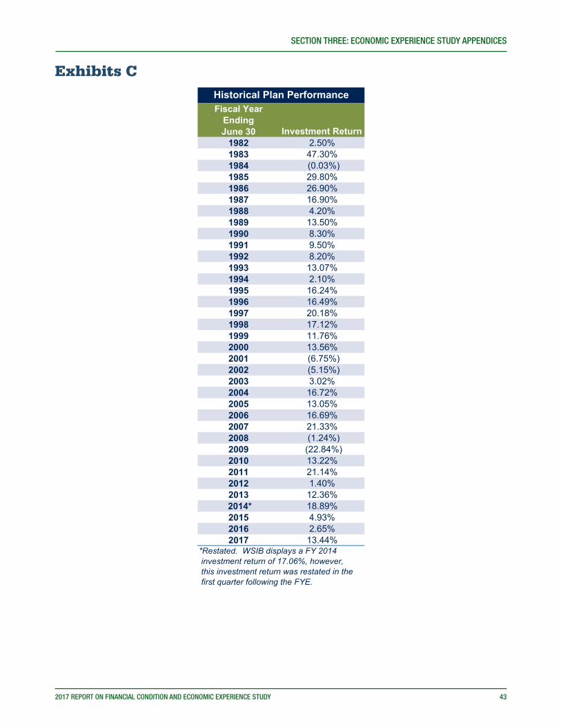
SECTION THREE: ECONOMIC EXPERIENCE STUDY APPENDICES
2017 REPORT ON FINANCIAL CONDITION AND ECONOMIC EXPERIENCE STUDY 43
Exhibits C
Fiscal YearEndingJune 30
1982 2.50%1983 47.30%1984 (0.03%)1985 29.80%1986 26.90%1987 16.90%1988 4.20%1989 13.50%1990 8.30%1991 9.50%1992 8.20%1993 13.07%1994 2.10%1995 16.24%1996 16.49%1997 20.18%1998 17.12%1999 11.76%2000 13.56%2001 (6.75%)2002 (5.15%)2003 3.02%2004 16.72%2005 13.05%2006 16.69%2007 21.33%2008 (1.24%)2009 (22.84%)2010 13.22%2011 21.14%2012 1.40%2013 12.36%
2014* 18.89%2015 4.93%2016 2.65%2017 13.44%
Historical Plan Performance
Investment Return
*Restated. WSIB displays a FY 2014 investment return of 17.06%, however, this investment return was restated in the first quarter following the FYE.
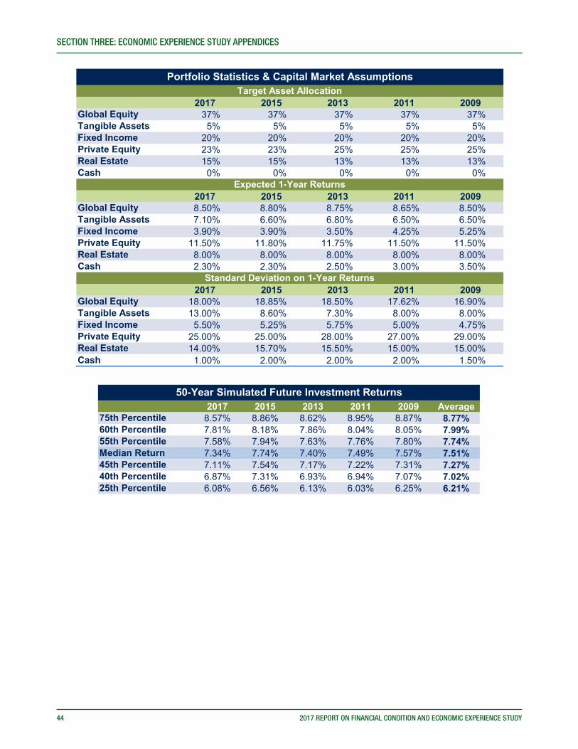
44 2017 REPORT ON FINANCIAL CONDITION AND ECONOMIC EXPERIENCE STUDY
SECTION THREE: ECONOMIC EXPERIENCE STUDY APPENDICES
2017 2015 2013 2011 200937% 37% 37% 37% 37%5% 5% 5% 5% 5%
20% 20% 20% 20% 20%23% 23% 25% 25% 25%15% 15% 13% 13% 13%0% 0% 0% 0% 0%
2017 2015 2013 2011 20098.50% 8.80% 8.75% 8.65% 8.50%7.10% 6.60% 6.80% 6.50% 6.50%3.90% 3.90% 3.50% 4.25% 5.25%
11.50% 11.80% 11.75% 11.50% 11.50%8.00% 8.00% 8.00% 8.00% 8.00%2.30% 2.30% 2.50% 3.00% 3.50%
2017 2015 2013 2011 200918.00% 18.85% 18.50% 17.62% 16.90%13.00% 8.60% 7.30% 8.00% 8.00%5.50% 5.25% 5.75% 5.00% 4.75%
25.00% 25.00% 28.00% 27.00% 29.00%14.00% 15.70% 15.50% 15.00% 15.00%
1.00% 2.00% 2.00% 2.00% 1.50%
Global Equity
Portfolio Statistics & Capital Market AssumptionsTarget Asset Allocation
Global EquityTangible AssetsFixed IncomePrivate EquityReal EstateCash
Expected 1-Year Returns
Cash
Tangible AssetsFixed IncomePrivate EquityReal EstateCash
Standard Deviation on 1-Year Returns
Global EquityTangible AssetsFixed IncomePrivate EquityReal Estate
2017 2015 2013 2011 2009 Average8.57% 8.86% 8.62% 8.95% 8.87% 8.77%7.81% 8.18% 7.86% 8.04% 8.05% 7.99%7.58% 7.94% 7.63% 7.76% 7.80% 7.74%7.34% 7.74% 7.40% 7.49% 7.57% 7.51%7.11% 7.54% 7.17% 7.22% 7.31% 7.27%6.87% 7.31% 6.93% 6.94% 7.07% 7.02%6.08% 6.56% 6.13% 6.03% 6.25% 6.21%
40th Percentile25th Percentile
50-Year Simulated Future Investment Returns
75th Percentile60th Percentile55th PercentileMedian Return45th Percentile
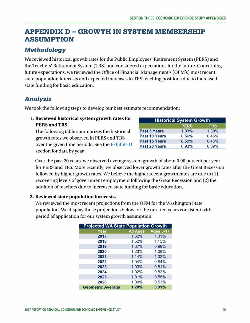
SECTION THREE: ECONOMIC EXPERIENCE STUDY APPENDICES
2017 REPORT ON FINANCIAL CONDITION AND ECONOMIC EXPERIENCE STUDY 45
APPENDIX D – GROWTH IN SYSTEM MEMBERSHIP ASSUMPTION
MethodologyWe reviewed historical growth rates for the Public Employees’ Retirement System (PERS) and the Teachers’ Retirement System (TRS) and considered expectations for the future. Concerning future expectations, we reviewed the Office of Financial Management’s (OFM’s) most recent state population forecasts and expected increases in TRS teaching positions due to increased state funding for basic education.
AnalysisWe took the following steps to develop our best estimate recommendation:
1. Reviewed historical system growth rates for PERS and TRS.
The following table summarizes the historical growth rates we observed in PERS and TRS over the given time periods. See the Exhibits D section for data by year.
Over the past 20 years, we observed average system growth of about 0.90 percent per year for PERS and TRS. More recently, we observed lower growth rates after the Great Recession followed by higher growth rates. We believe the higher recent growth rates are due to (1) recovering levels of government employment following the Great Recession and (2) the addition of teachers due to increased state funding for basic education.
2. Reviewed state population forecasts. We reviewed the most recent projections from the OFM for the Washington State
population. We display those projections below for the next ten years consistent with period of application for our system growth assumption.
Year All Ages Ages 5-172017 1.62% 1.31%2018 1.52% 1.15%2019 1.37% 0.98%2020 1.23% 1.08%2021 1.14% 1.02%2022 1.04% 0.84%2023 1.03% 0.81%2024 1.02% 0.82%2025 1.01% 0.58%2026 1.00% 0.53%
Geometric Average 1.20% 0.91%
Projected WA State Population Growth
PERS TRSPast 5 Years 1.03% 1.38%Past 10 Years 0.56% 0.46%Past 15 Years 0.59% 0.46%Past 20 Years 0.93% 0.89%
Historical System Growth

46 2017 REPORT ON FINANCIAL CONDITION AND ECONOMIC EXPERIENCE STUDY
SECTION THREE: ECONOMIC EXPERIENCE STUDY APPENDICES
As indicated in the table, OFM expects the overall state population to grow just under 1.20 percent each year on average for the next ten years and the school-age population to grow just over 0.91 percent each year on average over the next ten years.
3. Expectations for the future. If the retirement systems grew at the same rate as the state population, we would expect
annual growth rates of about 1.20 percent and 0.90 percent for PERS and TRS respectively for the next ten years. This compares to an observed annual growth rate of 0.90 percent for both PERS and TRS over the last 20 years.
Over the last 20 years, PERS has grown at a lower annual rate than the state population and TRS has grown at a higher annual rate than the school-age population. See the Exhibits D section for further details.
In the long term, we expect both PERS and TRS to grow at a lower rate than the state population. Over the next two years, we expect PERS to continue to grow at rates higher than currently expected due to recovering levels of government employment following the Great Recession. For TRS, we expect above average growth due to new teaching positions from increased state funding for basic education.
4. Recommendation. When we apply our expectations for the future to OFM’s state population forecasts,
we arrive at our preliminary projected retirement system growth rates. We display the preliminary growth rates in the table below.
Year PERS TRS2017 1.03% 1.31%2018 1.03% 5.08%*2019 1.23% 0.88%2020 1.10% 0.97%2021 1.03% 0.92%2022 0.93% 0.76%2023 0.93% 0.73%2024 0.92% 0.73%2025 0.91% 0.53%2026 0.90% 0.48%
Geometric Average 1.00% 1.23%
Preliminary Annual Growth Rates
*Increased growth rate for OFM's expected number of new teachers from class size reduction funding in 2017-19 budget.
For PERS, we assume the system will grow for the next two years at the average observed growth rate for the past five years. After the next two years, we assume PERS will grow at 90 percent of the total state population growth rate. This produces an average annual growth rate of 1.00 percent for PERS over the next ten years. Given the uncertainty involved in setting this assumption, we believe the current assumption of 0.95 percent remains reasonable and we recommend no change to this assumption.

SECTION THREE: ECONOMIC EXPERIENCE STUDY APPENDICES
2017 REPORT ON FINANCIAL CONDITION AND ECONOMIC EXPERIENCE STUDY 47
For TRS, we assume the system will grow for the next two years at the same rate as the school-age population with one adjustment in FY 2018 (as noted in the following paragraph). After the next two years, we assume TRS will grow at 90 percent of the school-age population growth rate. This produces an average annual growth rate of 1.23 percent for TRS over the next ten years. Given the uncertainty involved in setting this assumption, and the uncertainty of the number of new teaching positions the state will add in the future due to increased state funding for basic education, we believe the current assumption of 1.25 percent remains reasonable and we recommend no change to this assumption.
Our adjustment to TRS growth rates in FY 2018 reflects OFM’s estimate of new teaching positions funded in the 2017-19 budget above typical system growth. We assumed 50 percent of positions funded in the budget would result in new hires due to a number of limiting factors. These include but are not limited to the following: (1) some new teachers have already been hired using local funds and this additional funding will shift funding from local to state sources instead of result in more teachers, (2) the supply of new teachers may not meet the demand, and (3) the current school infrastructure only supports a limited number of new classrooms. This led to an increase of about 2,800 new teachers in FY 2018 on top of additional teaching positions from school age population growth.
We created a single assumption for each system by averaging the ten years of projected system growth. The static system growth assumption applies to each year of our valuation rather than varying by year.

48 2017 REPORT ON FINANCIAL CONDITION AND ECONOMIC EXPERIENCE STUDY
SECTION THREE: ECONOMIC EXPERIENCE STUDY APPENDICES
Exhibits D
# of
Act
ive
Mem
bers
Annu
al
Gro
wth
# of
Pe
ople
Annu
al
Gro
wth
# of
Act
ive
Mem
bers
Annu
al
Gro
wth
# of
Pe
ople
Annu
al
Gro
wth
1995
178,
833
0.78
%5,
396,
569
1.98
%59
,103
2.38
%1,
009,
134
2.34
%19
9618
2,60
32.
11%
5,48
3,10
31.
60%
59,4
250.
54%
1,02
8,78
51.
95%
1997
186,
440
2.10
%5,
579,
140
1.75
%60
,815
2.34
%1,
050,
205
2.08
%19
9819
1,85
02.
90%
5,68
5,45
91.
91%
61,8
281.
67%
1,07
3,56
42.
22%
1999
196,
382
2.36
%5,
792,
214
1.88
%62
,684
1.38
%1,
097,
002
2.18
%20
0019
9,98
61.
84%
5,89
4,14
31.
76%
63,8
581.
87%
1,11
9,53
32.
05%
2001
201,
283
0.65
%5,
970,
452
1.29
%66
,220
3.70
%1,
120,
486
0.09
%20
0220
3,97
61.
34%
6,05
9,69
81.
49%
66,0
63(0
.24%
)1,
123,
863
0.30
%20
0320
3,76
4(0
.10%
)6,
126,
917
1.11
%66
,075
0.02
%1,
123,
183
(0.0
6%)
2004
206,
110
1.15
%6,
208,
532
1.33
%66
,634
0.85
%1,
125,
174
0.18
%20
0520
5,92
8(0
.09%
)6,
298,
797
1.45
%67
,270
0.95
%1,
128,
718
0.31
%20
0620
7,91
80.
97%
6,42
0,21
91.
93%
67,7
360.
69%
1,13
7,75
60.
80%
2007
211,
602
1.77
%6,
525,
121
1.63
%64
,939
(4.1
3%)
1,14
3,75
00.
53%
2008
217,
423
2.75
%6,
608,
234
1.27
%66
,524
2.44
%1,
145,
885
0.19
%20
0921
6,04
9(0
.63%
)6,
672,
263
0.97
%67
,388
1.30
%1,
144,
749
(0.1
0%)
2010
213,
075
(1.3
8%)
6,72
4,54
00.
78%
66,3
25(1
.58%
)1,
141,
697
(0.2
7%)
2011
208,
936
(1.9
4%)
6,76
7,90
00.
64%
66,2
03(0
.18%
)1,
135,
411
(0.5
5%)
2012
206,
398
(1.2
1%)
6,81
7,77
00.
74%
65,3
57(1
.28%
)1,
135,
901
0.04
%20
1320
7,51
40.
54%
6,88
2,40
00.
95%
65,9
350.
88%
1,14
1,79
70.
52%
2014
211,
063
1.71
%6,
968,
170
1.25
%67
,293
2.06
%1,
151,
551
0.85
%20
1521
4,30
41.
54%
7,06
1,41
01.
34%
68,8
202.
27%
1,16
2,41
70.
94%
2016
219,
891
2.61
%7,
183,
700
1.73
%70
,915
3.04
%1,
178,
014
1.34
%G
eom
etric
Ave
rage
s:Pa
st 5
Yea
rs1.
03%
1.20
%1.
38%
0.74
%Pa
st 1
0 Ye
ars
0.56
%1.
13%
0.46
%0.
35%
Past
15
Year
s0.
59%
1.24
%0.
46%
0.33
%Pa
st 2
0 Ye
ars
0.93
%1.
36%
0.89
%0.
68%
*Sou
rce:
Dep
artm
ent o
f Ret
irem
ent S
yste
ms
and
Offi
ce o
f Fin
anci
al M
anag
emen
t. A
dditi
onal
com
puta
tions
hav
e be
en p
erfo
rmed
to s
umm
ariz
e da
ta.
His
toric
al S
yste
m G
row
th*
WA
Popu
latio
nYe
arPE
RS
WA
Popu
latio
nTR
SAg
es 5
-17


2017 Report on Financial Condition and Economic Experience StudyPREPARED FOR THE PENSION FUNDING COUNCIL • AUGUST 2017
Office of the State Actuary“Supporting financial security for generations.”