2017, Attiya Darensburg - TDL
118
Global mapping of the 410 km upper mantle boundary using PP precursor waves by Attiya Darensburg, M.S. A Thesis In Geoscience Submitted to the Graduate Faculty of Texas Tech University in Partial Fulfillment of the Requirements for the Degree of Master of Science Approved Dr. Harold Gurrola Chair of Committee Dr. Hal Karlsson Dr. George Asquith Mark Sheridan Dean of the Graduate School August, 2017
Transcript of 2017, Attiya Darensburg - TDL

Global mapping of the 410 km upper mantle boundary using PP precursor waves
by
Attiya Darensburg, M.S.
A Thesis
In
Geoscience
Submitted to the Graduate Faculty
of Texas Tech University in
Partial Fulfillment of
the Requirements for
the Degree of
Master of Science
Approved
Dr. Harold Gurrola
Chair of Committee
Dr. Hal Karlsson
Dr. George Asquith
Mark Sheridan
Dean of the Graduate School
August, 2017

© 2017, Attiya Darensburg

Texas Tech University, Attiya Darensburg, August 2017
ii
ACKNOWLEDGMENTS
I would like to extend my gratitude toward my advisor, Dr. Gurrola for his patience
and guidance throughout my academic endeavors at Texas Tech University. I would
also like to thank him especially for his immense guidance with MATLAB and
troubleshooting. I have enjoyed being his student a great deal and I have flourished
under his mentorship. I have also enjoyed the casual conversations about current
events with heaping doses of humorous commentary. I would also like to take the time
out to thank the other members of my committee, Dr. Asquith and Dr. Karlsson, for
graciously making themselves available to serve on my defense committee.
Last, but definitely not least, I would like to thank my mother, Barbara Darensburg,
for her support throughout my life and always being there for words of encouragement
and unconditional love. Through the sacrifices she made for me as a child and into
adulthood, I am able to be the woman and scholar that I am today and words really
cannot express how much she means to me. I would like to also thank friends and
family who have been a tremendous source of support throughout my life.

Texas Tech University, Attiya Darensburg, August 2017
iii
TABLE OF CONTENTS
ACKNOWLEDGMENTS……………………………….......................................... ii
ABSTRACT ………………………………………………………............................ v
LIST OF TABLES …………………………………………………………………. vi
LIST OF FIGURES ……………………………………………………………….. vii
I. INTRODUCTION ……………………………………………………………….. 1
II. GEOLOGICAL BACKGROUND …………………………………………….. 4
Pyrolite vs Piclogite Mantle ……………………………………........................... 4
Previous studies using seismic waveforms to image discontinuities
at 410, 520, and 660 km ………………………………………………………… 10
III. METHODS …………………………………………………….......................... 23
Data processing …………………………………………………………………. 23
Crustal tests ……………………………………………………………………... 30
IV. RESULTS ……………………………………………………………………… 37
PP precursor functions beneath Hawaii ………………………………………… 43
PP precursor functions beneath Alaska………………………….......................... 46
PP precursor functions beneath Eurasia…………………………………………. 49
PP precursor functions beneath northwestern Europe, Greenland,
and Iceland ……………………………………………………………………… 53
PP precursor functions beneath South America…………………......................... 57
V. DISCUSSION …………………………………………………………………... 61
Analysis of global variations in the 410 km discontinuity using
PP precursors …………………………………………………………………… 61
Hawaii ……………………………………………………………....................... 62
Alaska and the Aleutian Islands …...………………………..…........................... 65
Eurasia and N. India …………………………………………….......................... 68
Greenland and Iceland ……………………………………………...................... 73
VI. CONCLUSION ………………………………………………………………... 77
WORKS CITED …………………………………………………………………… 80

Texas Tech University, Attiya Darensburg, August 2017
iv
APPENDICES
A. USER MANUALS …………………………………………………………..... 87
B. QC GUIDE ……………………………………………………………………. 91

Texas Tech University, Attiya Darensburg, August 2017
v
ABSTRACT
Globally mapping the mineral phase discontinuities in the earth’s upper mantle
will enable us to develop detailed 1D models of the upper mantle discontinuity at 410
km depth using underside reflections from PP precursor waves. The 520 km
discontinuity has proven difficult to image with PP waves due to interference from
sidelobes from reflections off of the underside of discontinuity boundaries at 410 km
and 660 km depth. PP precursors cannot be used to map the 660 km discontinuity
either since the reflection from this boundary does not appear consistently. We have
stacked and binned 25 years-worth of seismic data collected between 1990 and 2015
from stations all over the globe available from the IRIS data management services
(DMC). Using the stacked PP functions, we will assess the behavior of the 410 km
discontinuity in regions where there are significant temperature anomalies based on
the mapped depth of the 410 and amplitude of the pulses reflected from this
discontinuity.

Texas Tech University, Attiya Darensburg, August 2017
vi
LIST OF TABLES
2.1. Chemical composition results from three different studies.
Results from Jagoutz et al.[1979]: least depleted ultramafic
xenoliths. Results from Sun[1982]: Komatiite – dunite model.
Results from Green et al.[1979]: harzburgite-MORB model.
(Ringwood,1991) …………………………………………............................. 5
2.2. Estimates of the average compositions of subdivisions of
the mantle and the cosmic abundance of elements expressed
as wt % oxides. (Anderson and Bass,1986) ……………………………......... 6
2.3. P and S wave seismic velocity estimations at 400 km
and 650 km calculated by Kennett [1991]. (Ringwood,1991) ………...……... 8

Texas Tech University, Attiya Darensburg, August 2017
vii
LIST OF FIGURES
1.1. PP precursor reflections off of discontinutiy depths.
The variable “d” represents the depth of underside reflections.
(Chambers et al.,2005)……........................................................................ 3
2.1. The illustration of the composition of the Earth’s
upper mantle and lithosphere. (Ringwood, 1991) ……………………...... 6
2.2. Density and depth mineral assemblage plot for pyrolite
with respect to volume fraction. The geotherm near 410 km is
assumed to be around 1400°C, while the geotherm near 660 km
is assumed to be around 1600°C in accordance with the mantle
geotherm of Brown and Shankland [1981]. (Ringwood, 1991) …….......... 7
2.3. Phase diagram between the three major olivine mineral phases
(olivine (α) wasleyite (β), wasleyite (β)
magnesiowustite and perovskite (γ)) at 1600°C between
4 GPa and 22 GPa. The shaded rectangle represents the
approximate area where the estimated chemical composition
of olivine in the upper mantle is ((Mg0.89Fe0.11)2(SiO4)).
(Akaogi, 1989) ………………………………………………………....…. 9
2.4. Phase boundary diagram for a pyrolytic mantle with variations
in temperature relative to depth. (Akaogi et al., 1989) ………………...… 10
2.5. Maps displaying the global topography for the 410 km discontinuity.
(a) The result from using P410P waves. (b) The result from using
S410S waves. (Flanagan and Shear, 1999) ……………………………..... 11
2.6. This diagram displays the effect water has on the thickness
of the transition boundary between the α and β phases of
olivine with water content defined by weight percentage (wt % ).
Notice the broadening effect water has on the thickness
of the discontinuity versus the thickness of the same transition
boundary under dry conditions. (Frost, 2008) ………………………..….. 13
2.7. Stacked traces grouped into regions A, B, C and D for the PP
data set. (Chambers et al., 2005) …………………………...………......... 14
2.8. A) PP precursor stacks from all data and from regions
A, B, C and D. The dashed lines represent 95% confidence
limits for the stack determined through bootstrap resampling.
The red curves are stacks of the synthetic seismogram which
include the reference phase and reflections from 220 km,
410 km and 660 km. C) Display of the depth mapping for

Texas Tech University, Attiya Darensburg, August 2017
viii
PP precursor of all data and regions A, B, C and D.
The black bar represents the mean amplitude, the gray and
white bars represent the 95% confidence limits. The width
of each bar represents the degree of uncertainty in
discontinuity depth. (Chambers et al., 2005) …………………………..... 16
2.9a. Map of cross sections A-a and B-b. (Chambers et al., 2005) ………….... 17
2.9b. Tomography of the cross sections labeled in figure 2.11a.
Notice the trend in the location of the P410P beneath
Asia and North America versus the Pacific Ocean.
Earlier arrivals of the P410P pulses beneath the Pacific Ocean
are indicative of a depression in the 410 km boundary and
vice versa for the areas beneath Asia and North America.
(Chambers et al., 2005) ………………………………………………..... 18
2.10. PP and SS precursor reflections off of the underside of the 410 km
discontinuity. Depressions in the 410 are clustered in the western
region of China with elevations located near the subducting
Indian plate boundary. Diamonds represent PP precursors and
circles represent the SS precursors. (Lessing et al., 2014) ……………… 22
2.11. SdS reflection coefficients relative to incidence angles for
the 410 km boundary. The black curve represents olivine
to wadsleyite transition zone for a pyrolytic mantle.
The red curve represents reflection coefficients generated from
a synthetic seismogram using the ak135 mantle model
(Kennet et al., 1995). The blue curve represents reflection
coefficients generated from a synthetic seismogram using
the PREM mantle model (Dziewonski and Anderson, 1981).
The angle of incidence is always measured relative to horizontal …........ 22
3.1. This is a map of the global data obtained from 1990 – 2015
from every available seismic recording station provided by the data
management center (DMC). The black dots represent the midpoints
(bouncepoints) for every seismic wave. The red dots indicate
the locations of each station, with noticeable coverage
throughout the United States. The blue dots represent the
epicenters of the earthquakes. Notice how the majority of these
seismic events are located on or near plate boundaries .………………….. 24
3.2. Illustration of beamforming seismic records by receiver location.
Each event is cross correlated with other PP functions based
on the location of the corresponding receiver location.
The black triangles represent the events that are within the

Texas Tech University, Attiya Darensburg, August 2017
ix
search radius for cross correlation. The red triangles are
outside of the search radius and therefore will not be
considered for cross correlation …..………………………………….…. 25
3.3. Steps for simultaneous iterative deconvolution.
Step 1 (a): the raw receiver function is cross correlated with
the estimated source function. Step 2 (b): the largest peak is found
and normalized by autocorrelation of the source function.
Step 3 (c): the largest peak from the cross correlated records is
removed from the cross correlation and added to the computed
receiver function. Step 4 (d): the new computed receiver function
is used to estimate the original data by convolution with the receiver
and source function. Step 5 (e): the convolution is used to replace
data in step 1. Steps 6 through 9( (f) to (i)): the process is repeated
with another iteration starting again at step 1. New peaks are added
to the computed receiver function until the original earth response
is found with all relevant discontinuities from the raw data without
added noise (Rogers, 2013) …………………………………………........ 28
3.4. Illustration of stacking source-receiver pairs by bouncepoint location.
Seismic records are stacked by the location of their bouncepoints
relative to other events within the defined stacking radius
(0.5°,1°,2°,4°,8°, or 12°). The black triangles represent the events
that are within the stacking radius. The red triangles are outside of
the search radius and therefore will not be considered for stacking …….. 30
3.5. P410P amplitudes at 2, 1, 0.5, and 0.25 Hz filter frequencies
for simultaneous deconvolution of 8 synthetic seismograms with
each having a crust of random thickness (between 20 km and 60km).
Amplitudes were normalized by the expected amplitude of the
P410P phase. The horizontal axis is the trial number for the 12 tests …… 32
3.6. Synthetic seismogram using PREM model. Frequency is 2Hz (a)
and 0.25 Hz (b) with a sampling rate of 40sps. The reflection
corresponding to the P410P boundary arrives around 87.5s ……………... 34
3.7. Crustal test with 50 iterations at 2Hz (a), 1Hz (b), 0.5Hz (c),
0.25Hz (d) and 0.125Hz (e). The blue trend-line connects the
mean amplitude for 8 crustal layers at various thickness ranges
from 20km±10km, 30km±10km, 40km±10km, and 50km±10km.
The black asterisks represent individual P410P amplitudes ……………… 35
4.1a. Map of the 410 km discontinuity with respect to depth at 1Hz.
The depth range is between 370 km and 450 km below the Earth’s
surface …………………………………………………………………….. 38

Texas Tech University, Attiya Darensburg, August 2017
x
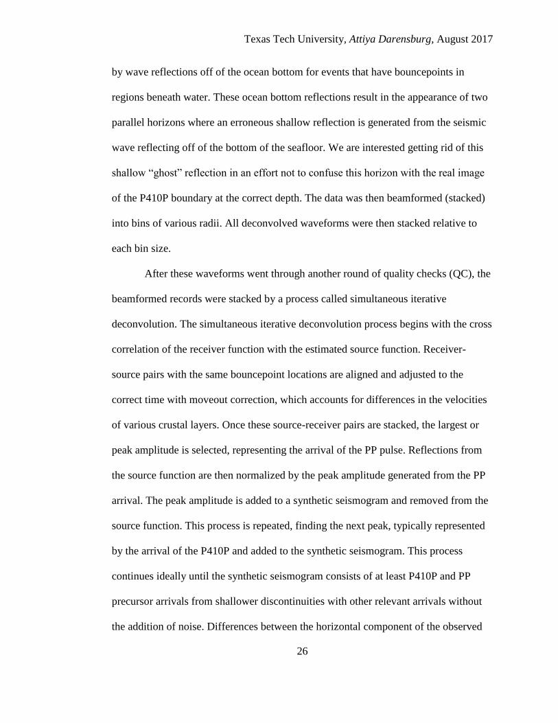
4.1b. Map of the 410 km discontinuity with respect to amplitude at 1Hz.
The amplitudes displayed are measured relative to the main pulse
of the direct PP arrival by normalization at a range between 0 and 0.06 …... 39
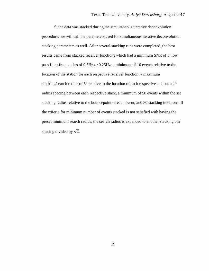
4.1c. Map of the 410 km discontinuity with respect to depth at 0.5Hz.
The depth range is between 370 km and 450 km below the
Earth’s surface …………………………………………………………...…. 39
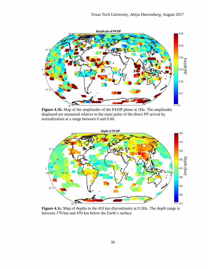
4.1d. Map of the 410 km discontinuity with respect to amplitude at 0.5Hz.
The amplitudes displayed are measured relative to the main pulse
of the direct PP arrival by normalization at a range between 0 and 0.06 .…... 40
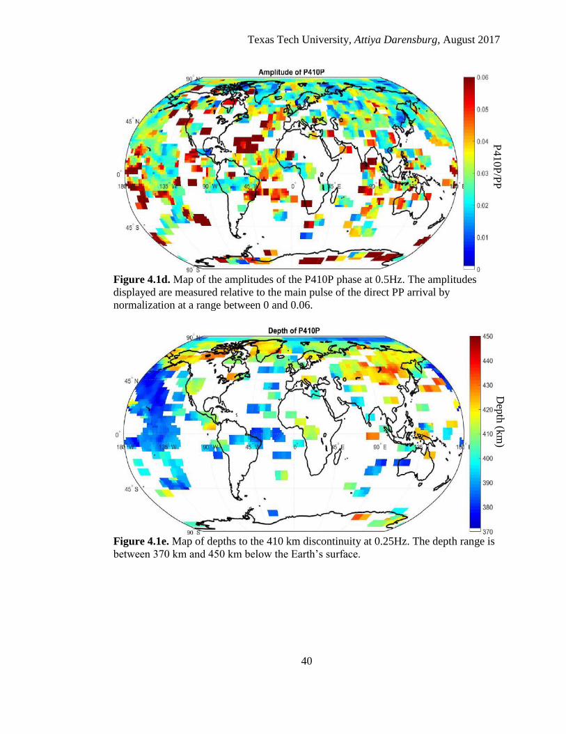
4.1e. Map of the 410 km discontinuity with respect to depth at 0.25Hz.
The depth range is between 370 km and 450 km below the Earth’s
surface ………………………………………………………………………. 40
4.1f. Map of the 410 km discontinuity with respect to amplitude at 0.25Hz.
The amplitudes displayed are measured relative to the main pulse of the
direct PP arrival by normalization at a range between 0 and 0.06 ………...... 41
4.2a. Global distribution of S wave velocity (Vs) perturbations
represented as the percentage of the expected Vs at
400 km depth (~ 4.77 to 4.93 km/s). Unlike Vp, Vs is more
sensitive to temperature variations, as shear wave reflections
vary more immediately when propagating through warmer mantle
environments ………………………………………………………………... 41
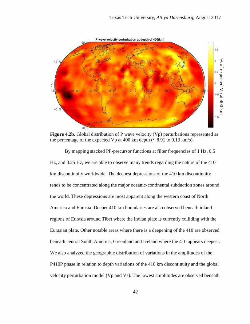
4.2b. Global distribution of P wave velocity (Vp) perturbations represented
as the percentage of the expected Vp at 400 km depth (~ 8.91 to 9.13
km/s) ……..………………………………………………………………….. 42
4.3. Depth of the 410 km discontinuity beneath Hawaii at 1Hz (a)
and 0.5Hz (b). The 410 km discontinuity is slightly elevated to a
depth of approximately 400km beneath the island of Hawaii.
The 410 then appears to deepen toward the northeast. The deepest
410 appears around 420 km depth beneath the island of Kaua’i …………… 44
4.4. Velocity perturbation expressed as the percent of the referenced
S wave velocity (Vs) around 400km (~4.77 to 4.93 km/s).
Hawaii is located toward the center of this figure, where the mantle
velocity in proximity to the 410 is between 1% and 1.5% slower
than the reference Vs ………………………………………………………... 45
4.5. Map of P410P amplitudes beneath Hawaii and the immediate

Texas Tech University, Attiya Darensburg, August 2017
xi
surrounding area at 1Hz(a) and 0.5Hz(b). The average amplitdue
beneath Hawaii ranges between 0.025 and 0.03
(2.5% to 3% of the main PP pulse) for 1Hz and 0.5Hz ……………………. 46
4.6. Depth of the 410 km discontinuity beneath Alaska at 1Hz(a),
0.5Hz(b), and 0.25Hz(c). 410 depth ranges from 430 km – 440 km
beneath Alaska at 1Hz and 0.5 Hz. The 410 appears shallower at
0.25 Hz ……………………………………................................................... 47
4.7. Vs velocity perturbation beneath Alaska at 400 km depth.
There is a fast Vs anomaly observed beneath the Aleutian Islands
up toward the Alaskan mainland to the north/northeast.
Vs in this region is around 1% faster than expected ……………………….. 48
4.8. Map of P410P amplitudes beneath Alaska at 1Hz(a), 0.5Hz(b),
and 0.25Hz(c). For all images, the P410P amplitude observed
beneath Alaska ranges from 0.02 to 0.03. The highest amplitudes
are observed to the south and southwest of the Alaskan mainland ………… 49
4.9. Depth of the 410 km discontinuity beneath Eurasia at 1Hz(a),
0.5Hz(b), and 0.25Hz(c). At 1 Hz, the 410 appears depressed
beneath eastern Russia at around 420 km depth. The 410 is
more uniformly depressed throughout China and eastern Russia
at 420 km depth with the use of PP functions filtered at 0.5 Hz.
There are considerable depressions observed beneath Lake Bikal
and areas to the east at 1 Hz and 0.5 Hz ……………………….……….…… 51
4.10. Vs velocity perturbation beneath Eurasia at 400 km depth.
The fastest P wave velocities are observed beneath southern Japan
and the Sea of Japan at approximately 2% faster than average at depth ……. 52
4.11. Map of P410P amplitudes beneath Eurasia at 1 Hz(a), 0.5 Hz(b),
and 0.25 Hz(c). The amplitude of the P410P pulse beneath Eurasia
is relatively small for the majority of the area with normalized values
between 0.01 and 0.03. Some of the greatest amplitudes are observed
beneath the region north of Lake Baikal …..................................................... 53
4.12. Depth of the 410 km discontinuity beneath NW Europe, Greenland
and Iceland at 1Hz(a) and 0.5 Hz(b). The 410 appears to be right at
410 km below most of Sweden and Norway, with a slight elevation
to around 420 km depth toward the southeastern region of Sweden.
A similar pattern in the depth of the 410 km discontinuity is observed
beneath the United Kingdom and Ireland with a depth range between
410 km and 420 km. The 410 appears at approximately 450 km beneath
Iceland ………………………………………………………………………. 55
Texas Tech University, Attiya Darensburg, August 2017
xii
4.13. Velocity perturbation trends beneath NW Europe, Iceland
and Greenland. Slower S wave velocities are observed
primarily around Iceland where Vs is ~1.5 to 2% slower than
expected at 400 km depth. The faster velocities are present beneath
most of Greenland and NW Europe where Vs is 1% faster than
expected at its fastest ……………………………………………..………… 56
4.14. Map of P410P amplitudes beneath NW Europe, Greenland and
Iceland at 1Hz(a) and 0.5 Hz(b). The P410P pulse beneath Iceland
has a magnitude of approximately 0.03 for both 1 Hz and 0.5 Hz.
The P410P pulse beneath Greenland ranges between 0.01 and 0.02
for both frequencies as well. The amplitude range observed beneath
Finland and Sweden is 0.01 – 0.02 at 0.5Hz, but the amplitude
appears to increase to approximately 0.035 beneath Sweden and parts of
Finland at 1 Hz ………………………………………………………...……. 57
4.15. Depth of the 410 km discontinuity beneath South America at
1 Hz (a) and 0.5 Hz (b). The 410 appears to be depressed
throughout the majority of this region with depth ranges between
420 km and 430 km depth. The cool mantle region to the north
appears to be a data processing error due to the abrupt nature of the
apparent elevation of the 410 km discontinuity. The 410 does appear
to gradually elevate to the east, beneath the south Pacific ………………….. 58
4.16. Velocity perturbation trends beneath South America. Slower S
wave velocities are observed beneath the majority of central
South America where the slower anomaly is ~0.5 to1% faster
than expected at 400 km depth …………………………………………........ 59
4.17. Map of P410P amplitudes beneath South America at 1Hz (a)
and 0.5Hz (b). The average magnitude correlating to the P410P
pulse range between 0.01 and 0.025 throughout most of the
mapped region. A concentration of higher magnitudes are located
along the western coast of this area with a particularly strong P410P
pulse observed in the southwestern region …………………………………. 60
5.1. P-wave tomographic map. The proposed hotspot is seen beneath
Hawaii where the Vp is 0.5% slower than average.
(Nolet et al., 2007) ………………………………………………………….. 63
5.2. Depth profile of Hawaiian islands at 0.5 Hz filter frequency.
Starting from left (southeast) to right (northwest), the 410 appears at
approximately 400 km beneath Hawaii and begins to depress toward
the northwest around Maui …………...…………………………………...... 64

Texas Tech University, Attiya Darensburg, August 2017
xiii
5.3. Transition zone thickness anomaly beneath south-central Alaska.
TZ thickness variations are relative to the average thickness of
250 km. (Yinshuang et al., 2005) ………………………………………….. 66
5.4. Depth profile beneath southern Alaska at 0.5 Hz filter frequency.
Starting from the east(left), moving to the west(right), the 410
is clearly depressed beneath the entire landform. There also appears
to be a consisnent negative velocity layer directly above the 410,
indicative of partial melt. The 410 is highlighted by the bold dashed
line …………….……………………………………………………………. 67
5.5. Depth profile beneath the western end of the Aleutian Island chain
at 0.5 Hz filter frequency. Starting from the island to the south(left)
and progressively moving to the north toward Russia(right),
a possible artifact from the subducting slab is observed by the
negative P wave discontinuity pulse ……………………………………….. 67
5.6. The detached Asian Lithospheric Mantle subducting beneath the
lithosphere of Tibet. (Kind et al., 2002) …………………………….……… 70
5.7. Depth profile beneath India and Tibet at 0.5 Hz filter frequency.
Starting from the south(left), moving roughly to the northeast(right)
across what would be part of the collisional arc stretching into
southern Tibet ………….………………………………………...…………. 71
5.8. Depth profile beneath northeast China at 0.5 Hz filter frequency.
Starting from the south(left), moving to the north/northwest(right).
The 410 is depressed to a depth of approximately 430 km as we
move across northeastern China. The P410P pulse widths begin to
narrow as the profile moves more inland to the northwest.
The 410 km discontinuity is outlined by the black dashed line ………..…… 73
5.9a. Depth profile beneath Iceland at 0.5 Hz filter frequency.
Starting from the west(left), moving to the east(right) ..…………….……… 74
5.9b. Depth profile beneath Iceland at 0.5 Hz filter frequency.
Starting from the southwest(left), moving to the northeast(right) ….………. 75
5.10. Depth profile beneath Greenland at 0.5Hz filter frequency.
Near the northeastern coast, there is a strong negative pulse is
observed below the P410P positive pulses by using the depth profile ……... 76
Texas Tech University, Attiya Darensburg, August 2017
1
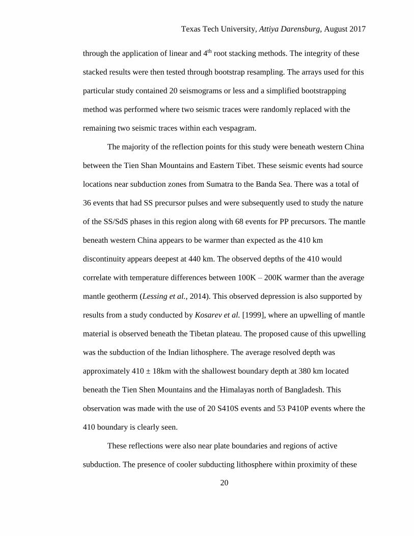
CHAPTER I
INTRODUCTION
The goal of this study is to gain a better understanding of the 410 km discontinuity
(410), which is the discontinuity that defines the upper mantle transition zone (TZ).
The 410 and the TZ in general is considered to be the result of mineral phase changes.
that is generally considered to be bound by mineral phase changes which occur at 410
km depth. The transition zone begins at 410km depth (~14GPa), as a result of the
transformation of olivine (Mg,Fe)2SiO4 into a denser olivine phase called wadsleyite,
also referred to as β-phase olivine or modified spinel (Frost, 2008). The 520km
(~17.5GPa) discontinuity is believed to be the result of wadsleyite (β-phase olivine)
transforming into ringwoodite, which is also referred to as γ-phase olivine or silicate
spinel (Frost, 2008). The final discontinuity defining the base of the transition zone is
observed at 660km depth (~24 GPa). The manifestation of the 660km discontinuity
occurs when ringwoodite breaks down into two separate chemical components,
perovskite (Mg,Fe)SiO3 and magnesiowustite (Mg,Fe)O (Frost, 2008).
The locations of the three major discontinuities were proposed through various
thermodynamic experiments by synthesizing olivine phases at their corresponding
pressure and temperature boundaries using a diamond cell anvil (see Akaogi et al.,
1989). Katsura and Ito (1989) found that the first olivine phase transition begins
around 400 km depth over a depth interval between 9 km to 17 km, where α-
olivine((Mg0.89,Fe0.11)Si2O4) transforms into β-olivine (wadsleyite) at temperatures
between 1400°C – 1600°C (1673K – 1873K). The Clayperon slope is defined by
dP/dT where the change in pressure is measured with respect to the change in

Texas Tech University, Attiya Darensburg, August 2017
2
temperature. The estimated Clayperon slope for the 410km discontinuity was found to
be around 2.5 +/- 1 MPa/K (Katsura et.al, 1989). With a positive Clayperon slope, the
410 km transition boundary is believed to be exothermic. Consequently, the
discontinuity at 410 km tends to be deeper in regions where the mantle is hot (i.e.
where mantle plumes are present) and elevated in cold mantle regions (Flanagan and
Shearer, 1999). The discontinuity at 520 km depth is also thought to be exothermic, so
it has depth variations similar to those found for the 410. The phase transition at 660
km is thought to be endothermic, so depth variations as a function of temperature will
be opposite from the trend observed at the 410.
In an effort to study and understand the complex nature of the transition zone by
tomographic imaging, P (primary) waveforms and, in some instances, S (secondary)
waveforms are used to infer depth variations of discontinuity boundaries within the
upper mantle regions with no seismic stations. The PdP phase (a turning ray that
bounces of the bottom of a velocity boundary at depth “d” and then travels through the
mantle a second time to the recording station) are typically used to image the 410 km
discontinuity (P410P). The P660P phase are typically not observed due to long period
reflections at this depth and due to interference of other phases. The wave path of PP
precursors and direct PP waves are shown in figure 1.1. The following sections will
summarize the previous studies conducted to image the upper mantle at the top of the
transition zone (410 km) using PP precursors. As phase transition boundaries are
thought to be the result of mineral phase changes of olivine as a result of variations in
depth and temperature, the most basic information that we have as to the composition
of the upper mantle are through direct observations regarding the composition of the

Texas Tech University, Attiya Darensburg, August 2017
3
upper mantle from xenoliths in kimberlites or alkali basalts extruded onto the Earth’s
surface (Ringwood, 1991). The known compositions are extrapolated to other mantle
depths by diamond anvil cells and other chemical experiments involving temperature
and pressure changes. As a result, mineral physicists have postulated that the upper
mantle is composed primarily of the mineral olivine with a pyrolytic composition
(Ringwood, 1991).
Figure 1.1. PP precursor reflections off of discontinutiy depths. The variable “d”
represents the depth of underside reflections. (Chambers et al., 2005)
Mineral physicsists found phase changes within a pyrolitic mantle are consistent
with the pressure and temperatures at 410 km, 520 km and 660 km depths (see Akaogi
et al., 1989) which further correlate well with depths found through seismic
observations. The reflection amplitudes of these discontinuities are a function of the
density and velocity contrast across the respective discontinuity (Bina and Helffrich,
1994).

Texas Tech University, Attiya Darensburg, August 2017
4
CHAPTER II
GEOLOGICAL BACKGROUND
Pyrolite vs. Piclogite Mantle
It is important to understand the differences between hypothesized pyrolytic
and piclogitic mantle composition because these two possible mantle types will act
differently in response to pressure and temperature and have different seismic
properties. It is believed that the mantle is composed mostly of olivine, pyroxene(s),
and garnet. The principle rocks which contain these minerals are peridotite (olivine-
rich pyroxene) and piclogite (garnet-rich pyroxene) (Ringwood, 1991). The
composition of the upper mantle is still a topic of debate, but an overwhelming
majority of seismic and laboratory studies (see Ringwood, 1991, Frost, 2008, Akaogi
et al., 1989 and others) support the hypothesis that the mantle is primarily pyrolytic.
Pressure and temperature dependent experiments were conducted in order to
produce estimates for the chemical composition of the upper mantle relationships
between harzburgite and ancient MORB were investigated in a study conducted by
Green et al. [1971] in an effort to constrain the composition of the parental mantle.
The resulting chemical composition is provided in table 2.1.
Texas Tech University, Attiya Darensburg, August 2017
5
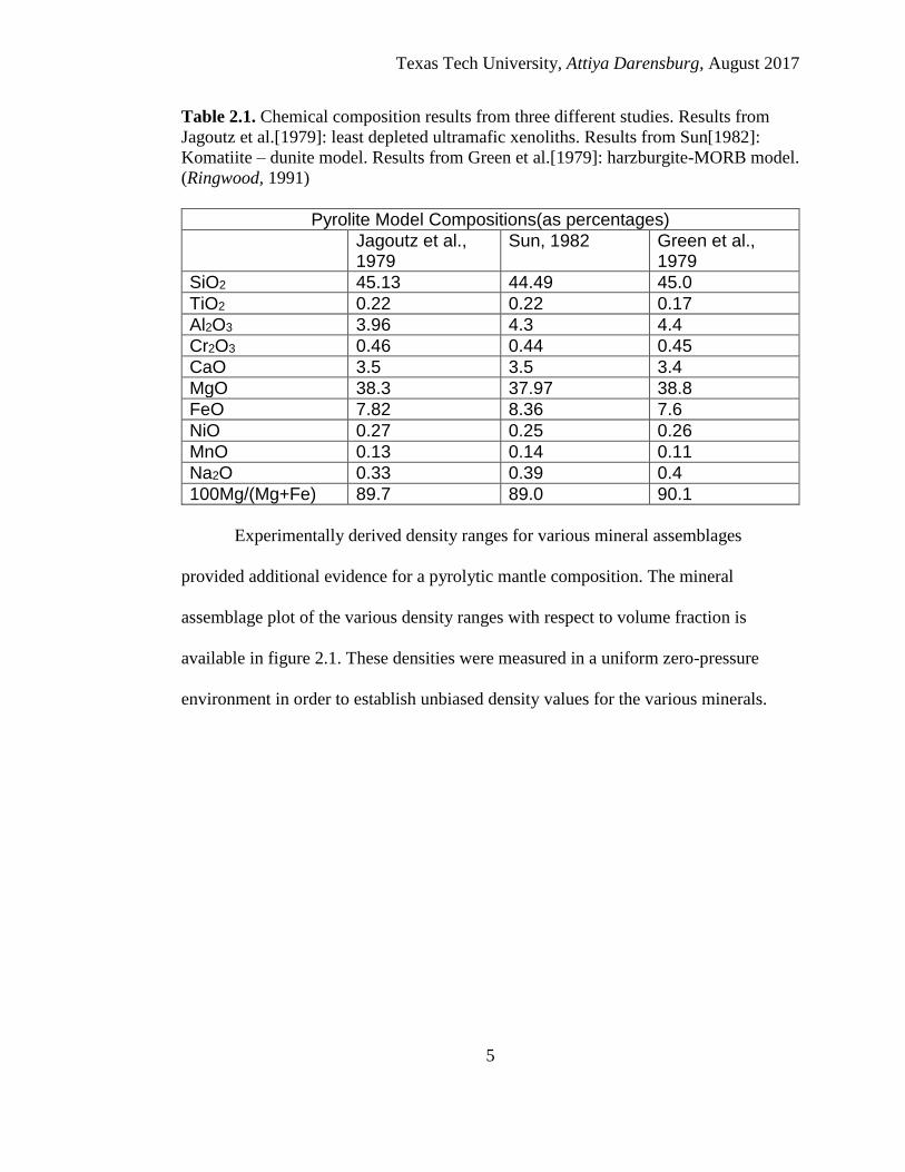
Table 2.1. Chemical composition results from three different studies. Results from
Jagoutz et al.[1979]: least depleted ultramafic xenoliths. Results from Sun[1982]:
Komatiite – dunite model. Results from Green et al.[1979]: harzburgite-MORB model.
(Ringwood, 1991)
Pyrolite Model Compositions(as percentages)
Jagoutz et al., 1979
Sun, 1982 Green et al., 1979
SiO2 45.13 44.49 45.0
TiO2 0.22 0.22 0.17
Al2O3 3.96 4.3 4.4
Cr2O3 0.46 0.44 0.45
CaO 3.5 3.5 3.4
MgO 38.3 37.97 38.8
FeO 7.82 8.36 7.6
NiO 0.27 0.25 0.26
MnO 0.13 0.14 0.11
Na2O 0.33 0.39 0.4
100Mg/(Mg+Fe) 89.7 89.0 90.1
Experimentally derived density ranges for various mineral assemblages
provided additional evidence for a pyrolytic mantle composition. The mineral
assemblage plot of the various density ranges with respect to volume fraction is
available in figure 2.1. These densities were measured in a uniform zero-pressure
environment in order to establish unbiased density values for the various minerals.

Texas Tech University, Attiya Darensburg, August 2017
6
Figure 2.1. The illustration of the composition of the Earth’s upper mantle and
lithosphere. (Ringwood, 1991)
One of the earliest studies by Anderson and Bass [1986] supports the theory that the
upper mantle has a piclogitic composition by comparing mantle composition to the
cosmic abundance of elements that likely contributed to chemical constituents of the
mantle.
Table 2.2. Estimates of the average compositions of subdivisions of the mantle and
the cosmic abundance of elements expressed as wt % oxides. (data taken directly from
Anderson and Bass, 1986)
Cosmic composition (%)
Shallow mantle composition (%)
Transition zone composition (%)
Lower mantle composition (%)
MgO 36.6 42.2 24.0 36.8
CaO 2.89 1.92 8.0 2.4
Al2O3 3.67 2.05 8.6 3.4
SiO2 50.8 44.2 47.0 53.2
FeO 6.08 8.92 10.8 4.8
Anderson and Bass [1986] found that the observed amplitude for seismic
reflections were smaller than those predicted for a pyrolite mantle model. In an
attempt to match the observed velocities at 400 km and 650 km, they assumed a
homogeneous mantle with a garnet to clinopyroxene ratio that matches observed

Texas Tech University, Attiya Darensburg, August 2017
7
velocities in the depth range of 400 km to 550 km. For the lower boundary at 660 km,
they found that the P660P phase velocity spike at this depth could be explained by
piclogite transforming to Mg-perovskite. Ringwood [1991] contradicted Anderson and
Bass [1986] and found that the mantle was better modeled as peridotite with relatively
small localized sections of eclogite dispersed throughout the mantle. Figure 2.1
displays the layered composition of oceanic and continental crust based off of
Ringwood’s hypothesis.
The estimated mineral assemblage for the upper mantle were also derived with
the use of observed P and S wave velocities, which were estimated to an approximate
depth range through data inversion (Ringwood, 1991), and is displayed in table 2.3.
Figure 2.2. Density and depth mineral assemblage plot for pyrolite with respect to
volume fraction. The geotherm near 410 km is assumed to be around 1400°C, while
the geotherm near 660 km is assumed to be around 1600°C in accordance with the
mantle geotherm of Brown and Shankland [1981]. (Ringwood, 1991)

Texas Tech University, Attiya Darensburg, August 2017
8
Table 2.3. P and S wave seismic velocity estimations at 400 km and 650 km
calculated by Kennett [1991]. (Ringwood, 1991)
Seismic parameter P-waves (km/s) S-waves (km/s)
Velocity changes at 400km discontinuity(%)
2.5 – 5.8 2.8 – 5.7
Velocity changes at 650km discontinuity(%)
3.6 – 7.3 3.0 – 7.5
Velocity gradients between 440 – 650 (km/sec)/km
2 × 10⁻³ − 5 × 10⁻³ 1.8 × 10⁻³ − 2.9 × 10⁻³
Many studies have investigated the mantle properties with relation to the ratio of FE to
Mg in the olivine in the mantle (Akaogi et al. [1991], Katsura and Ito [1989] and Ito
and Takahashi [1989]). Brown and Shankland [1981] show the relationship between
mantle pressure and Mg/Fe ratio in the mantle olivine from Akaogi et al. [1989].
Temperature variations and its effects on the depth of various olivine phase boundaries
is shown in figure 2.4. Between figures 2.3 and 2.4 the estimation of the transition
between α-olivine and β-olivine occurring at ~410 km depth and 14 GPa is reasonable.

Texas Tech University, Attiya Darensburg, August 2017
9
Figure 2.3. Phase diagram between the three major olivine mineral phases (olivine (α)
wasleyite (β), wasleyite (β) magnesiowustite and perovskite (γ)) at 1600°C
between 4 GPa and 22 GPa. The shaded rectangle represents the approximate area
where the estimated chemical composition of olivine in the upper mantle is
((Mg0.89Fe0.11)2(SiO4)) (Akaogi, 1989).

Texas Tech University, Attiya Darensburg, August 2017
10
Figure 2.4. Phase boundary diagram for a pyrolytic mantle with variations in
temperature relative to depth. (Akaogi et al., 1989)
Previous studies using seismic waveforms to image discontinuities at 410, 520 and 660 km
Flanagan and Shearer (1998, 1999) stacked P410P and S410S phases from a
global data set and found an average depth for the 410 km discontinuity of 418 – 419
km (see figure 2.5). Regional variations in depth range from 400 km to almost 440
km.

Texas Tech University, Attiya Darensburg, August 2017
11
Figure 2.5. Maps displaying the global topography for the 410 km discontinuity
(Flanagan and Shear, 1999). (a) The result from using P410P waves. (b) The result
from using S410S waves.
These models found deeper than expected for the 410 beneath the Pacific Ocean and
South America in addition to a consistent elevation of the 410 discontinuity beneath
the Indian Ocean and parts of Africa and Antarctica between the P410P and S410S
topographic maps. Flanagan and Shearer found the 410 discontinuity to be absent in
regions with subduction zones and spreading ridges. Lee and Grand [1996] were also
unable to image the 410 beneath the East Pacific rise. Flanagan and Shearer (1998,
1999) found no correlation between depth variations to the 410 and ocean-continent
regions, ruling out the theory that variations in the depth of the 410 could be due to
differences in lithosphere types.
Chambers et al. [2005] found that variations in the P410P and S410S
reflection amplitudes versus S410S reflection amplitudes could be the result of
a)
b)

Texas Tech University, Attiya Darensburg, August 2017
12
variations in water content, the presence of partial melting and chemical
heterogeneities within the mantle. The amplitudes of PP and SS precursors do not rely
solely on impedance contrasts between thermochemical boundaries and the density of
each heterogeneous layer, but they do depend on intrinsic attenuation and anisotropy.
Anisotropy will result in differences in the velocity of seismic waves depending on
which mineral crystalline axis the incoming wave travels along. Intrinsic attenuation
occurs as the result of the structure of the mantle and anisotropy of minerals within the
mantle (Chambers et al., 2005). In his study, the differences in amplitudes have been
interpreted to be a result of changes in discontinuity thickness when short period
waveforms are used. Variations in precursor amplitudes using long period data has
been interpreted to be the likely result of changes in impedance contrasts.
Observations by Vidale and Benz [1997] restricted the thickness of the 410 km
discontinuity to approximately 4 km using a high frequency reflection from that
boundary. This approximation was made citing reflected phases are only sensitive to
impedance gradients less than 1/4th of a wavelength. A study conducted by Rost and
Weber [2002] focused on imaging the transistion zone beneath the western region of
the Pacific Ocean. Their results showed that the 410 km discontinuity must be sharper
than 6 km with a minimum impedance contrast of 6.5%. The 410 has also been
observed to be much thicker, particularly beneath continents. Helffrich and Wood
[1996] found that a 5 km linear impedance gradient can result in reflection coefficients
that are similar to a 10 km nonlinear impedance gradient, which is the case for the
olivine transition between the α and β phases (Stixrude, 1997). van der Meijde et al.
[2003] used receiver functions from reflections beneath Europe to study the

Texas Tech University, Attiya Darensburg, August 2017
13
topography of the 410, where the discontinuity was estimated to be between 25 and 35
km thick. As previously mentioned, variations in the thickness of the 410 km
boundary can be attributed to the amount of water present within the mantle
(Chambers et al. 2005 and Frost, 2008). Water partitions into wadsleyite (β-olivine)
over α-olivine by approximately 10:1 (Wood, 1995), where the β-olivine phase is
more stable at lower pressures. Chen et al. [2002] found that β-olivine is more soluble
in water and therefore corresponds to a phase transition at lower pressures when water
is present. As a result, regions where both α and β phases are stable is broadened and
correlates to an increased presence of water in the mantle. Figure 2.6 shows the effect
that water has on the 410 km discontinuity.
Figure 2.6. This diagram displays the effect water has on the thickness of the
transition boundary between the α and β phases of olivine with water content defined
by weight percentage (wt % ). Notice the broadening effect water has on the thickness
of the discontinuity versus the thickness of the same transition boundary under dry
conditions (Frost, 2008).

Texas Tech University, Attiya Darensburg, August 2017
14
The broadband data used by Chambers et al. [2005] was sampled at a period of
1 second using IRIS, IDA and USGS seismic networks between 1990 and 1999.
Shallow seismic records, events that are 75 km in depth or less and epicentral
distances of 80° – 140° and 100° – 160° for PP and SS waveforms, respectively, were
used to minimize interference with multiple phases. A Butterworth bandpass filter was
applied to both the PP and SS data sets with intervals between 8s to 75s and 15s to 75s
respectively. A Hilbert transform was then applied to the PP data set and the SS data
set was rotated in order to get the transverse component. Data sets with SNR of 3 or
greater and cross correlation coefficients equal to or greater than 0.6 were kept. The
epicentral distance used for the PP data was 110° and 130° for the SS data. This range
was chosen in order to maximize the reflections from the 410 discontinuity while
minimizing interference from other P wave or S wave phases.
The stacks generated for this study were developed by grouping bouncepoints
by 4 different regions (A, B, C, D) around the world, where regions A and D contain
continental bouncepoints and regions B and C contain oceanic bouncepoints (see
figure 2.7).
Figure 2.7. Stacked traces grouped into regions A, B, C and D for the PP data set
(Chambers et al., 2005).

Texas Tech University, Attiya Darensburg, August 2017
15
These regions were selected for the purposes of enhancing the quality of the
stacked midpoints without averaging out the lateral variability. From these stacked
results, the 410 km discontinuity arrival was the clearest and largest feature in the data
sets with an arrival time of approximately 80s. The sidelobes of the P410P arrived
around 100 seconds before the main PP pulse. This sidelobe was separated out with a
deconvolution algorithm. Within each of these regions, there was a noticeable
variation in the amplitudes generated from the reflections off of the underside of the
transition zone. These variations where shown using a frequency histogram where the
amplitudes were measured in 1000 bootstrap samples as shown in figure 2.8.

Texas Tech University, Attiya Darensburg, August 2017
16
Figure 2.8. A) PP precursor stacks from all data and from regions A, B, C and D. The
dashed lines represent 95% confidence limits for the stack determined through
bootstrap resampling. The red curves are stacks of the synthetic seismogram which
include the reference phase and reflections from 220 km, 410 km and 660 km. C)
Display of the depth mapping for PP precursor of all data and regions A, B, C and D.
The width of each bar represents the degree of uncertainty in discontinuity depth.
(Chambers et al., 2005)
The stacked traces for the PP data set shows that the amplitude of the P410P is
higher beneath oceanic regions B and C and lower beneath continental regions A and
D when compared to the amplitudes of the global stack. Figures 2.9a and 2.9b displays
Am
plitu
de relativ
e to m
ain P
P
pulse
Am
plitu
de relativ
e to m
ain P
P
pulse

Texas Tech University, Attiya Darensburg, August 2017
17
the results of stacks using PP precursors beneath continental and oceanic areas. As
previously mentioned, the 410 discontinuity appears to be shallower beneath
continental regions and deeper beneath oceanic regions as cross sections A-a and B-b.
However, results from the stacked SS precursors does not show much variation in the
location of the 410 discontinuity.
Figure 2.9a. Map of cross sections A-a and B-b. (Chambers et al., 2005)

Texas Tech University, Attiya Darensburg, August 2017
18
Figure 2.9b. Tomography of the cross sections labeled in figure 2.11a. Notice
the trend in the location of the P410P beneath Asia and North America versus
the Pacific Ocean. Earlier arrivals of the P410P pulses beneath the Pacific
Ocean are indicative of a depression in the 410 km boundary and vice versa for
the areas beneath Asia and North America. (Chambers et al., 2005)
Observations were also made with the amplitudes of the P410P. These
variations were attributed to lateral heterogeneity within the mantle, which would
directly affect the impedance contrast and cause variations in reflection coefficients.
Since heterogeneity of the mantle has been attributed to the possible presence of water
in the mantle, the hydrated olivine phases would directly affect the bulk modulus and
elastic properties of the mantle. Yusa and Inoue [1997] has shown that the addition of
water to pure Mg-wadsleyite can reduce the bulk modulus of the transition zone by
5% to 11% while Jacobsen et al. [2004] showed that the presence of water at 0.1% wt
in γ-olivine can reduce the impedance of PP precursors by 5.8%.

Texas Tech University, Attiya Darensburg, August 2017
19
Lessing et al. [2014] studied PdP and SdS (focusing on SdS phases) reflections
within the transition zone beneath western China and India. Seismic waveforms with a
maximum deviation of ±5° from the theoretical backazimuth were used in order to
avoid analyzing scattered energy that would arrive at the same time as PP precursors.
Each broadband seismogram was then filtered with a second order Butterworth
bandpass filters with the following corner frequencies: 2s and 20s, 3s and 10s, 5s and
25s, 6s and 50s, 8s and 75s, 15s and 75s, 10s and 100s. These ranges of corner
frequencies were used in order to investigate frequency dependent behavior of the
observed seismic records. Discontinuity depths were derived though a migration
technique used by Thomas and Billen [2009]; Schmerr and Thomas [2011] where
inverse projections from PP and SS precursor pulses to reflection points were
calculated. This process also reduced the size of the Fresnel zone, which improved the
lateral resolution of the stacked results. A 40° by 40° 3D grid was then placed around
theoretical PP/SS bouncepoints with a 1° spacing between each grid. The depth range
for each grid was 0 km to 900 km at a 5 km increment. Travel times for each event
were calculated by ray tracing through the ak135 model (Kennett et al., 1995) from the
source location to the grid point and from the grid point to the receiver location.
Further corrections were made in an effort to account for variations in crustal
structure and lateral heterogeneity of the mantle. SS wave tomography model,
S40RTS (Ritsema et al., 2011), PP wave tomography model, MITP08 (Lee et al.,
2008), and crustal model CRUST2.0 (Bassin et al., 2000) were all used to make
corrections to the travel time calculations. Each seismogram was then subsequently
shifted and stacked by their respective midpoints. The seismograms were stacked
Texas Tech University, Attiya Darensburg, August 2017
20
through the application of linear and 4th root stacking methods. The integrity of these
stacked results were then tested through bootstrap resampling. The arrays used for this
particular study contained 20 seismograms or less and a simplified bootstrapping
method was performed where two seismic traces were randomly replaced with the
remaining two seismic traces within each vespagram.
The majority of the reflection points for this study were beneath western China
between the Tien Shan Mountains and Eastern Tibet. These seismic events had source
locations near subduction zones from Sumatra to the Banda Sea. There was a total of
36 events that had SS precursor pulses and were subsequently used to study the nature
of the SS/SdS phases in this region along with 68 events for PP precursors. The mantle
beneath western China appears to be warmer than expected as the 410 km
discontinuity appears deepest at 440 km. The observed depths of the 410 would
correlate with temperature differences between 100K – 200K warmer than the average
mantle geotherm (Lessing et al., 2014). This observed depression is also supported by
results from a study conducted by Kosarev et al. [1999], where an upwelling of mantle
material is observed beneath the Tibetan plateau. The proposed cause of this upwelling
was the subduction of the Indian lithosphere. The average resolved depth was
approximately 410 ± 18km with the shallowest boundary depth at 380 km located
beneath the Tien Shen Mountains and the Himalayas north of Bangladesh. This
observation was made with the use of 20 S410S events and 53 P410P events where the
410 boundary is clearly seen.
These reflections were also near plate boundaries and regions of active
subduction. The presence of cooler subducting lithosphere within proximity of these

Texas Tech University, Attiya Darensburg, August 2017
21
elevations was proposed as the cause of this phenomena, as the subducting Indian
lithosphere reaches the upper mantle, the boundary at 410 km moves to a shallower
depth. These elevated bouncepoints correspond to a mantle temperature that is 200K –
400K cooler than the average mantle geotherm (Lessing et al., 2014). Although this
particular study did not account for the presence of water in the mantle, placed there
by a hydrated subducting slab, the storage capacity of the olivine to wadsleyite
reaction is not as significant as the water storage capacity of the wadsleyite to
ringwoodite at 520 km or the complex transition of ringwoodite to magnesiowuesite
and magnesium perovskite at 660 km. The presence of water near the 410 km
discontinuity can cause a reduction in the amplitude of either P410P or S410S
reflections in addition to causing increased travel times as a result of the presence of
slower mantle velocities. Water would also release at the 410 km boundary in order to
accommodate for the difference in storage capacities between α-olivine and β-olivine,
causing the occurrence of partial melt directly above the 410 discontinuity. Depending
on the thickness of the partial melt layer, negative pulse reflections can cause an
amplification of the sidelobes to the P410P and S410S precursors, resulting in the
appearance of one positive pulse followed by a negative pulse. Since two separate
pulses were not observed in the stacked images for Lessing’s study, it is unlikely that
there is the presence of a partial melt layer above the 410 km discontinuity. A map of
the observations made for the 410 km discontinuity is displayed in Figure 2.10, where
there is a clear depression of the 410 primarily located in western China and elevations
of the 410 are seen within the proximity of the Indian plate, although there is one
outlier displayed near the Tien Shen Mountains just south of Kazakhstan.

Texas Tech University, Attiya Darensburg, August 2017
22
Figure 2.10. PP and SS precursor reflections off of the underside of the 410 km
discontinuity. Depressions in the 410 are clustered in the western region of China with
elevations located near the subducting Indian plate boundary. Diamonds represent PP
precursors and circles represent the SS precursors. (Lessing et al., 2014)
Figure 2.11. SdS reflection coefficients relative to incidence angles for the 410 km
boundary. The black curve represents olivine to wadsleyite transition zone for a
pyrolytic mantle. The red curve represents reflection coefficients generated from a
synthetic seismogram using the ak135 mantle model (Kennet et al., 1995). The blue
curve represents reflection coefficients generated from a synthetic seismogram using
the PREM mantle model (Dziewonski and Anderson, 1981).

Texas Tech University, Attiya Darensburg, August 2017
23
CHAPTER III
METHODS
Data Processing
Our study started with data acquisition from the Global Seismic Digital
Network (GSDN) by using the IRIS data management service. After sorting through
the data for useable events we were left with over 300,000 PP waveforms to include
for data processing. These seismic records span a total of 25 years from 1990 to 2015
with earthquake magnitudes 6.0 or greater. An epicentral distance range of 60° – 180°
was used in order to minimize the interference between records from multiple local
events. The magnitude of the PP precursor pulses are measured relative to the
magnitude of the main PP pulse.

Texas Tech University, Attiya Darensburg, August 2017
24
Figure 3.1. This is a map of the global data obtained from 1990 – 2015 from every
available seismic recording station provided by the data management center (DMC).
The black dots represent the midpoints (bouncepoints) for every seismic wave. The
red dots indicate the locations of each station, with noticeable coverage throughout the
United States. The blue dots represent the epicenters of the earthquakes. Notice how
the majority of these seismic events are located on or near plate boundaries.
Data processing started with sorting all earthquake data into folders (high, low,
and others). Records with signal to noise ratios (SNR) values of 3 or greater were
labeled as “high” SNR events, records with SNR events between 1.5 and 3 were
labeled as “others”, and records with SNR events of 1.5 or lower were considered to
be “low”. The next step in data processing involved hand picking seismic events with
clear PP arrivals. We selected all high SNR events and enough of the “others” to have
at least 30 reference phases for each earthquake. The raw data was selected for its
clear PP phase and a lack of obvious noise. The data was cut to include 200s before
the PP phase and 90s after and then resampled to a uniform 20 sps (samples per
second). Cross correlation was used to find more events categorized as “others” or

Texas Tech University, Attiya Darensburg, August 2017
25
“low” SNR that would possibly be useable. This was accomplished by keeping any
event with a cross correlation coefficient of 0.6 or greater, with at least 3 reference PP
phases. Waveforms with focal depths greater than 60 km were also eliminated in an
effort to eliminate arrivals from other P wave phases that might interfere with the
P410P. To convert P410P arrival times for all of our selected waveforms to depth, we
raytraced all events by utilizing the 1D PREM velocity model (Dziewonski and
Anderson,1981).
Figure 3.2. Illustration of beamforming seismic records by receiver location. Each
event is cross correlated with other PP functions based on the location of the
corresponding receiver location. The black triangles represent the events that are
within the search radius for cross correlation. The red triangles are outside of the
search radius and therefore will not be considered for cross correlation.
Each waveform was deconvolved by filtered and unfiltered source functions. The
filtered source functions with “wet” bouncepoints are de-oceaned. The term de-
oceaned refers to the process of removing bouncepoint multiples or “ghosts” generated
Texas Tech University, Attiya Darensburg, August 2017
26
by wave reflections off of the ocean bottom for events that have bouncepoints in
regions beneath water. These ocean bottom reflections result in the appearance of two
parallel horizons where an erroneous shallow reflection is generated from the seismic
wave reflecting off of the bottom of the seafloor. We are interested getting rid of this
shallow “ghost” reflection in an effort not to confuse this horizon with the real image
of the P410P boundary at the correct depth. The data was then beamformed (stacked)
into bins of various radii. All deconvolved waveforms were then stacked relative to
each bin size.
After these waveforms went through another round of quality checks (QC), the
beamformed records were stacked by a process called simultaneous iterative
deconvolution. The simultaneous iterative deconvolution process begins with the cross
correlation of the receiver function with the estimated source function. Receiver-
source pairs with the same bouncepoint locations are aligned and adjusted to the
correct time with moveout correction, which accounts for differences in the velocities
of various crustal layers. Once these source-receiver pairs are stacked, the largest or
peak amplitude is selected, representing the arrival of the PP pulse. Reflections from
the source function are then normalized by the peak amplitude generated from the PP
arrival. The peak amplitude is added to a synthetic seismogram and removed from the
source function. This process is repeated, finding the next peak, typically represented
by the arrival of the P410P and added to the synthetic seismogram. This process
continues ideally until the synthetic seismogram consists of at least P410P and PP
precursor arrivals from shallower discontinuities with other relevant arrivals without
the addition of noise. Differences between the horizontal component of the observed

Texas Tech University, Attiya Darensburg, August 2017
27
seismogram and the predicted signal derived from the convolution of the iteratively
updated receiver function and the vertical component of the observed seismogram are
then calculated using the method of least squares minimization until differences are
negligible.

Texas Tech University, Attiya Darensburg, August 2017
28
Figure 3.3. Steps for simultaneous iterative deconvolution. Step 1 (a): the raw receiver
function is cross correlated with the estimated source function. Step 2 (b): the largest
peak is found and normalized by autocorrelation of the source function. Step 3 (c): the
largest peak from the cross correlated records is removed from the cross correlation
and added to the computed receiver function. Step 4 (d): the new computed receiver
function is used to estimate the original data by convolution with the receiver and
source function. Step 5 (e): the convolution is used to replace data in step 1. Steps 6
through 9( (f) to (i)): the process is repeated with another iteration starting again at
step 1. New peaks are added to the computed receiver function until the original earth
response is found with all relevant discontinuities from the raw data without added
noise. (Rogers, 2013)
Texas Tech University, Attiya Darensburg, August 2017
29
Since data was stacked during the simultaneous iterative deconvolution
procedure, we will call the parameters used for simultaneous iterative deconvolution
stacking parameters as well. After several stacking runs were completed, the best
results came from stacked receiver functions which had a minimum SNR of 3, low
pass filter frequencies of 0.5Hz or 0.25Hz, a minimum of 10 events relative to the
location of the station for each respective receiver function, a maximum
stacking/search radius of 5° relative to the location of each respective station, a 2°
radius spacing between each respective stack, a minimum of 50 events within the set
stacking radius relative to the bouncepoint of each event, and 80 stacking iterations. If
the criteria for minimum number of events stacked is not satisfied with having the
preset minimum search radius, the search radius is expanded to another stacking bin
spacing divided by √2.

Texas Tech University, Attiya Darensburg, August 2017
30
Figure 3.4. Illustration of stacking source-receiver pairs by bouncepoint location.
Seismic records are stacked by the location of their bouncepoints relative to other
events within the defined stacking radius (0.5°,1°,2°,4°,8°, or 12°). The black triangles
represent the events that are within the stacking radius. The red triangles are outside of
the search radius and therefore will not be considered for stacking.
Crustal Tests
Due to the fact that our study did not implement a crustal model in our study,
we decided to test how the quality of our data would have changed and assessed
whether the addition of a crustal model would be necessary. A crustal model would
have accounted for changes in the amplitude and shape of the P410P pulse caused by
multiple crustal layers with different Vp values. However, since the P410P never
passes through the crust at its midpoint, the P410P phase itself is not altered by the
crust but in the simultaneous iterative deconvolution we use the PP phase, which does
pass through the crust, will be effected. Therefore, the deconvolved P410P phase
should be altered to some degree by the crust. To determine to what extent we will

Texas Tech University, Attiya Darensburg, August 2017
31
have to compensate for the P410P phase response to crustal structure, we have made a
series of synthetics for different crustal structure and combinations of crustal structure.
We used PREM velocity model (Dziewonski and Anderson,1981) structure and change
the crust in each test. Each test was run with variations in the thicknesses of the crust
using simultaneous deconvolution of 8 different seismograms with different crustal
thicknesses. These tests were repeated at the following frequencies: 2, 1, 0.5, and 0.25
Hz. The first round of tests addressed the effects of differing crustal thicknesses as a
function of frequency on amplitudes of P410P, arrival times of P410P, and amplitude
ratio between P410P and PP (Figure 3.5).
0
0.5
1
1.5
0 2 4 6 8 10 12 14
2 Hz Crust Test
P410P arrival P410P amplitude P410P/PP
Test number
0
0.2
0.4
0.6
0.8
1
1.2
0 2 4 6 8 10 12 14
1 Hz Crust Test
P410P arrival P410P amplitude P410P/PPTest number

Texas Tech University, Attiya Darensburg, August 2017
32
Figure 3.5. P410P amplitudes at 2, 1, 0.5, and 0.25 Hz filter frequencies for
simultaneous deconvolution of 8 synthetic seismograms with each having a crust of
random thickness (between 20 km and 60km). Amplitudes were normalized by the
expected amplitude of the P410P phase. The horizontal axis is the trial number for the
12 tests.
All numerical values are normalized to the mean for each category (i.e.: P410P time,
P410P amplitude, and P410P/PP ratio). The arrival time for the P410P appears to be
unaffected by the presence of a crustal layer at every frequency. This is particularly
important for our results since we can rule out crustal effects for variations in the
depth of the 410 km discontinuity in our results at any frequency. There is, however, a
0
0.2
0.4
0.6
0.8
1
1.2
0 2 4 6 8 10 12 14
0.5 Hz Crust Test
P410P arrival P410P amplitude P410P/PP
0
0.2
0.4
0.6
0.8
1
1.2
0 2 4 6 8 10 12 14
0.25 Hz Crust Test
P410P time P410P amplitude P410P/PP
Test number
Test number

Texas Tech University, Attiya Darensburg, August 2017
33
clear effect on the amplitude of the P410P phase with variations in filter frequencies
and crustal thickness. However, we see that there were only errors in the expected
amplitude for 2 of the 12 trials. These results imply that, for random crustal
thicknesses between 40 and 60 km, we can expect the correct amplitude the majority
of the time. Pulses generated from this PP precursor had noticeably broader pulse
widths and were less robust at lower frequencies in comparison to the sharper PP
precursor spikes observed at 2Hz and 1Hz. A synthetic seismogram for eight
consecutive crustal models, each having a thickness of 30 km, is displayed in figure
3.6. Notice the variation in amplitude and pulse widths between synthetic
seismograms filtered at 2 Hz and 0.25 Hz. Sharper pulses are observed for seismic
records filtered at 2 Hz, while more diffuse and shorter pulses are observed in seismic
records filtered at 0.25 Hz.

Texas Tech University, Attiya Darensburg, August 2017
34
Figure 3.6. Synthetic seismogram using PREM model. Frequency is 2Hz (a) and 0.25
Hz (b) with a sampling rate of 40sps. The reflection corresponding to the P410P
boundary arrives around 87.5 s.
The second round of testing was performed to determine the effect of various crustal
thicknesses on amplitude as a function of frequency. Results from this test are
displayed in figure 3.7 for four different crustal thicknesses of 20, 30, 40 and 50 km
with a 10 km variation for each thickness parameter. Fifty iterations for each average
crustal thickness were performed at filter frequencies of 2, 1, 0.5, 0.25 and 0.125 Hz.
For every iteration, each of the 8 synthetics were produced using 8 different source
functions that were extracted from the data. The precursor arrival time and PP arrival
time are consistent for every iteration regardless of the crustal thickness used or
frequency. So depth estimates should not be significantly affected by crustal thickness.
a)
b)

Texas Tech University, Attiya Darensburg, August 2017
35
The mean amplitude for each P410P arrival is plotted as a single point with error bars.
The error bars are defined as the standard deviation of the 50 amplitude measurements
of the P410P phase from each crustal test. These crustal tests were conducted for
crustal thickness ranges of 20km ± 10km, 30km ± 10km, 40km ± 10km and 50km ±
10km. All of the precursor amplitudes were normalized by the maximum amplitude of
the main PP arrival.
Figure 3.7. Crustal test with 50 iterations at 2Hz (a), 1Hz (b), 0.5Hz (c), 0.25Hz (d)
and 0.125Hz (e). The blue trend-line connects the mean amplitude for 8 crustal layers
at various thickness ranges from 20km±10km, 30km±10km, 40km±10km, and
50km±10km. The black asterisks represent individual P410P amplitudes.
The P410P had errors in the amplitude at all frequencies between 2Hz and
0.5Hz. The amplitudes for P410P vary considerably for filter frequencies between 2Hz
a) b)
c) d)
e)

Texas Tech University, Attiya Darensburg, August 2017
36
and 0.5Hz, with a maximum mean amplitude variation of 0.0064 at 2Hz, 0.0069 at
1Hz, and 0.0068 at 0.5Hz. The best results were observed using filter frequencies of
0.25Hz and 0.125Hz where the amplitudes were the most consistent with smaller
standard deviation values. Although the mean amplitude variation for 0.25 Hz is
comparable to the other mean amplitude corresponding to higher filter frequencies, the
consistency of the individual amplitudes is more pronounce, especially for crustal
thicknesses between 30 km and 50 km, lead us to believe even at these frequencies
P410P amplitudes have value if the crust at the midpoint is normal continental crust
(30 to 40 km). These results could indicate that imaging the 410 could be problematic
at 0.125Hz for events with bouncepoints located in thinner crustal regions, like
oceanic regions or rift zones.

Texas Tech University, Attiya Darensburg, August 2017
37
CHAPTER IV
RESULTS
Analysis on the P410P phase as a function of frequency will help determine the
depth interval of the velocity gradient associated with the 410 km discontinuity, so we
picked the depths and amplitudes for the P410P phase at frequencies of 1, 0.5, and
0.25 Hz (see figures 4.1a through 4.1f). PP-functions were also produced at a low pass
filter frequency of 0.125 Hz. While the resolution of the 0.125 Hz PP-functions was
noticeably cleaner than those produced at 0.5 Hz and 0.25 Hz, the P410P was not
consistently observed and the data density was too sparse for global interpretation
when sampled at a frequency of 0.125 Hz, so these results were not included. Where
data density was high and the quality of the P410P phase was satisfactory, the depths
to the P410P boundary were mapped. There are larger variations in the amplitudes of
the P410P phase, resulting in the appearance of abrupt spikes in pulse amplitudes.
These spikes in amplitude could be attributed to changes in crustal thickness and the
detection of localized variations in the topography of the upper mantle at 410 km
depth, and since the frequency of the data used for our study was higher than those
used in many older studies (which are typically filtered at 0.01Hz), we expect better
resolution.
Maps of P and S wave velocity perturbation at 400 km are displayed in figure
4.2, where Vp and Vs are expressed as the percentages of the expected velocity of the
mantle at 400 km depth, which is approximately between 8.91 to 9.13 km/s and 4.77
to 4.93 km/s, respectively. These maps will be used to determine if there is any
correlation between velocity, amplitdude and depth of the 410 km discontinuity which

Texas Tech University, Attiya Darensburg, August 2017
38
presumably would be related to variations in temperature. Negative percentage values
are indicative of a slower mantle region and positive percentage values are indicative
of a faster mantle region. Overall, Vp appears to be faster beneath continents and
slower beneath areas that are within close proximity to active rift zones, hot mantle
plumes, and subduction zones. However, since shear seismic waves are more sensitive
to temperature variations than P-waves, we will rely more heavily on the Vs velocity
perturbation maps to better understand the significance of the observed depths and the
amplitude variations inferred from P410P phases. The fastest S wave velocities are
observed beneath parts of western Europe, central Africa, southern Japan and
Australia. The slowest S wave velocities are observed beneath areas where high
thermal gradients are found like the East African rift, Iceland, Hawaii and the South
Pacific.
Figure 4.1a. Map of depths to the 410 km discontinuity at 1Hz. The depth range is
between 370 km and 450 km below the Earth’s surface.
Dep
th (k
m)
Texas Tech University, Attiya Darensburg, August 2017
39
Figure 4.1b. Map of the amplitudes of the P410P phase at 1Hz. The amplitudes
displayed are measured relative to the main pulse of the direct PP arrival by
normalization at a range between 0 and 0.06.
Figure 4.1c. Map of depths to the 410 km discontinuity at 0.5Hz. The depth range is
between 370 km and 450 km below the Earth’s surface.
Dep
th (k
m)
P410P
/PP
Texas Tech University, Attiya Darensburg, August 2017
40
Figure 4.1d. Map of the amplitudes of the P410P phase at 0.5Hz. The amplitudes
displayed are measured relative to the main pulse of the direct PP arrival by
normalization at a range between 0 and 0.06.
Figure 4.1e. Map of depths to the 410 km discontinuity at 0.25Hz. The depth range is
between 370 km and 450 km below the Earth’s surface.
Dep
th (k
m)
P410P
/PP

Texas Tech University, Attiya Darensburg, August 2017
41
Figure 4.1f. Map of the amplitudes of the P410P phase at 0.25Hz. The amplitudes
displayed are measured relative to the main pulse of the direct PP arrival by
normalization at a range between 0 and 0.06.
Figure 4.2a. Global distribution of S wave velocity (Vs) perturbations represented as
the percentage of the expected Vs at 400 km depth (~ 4.77 to 4.93 km/s). Unlike Vp,
Vs is more sensitive to temperature variations.
% o
f expected
Vs at 4
00 k
m
P410P
/PP
Texas Tech University, Attiya Darensburg, August 2017
42
Figure 4.2b. Global distribution of P wave velocity (Vp) perturbations represented as
the percentage of the expected Vp at 400 km depth (~ 8.91 to 9.13 km/s).
By mapping stacked PP-precursor functions at filter frequencies of 1 Hz, 0.5
Hz, and 0.25 Hz, we are able to observe many trends regarding the nature of the 410
km discontinuity worldwide. The deepest depressions of the 410 km discontinuity
tends to be concentrated along the major oceanic-continental subduction zones around
the world. These depressions are most apparent along the western coast of North
America and Eurasia. Deeper 410 km boundaries are also observed beneath inland
regions of Eurasia around Tibet where the Indian plate is currently colliding with the
Eurasian plate. Other notable areas where there is a deepening of the 410 are observed
beneath central South America, Greenland and Iceland where the 410 appears deepest.
We also analyzed the geographic distribution of variations in the amplitudes of the
P410P phase in relation to depth variations of the 410 km discontinuity and the global
velocity perturbation model (Vp and Vs). The lowest amplitudes are observed beneath
% o
f expected
Vp at 4
00 k
m

Texas Tech University, Attiya Darensburg, August 2017
43
regions of deeper 410 km discontinuity depths, which are all indicative of the presence
of a warmer mantle region. Cooler mantle regions correspond to shallower 410 km
discontinuity depths and are located primarily beneath the Pacific Ocean and parts of
the Atlantic Ocean. The higher relative amplitudes observed beneath these regions
also support the theoretical presence of a cooler mantle at 410 km depth.
PP-precursor functions beneath Hawaii
A moderately depressed 410 is observed beneath Hawaii, appearing between
410 km and 420 km, with the deepest 410 observed beneath the northern most parts of
the island chain beneath the islands of Kauai and Ni’ihau (see figure 4.3). The mapped
P410P depth using stacks filtered at 0.25Hz was excluded here due to the lack of
coverage.

Texas Tech University, Attiya Darensburg, August 2017
44
Figure 4.3. Depth of the 410 km discontinuity beneath Hawaii at 1Hz (a) and 0.5Hz
(b). The 410 km discontinuity is slightly elevated to a depth of approximately 400km
beneath the island of Hawaii. The 410 then appears to deepen toward the northeast.
The deepest 410 appears around 420 km depth beneath the island of Kaua’i.
Results from our depth analysis agree with previous studies conducted near Hawaii,
one in particular used only half of the currently available transportable array (TA) data
(see Ainiwaer, 2014). Ainiwaer [2014] mapped the 410 beneath Hawaii and found the
boundary to be slightly depressed beneath the northwestern part of the island chain at
approximately 425 km depth for 0.25Hz and 0.5Hz, although the depression is less
pronounced on the 0.5Hz map. Due to the exothermic nature of the 410, this
discontinuity is expected to be deeper beneath warm regions which would suggest a
deeper 410 near Hawaii is related to the hotspot in this region. Using the S wave
velocity perturbation model (Simmons et al., 2011), the mantle at 400 km depth is
a)
b)
Dep
th (k
m)
Dep
th (k
m)

Texas Tech University, Attiya Darensburg, August 2017
45
warmest toward the oldest islands in the northwest where Vs is 1% and 1.5% slower
than the reference Vs.
Figure 4.4. Velocity perturbation expressed as the percent of the referenced S wave
velocity (Vs) around 400km (~4.77 to 4.93 km/s). Hawaii is located toward the center
of this figure, where the mantle velocity in proximity to the 410 is between 1% and
1.5% slower than the reference Vs.
The presence of a warmer mantle is also supported by observations made
through the amplitudes of the stacked P410P pulses. The amplitude of the P410P
precursor arrivals are noticably small with respect to the amplitude of the main PP
arrival, being approximately 2% to 3% of the amplitude of the main PP pulse. The
expected amplitude of the P410P pulse, which is ~0.035, is derived from the velocity
and density contrasts in PREM (Dziewonski and Anderson, 1981). The depth interval
of the velocity gradient at the 410 km discontinuity has also been shown to have an
effect on the amplitude and pulse width of the P410P phase (see Ainiwaer, 2014).
Ainiwaer (2014) found that P410P pulse amplitudes were lower and the pulse was
wider for a simulated 30 km thick velocity gradient at 410 km depth as compared to
the P410P phase for the expected 10 km gradient. Due to the presence of a warmer
mantle beneath Hawaii, the chemical phase chnge from olivine to wadsleyite is
expected to be relatively thin (see Akaogi et al., 1989). Figure 4.5 displays the
%V
s at 40
0 k
m

Texas Tech University, Attiya Darensburg, August 2017
46
amplitdue patterns observed beneath Hawaii using stacked PP functions filtered at 1Hz
and 0.5Hz, respectively. The average amplitdue beneath Hawaii ranges between 0.025
and 0.03 for 1Hz and 0.5Hz, which are lower than the 0.035 value predicted by the
model of the velocity gradient at 410 km depth using PREM (Dziewonski and
Anderson, 1981).
Figure 4.5. Map of P410P amplitudes beneath Hawaii and the immediate surrounding
area at 1Hz(a) and 0.5Hz(b). The average amplitdue beneath Hawaii ranges between
0.025 and 0.03(2.5% to 3% of the main PP pulse) for 1Hz and 0.5Hz.
PP-precursor Functions beneath Alaska
The average depth to the 410 beneath the majority of Alaska is 430 km which
would be indicative of a mantle that is hotter than usual. Even though there are no
known hotspots near Alaska, there is a subduction zone along the western coast where
the Pacific plate is subducting beneath Alaska from the northwest at a rate of 54
mm/yr (Yinshuang et al., 2005). The 410 is particularly deep beneath Alaska, but the
b)
a)
P4
10
P/P
P
P410P
/PP

Texas Tech University, Attiya Darensburg, August 2017
47
410 is shallower (405 km to 410km) to the immediate southeast of the subduction
zone (see figure 4.6). There is also a slight deepening of the 410 to the northwest
between Russia and Alaska. While the depth results appear consistent between the 1
Hz and 0.5 Hz maps, the depth of the 410 km discontinuity appears to vary the most
with stacked PP functions filtered at 0.25 Hz. The velocity perturbation model of the
mantle at 400 km beneath Alaska and the surrounding areas show a fast velocity ano-
maly stretching from the Aleutian island chain in the southwest to the north/northeast,
ending a little more than half way beneath the Alaskan mainland where the Vs
velocity is approximately 1% faster than expected (see figure 4.7).
Figure 4.6. Depth of the 410 km discontinuity beneath Alaska at 1Hz(a), 0.5Hz(b),
and 0.25Hz(c). 410 depth ranges from 430 km – 440 km beneath Alaska at 1Hz and
0.5 Hz. The 410 appears shallower at 0.25 Hz.
a) b)
c)
Dep
th (k
m)
Dep
th (k
m)
Dep
th (k
m)

Texas Tech University, Attiya Darensburg, August 2017
48
Figure 4.7. Vs velocity perturbation beneath Alaska at 400 km depth. There is a fast
Vs anomaly observed beneath the Aleutian islands up toward the Alaskan mainland to
the north/northeast. Vs in this region is around 1% faster than expected.
P410P amplitudes appear to be relatively low (around 0.02) beneath the majority of
Alaska at 1 Hz, with higher amplitudes observed to the southeast of Alaska (around
0.04) and as high as 0.06 to the south (see figure 4.8). The amplitudes vary
considerably for the stacked PP functions filtered at 0.5 Hz, as the average P410P
pulse amplitude is around 0.02 to 0.03 with an anomaly in amplitudes of 0.04 to 0.06
south of Alaska. The results from stacked PP functions filtered at 0.25 Hz has a
considerable variation in amplitude as well. P410P pulse amplitudes are observed to
be around 0.02 beneath most of Alaska, but can be as high as 0.04. Higher amplitudes
are also observed to the south/southwest.
%V
s at 40
0 k
m

Texas Tech University, Attiya Darensburg, August 2017
49
Figure 4.8. Map of P410P amplitudes beneath Alaska at 1Hz(a), 0.5Hz(b), and
0.25Hz(c). For all images, the P410P amplitude observed beneath Alaska ranges from
0.02 to 0.03. The highest amplitudes are observed to the south and southwest of the
Alaskan mainland.
PP-precursor functions beneath Eurasia
The Eurasian plate, particularly beneath eastern most Russia and China, have
significant temperature anomalies in the upper mantle because it is also part of a
subduction zone. This area has two subduction events. To the north, the Pacific plate is
subducting beneath the North American and Eurasian plates. To the south, the
Philippine plate is subducting beneath the Eurasian plate. The depth of the 410 km
discontinuity beneath this region indicate the presence of a warmer mantle beneath the
Eurasian continent and the Sea of Okhotsk, with a progressively cooler mantle to the
east beneath the Pacific Ocean. The depth of the 410 appears to be shallower beneath
a) b)
c)
P4
10
P/P
P
P4
10
P/P
P
P410P
/PP
Texas Tech University, Attiya Darensburg, August 2017
50
Russia with an average depth of ~420 km. The depth observed beneath China is ~430
km for PP functions filtered at 1 Hz (see figure 4.9). The depth of the 410 was more
consistent beneath China and Russia with an average depth of 420 km when PP
functions were filtered at 0.5 Hz. The 410 appears to deepen beneath southwest Russia
and Mongolia to approximately 430 km. The 410 appears deepest beneath Lake Baikal
and the region approximately 15° to the east when PP functions filtered at 0.25 Hz are
used. Although coverage is weakest for PP functions filtered at 0.25Hz beneath
eastern Russia, the 410 is clearly observed to be approximately 420 km deep. The 410
appears to gradually shallow beneath Russia around 135°E and continues to shallow to
depths between 400 km and 410 km at ~105°E to the west. The 410 also appears
elevated beneath southern Kamchatka when PP functions filtered at 1 Hz and 0.5 Hz
were used, but for 0.25 Hz PP functions, the 410 is shallow beneath the entire
peninsula of Kamchatka.

Texas Tech University, Attiya Darensburg, August 2017
51
Figure 4.9. Depth of the 410 km discontinuity beneath Eurasia at 1Hz(a), 0.5Hz(b),
and 0.25Hz(c). At 1 Hz, the 410 appears depressed beneath eastern Russia at around
420 km depth. The 410 is more uniformly depressed throughout China and eastern
Russia at 420 km depth with the use of PP functions filtered at 0.5 Hz. There are
considerable depressions observed beneath Lake Bikal and areas to the east at 1 Hz
and 0.5 Hz.
Velocity perturbations at a depth of 400 km beneath Eurasia are generally fast. The
fastest P and S wave velocity is observed beneath southern Japan and the Sea of Japan
where it is estimated to be around 2% greater than expected. S wave velocities
a)
b)
c)
Dep
th (k
m)
Dep
th (k
m)
Dep
th (k
m)

Texas Tech University, Attiya Darensburg, August 2017
52
observed beneath nearly all of the northeastern region of China show velocity
anomalies that are about 1% to 1.5% greater than average. Vs appears to be close to
average beneath Lake Baikal (see figure 4.10).
Figure 4.10. Vs velocity perturbation beneath Eurasia at 400 km depth. The fastest P
wave velocities are observed beneath southern Japan and the Sea of Japan at
approximately 2% faster than average at depth.
The amplitude of the P410P beneath Eurasia is relatively small for the majority
of the area with amplitudes between 0.01 and 0.03. The highest amplitudes are
observed beneath South Korea and Russia, especially around Lake Baikal. The highest
P410P amplitude is observed on the 0.25 Hz plot, where the amplitude is as high as
0.06 in South Korea and just north of Lake Baikal. The magnitude averages around
0.04 on the 1 Hz and 0.5 Hz plot for the majority of the region beneath Lake Baikal,
with particularly high amplitudes to the north. The amplitude of the P410P reflection
(see figure 4.11) is also greater beneath most of the Kamchatka peninsula, which is in
agreement with the trend observed with the depth of the 410 in figure 4.9.
%V
s at 40
0 k
m

Texas Tech University, Attiya Darensburg, August 2017
53
Figure 4.11. Map of P410P amplitudes beneath Eurasia at 1 Hz(a), 0.5 Hz(b), and
0.25 Hz(c). The amplitude of the P410P pulse beneath Eurasia is relatively small for
the majority of the area with normalized values between 0.01 and 0.03. Some of the
greatest amplitudes are observed beneath the region north of Lake Baikal.
PP-precursor functions beneath northwestern Europe, Greenland, and Iceland
The 410 km discontinuity is deep beneath the north Atlantic from Greenland
through western Europe. The 410 appears to be deepest (~450 km) beneath Iceland,
which is to be expected given the presence of the hot spot beneath Iceland. There is a
a)
b)
c)
P4
10
P/P
P
P410P
/PP
P
410P
/PP

Texas Tech University, Attiya Darensburg, August 2017
54
small area of gradual shallowing of the 410 observed beneath the Norwegian Sea and
appears to be right at 410 km below most of Sweden and Norway, but is slightly
deeper (~420 km) beneath the southeastern region of Sweden. The depth of the 410
km discontinuity beneath the United Kingdom and Ireland is between 410 km and 420
km.
In the 1 Hz map, the 410 shallows beneath most of Greenland, to ~420 km but
is deepest beneath the eastern and northern coasts of Greenland at depth of 430 km.
The 410 also deepens beneath the eastern coast of Greenland. A slightly elevated 410
is observed beneath the northeastern coast of Greenland (~400km) at 0.5 Hz. Depths
to the 410 for the 0.25 Hz results generally agree with the 0.5 Hz and 1 Hz results
except beneath Iceland. Instead, the 410 appears to be right at 410 km depth in the
0.25 Hz image beneath Iceland. The rest of the region was not data rich enough at
0.25Hz. Due to this discrepancy, results from 1 Hz and 0.5 Hz will be displayed for
the depth plots since these plots had higher data density in this area, and is in
agreement with the known thermal anomalies inferred beneath Iceland from velocity
anomalies. The temperature of the mantle at 410 km depth appears to decrease toward
the south at approximately 60°N latitude.

Texas Tech University, Attiya Darensburg, August 2017
55
Figure 4.12. Depth of the 410 km discontinuity beneath NW Europe, Greenland and
Iceland at 1Hz(a) and 0.5 Hz(b). The 410 appears to be right at 410 km below most of
Sweden and Norway, with a slight elevation to around 420 km depth toward the
southeastern region of Sweden. The 410 appears at approximately 450 km beneath
Iceland.
S wave velocities are shown in figure 4.13 and as expected, the mantle
temperature beneath Iceland is relatively warm, where Vs is ~2% slower than
expected at 400 km. The S wave velocity gradually increases to the south until Vs is
~1% faster than expected beneath the north Atlantic Ocean. S wave velocity anomalies
compliment the pattern observed in the depth plot beneath Greenland as well, as Vs is
slightly faster than the expected velocity along the eastern coast, and becomes
progressively faster inland where Vs is at most 1% faster than expected. There appears
to be no real velocity anomaly beneath Finland, but the Vs beneath Sweden appears to
a)
b) D
epth
(km
) D
epth
(km
)

Texas Tech University, Attiya Darensburg, August 2017
56
be approximately 1% faster than expected. There appears to be no real velocity
anomaly beneath Finland, but the Vs beneath Sweden appears to be approximately 1%
faster than expected.
Figure 4.13. Velocity perturbation trends beneath NW Europe, Iceland and
Greenland. Slower S wave velocities are observed primarily around Iceland where Vs
is ~1.5 to 2% slower than expected at 400 km depth. The faster velocities are present
beneath most of Greenland and NW Europe where Vs is 1% faster than expected at its
fastest.
Amplitude trends for P410P reflections correlate with respect to mantle
temperatures inferred from regional depths of the 410 km discontinuity. The relative
amplitude of the P410P beneath Iceland was around 0.03 at 1 Hz and 0.5 Hz. The
lowest observed amplitudes were found beneath Greenland and parts of Finland. The
amplitudes beneath Greenland and Finland are lower than observed beneath Iceland
where the mantle is much warmer, the P410P amplitudes correlate with the
tomography of the upper mantle at the 410 km discontinuity. The average amplitude
beneath the coast of Finland is around 0.01 to 0.02. Greenland has the same
approximate range as Finland, although, the lower amplitude values at 0.5 Hz extend
%V
s at 40
0 k
m

Texas Tech University, Attiya Darensburg, August 2017
57
farther inland into Sweden. The average amplitude observed beneath Sweden is
approximately 0.035 at 1 Hz.
Figure 4.14. Map of P410P amplitudes beneath NW Europe, Greenland and Iceland at
1Hz(a) and 0.5 Hz(b). The P410P pulse beneath Iceland has a magnitude of
approximately 0.03 for both 1 Hz and 0.5 Hz. The P410P pulse beneath Greenland
ranges between 0.01 and 0.02 for both frequencies as well. The amplitude range
observed beneath Finland and Sweden is 0.01 – 0.02 at 0.5Hz, but the amplitude
appears to increase to approximately 0.035 beneath Sweden and parts of Finland at 1
Hz.
PP-functions beneath South America
The 410 km discontinuity appears to be deep beneath the center of South
America, 420 km and 430 km, from Peru to Brazil at 1 Hz and 0.5 Hz. Depths picked
from PP functions filtered at 0.25 Hz are shallower, between 380 km and 400 km for
P4
10
P/P
P
P410P
/PP
a)
b)

Texas Tech University, Attiya Darensburg, August 2017
58
the same area. However, the data density of this region at 0.25 Hz is also sparse, so
these results are not likely to be reliable.
Figure 4.15. Depth of the 410 km discontinuity beneath South America at 1 Hz (a)
and 0.5 Hz (b). The 410 appears to be depressed throughout the majority of this region
with depth ranges between 420 km and 430 km depth. The cool mantle region to the
north appears to be a data processing error due to the abrupt nature of the apparent
elevation of the 410 km discontinuity. The 410 does appear to gradually elevate to the
east, beneath the south Pacific.
S wave velocity anomalies beneath South America do not correlate as well with the
mapped depth results for the 410 for the most part. The Vs beneath this region are as
much as 1% faster than expected. Small areas on the map show no apparent velocity
anomalies (see figure 4.16).
Dep
th (k
m)
Dep
th (k
m)
a
)
b
)

Texas Tech University, Attiya Darensburg, August 2017
59
Figure 4.16. Velocity perturbation trends beneath South America. Slower S wave
velocities are observed beneath the majority of central South America where the
slower anomaly is ~0.5 to1% faster than expected at 400 km depth.
The amplitude of the P410P reflection beneath this region is relatively small in
the region where velocity anomalies infer a warmer mantle (see figure 4.17). The
amplitude from the 1 Hz PP functions are between 0.01 and 0.025 beneath the
majority of the region. The average amplitude is 0.04 beneath the western coast of
South America. The largest P410P reflection, with an amplitude of 0.05, is observed in
the southwestern portion of this region. The mapped amplitude using 0.5 Hz PP
functions shows the same general pattern observed in the 1 Hz map with a few
exceptions. The amplitude of the P410P reflection observed beneath the western coast
at 1 Hz was not only greater in amplitude, but extended further inland beneath what
would be the western region of Brazil, where the range of amplitude is between 0.02
and 0.03. The peak P410P amplitudes are still located around the southwestern portion
of the mapped region at 0.5 Hz, but the pulse amplitudes can be as high as 0.06. P410P
pulse amplitudes remain small beneath the south Pacific.
%V
s at 40
0 k
m

Texas Tech University, Attiya Darensburg, August 2017
60
Figure 4.17. Map of P410P amplitudes beneath South America at 1Hz (a) and 0.5Hz
(b). The average magnitude correlating to the P410P pulse range between 0.01 and
0.025 throughout most of the mapped region. A concentration of higher magnitudes
are located along the western coast of this area with a particularly strong P410P pulse
observed in the southwestern region.
P410P
/PP
P
410P
/PP
a
)
b
)
Texas Tech University, Attiya Darensburg, August 2017
61
CHAPTER V
DISCUSSION
Analysis of global variations in the 410 km discontinuity using PP precursors
The PP functions that were computed from seismic events mapped in figure
3.1 provided a means for studying the nature of the 410 km discontinuity on a global
scale. We focus here on patterns in depth and amplitude variations estimated from
analysis of P410P phases. We see a significant depression of the 410 (as much as 450
km) beneath all of Iceland, where a known hotspot exists (see Vink, 1984). There are
also some zones that seem contradictory to the hypothesized exothermic behavior of
the 410 km discontinuity, most notably beneath much of northeastern China. The 410
km discontinuity appears to be deeper (~430 km) beneath northeastern China, despite
the fact that the mantle region is thought to be cooler due to the subduction of the
Phillipine plate beneath the Eurasian plate (Li and Yuan, 2003). A possible cause of
this region being warm despite the presence of a subducting slab is the accumulation
of mélange from the Philippine plate at the 660 (Suetsugu et al., 2010), which could
drive a local convection cell that would warm the 410 (see Zhao et al. [2012] and
Duan et al. [2009]). Another possibility for the warming of the 410 is the presence of
partial melt due to mantle hydration from the subducted Philippine plate.
PP precursor amplitudes in many areas appear to correlate with depth
anomalies but there are some notable exceptions. The 410 is a boundary where density
and seismic velocity of the mantle increases quickly over a small enough interval to
cause seismic reflections. This velocity change, however, occurs as a gradient over a

Texas Tech University, Attiya Darensburg, August 2017
62
small interval whose depth ranges can change depending on the temperature of the
mantle. For example, the P410P phase amplitudes are expected to be larger and
narrowed due to a narrow velocity gradient in the mantle in warm regions (see
Ainiwaer, 2014), which is observed to some degree beneath regions like Iceland, NE
China and Hawaii. Otherwise, patterns in the amplitude of P410P reflections vary
somewhat haphazardly throughout the globe with some patterns of high P410P
amplitudes being observed roughly near the mid-Atlantic Oceanic Ridge,
west/southwest of Hawaii, and the southwestern Pacific. These observations roughly
agree with P410P and S410S amplitude trends in the study conducted by Chambers et
al. [2005], where higher S410S amplitudes were observed beneath the south Pacific,
north/northwest of Hawaii and along the mid-Atlantic Oceanic Ridge. Although
Chambers et al. [2005] amplitude results from P410P reflections vary noticeably,
higher P410P amplitudes are observed along the Nazca Ridge, along the southeastern
African coast, east of Hawaii and west of Hawaii for our study. Low P410P reflections
appear beneath the majority of most continents like Russia, northeastern China, and
the middle of South America. Our low P410P reflection trends are in agreement, for
the most part, with the P410P and S410S analysis by Chambers et al. [2005] with the
exception of South America. The following sections will focus on specific regions
were the degree of data coverage is relatively high and are in proximity to major
tectonic events and geological features.
Hawaii
We found that the depth to the 410 beneath the area surrounding Hawaii is
greater than 415 km which is generally deeper than expected (see figure 4.3). The

Texas Tech University, Attiya Darensburg, August 2017
63
deepest observed 410 is in the northwest direction along the island chain (~420 km).
This is consistent with a P410P bouncepoint study by Duncan (2012) using only half
the data that is currently available from the transportable array (TA). The work
presented here includes all the TA stations and any other global seismic stations with
data available through the IRIS DMC. Nolet et al. [2007] observed a low velocity
anomoly to the north of the Hawaiian island chain, tilting to the south from the surface
down to the core-mantle boundary (CMB). The P-wave tomographic map is shown in
figure 5.1, where Vp beneath Hawaii is 0.05% slower than average. But the S-wave
velocities imaged beneath the region at 400 km depth in the GYPSUM model
(Simmons et al, 2011) are ~0.5 to 1% lower then those of PREM which would be
consitent with only a small regional increase in temperature and the small degree of
deepening in the 410 that we observe.
Figure 5.1. P-wave tomographic map. The proposed hotspot is seen beneath Hawaii
where the Vp is 0.5% slower than average. (Nolet et al., 2007)
Figure 5.2 is a depth profile that starts in the Pacific Ocean, southwest of the
main Hawaiian island, and crosses beneath the island chain ending to the northwest of
Kaua’i. The P410P phase appears at ~400 km depth through a series of larger sharp
spikes with narrow pulse widths. As the profile moves across the islands a slight
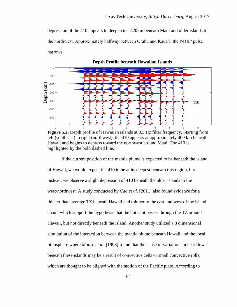
Texas Tech University, Attiya Darensburg, August 2017
64
depression of the 410 appears to deepen to ~420km beneath Maui and older islands to
the northwest. Approximately halfway between O’ahu and Kaua’i, the P410P pulse
narrows.
Figure 5.2. Depth profile of Hawaiian islands at 0.5 Hz filter frequency. Starting from
left (southeast) to right (northwest), the 410 appears at approximately 400 km beneath
Hawaii and begins to depress toward the northwest around Maui. The 410 is
highlighted by the bold dashed line.
If the current position of the mantle plume is expected to be beneath the island
of Hawaii, we would expect the 410 to be at its deepest beneath this region, but
instead, we observe a slight depression of 410 beneath the older islands to the
west/northwest. A study conducted by Cao et al. [2011] also found evidence for a
thicker than average TZ beneath Hawaii and thinner to the east and west of the island
chain, which support the hypothesis that the hot spot passes through the TZ around
Hawaii, but not directly beneath the island. Another study utilized a 3 dimensional
simulation of the interaction between the mantle plume beneath Hawaii and the local
lithosphere where Moore et al. [1998] found that the cause of variations in heat flow
beneath these islands may be a result of convective cells or small convective rolls,
which are thought to be aligned with the motion of the Pacific plate. According to
Depth Profile beneath Hawaiian Islands
Dep
th (
km
)
410

Texas Tech University, Attiya Darensburg, August 2017
65
Moore et al. [1998] the convective cells can cause localized thinning of the
lithosphere, which effectively leads to temperature variations within the
asthenosphere, correlating with the observed trend of a slightly deeper 410 km
discontinuity beneath Hawaii. Results for our study, however, more consistently aligns
with the findings of Cao et al. [2005], where the hotspot is not directly beneath
Hawaii, but is instead located closer to the older islands to the northwest.
Alaska and the Aleutian Islands
The Aleutian islands were formed as a result of the Pacifc plate subducting
beneath the North American plate. Subduction zones tend to cause the surrounding
mantle to become cooler due to the presence of a relatively cooler subducting slab.
Water trapped within hydrated minerals and pore spaces of a subducting oceanic plate
can cause partial melting in the surrounding mantle (Hyndman and Peacock, 2003)
which leads to the formation of a volcanic arc. Although the Aleutian Island chain is
known to be the product of forearc volcanism, the warmest mantle region is observed
beneath Alaska, where the highest depression of the 410 km discontinuity is located
beneath the eastern and northern areas of this region. Alternatively, the coolest mantle
region is observed beneath the Aleutian islands where the 410 is elevated to a depth of
approximately 400 to 405 km (see figure 4.6).
The depression of the 410 beneath Alaska could be correlated to local thinning
of the transition zone (see figure 5.3). Yinshuang et al. [2005] mapped variations in the
thickness of the transition zone beneath the south-central region of Alaska and
generally found thinning of the TZ, by as much as 30 km, beneath this region. Thinner
transition zones correlate to the presence of warmer manle regions due to the
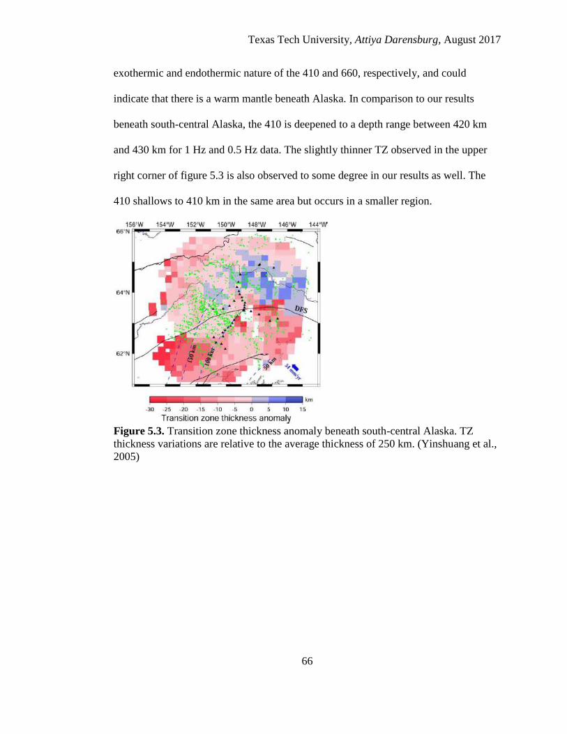
Texas Tech University, Attiya Darensburg, August 2017
66
exothermic and endothermic nature of the 410 and 660, respectively, and could
indicate that there is a warm mantle beneath Alaska. In comparison to our results
beneath south-central Alaska, the 410 is deepened to a depth range between 420 km
and 430 km for 1 Hz and 0.5 Hz data. The slightly thinner TZ observed in the upper
right corner of figure 5.3 is also observed to some degree in our results as well. The
410 shallows to 410 km in the same area but occurs in a smaller region.
Figure 5.3. Transition zone thickness anomaly beneath south-central Alaska. TZ
thickness variations are relative to the average thickness of 250 km. (Yinshuang et al.,
2005)
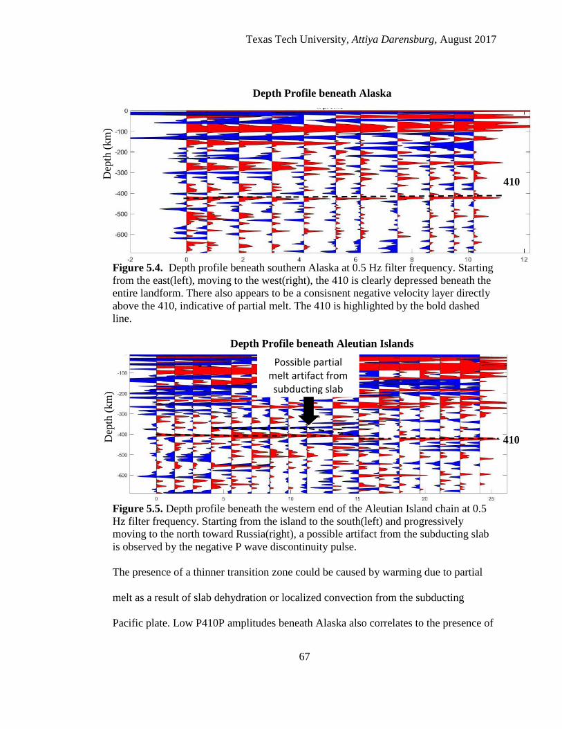
Texas Tech University, Attiya Darensburg, August 2017
67
Figure 5.4. Depth profile beneath southern Alaska at 0.5 Hz filter frequency. Starting
from the east(left), moving to the west(right), the 410 is clearly depressed beneath the
entire landform. There also appears to be a consisnent negative velocity layer directly
above the 410, indicative of partial melt. The 410 is highlighted by the bold dashed
line.
Figure 5.5. Depth profile beneath the western end of the Aleutian Island chain at 0.5
Hz filter frequency. Starting from the island to the south(left) and progressively
moving to the north toward Russia(right), a possible artifact from the subducting slab
is observed by the negative P wave discontinuity pulse.
The presence of a thinner transition zone could be caused by warming due to partial
melt as a result of slab dehydration or localized convection from the subducting
Pacific plate. Low P410P amplitudes beneath Alaska also correlates to the presence of
Dep
th (
km
) D
epth
(km
)
Depth Profile beneath Aleutian Islands
410
Possible partial melt artifact from subducting slab
410
Depth Profile beneath Alaska

Texas Tech University, Attiya Darensburg, August 2017
68
a slow velocity layer found on the subducting slab beneath Alaska in a study
conducted by Yinshuang et al. [2005]. The persistent negative velocity anomoly
observed directly on top of the positive P410P pulse in figure 5.5 is indicative of the
presence of partial melt which supports the hypothesis that the mantle is warm due to
local hydration of the mantle from the subducting slab.
Eurasia and N. India
The next region of interest was mapped in a data rich area of the eastern
Eurasia, from northern Russia to eastern China. The 410 appears to be depressed
beneath northeastern Russia, where the Pacific plate subducts beneath NE Russia and
China, and inland towards Mongolia and the Lake Baikal rift zone (see figure 4.9).
The 410 km discontinuity shallows back up to 410 km beneath the southern tip of
Kamchatka. Since there is nothing more than a transform fault in the Kamchatka
pennisula, there is no current tectonic activity that would not contribute to a change in
the temperature the upper mantle at all (see Chapman and Solomon [1976]).
An increase in the depth of the 410 to ~440 km beneath the Lake Baikal rift
zone (see Gao et al., 2003) suggests that this rift could be driven by magma rising
from a mantle plume, making this an active rift zone. Gao et al. [2003] found the
Baikal rift, created by the rifting of the Siberian and Amurian microplates, to be one of
the most active rift zones in the world, where the thickness of the continental crust is
estimated to be reduced by no more than 5 km. However, other researchers believe
that the Baikal Rift is a passive rift caused by the crustal extension related to the
collision between Eurasia and India (see Petit et al. [1997]). Our results, however,
support the hypothesis that there is a warmer mantle beneath Lake Baikal (see figure

Texas Tech University, Attiya Darensburg, August 2017
69
4.9). To cause a significant warming of the upper mantle, additional geologic
processes must be occurring as vertical mantle upwelling was found beneath Lake
Baikal in a study by Gao et al. [2003]. Evidence supporting a deep source for the
Baikal rift include: observations from bouguer anomaly modeling that the lithosphere
above the rift zone has been uplifted due to vertical mantle convection (Gao et al.
[2003] and Zorin et al. [2003]); and observations of seismic anisotropy which inferred
that the observed vertical alignment of the olivine crystals along the mineral’s fast axis
is the result of mantle upwelling (Gao et al. [2003]). North of Lake Baikal, the 410 is
elevated to the expected nominal depth of 410 km between approximately 85°E to
135°E. This gradual cooling of the mantle can be attributed to the fact that this region
is composed of relatively old lithosphere with no significant temperature anomalies.
A vast area beneath Mongolia and Tibet also appears to have a warmer than
usual mantle, as the 410 appears as deep as 440 km beneath some areas. Seismic and
orogenic activity in the Indian subcontinent and Tibet, are the products of the Indian
plate colliding into the Eurasian plate. Kind et al. [2002] mapped the discontinuity of
the 410 and 660 beneath the Himalayan plateau using data from two profiles across
Tibet. Kind et al. [2002] found evidence supporting the presence of the Tethyan plate,
an older oceanic slab, which would have detached from the India plate. This slab
subduction may cause the surrounding mantle to become progressively warmer over
millions of years due to partial melt caused by dehydration of the slab. This is a
reasonable hypothesis since Kind et al. [2002] mapped a subducting slab beneath Tibet
in their results (see figure 5.6), where they refer to this slab as the detached Asian
Lithospheric Mantle (ALM).

Texas Tech University, Attiya Darensburg, August 2017
70
Figure 5.6. The detached Asian Lithospheric Mantle subducting beneath the
lithosphere of Tibet. (Kind et al., 2002)
Another study conducted by Li et al. [2006] imaged a subducting slab as well, but
theorized that part of the Indian slab is subducting along with the older Tethyan plate.
Figure 5.7 shows our depth profile beneath northern India and southern Tibet from
P410P observations. Although the detached ALM is not seen in this profile, the
negative amplitude anomaly directly above and below the 410 could be the result of a
reflection off of partial melt due to the migration of water to the 410 from the Tethyan
plate.

Texas Tech University, Attiya Darensburg, August 2017
71
Figure 5.7. Depth profile beneath India and Tibet at 0.5 Hz filter frequency. Starting
from the south(left), moving roughly to the northeast(right) across what would be part
of the collisional arc stretching into southern Tibet. The P410P is not only deep, but it
appears to be flanked by low velocity layers above and below. This could be indicative
of the presence of continent crust below and partial melt above.
The next area of interest is northeast China where the Philippine plate is
subducting beneath the Eurasian plate to the south. The P410P pulse widths appear to
narrow toward the northwest. The presence of water has been hypothesized to narrow
the width of the 410 km discontinuity (see Chen et al., 2002). Frost et al. [2007],
however, hypothesized that the presence of water will broaden the mineral phase
change interval at 410 km since water will preferentially partition into wadsleyite. The
abundance of iron could be a possible cause for a narrowed transition boundary at the
410 km as well, leading to a sharper P410P reflection. Although the bulk modulus of
β-olivine is thought to increase with an increase in iron content, an increase in the bulk
modulus would result in only a slight increase in the P-wave velocity gradient between
α-olivine and wadsleyite (Sinogeikin et al., 1998). Iron content in olivine is also
thought to decrease under higher pressures due to the formation of relatively iron rich
Depth Profile beneath northern India and southern Tibet
Dep
th (
km
)

Texas Tech University, Attiya Darensburg, August 2017
72
majorite garnet (Irifune and Isshiki, 1998), effectively reducing the pressure interval
between α-olivine and β-olivine (wadsleyite), and narrowing the phase change interval
between α-olivine and wadsleyite.
Whether the subducting slab is penetrating the base of the 660 or stagnant,
both processes can result in the cooling of the surrounding mantle, which would result
in the elevation of the 410. An argument could also be made for the possibility of a
warmer mantle region closer to 410 km since the dehydration of the Philippine plate
would cause partial melting. Depth anomalies associated with the α – β olivine
transition zone could also be attributed to remnant chemical heterogeneities from the
subducting slab (Li and Yuan, 2003) or mantle plume generation through re-heated
peridotite layers that have accumulated from stagnant slabs (Ringwood, 1991).
Although the Vp and Vs anomolies observed beneath northeastern China at 400 km
depth was faster by approximately 1% of the expected P wave and S wave velocity,
respectively, around 400 km according to Chambers et al. [2005], our results show
that there is a warmer mantle at the 410 km boundary as the 410 appears around 430
km at the deepest along the northeastern coast of China. This apparent contradiction
will require further investigation.
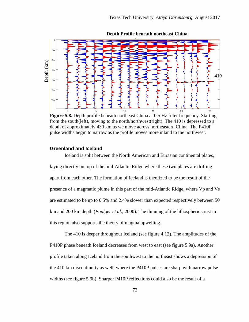
Texas Tech University, Attiya Darensburg, August 2017
73
Figure 5.8. Depth profile beneath northeast China at 0.5 Hz filter frequency. Starting
from the south(left), moving to the north/northwest(right). The 410 is depressed to a
depth of approximately 430 km as we move across northeastern China. The P410P
pulse widths begin to narrow as the profile moves more inland to the northwest.
Greenland and Iceland
Iceland is split between the North American and Eurasian continental plates,
laying directly on top of the mid-Atlantic Ridge where these two plates are drifting
apart from each other. The formation of Iceland is theorized to be the result of the
presence of a magmatic plume in this part of the mid-Atlantic Ridge, where Vp and Vs
are estimated to be up to 0.5% and 2.4% slower than expected respectively between 50
km and 200 km depth (Foulger et al., 2000). The thinning of the lithospheric crust in
this region also supports the theory of magma upwelling.
The 410 is deeper throughout Iceland (see figure 4.12). The amplitudes of the
P410P phase beneath Iceland decreases from west to east (see figure 5.9a). Another
profile taken along Iceland from the southwest to the northeast shows a depression of
the 410 km discontinuity as well, where the P410P pulses are sharp with narrow pulse
widths (see figure 5.9b). Sharper P410P reflections could also be the result of a
Depth Profile beneath northeast China
410
Dep
th (
km
)

Texas Tech University, Attiya Darensburg, August 2017
74
smaller velocity gradient between α-olivine and wadsleyite as this boundary tends to
thin at higher temperatures (see figure 2.4).
Figure 5.9a. Depth profile beneath Iceland at 0.5 Hz filter frequency. Starting from
the west(left), moving to the east(right). The 410 remains depressed throughout this
depth profile. As the profile moves to the east, the P410P pulse amplitude
progressively decreases. A persistent low velocity layer is also present directly above
the 410 discontinuity.
Depth Profile beneath Iceland (West to East)
Dep
th (
km
)
410

Texas Tech University, Attiya Darensburg, August 2017
75
Figure 5.9b. Depth profile beneath Iceland at 0.5 Hz filter frequency. Starting from
the southwest(left), to the northeast(right). This profile taken along Iceland was closer
to the western end of the landform. The P410P pulses are sharp and depressed to ~450
km depth. There also appears to be a persistent low velocity layer above and below the
discontinuity, possibly caused by mantle upwelling.
The 410 is depressed beneath parts of Greenland as well, where the deepest
410 is mapped along the southeastern coast (see figure 4.12). Near the northern coast
of Greenland, a strong negative pulse is observed above and below the P410P positive
pulses in figure 5.10. The P410P phase also appears to reduce in amplitude in the same
area. The remnant warming of the mantle observed beneath Greenland in our study
aligns with the theorized hotspot track traced by Lawver and Muller [1994], where the
residual warming of the upper mantle via Iceland’s hotspot can be seen beneath central
Greenland and the eastern coastline (see figure 4.12). The region closer to Iceland is
likely to have a higher than normal mantle temperature since the mid-Atlantic Ridge
and the hotspot are in the vicinity.
Depth Profile beneath Iceland (Southwest to Northeast)
410 Dep
th (
km
)
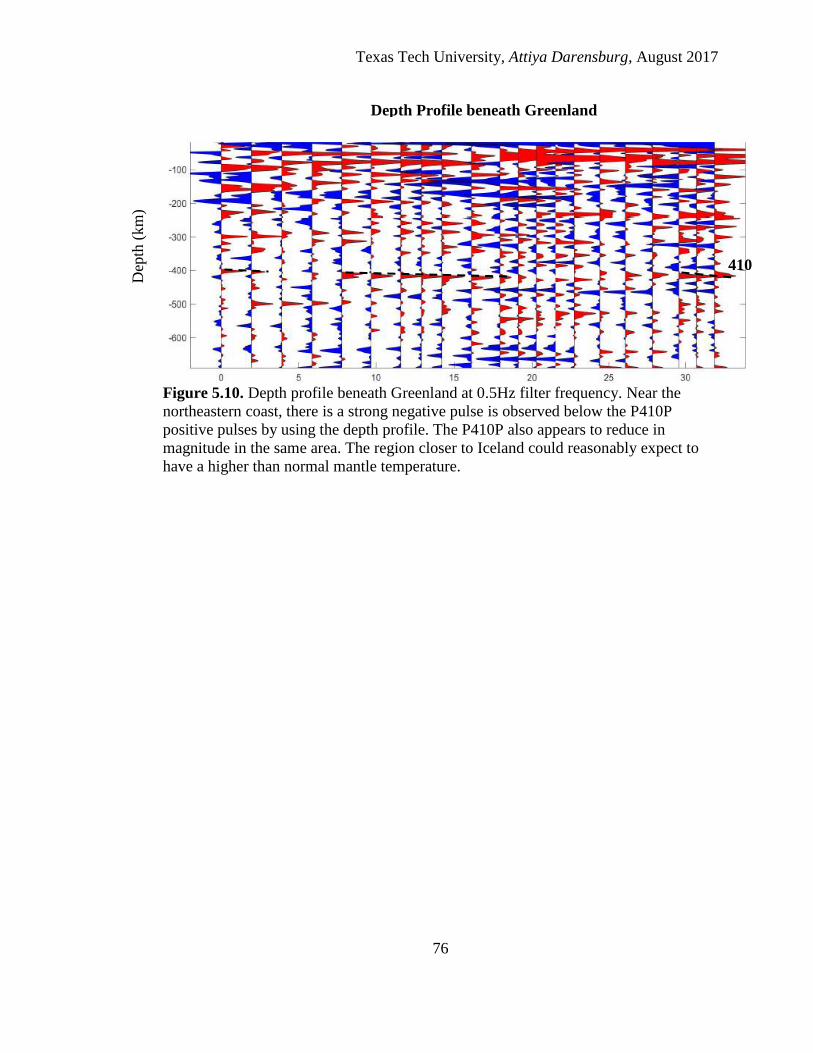
Texas Tech University, Attiya Darensburg, August 2017
76
Figure 5.10. Depth profile beneath Greenland at 0.5Hz filter frequency. Near the
northeastern coast, there is a strong negative pulse is observed below the P410P
positive pulses by using the depth profile. The P410P also appears to reduce in
magnitude in the same area. The region closer to Iceland could reasonably expect to
have a higher than normal mantle temperature.
Depth Profile beneath Greenland
Dep
th (
km
)
410

Texas Tech University, Attiya Darensburg, August 2017
77
CHAPTER VI
CONCLUSION
The 410 km discontinuity cannot be described as a simple exothermic reaction.
We have found some unexpected and complex variations in the depth and amplitude
of the 410 with respet to the proximity of the discontinuity to various styles of tectonic
activity around the world. We have seen the hypothosized transistional boundary
between α-olivine and wadsleyite to occur at unexpected depths to the 410 and P410P
amplitudes relative to thermal anomalies (inferred from maps of Vs). For instance, the
southern tip of the Kamchatka pennisula has P410P amplitudes that are higher than
expected, even though the 410 appears to be shallow. Otherwise, large and sharp
P410P reflections were observed in most areas where the 410 was deep. Higher P410P
amplitudes with narrow pulse widths are expected when the precursor P wave
encounters a narrow velocity gradient between α-olivine and β-olivine/wadsleyite,
where the narrowest velocity gradient yielded the largest and sharpest P410P
amplitudes. As previously mentioned in the discussion section, a deep 410 and a
narrow depth range for the phase change to occur are expected in warmer mantle
environments. A narrow depth range for the phase change should result in a narrower
P410P with a larger amplitude. Large P410P amplitudes were mapped beneath areas
where warm mantle environments are observed like Hawaii, Lake Baikal, NE China,
Iceland, and Alaska.
While most of our results agree with the results from previous studies
conducted in various regions of Earth. While the warm mantle beneath Hawaii and
Iceland are caused by the presence of a hotspot, the source of upper mantle thermal

Texas Tech University, Attiya Darensburg, August 2017
78
anomalies in other regions like Lake Baikal and NE China are poorly understood. For
instance, we found that the mantle is abnormally warm beneath China based on the
depth estimates of the 410, but other studies found the mantle to be cooler beneath
China. We have proposed that despite the presence of a cooler subducting slab
penetrating the upper mantle, the 410 could be warmer due to partial melt caused by
the dehydration of the Philippine plate. Another proposed cause for a warm mantle at
the 410 was the presence of a localized convection cell driven by chemical
replenishment in the peridotite depleted mantle through mélange accumulation at the
base of the TZ due to slab buckling or stagnation (see Ringwood, 1991). Another
possible cause for P410P depth and amplitude variations could be due to a chemically
heterogeneous upper mantle, where the mantle may not be pyrolytic in composition
everywhere (Zindler et al., 1984). If the mantle is indeed warmer at the 410, but cooler
at the 660 beneath China, then it would be reasonable to propose that the transition
between olivine and wadsleyite is more than a simple exothermic reaction as the
inclusion of other chemical compounds complicates the velocity gradient pattern of
this boundary even more. The mantle beneath Lake Baikal is another area where there
is much debate as to the behavior of the mantle beneath this rift zone. Some propose
that the Baikal rift zone is passive (Nilsen and Thybo, 2009) while others believe they
have found proof that it is indeed active where the rift is possibly driven by local
mantle convection (Gao et al., 2003 and Zorin et al., 2003). Our study found the 410 to
be deeper than expected beneath Lake Baikal, which supports the hypothesis that the
Baikal rift is active with a convection cell beneath it.

Texas Tech University, Attiya Darensburg, August 2017
79
Suggestions for future studies
Produce PP and SS precursor maps using 3D velocity modeling
Consider the possibility of iron partitioning in the upper mantle and how it
affects various discontinuities within the upper mantle
Note differences between the region;al depth trends of the 410, 520 and 660,
do they follow the tradition exothermic/endothermic reaction behavior or is the
velocity gradient more complex
Consider a test using a piclogitic mantle model in areas were anomalies occur
Test the velocity gradient of the 410, 520, and 660 on a global scale with a
wider range of frequencies to find the cleanest response without too much
interference from local anomalies

Texas Tech University, Attiya Darensburg, August 2017
80
WORKS CITED
A. E. Ringwood. Composition and Petrology of the Earth’s Mantle. McGraw-Hill,
New York. 1975.
A. E. Ringwood. Phase transformations and their bearing on the constitution and
dynamics of the mantle. Geochimica et Cosmochimica Acta, vol. 55, pages 2083 –
2110. 1991.
Ainiwaer, Ailiyasi. “Synthetic study in amplitude and frequency content of the P410P
phases from common upper mantle discontinuity.” M.S. Thesis, Texas Tech
University, Lubbock, TX, 2014
Akaogi et al. Olivine-Modified Spinel-Spinel Transitions in the System Mg2SiO4 –
Fe2SiO4: Calorimetric Measurements, Thermochemical Calculation, and Geophysical
Application. Journal of Geophysical Research, vol. 94, pages 15671 – 15685.
November 1989.
Anderson and Bass. Transition region of the Earth’s Upper Mantle. Nature, vol. 320,
pages 321 – 328. March 1986.
Artemieva and Thybo. Deep Norden: Highlights of the lithospheric structure of
Northern Europe, Iceland and Greenland. University of Copenhagen, vol. 31, pages
98 – 106. March 2008.
Arwen Deuss et al. The Nature of the 660-Kilometer Discontinuity in Earth’s Mantle
from Global Seismic Observations of PP Precursors. Science, vol. 311, pages 198 –
201. January 2006.
Arwen Deuss. Global Observations of Mantle Discontinuities Using SS and PP
Precursors. Surv Geophys., vol. 30, pages 301 – 326. May 2009.

Texas Tech University, Attiya Darensburg, August 2017
81
Bassin et al. The current limits of resolution for surface wave tomography in North
America. EOS, Trans. Am. Geophys. Un., vol. 81. 2000.
Bina and Helffrich. Phase transition Clapeyron slopes and transition zone seismic
discontinuity topography. Journal of Geophysical Research, vol. 99, pages 15853 –
15860. August 1994.
Chambers et al. Reflectivity of the 410-km discontinuity from PP and SS precursors.
Journal of Geophysical Research, vol. 110, pages 1 – 13. February 2005.
Chen et al. Effect of water on olivine-wadsleyite phase boundary in the (Mg, Fe)2SiO4
system. Geophysical Research Letters, vol. 29. September 2002.
Deschamps et al. Anomalies of temperature and iron in the uppermost mantle inferred
from gravity data and tomographic models. Physics of the Earth and Planetary
Interiors, vol. 129, pages 245 – 264. 2002.
Duan et al. Seismic structure and origin of active intraplate volcanoes in Northeast
Asia. Tectonophysics, vol. 470, pages 257 – 266. January 2009.
Duncan, Gregory. “Processing innovations to improve PP precursor analysis and
increase frequency content of studies in the Mid-Pacific.” M.S. Thesis, Texas Tech
University, Lubbock, TX, 2012
Dziewonski and Anderson, Preliminary reference Earth model, Phys. Earth Planet
Inter., vol. 25, 297 – 356. 1981.
Flanagan and Shearer. Global mapping of topography on transition zone velocity
discontinuities by stacking SS precursors. Journal of Geophysical Research, vol. 103,
pages 2673 – 2692. February 1998.

Texas Tech University, Attiya Darensburg, August 2017
82
Flanagan and Shearer. Topography on the 410-km seismic velocity discontinuity near
subduction zones from stacking of sS, sP, and pP precursors. Journal of Geophysical
Research, vol. 103, pages 21165 – 21182. September 1998.
Flanagan and Shearer. A map of topography on the 410-km discontinuity from PP
precursors. Geophysical Research Letters, vol. 26, pages 549 – 552. March 1999.
Frost and Dolejs. Experimental determination of the effect of H2O on the 410-km
seismic discontinuity. Earth and Planetary Science Letters, vol. 256, pages 182 – 195.
January 2007.
Frost. The Upper Mantle and Transition Zone. Elements, vol. 4, pages 171 – 176. June
2008.
Gao et al. Evidence for small-scale mantle convection in the upper mantle beneath the
Baikal rift zone. Journal of Geophysical Research, vol. 108, pages 1 – 12. April 2003.
Helffrich and Wood. 410-km discontinuity sharpness and the form of the olivine α-β
phase diagram: Resolution of apparent seismic contradictions. Geophysical Journal
International, vol. 126, pages 7 – 12. 1996.
Hirschmann et al. Dehydration melting of nominally anhydrous mantle: The primacy
of partitioning. Physics of the Earth and Planetary Interiors, vol. 176, pages 54 – 68.
April 2009.
HuaiWei et al. Water and partial melting of Earth’s mantle. Science China Earth
Sciences, vol 59, pages 720 – 730. April 2016.
Irifune and Isshiki. Iron partitioning in a pyrolite mantle and the nature of the 410-km
discontinuity. Nature, vol. 392, pages 702 – 704. April 1998.

Texas Tech University, Attiya Darensburg, August 2017
83
Jacobsen et al. Sound velocities of iron-bearing hydrous ringwoodite. Physics of the
Earth and Planetary Interiors, vol. 143 – 144, pages 47 – 56. 2004.
Katsura et al. Adiabatic temperature profile in the mantle. Physics of the Earth and
Planetary Interiors, vol. 183, pages 212 – 218. July 2010.
Kennett, B.L.N. (Ed.), IASPEI 1991 Seismological Tables, Res. Sch. Of Earth Sci.,
Aust. Natl. Univ., Canberra, 1991.
Kind et al. Seismic Images of Crust and Upper Mantle Beneath Tibet: Evidence for
Eurasian Plate Subduction. Science, vol. 298, pages 1219 – 1221. November 2002.
Lawver and Muller. Iceland Hotspot Track. Geology, vol. 22, pages 311 – 314. April
1994.
Lessing et al. Mantle transition zone structure beneath India and Western China from
migration of PP and SS precursors. Geophysical Journal International, vol. 194, pages
396 – 413. January 2014.
Lessing et al. On the difficulties of detecting PP precursors. Geophysical Journal
International, vol. 201, pages 1666 – 1681. 2015.
Nilsen and Thybo. No Moho uplift below the Baikal Rift Zone: Evidence from a
refraction profile across southern Lake Baikal. Journal of Geophysical Research, vol.
114, pages 1 – 22. August 2009.
Nolet et al. Mantle plume tomography. Chemical Geology, vol. 241, pages 248 – 263.
January 2007.
P. M. Shearer. Global mapping of upper mantle reflectors from long-period SS
precursors. Geophysical Journal International, vol. 115, pages 878 – 904. May 1993.
Texas Tech University, Attiya Darensburg, August 2017
84
P. M. Shearer. Transition zone velocity gradients and the 520-km discontinuity.
Journal of Geophysical Research, vol. 101, pages 3053 – 3066. February 1996.
Q. Cao et al. Seismic Imaging of Transition Zone Discontinuities Suggests Hot Mantle
West of Hawaii. Science, vol. 332, pages 1068 – 1071. May 2011.
Ritsema et al. S40RTS: a degree-40 shear-velocity model for the mantle from new
Rayleigh wave dispersion, teleseismic travel time and normal-mode splitting function
measurements. Geophysical Journal International, vol. 184, pages 1223 – 1236. 2011.
Rogers III, Kenneth De Witt. “Investigation of the upper mantle beneath the Hawaiian
Island chain using PP precursors.” M.S. Thesis, Texas Tech University, Lubbock, TX,
2013
Rost and Thomas. Array seismology: methods and applications. Rev. Geophys., vol.
40. 2002.
Rost and Weber. The upper mantle transition zone discontinuities in the Pacific as
determined by short-period array data. Earth Planet. Sci. Lett., vol. 204, pages 347 –
361. 2002.
Schafer et al. Depth variations of the 410 and 520 km-discontinuities beneath Asia and
the Pacific from PP precursors. Geophysical Research Letters, vol. 36. June 2009.
Schmerr and Thomas. Subducted lithosphere beneath the Kuriles from migration of
PP precursors. Earth Planetary Science Letters, vol. 311, pages 101 – 111. 2011.
Shearer and Masters. Global mapping of topography on the 660-km discontinuity.
Nature, vol. 355, pages 791 – 795. February 1992.

Texas Tech University, Attiya Darensburg, August 2017
85
Shearer et al. Experiments in migration processing of SS precursor data to image
upper mantle discontinuity structure. Journal of Geophysical Research, vol. 104,
pages 7229 – 7242. April 1999.
Song et al. P-wave velocity structure under the Changbaishan volcanic region, NE
China, from wide-angle reflection and refraction data. Tectonophysics, vol. 433,
pages 127 – 139. February 2007.
Stixrude. Structure and sharpness of phase transitions mantle discontinuities. J.
Geophys. Res., vol. 102, pages 14835 – 14852. 1997.
Suetsugu et al. Depths of the 410-km and 660-km discontinuities in and around the
stagnant slab beneath the Philippine Sea: Is water stored in the stagnant slab?
Physics of the Earth and Planetary Interiors, vol. 183, pages 270 – 279. September
2010.
Thomas and Billen. Upper mantle structure along a profile in the southwest Pacific.
Geophysical Journal International, vol. 176, pages 113 – 125. 2009.
van der Meijde et al. Seismic evidence for water deep in the Earth’s upper mantle.
Science, vol. 300, pages 1556 – 1558. 2003.
Vidale and Benz. Upper-mantle seismic discontinuities and the thermal structure of
subduction zones. Nature, vol. 356, pages 678 – 683. 1992.
Vink. A hotspot model for Iceland and the Voring Plateau. Journal of Geophysical
Research, vol. 89, pages 9949 – 9959. 1984.
Wood. The effect of water on the 410-kilometer seismic discontinuity. Science, vol.
268, pages 74 – 76. 1995.

Texas Tech University, Attiya Darensburg, August 2017
86
Xueqing Li and Xiaohui Yuan. Receiver functions in northeast China – implications
for slab penetration into the lower mantle in northwest Pacific subduction zone. Earth
and Planetary Science Letters, vol. 216, pages 679 – 691. September 2003.
Yinshuang et al. The crust and upper mantle discontinuity structure beneath Alaska
inferred from receiver functions. Physics of the Earth and Planetary Interiors, vol. 150,
pages 339 – 350. January 2005.
Yusa and Inoue. Compressibility of hydrous wadsleyite (β-phase) in Mg2SiO4 by high
pressure x-ray diffraction. Geophysical Research Letters, vol. 24, pages 1831 – 1834.
1997.
Zhao et al. Imaging the subducting slabs and mantle upwelling under the Japan
Islands. Geophysical Journal International, vol. 190, pages 816 – 828. May 2012.
Zindler et al. Isotope and trace element geochemistry of young Pacific seamounts:
implications for the scale of upper mantle heterogeneity. Earth and Planetary Science
Letters, vol 70, pages 175 – 195. June 1984.
Zorin et al. The Baikal rift zone: the effect of mantle plumes on older structure.
Tectonophysics, vol. 371, pages 153 – 173. May 2003.

Texas Tech University, Attiya Darensburg, August 2017
87
APPENDIX A
USER MANUALS
Run_addPPtimes Manual
This program is the macro for the 3D ray tracing. It runs Nathan's program and outputs
the data to be read in the following programming step. It also references nearly all
other programs that are affilitated with the raytracing process. global zz zz=[0 2 4 6 8 10:5:50 60:20:180 190:10:250 270:20:370 380:10:450
470:40:630 650:20:700 ]; %generates a pre-determined list of depths
we're interested in DIRS=dir([drive_letter ':\CUT_PP\' year]) %places us in the correct
directoyy for i=3:length(DIRS) if exist([drive_letter ':\CUT_PP\' year '\' DIRS(i).name
'\Good_files.mat'])~=0 load([drive_letter ':\CUT_PP\' year '\' DIRS(i).name
'\Good_files.mat']) %if Good_files exists in the directory, then we
want to load it
fid2=fopen('PP_raypath.txt','wt'); % seting up command line
for event to station with all raypath info for jmp=1:length(Good_files) % this loop sets up a bunch of
files to run nathan's program for midpoints RFNT=Good_files(jmp).name; RFNT=[drive_letter RFNT(2:end)]; dashes=find(RFNT=='/'); %correcting the slash issue that
arrises when QCing is done on a Mac RFNT(dashes)='\'; RFN(jmp).name=RFNT; load(RFN(jmp).name) mpname(jmp).name=set_up_midpoints(data,jmp); clear data fprintf(fid2,['-raytrace LLNL-G3D-JPS.e3d.binary '
mpname(jmp).name ' -p']); %initiates the 3D raytracing program. The
binary file must be in the path. fprintf(fid2,['\n']); end fprintf(fid2,['quit']); fclose(fid2); system('java -jar LLNL-Earth3D.5.3.jar < PP_raypath.txt') %
runs nathan's program for midpoints. The system command is needed
because it is written in java.
for jmp=1:length(Good_files) % reads files and gets midpoints if exist([mpname(jmp).name '.0.ascii.path']) > 0.5
[mlat(jmp),mlon(jmp),mz(jmp)]=get_midpoints(mpname(jmp).name); %calls
the get_midpoints program end end

Texas Tech University, Attiya Darensburg, August 2017
88
fid5=fopen('PP_time_midpoint_to_station.txt','wt');% doing
the raytracing for each depth of the midpoint - here we are opening
the times for the first leg of the PP wave for jmp=1:length(Good_files) load(RFN(jmp).name)
[zzname(jmp).name,]=make_ZZ_vs_TT(data,mlon(jmp),mlat(jmp),mz(jmp),jm
p); %makes zzname file, times to the depths fprintf(fid5,['-raytrace LLNL-G3D-JPS.e3d.binary '
zzname(jmp).name]); %running Nathan's program fprintf(fid5,['\n']); end fprintf(fid5,['quit']); fclose(fid5) % done setting up command to trace from
midpoint to station P wave system('java -jar LLNL-Earth3D.5.3.jar <
PP_time_midpoint_to_station.txt') % initiating Nathan's program to
trace from midpoint to station
for jmp=1:length(Good_files) hi=RFN(jmp).name if exist([zzname(jmp).name '.TT']) > 0.5 % if the zzname
file exists, then load it to read data load(RFN(jmp).name) [ZZ,dtt]=get_ZZ_vs_TT(zzname(jmp).name,mz(jmp)); %
run the program to make the list of ZZ vs dtt data(3).zz=ZZ; % want the data in the 3rd channel data(3).dtt=dtt; D=data(3); clear data data=D; clear D dashes=find(RFN(jmp).name=='\'); RFN_out=[RFN(jmp).name(1:dashes(1)) 'CUT_PP_TT'
RFN(jmp).name(dashes(2):end)]; RFN_out(1)=outdrive; dashes=find(RFN_out=='\'); % fixes the slash issue on
Macs mkdir(RFN_out(1:dashes(end))) % makes a new directory
for the new data save(RFN_out,'data') %saves it end end end % each time this function is ran, the used data needs to be
deleted so that it isn't overwritten !del mid_pt*txt* !del Z_vs_t*txt* !del *txt !del *TT !del *TT end end

Texas Tech University, Attiya Darensburg, August 2017
89
PPnSSbeamer Manual
In order to run this program you must open run_PPnSSbeamer to access enter the
input variables, ‘PP’ for phase is the first input, the second input is the drive letter you
want the program to write all of your outputs onto.
The time at which the PP precursor arrives is ideally around 200 seconds after the
initial impulse, so time_total or the total length of the time window for PP waves is set
at 289 seconds
D_dirs(i).name is used to categorize the highsn, others and lowsn folders as i=1,2,3
respectively for filtering data and obtaining amplitudes for convolution and stacking
later on
Empty matricies for Df (filtered deoceaned source functions) and MIDPT(midpoint
information) is created for future storage
If any of the event folders exists (highsn, lowsn, or others) the program changes the
working directory form the home directory(home1, the home directory always starts
from the year of interest) to the event folder with highsn, lowsn or others.
After the program locates all BHZ networks, it enters the “for” loop processing one
file for the event at a time. If the depth of the earthquake is greater than 60 km, it is
classified as an event that is too deep, the “for” loop ends and that event is skipped,
moving on to the next.
The variable iFs was set to zero before the start of the “for” loop. This is a counter,
keeping track of the number of events that are shallow enough to be used for the rest
of the data processing procedure.
The variable dt is assigned to store the value of the current sample rate of the data file
The variable Dt is assigned to store amplitude values for the data file
Using GFILT_2015: Dt is high pass filtered at 0.02 Hz using the raw data, the now
filtered data file is filtered again, but instead it is low pass filtered at 0.5Hz. These two
filtering steps effective apply a taper to the upper and lower limits of the raw data
The filtered data is interpolated to a sample rate of 0.05s/sample. The impulses for the
new filtered data is saved as variable Dft
The newly interpolated data is low pass filtered again at 0.5 Hz
Amplitudes/impulses are saved as within each file as data.data
The sample rate is saved within each file as data.dt
Variables w1 and w2 are the time windows for the PP precursor wave (10 s prior and
30 s after)
Impulses from the filtered waveform is saved as variable Df, noise from the Dft
version is minimized via standard deviation of the Dft wave, the same applies for Do,
except the Dt wave is used
Event names, locations and station locations are all saved with the “data” array as
NAME, EVENT and STA respectively
Once the information for the data file is saved within itself as the structured array
“data”, the directory is changed to the “Nathan_7_22_2016_Beamform” folder (this
enables raytracing and beamforming to run concurrently without overwriting midpoint
data being created in via the 3D raytracing program “run_addPPtimes”)

Texas Tech University, Attiya Darensburg, August 2017
90
Midpoint location, depth and elevation relative to sea level are all obtained via
“run_trace_PPmidptWB” with event and station information used as input variables.
EVENT is transposed in order to store the information in rows instead of columns
Midpoint data is saved within the empty vector, MIDPT, created at the beginning of
the program
All waveforms with dry or wet bouncepoints are convolved with themselves. The
maximum amplitudes are stored as variable “Afm”. Dry bouncepoints are defined by a
waveform with a midpoint beneath a landform. Wet bouncepoints are defined by
waveforms with midpoints in the middle of the ocean *note: the flipud command is
flipping the impulses/amplitudes for the waveform left/right instead of up/down due
to the impulse data being stored in a row instead of a column
Elevation of the bouncepoints for each data set are sorted from shallowest to deepest
elevation. All data information within each file is saved within itself as the structured
array “data(1)”
All wet bouncepoints are found via traced raypaths with the use of the
PP_RM_OCEAN program. The raw and filtered source functions are saved as Do_S
and Df_S respectively
Maximum amplitudes are saved as MAX_AMPs for events with highsn and others
Data is stacked through different degree bin sizes and saved as channels 11, 12, 13, 14,
15 and 16 (0.5°,1°, 2°, 4°, 8° and 16° respectively). These channels are reserved for
the raw data
Channels 35 and 36 are deoceaned source functions
AMPjunk is reserved for amplitudes and IMA is reserved at the location for each
impulse
BEAM180ALL.mat file is saved within every event folder
All deoceaned filtered data is stacked within 180° bins and stored as channel 40
(GCarc)
BEAM180ALL and BEAM180DRY are saved as mat files in every event folder
All event information is saved as the structured array “EVENTS_INFO”

Texas Tech University, Attiya Darensburg, August 2017
91
APPENDIX B
QC GUIDE
Attiya Darensburg
QC guide
For the PP data we are focusing on the 410 km discontinuity since it appears the
clearest for the PP phase. In particular, we want to select seismic wave forms where
the greatest impulse happens exactly at or close to 200 seconds (highlighted by a
vertical red line). Some seismograms can be tricky. If an impulse is observed toward
the beginning of the event 0 seconds or close to this point, it can be assumed that this
is the direct P wave arrival, an entirely separate event that will not interfere with other
impulses that may be observed later on in time for the same event. Some events that
have impulses which do not occur exactly when we would prefer might be acceptable
under certain circumstances, for instance, if there are a low number of wave forms or
seismograms for a particular event, forcing one to be more lenient in regards to which
seismogram should be kept. The following screenshots are examples of events that
should be accept or rejected as well as under which circumstances these decisions may
change.
When you run ALL_PPnSSCLEAN2_2015, the first input is the channel followed by
the phase type (ALL_PPnSSCLEAN2_2015(‘3’,’PP’)). The channel for all PP phases
is channel 3; channel 2 is reserved for SS phases.
The following screenshots are examples of seismograms that should be kept:

Texas Tech University, Attiya Darensburg, August 2017
92

Texas Tech University, Attiya Darensburg, August 2017
93

Texas Tech University, Attiya Darensburg, August 2017
94
The greatest amplitudes for these 3 seismograms appears to occur around 210 seconds,
but more importantly, the initial drastic increase in amplitude is observed exactly at
200 seconds
The next series of screenshots are examples of seismograms that should fall in the “in
between” category of whether they should be kept or rejected. This decision typically
depends on how many seismograms are left in a given event and how many have
already been accepted:
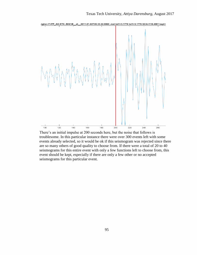
Texas Tech University, Attiya Darensburg, August 2017
95
There’s an initial impulse at 200 seconds here, but the noise that follows is
troublesome. In this particular instance there were over 300 events left with some
events already selected, so it would be ok if this seismogram was rejected since there
are so many others of good quality to choose from. If there were a total of 20 to 40
seismograms for this entire event with only a few functions left to choose from, this
event should be kept, especially if there are only a few other or no accepted
seismograms for this particular event.

Texas Tech University, Attiya Darensburg, August 2017
96
The largest impulse is observed at 220 seconds, but this should still be kept as the
largest amplitude does not arrive too late.

Texas Tech University, Attiya Darensburg, August 2017
97
Here’s another example of a seismogram that should be accepted only if your options
are limited. Notice how the largest observed impulse is after 260 seconds, long after
the PP arrival, but the initial impulse is around 210 seconds. The second arrival is
possibly far enough away to not interfere with the P410P arrival.

Texas Tech University, Attiya Darensburg, August 2017
98
This impulse arrives a little early, but once again, it would be a good seismogram to
keep if your options are limited. For seismograms in the “others” category it would be
a good idea to keep this seismogram since it is not likely that you will find nice and
clean signals as often as you would with “highsn” files.
*One thing to keep in mind is that the reason why we QC is to find waveforms that
can be successfully cross correlated with high quality waveforms. It is better to error
on the side of caution and accept “good enough” seismograms when you don’t have a
lot of options. When these individual selected events are processed through the cross
correlation program, the seismograms that could not cross correlate with a value equal
to or greater than 0.6 or 0.7 are rejected anyway.
The following screenshots are examples of bad seismograms that should be rejected:

Texas Tech University, Attiya Darensburg, August 2017
99
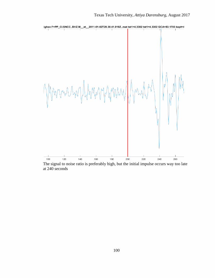
Texas Tech University, Attiya Darensburg, August 2017
100
The signal to noise ratio is preferably high, but the initial impulse occurs way too late
at 240 seconds

Texas Tech University, Attiya Darensburg, August 2017
101
Noisy

Texas Tech University, Attiya Darensburg, August 2017
102

Texas Tech University, Attiya Darensburg, August 2017
103

Texas Tech University, Attiya Darensburg, August 2017
104