2016 > Environmental studies > Air - admin.ch · 2016 > Environmental studies > Air > Critical...
80
> Air > Environmental studies 2016 > Critical Loads of Nitrogen and their Exceedances Swiss contribution to the effects-oriented work under the Convention on Long-range Transboundary Air Pollution (UNECE)
Transcript of 2016 > Environmental studies > Air - admin.ch · 2016 > Environmental studies > Air > Critical...
> Air> Environmental studies2016
> Critical Loads of Nitrogen and their Exceedances
Swiss contribution to the effects-oriented work under the Convention on Long-range Transboundary Air Pollution (UNECE)

> Air> Environmental studies
Published by the Federal Office for the Environment FOENBern, 2016
> Critical Loads of Nitrogen and their Exceedances
Swiss contribution to the effects-oriented work under the Convention on Long-range Transboundary Air Pollution (UNECE)

Publisher Federal Office for the Environment (FOEN) The FOEN is an office of the Federal Department of Environment, Transport, Energy and Communications (DETEC).
Authors Beat Rihm, Meteotest, Bern Beat Achermann, FOEN
In-house consultant Reto Meier, Air Pollution Control and Chemicals Division
Suggested form of citation Rihm B., Achermann B. 2016: Critical Loads of Nitrogen and their Exceedances. Swiss contribution to the effects-oriented work under the Convention on Long-range Transboundary Air Pollution (UNECE). Federal Office for the Environment, Bern. Environmental studies no. 1642: 78 p.
Design Stefanie Studer, 5444 Künten
Cover picture FOEN
Link to PDF file www.bafu.admin.ch/uw-1642-e It is not possible to order a printed version.
© FOEN 2016
> Table of contents 3
> Table of contents
Abstracts 5
Foreword 7
Summary 8
1 Background and Aims 11
1.1 The Critical Loads and Levels approach developed under the UNECE Convention on Long-range Transboundary Air Pollution 11
1.2 Mapping Critical Loads and Levels in Switzerland 14
2 Methods to Derive Critical Loads of Nutrient Nitrogen 16
2.1 Adverse Effects of Exposure to Atmospheric Nitrogen Compounds 16
2.1.1 Direct Toxicity of Nitrogen Gases 17
2.1.2 Eutrophication of (semi-)natural Ecosystems 17
2.1.3 Soil Acidification 18
2.1.4 Increased Susceptibility to Secondary Stress Factors 18
2.2 Empirical Critical Loads of Nitrogen 18
2.2.1 The Empirical Method 18
2.2.2 Derivation of Country-specific Empirical Critical Loads 20
2.2.3 Mapping Empirical Critical Loads for Ecosystems in Switzerland 23
2.3 The Simple Mass Balance Method (SMB) 29
2.3.1 The Calculation Method 29
2.3.2 Quantification of the Input Parameters 31
3 Mapping Nitrogen Deposition 36
3.1 Modelling Approach 36
3.2 Wet Deposition 38
3.3 Dry Deposition of Gases 40
3.4 Dry Deposition of Aerosols 43
3.5 Mapping Ammonia 45
3.5.1 Emissions of Ammonia 45
3.5.2 Ammonia Concentration 50
3.5.3 Validation of the Ammonia Maps 52
3.6 Mapping Depositions 1990–2010 54
4 Results 55
4.1 Critical Loads of Nitrogen 55
4.2 Deposition of Nitrogen 58
4.3 Exceedances of Critical Loads of Nitrogen 60
4.4 Reliability of the Results 64
5 Conclusions 66
Annex 68
Ammonia Dispersion Function 68
Bibliography 69 Glossary 75 Abbreviations, figures and tables 76


> Abstracts 5
> Abstracts
Critical loads are defined as those air pollutant depositions below which harmful
effects on specified sensitive receptors of the environment do not occur according to
present scientific knowledge. They are an established element for developing effects-
based approaches under the UNECE Convention on Long-range Transboundary Air
Pollution. Critical loads of nitrogen were determined and mapped for forests and for
(semi-)natural ecosystems in Switzerland by applying two methods proposed by the
UNECE: the simple mass balance (SMB) and the empirical method. Total nitrogen
deposition was modelled with high spatial resolution for the time period 1990–2010. In
2010, the nitrogen deposition exceeded the critical loads on more than 90% of all forest
sites and on approximately 70% of the (semi-)natural ecosystems.
Keywords:
Critical loads of nitrogen,
(semi-) natural ecosystems,
nitrogen deposition, exceedance
of critical loads, UNECE LRTAP
Convention
Als Critical Loads werden jene Depositionen oder Einträge von Luftschadstoffen
bezeichnet, unterhalb welchen nach dem heutigen Stand des Wissens keine schädlichen
Auswirkungen auf empfindliche Rezeptoren der Umwelt auftreten. Im Rahmen der
Konvention über weiträumige grenzüberschreitende Luftverunreinigung (UNECE) sind
die Critical Loads wichtige Zielgrössen zur Entwicklung von wirkungsorientierten
Luftreinhaltestrategien. Critical Loads für Stickstoff wurden in der Schweiz für Wälder
und (halb)natürliche Ökosysteme mit zwei von der UNECE vorgeschlagenen Metho-
den bestimmt und kartiert: die Massenbilanzmethode (SMB) und die empirische Me-
thode. Die Deposition von stickstoffhaltigen Luftschadstoffen wurde für den Zeitraum
1990–2010 in einer hohen räumlichen Auflösung modelliert. Im Jahr 2010 wurden die
Critical Loads für Stickstoff bei mehr als 90% der Waldökosysteme und bei rund 70%
der (halb)natürlichen Ökosysteme überschritten.
Stichwörter:
Critical Loads für Stickstoff,
(halb)natürliche Ökosysteme,
Stickstoffdeposition,
Überschreitung der Critical
Loads, UNECE LRTAP
Convention
La notion des charges critiques représente une estimation quantitative des dépôts de
polluants atmosphériques au-dessous desquels, selon les connaissances actuelles, il n’y
a pas d’effets nocifs pour des milieux sensibles de l’environnement. L’approche basée
sur les charges critiques est un élément essentiel de la Convention sur la pollution
transfrontière à longue distance (CEE ONU) pour le développement de stratégies de
lutte contre la pollution de l’air basées sur les effets. En Suisse, les charges critiques
pour l’azote ont été déterminées et cartographiées pour les forêts et les écosystèmes
(semi-)naturels en appliquant deux méthodes recommandées par la CEE ONU: le
«bilan à l’équilibre» (SMB) et une méthode dite empirique. Les dépôts de composés
azotés atmosphériques ont été modélisés pour la période 1990–2010 avec une résolu-
tion spatiale élevée. En 2010, ces dépôts dépassaient les charges critiques pour l’azote
sur plus que 90% des sites forestiers et dans environ 70% des écosystèmes (semi-)
naturels.
Mots-clés:
Charges critiques pour l’azote,
écosystèmes (semi-)naturels,
dépôts de composés azotés,
dépassement de charges
critiques, UNECE LRTAP
Convention

Critical Loads of Nitrogen and their Exceedances FOEN 2016 6
La nozione dei carichi critici rappresenta una stima quantitativa dei depositi di inqui-
nanti atmosferici al di sotto dei quali, secondo le conoscenze attuali, non ci sono effetti
nocivi per i ricettori ambientali particolarmente sensibili. L’approccio basato sui carichi
critici è un elemento essenziale della Convenzione sull’inquinamento atmosferico
transfrontaliero a grande distanza (CEE ONU) per lo sviluppo di strategie di lotta con-
tro l’inquinamento dell’aria basata sugli effetti. In Svizzera, i carichi critici per l’azoto
sono stati determinati e mappati per le foreste e gli ecosistemi (semi-)naturali applican-
do due metodi raccomandati dalla CEE ONU: il metodo del “bilancio a l’equilibrio”
(Simple Mass Bilance) e il metodo detto empirico. I depositi di composti azotati atmo-
sferici sono stati modellizzati per il periodo 1990–2010 con una risoluzione spaziale
elevata. Nel 2010, questi depositi oltrepassavano i carichi critici per l’azoto su più di
90% dei siti forestali e nel circa 70% degli ecosistemi (semi-)naturali.
Parole chiave:
Carichi critici per l’azoto,
ecosistemi (semi-)naturali,
depositi di composti azotati,
superamento dei carichi critici,
UNECE LRTAP Convention
> Foreword 7
> Foreword
A critical load is defined as “a quantitative estimate of an exposure to one or more air
pollutants below which significant harmful effects on specified sensitive elements of
the environment do not occur according to present knowledge”. The critical loads
approach was developed under the Convention on Long-range Transboundary Air
Pollution (UNECE LRTAP Convention) and its Working Group on Effects to support
effects-oriented air pollution abatement policies. High atmospheric deposition of
sulphur and nitrogen compounds and their harmful effects on sensitive ecosystems in
terms of acidification and eutrophication were at the origin of substantial scientific
efforts to derive ecosystem-specific critical loads of acidity and critical loads of nutri-
ent nitrogen. To enable the long-term protection of ecosystems, the critical loads
should not be exceeded by atmospheric deposition of sulphur and nitrogen. Many
scientific workshops were held under the Convention since 1988 aiming at setting
critical loads reflecting the most recent scientific knowledge on effects of air pollu-
tants. The UNECE Manual on Methodologies and Criteria for Modelling and Mapping
Critical Loads & Levels and Air Pollution Effects, Risks and Trends summarizes these
scientific findings and gives guidance to Parties to the Convention on how to apply the
critical loads approach. Today, the critical loads and levels approach is an important
element in the structure of the Gothenburg Protocol negotiated under the LRTAP
Convention to abate acidification, eutrophication and ground-level ozone. According to
the objective of this Protocol, the emissions of sulphur, nitrogen oxides, ammonia,
volatile organic compounds and particulate matter shall be reduced to ensure that, in
the long-term and in a step-wise approach, atmospheric depositions or concentrations
do not exceed critical loads of acidity, critical loads of nutrient nitrogen, critical levels
of ozone, critical levels of particulate matter, critical levels of ammonia and acceptable
levels of air pollutants to protect materials.
Swiss scientists and experts have actively participated in the further development of the
critical loads and levels approach under the LRTAP Convention. The report presented
here focuses on the critical loads of nutrient nitrogen and their exceedances by elevated
atmospheric deposition of nitrogen compounds on sensitive (semi-)natural ecosystems.
It mainly reflects the scientific knowledge resulting from the workshops on critical
loads of nitrogen held under the auspices of the Convention in Lökeberg (1992), in
Berne (2002) and in Noordwijkerhout (2010), and it considers as well results from
experimental work in natural ecosystems and from gradient studies carried out by
scientists in Switzerland. The report is an update of the report on critical loads of
nitrogen published by the Federal Office in 1996 (Environmental Series No. 275).
We are convinced that the ongoing work on critical loads and levels has the potential to
contribute to increasing the quality and ambition level of future international agree-
ments on the control of air pollutant emissions and also to the further development of
national and regional air pollution control policies on the basis of effects-oriented
assessments of impacts of air pollutants on sensitive ecosystems.
Martin Schiess
Head of the Air Pollution Control and Chemicals Division
Federal Office for the Environment (FOEN)
Critical Loads of Nitrogen and their Exceedances FOEN 2016 8
> Summary
The negotiations on air pollution abatement strategies under the UNECE Convention
on Long-range Transboundary Air Pollution are based on an effects-based critical
levels / loads approach. Critical levels / loads are defined as those air pollutant concen-
trations / depositions below which harmful effects on specified sensitive receptors of
the environment do not occur according to present scientific knowledge.
Under the Convention, the International Cooperative Programme (ICP) on “Modelling
and Mapping Critical Levels and Loads and Air Pollution Effects, Risks and Trends”
aims at developing scientific methods to compute and map the ecosystem sensitivities
to air pollutants in the ECE region. A regularly updated Manual on Methodologies and
Criteria for Mapping Critical Loads and Levels gives guidance to the Parties to the
Convention to apply the most appropriate methods to assess the exposure of the eco-
systems on their territory and the associated risks. At present, more than 20 countries
are taking part in the ICP. Most of the countries supply national data and maps to the
Coordination Centre for Effects (CCE), where the European maps are compiled and
overall risk assessments are carried out.
For Switzerland, critical loads of nitrogen were computed using two methods proposed
by the ICP: (1) the simple (steady state) mass balance method (SMB) for forests; and
(2) the empirical method for natural and semi-natural ecosystems such as raised bogs,
fens, dry or species-rich grassland, mountain hay meadows, (sub)alpine grassland,
alpine scrub habitats and alpine lakes.
The SMB balances the atmospheric depositions against the natural long-term processes
that permanently immobilise nitrogen or remove it from the (eco-)system. The SMB
was applied on a 1 x 1 km² grid, with 10 632 points representing productive forests, i.e.
sites where harvesting is possible.
The empirical method is based on results from scientific field studies with nitrogen
addition experiments, from field observation studies along nitrogen deposition gradi-
ents, from mesocosm studies, but also on expert judgement. The result is a list of
sensitive ecosystem types in Europe with corresponding ranges of approved critical
load values. Swiss critical load maps were produced by assigning appropriate values
from that list to the national inventories of ecosystems worthy to be protected (raised
bogs, fens, dry grasslands (TWW), various ecosystems listed in the Swiss Atlas of
Vegetation Types Worthy of Protection, data set of the Swiss Biodiversity Monitoring).
For the use of the maps under the Convention, the maps were aggregated to a 1 x 1 km²
raster with a total area of 18 584 km² containing sensitive ecosystems.
Nitrogen deposition in 1990, 2000 and 2010 was mapped using a pragmatic approach
that combines emission inventories, statistical dispersion models, monitoring data,
spatial interpolation methods and inferential deposition models. The following com-
pounds were considered: wet and dry deposition of nitrate (NO3-) and ammonium
> Summary 9
(NH4+) as well as gaseous deposition of ammonia (NH3), nitrogen dioxide (NO2) and
nitric acid (HNO3).
The resulting critical loads of nitrogen show a variation of 4 to 25 kg N ha-1 a-1, de-
pending on ecosystem type, soil type, altitude and other ecosystem properties. Nitrogen
depositions in 2010 were in the range of 2 to 65 kg N ha-1 a-1, the highest values occur-
ring in the lowlands. The total deposition in Switzerland amounts to 67 kt N a-1 (44 kt
N a-1 of reduced nitrogen plus 23 kt N a-1 of oxidised nitrogen). From 1990 to 2010 the
total deposition of nitrogen compounds decreased by 23%.
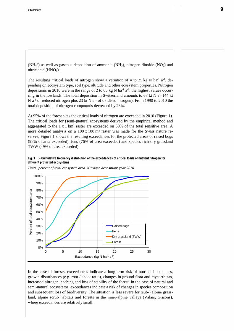
At 95% of the forest sites the critical loads of nitrogen are exceeded in 2010 (Figure 1).
The critical loads for (semi-)natural ecosystems derived by the empirical method and
aggregated to the 1 x 1 km² raster are exceeded on 69% of the total sensitive area. A
more detailed analysis on a 100 x 100 m² raster was made for the Swiss nature re-
serves; Figure 1 shows the resulting exceedances for the protected areas of raised bogs
(98% of area exceeded), fens (76% of area exceeded) and species rich dry grassland
TWW (49% of area exceeded).
Fig. 1 > Cumulative frequency distribution of the exceedances of critical loads of nutrient nitrogen for different protected ecosystems
Units: percent of total ecosystem area. Nitrogen deposition: year 2010.
In the case of forests, exceedances indicate a long-term risk of nutrient imbalances,
growth disturbances (e.g. root / shoot ratio), changes in ground flora and mycorrhizas,
increased nitrogen leaching and loss of stability of the forest. In the case of natural and
semi-natural ecosystems, exceedances indicate a risk of changes in species composition
and subsequent loss of biodiversity. The situation is less severe for (sub-) alpine grass-
land, alpine scrub habitats and forests in the inner-alpine valleys (Valais, Grisons),
where exceedances are relatively small.
0%
10%
20%
30%
40%
50%
60%
70%
80%
90%
100%
0 5 10 15 20 25 30
Pe
rcen
t o
f to
tal e
co
syste
m a
rea
Exceedance (kg N ha-1 a-1)
Raised bogs
Fens
Dry grassland (TWW)
Forest
Critical Loads of Nitrogen and their Exceedances FOEN 2016 10
An important step to improve this situation will be made by achieving the 2020 emis-
sion reduction targets of the Gothenburg Protocol as revised in 2012. Further emission
reductions under this international agreement beyond 2020 are possible and would
result in substantial benefits for the environment.
1 > Background and Aims 11
1 > Background and Aims - - - - - - - - - - - - - - - - - - - - - - - - - - - - - - - - - - - - - - - - - - - - - - - - - - - - - - - - - - - - - - - - - - - - - - - - - - - - - - - - - - - - - - - - - - - - - - - - - - - - - - - - - - - - - - -
1.1 The Critical Loads and Levels approach developed under the UNECE Convention on Long-range Transboundary Air Pollution
Since 1979 the Convention on Long-range Transboundary Air Pollution (LRTAP
Convention, UNECE1) has addressed several environmental problems of the ECE
region through scientific collaboration and policy negotiation. A good scientific under-
standing of the harmful effects of air pollution was recognised as a prerequisite for
reaching political agreement on targeted pollution control. To develop the necessary
international cooperation in the research on and the monitoring of pollutant effects, the
Working Group on Effects (WGE) along with Task Forces and International Coopera-
tive Programmes (ICPs) were established under the Convention. The EMEP2 pro-
gramme provides support to the Convention in the field of atmospheric transport
modelling of pollutants.
At the sixth session of the Executive Body for the Convention in 1988, a Task Force on
Mapping Critical Levels / Loads was established, with the aim of developing the
mapping approaches needed to show the extent of the sensitivity of ecosystems to air
pollution and the exceedances of critical levels / loads in the ECE region. Later the
Task Force was renamed to ‘ICP Modelling and Mapping of Critical Loads & Levels
and Air Pollution Effects, Risks and Trends’ (ICP Modelling & Mapping or ICP
M&M3).
The basic idea of the critical load concept is to balance the depositions which an eco-
system is exposed to with the capacity of this ecosystem to buffer the input (e.g. the
acidity input buffered by the weathering rate), to remove it from the system (e.g.
nitrogen by plant uptake and harvest) or to immobilize it in the long-term without
harmful effects within or outside the system. Accordingly, a critical load is defined as
“a quantitative estimate of an exposure to one or more pollutants below which signifi-
cant harmful effects on specified sensitive elements of the environment do not occur
according to present knowledge” (Nilsson & Grennfelt 1988, UNECE 2012). In the
case of eutrophying effects of nitrogen the term “exposure” relates to the sum of the
depositions of reduced nitrogen compounds (NHx) and oxidised nitrogen compounds
(NOy). “Sensitive elements of the environment” can be whole ecosystems or part of
them by addressing ecosystem development processes, structure and function (UNECE
2016, Chapter V.1).
The work programme under the ICP Modelling & Mapping includes the production of
maps of critical loads, critical levels and their exceedances as a basis for developing
effects-based abatement strategies for transboundary air pollutants. Several scientific
1 www.unece.org/env/lrtap/welcome.html 2 www.emep.int 3 www.icpmapping.org
Definition of the critical load
Critical Loads of Nitrogen and their Exceedances FOEN 2016 12
workshops were held under the auspices of the UNECE to define critical levels and
critical loads for sensitive receptors of the environment and to discuss the methods for
mapping them. Critical levels have been defined for the direct effects of ambient
concentrations of SO2, NOx (NO and NO2), NH3 and O3 on different vegetation types
and on materials. Methods for the computation of critical loads of acidity (sulphur and
nitrogen), of nutrient nitrogen with respect to eutrophication and of heavy metals have
been proposed for aquatic and terrestrial ecosystems.
With respect to critical loads of nutrient (eutrophying) nitrogen the following scientific
workshops and meetings were held under the Convention:
> Workshop on critical loads for sulphur and nitrogen in Skokloster, Sweden, 1988
(Nilsson & Grennfelt 1988);
> Workshop on critical loads for nitrogen in Lökeberg, Sweden, 1992 (Grennfelt &
Thörnelöf 1992);
> WHO workshop on Air Quality Guidelines for Europe, held in Les Diablerets,
Switzerland (WHO/Europe 1995);
> Workshop on critical loads for nitrogen in Grange-over-Sands, United Kingdom,
1994 (Hornung et al. 1995);
> Meeting of the Task Force on Mapping with expert pre-meetings on empirical
critical loads of nitrogen in Geneva, Switzerland, December 1995 (UNECE 1995);
> Expert Workshop on empirical critical loads for nitrogen, Berne, Switzerland, 11–13
November 2002 (Achermann & Bobbink 2003);
> Expert Workshop on review and revision of empirical critical loads and dose-
response relationships, Noordwijkerhout, The Netherlands, 23–25 June 2010 (Bob-
bink & Hettelingh 2011).
Several workshops and meetings of the ICP Modelling & Mapping have led to the
production and repeated revision of a “Manual on Methodologies for Mapping Critical
Levels / Loads and Geographical Areas where they are Exceeded” (UNECE 1993,
1996, 2004 and 2016). The manual supplies a scientific basis and guidelines for gather-
ing, handling and processing data on the basis of which Parties to the Convention are
able to:
> determine and identify sensitive receptors and locations;
> map critical levels and loads on a national scale;
> map areas where air pollutant concentrations or depositions exceed critical levels or
loads.
In order to provide scientific and technical assistance to the Task Force on Modelling
& Mapping and to National Focal Centres (NFCs), a Coordination Centre for Effects
(CCE4) was established at the National Institute for Public Health and the Environment
(RIVM) in Bilthoven, The Netherlands. Since 1990 the CCE organizes annual training
sessions for national mapping experts and for dynamic modellers, where technical
aspects of the modelling and mapping approaches are discussed and coordinated.
4 http://wge-cce.org
Scientific workshops addressing
critical loads of nitrogen
Coordination Centre for Effects

1 > Background and Aims 13
The CCE produces the “best available” integrated European critical levels / loads and
exceedance maps, based primarily upon data supplied by individual countries and by
EMEP. Since 1991, it also publishes technical reports on modelling and mapping
covering topics such as critical loads of sulphur and nitrogen and their exceedances,
dynamic modelling of soil processes, effects on ecosystems and biodiversity (e.g.
Hettelingh et al. 1991, Posch et al. 2012, Slootweg et al. 2015).
In order to ensure the coordination of the national mapping activities, the Parties to the
Convention were invited to establish National Focal Centres (NFCs). The Swiss Na-
tional Focal Centre is located at the Federal Office for the Environment (FOEN).
With regard to critical loads the most important activities under the Convention on
LRTAP can be summarised as follows.
According to the work plan of the Executive Body for the Convention, the first maps to
be produced at the European scale in 1991/1992 were the map on critical loads of
acidity and the map on critical loads of sulphur derived from it. Both maps were suc-
cessfully used as a basis for developing effects-based and cost-optimized sulphur
emission abatement scenarios by the UNECE Task Force on Integrated Assessment
Modelling5. The scenario results have been used by the UNECE Working Group on
Strategies in the negotiation process for the Protocol on the further reduction of sulphur
emissions, which was signed in Oslo, Norway, in June 1994.
A second step under the Convention was the revision of the 1988 Protocol concerning
the Control of Nitrogen Oxides. Critical loads of nitrogen played an important role in
the development of optimized scenarios to control nitrogen compounds with respect to
acidification and eutrophication. First maps with critical loads of nitrogen were pro-
duced by the CCE in 1995 on the basis of national contributions, and, where not avail-
able, by applying the mass balance approach with European default values for forest
sites. These maps were discussed by the Task Force on Mapping and adopted by the
Working Group on Effects in 1995. The Task Force on Integrated Assessment Model-
ling (TFIAM) used the maps for the development of optimized nitrogen abatement
scenarios for the ECE region. These scenarios formed the effect-oriented basis for the
1999 Gothenburg Protocol6 concerning the reduction of emissions of sulphur dioxide
(SO2), nitrogen oxides (NOx), volatile organic compounds (VOCs) and ammonia
(NH3).
The Gothenburg Protocol was amended in 2012 to include particulate matter (PM) and
national emission reduction commitments for SO2, NOx, NH3, VOCs and PM2.5 to be
achieved in 2020. Again, the European critical load database compiled and updated by
the CCE in collaborations with the National Focal Centres (Posch et al. 2011) was used
to analyze the effects of emission reduction scenarios and thus supported the negotia-
tions to revise the Protocol.
5 www.unece.org/env/lrtap/taskforce/tfiam/welcome.html 6 www.unece.org/env/lrtap/multi_h1.html
National Focal Centres
Critical loads of acidity
Critical loads of nitrogen
The Gothenburg Protocol

Critical Loads of Nitrogen and their Exceedances FOEN 2016 14
1.2 Mapping Critical Loads and Levels in Switzerland
Since 1990 Switzerland has participated in the programme for mapping critical loads
and levels under the UNECE Convention on Long-range Transboundary Air Pollution.
A National Focal Centre (NFC) was established at the Federal Office for the Environ-
ment7. The technical modelling and mapping tasks were carried out in cooperation with
engineering companies and research institutes. The NFC was advised by scientists
involved in various research fields such as air pollution, forests, soils, ecosystems or
biodiversity.
Critical loads data and maps used under the LRTAP Convention should cover the
whole range of ecosystem sensitivity. Therefore, in Switzerland all ecosystems known
to be sensitive towards acidifying deposition and towards eutrophying nitrogen deposi-
tion were included as far as feasible. According to the work programme under the
Convention on LRTAP, high priority was given in 1991–1993 to mapping critical loads
of acidity (sulfur and nitrogen). Forest soils and alpine lakes were selected as sensitive
receptors (FOEFL 1994, Posch et al. 2007). In 1996, national maps of critical loads of
nutrient nitrogen for forests and (semi-) natural ecosystems were produced and applied
under the Convention (FOEFL 1996); they were based on the empirical method
(UNECE 2016, Chapter V.2.1) and the so-called Simple Mass Balance (SMB) model
(UNECE 2016, Chapter V.3.1). In addition to the SMB, multi-layer soil models for
forest soils were applied in Switzerland to derive critical loads of acidity (Kurz et al.
1998).
Following the development of the scientific knowledge on the effects of nitrogen
deposition and the corresponding mapping methods under the Convention, the Swiss
critical loads of nutrient nitrogen were regularly updated and improved. For instance in
2007, the National Inventory of Dry Grasslands (Eggenberg et al. 2001, FOEN 2007)
was included. The most recent update of the critical loads database was submitted to
the CCE during the process of amending the Gothenburg Protocol (Achermann et al.
2011) and in 2015 as response to the data call 2014/15 of the Coordination Centre for
Effects (Achermann et al. 2015, Slootweg et al. 2015).
In order to obtain information on the potential long-term ecological risks arising from
exceedances of the critical loads of nitrogen, maps of present nitrogen depositions were
regularly produced and compared with the critical load maps (FOEFL 1996, Kurz &
Rihm 2001). The most recent critical load and exceedance maps for nutrient nitrogen
are presented in detail in this volume. As in the past, the critical loads of nitrogen are
based on the empirical method (chapter 2.2) and on the application of the Simple Mass
Balance (SMB) model (chapter 2.3). The mapping of nitrogen deposition is described
in chapter 3. Mapped critical loads of nitrogen and their exceedances are shown in
chapter 4.
Besides the mapping of critical loads of acidity and nitrogen for forests and (semi-)
natural ecosystems, further modelling, mapping or research activities were carried out
7 www.bafu.admin.ch/luft/11640/11641/11644/index.html?lang=en
Procedure for mapping critical
loads in Switzerland

1 > Background and Aims 15
in the framework of International Cooperative Programmes under the Convention or at
the national level addressing
> critical levels of ozone (e.g. Nussbaum et al. 2003, Waldner et al. 2007, Braun et al.
2014);
> critical loads of heavy metals (Achermann et al. 2005);
> critical levels of ammonia (Rihm et al. 2009, EKL 2014);
> impacts of air pollutants on materials (Reiss et al. 2004);
> dynamic modelling of air pollution effects on ecosystems due to acidification (Kurz
et al. 1998a);
> dynamic modelling of eutrophying nitrogen deposition inducing changes in biodi-
versity (Sverdrup et al. 2008, Achermann et al. 2012, Achermann et al. 2014, Sver-
drup & Belyazid 2015);
> the assessment of nitrogen deposition induced changes in biodiversity of selected
(semi-)natural ecosystems along nitrogen deposition gradients (Roth et al. 2013,
Roth et al. 2015); and
> the impacts of multi-year experimental nitrogen addition on sensitive subalpine
grassland (Bassin et al. 2013).
Critical Loads of Nitrogen and their Exceedances FOEN 2016 16
2 > Methods to Derive Critical Loads of Nutrient Nitrogen
- - - - - - - - - - - - - - - - - - - - - - - - - - - - - - - - - - - - - - - - - - - - - - - - - - - - - - - - - - - - - - - - - - - - - - - - - - - - - - - - - - - - - - - - - - - - - - - - - - - - - - - - - - - - - - -
For estimating and mapping critical loads of nutrient nitrogen under the UNECE
Convention on LRTAP two different approaches have been developed:
> Empirical critical loads: Based on published data on observed harmful effects of N
deposition to sensitive (semi-)natural ecosystems, primarily in terms of changes in
the structure and functioning of the ecosystems.
> Simple Mass Balance (SMB) method: Calculation of critical loads based on long-
term nitrogen mass balance considerations for specific ecosystems.
The mapping manual (UNECE 2016) recommends both approaches and gives guidance
to Parties to the Convention on how to use the approaches for the production of nation-
al critical load maps, from which the European maps can be derived at the CCE.
The following chapters give an overview of harmful effects of increased N deposition
and present the application of the two methods in Switzerland. The empirical method
was used to map the sensitivity of natural and semi-natural ecosystems and the SMB
method was applied to productive forests.
2.1 Adverse Effects of Exposure to Atmospheric Nitrogen Compounds
The atmospheric nitrogen deposition in terrestrial and aquatic ecosystems in Switzer-
land as in all of Europe had increased substantially during the decades after 1950
(Schöpp et al. 2003). Since 1985 a decrease in air concentrations and depositions can
be observed mainly for oxidized nitrogen compounds and to a lesser extent for reduced
nitrogen compounds (BAFU 2016). Since 2000 the monitored concentrations of am-
monia stay at the same level (Seitler & Thöni 2016). The main sources of reactive
nitrogen in the atmosphere are emissions of NOx from combustion processes and
emissions of NH3 from agricultural activities (FOEN 2016).
The impacts of increased nitrogen deposition and concentrations of gaseous nitrogen
compounds (levels) upon biological systems are manifold, far-reaching and highly
complex (Bobbink & Hettelingh 2011). The most important aspects are briefly summa-
rized below.
2 > Methods to Derive Critical Loads of Nutrient Nitrogen 17
2.1.1 Direct Toxicity of Nitrogen Gases
Sensitive plant species can be damaged by the direct exposure of above-ground parts of
plants to gaseous pollutants in the air. In order to protect ecosystems from those direct
effects critical levels have been defined as the “concentration, cumulative exposure or
cumulative stomatal flux of atmospheric pollutants above which direct adverse effects
on sensitive vegetation may occur according to present knowledge” (UNECE 2016).
Critical levels were set for the nitrogen compounds nitrogen oxides (NOx) and ammo-
nia (NH3) – besides sulphur dioxide (SO2) and ozone (O3).
The critical level for the annual mean concentration of NOx (NO + NO2, expressed as
NO2) is set at 30 µg m-3 for all vegetation types (UNECE 2016). There is also a short-
term critical level for NOx (expressed as NO2) defined as a 24-hour mean value of
75 µg m-3.
The critical level for the annual mean concentration of NH3 is set at 3 µg m-3 (uncer-
tainty range 2–4 µg m-3) for higher plants, including heathland, grassland and forest
ground flora. For lichens and bryophytes (including ecosystems where lichens and
bryophytes are a key part of ecosystem integrity) the critical level is set at 1 µg m-3
(UNECE 2016). There is also a provisionally retained short-term critical level of
ammonia (23 µg m-3, monthly average) which is considered less reliable than the
annual averages. Thus, for the purpose of mapping it is recommended to use only the
annual mean values.
2.1.2 Eutrophication of (semi-)natural Ecosystems
Increased nitrogen deposition leads to N-accumulation in the soil and in the biomass.
Depending on the stage of N saturation related to different soil types and ecosystem
components, N loss from the ecosystem occurs by leaching to the groundwater (NO3-)
and as gas (N2, NO and N2O, which is a greenhouse gas).
N saturation is defined as a condition where mineral N availability exceeds the absorp-
tion capacity of the ecosystem organisms. Signs of exceedances of this capacity are
nitrate leaching with simultaneous losses of base cations or accumulation of ammoni-
um in the soil. Nutritional imbalances due to nitrogen saturation, e.g. deficiencies of K,
P, Mg, Ca, B, Mn relative to nitrogen are concluded to be a very important feature of
the destabilization of sensitive ecosystems (e.g. forests).
N saturation and N excess also lead to changes in the competitive relationships be-
tween species, resulting in loss of biodiversity. Many (semi-)natural ecosystems are
traditionally considered N-limited. The largest part of biodiversity is found in (semi-)
natural ecosystems, both in aquatic and terrestrial habitats. Most of the plant species
found in those habitats are adapted to nutrient-poor conditions and can only compete
successfully on soils with low nitrogen availability. Under high nitrogen depositions
many oligotrophic species will disappear or be replaced by nitrophilous species, which
generally implies a loss of biodiversity and community uniqueness and a trend towards
floristic homogenization. The loss of species richness in relation to elevated nitrogen
Critical levels for nitrogen oxides
Critical levels for ammonia
Nitrogen saturation of
ecosystems
Nitrogen deposition and
biodiversity

Critical Loads of Nitrogen and their Exceedances FOEN 2016 18
deposition also applies for mycorrhiza in forest soils that are important for the nutrient
uptake by the fine roots of trees.
2.1.3 Soil Acidification
Soil acidification is defined as loss of acid neutralising capacity (ANC). Nitrogen
deposition contributes to soil acidification due to nitrification processes and nitrate
leaching. As a consequence, base cation leaching (Ca, K, Mg) is accelerated and the
nutrient conditions for the plants change and can lead to nutritional imbalances. Low
base cation-to-aluminium ratios affect the growth rates of many tree species and other
plants. Plant species tolerating acidified conditions will gradually become dominant.
The temporal evolution of the effects depends on changes in the buffering capacity of
the soil, in base saturation and the chemical composition of the soil solution.
2.1.4 Increased Susceptibility to Secondary Stress Factors
High nitrogen deposition initially often leads to an ecosystem response in form of an
increased growth rate and biomass production, followed by a destabilization phase.
Ecosystems can be destabilized by a nitrogen induced sensitivity to secondary stress
factors, e.g. lower stability of trees towards gales due to decreased root / shoot ratios
and larger wood cells or increased susceptibility to frost, drought, insect pests and
pathogens.
2.2 Empirical Critical Loads of Nitrogen
2.2.1 The Empirical Method
Empirical critical loads of nitrogen for (semi-)natural ecosystems are based on results
of field studies, experiments and on scientific expert judgement. They are derived and
updated in an established procedure as described by Bobbink & Hettelingh (2011,
Chapter 2). The procedure includes the collection of scientific publications on nitrogen
effects, drafting background documents for expert workshops, review of the back-
ground documents by international experts and setting critical load ranges for different
ecosystem classes in the framework of scientific expert workshops held under the
LRTAP Convention. The publications taken into consideration cover mainly long-term
nitrogen addition field experiments and targeted field surveys, but also correlative or
retrospective field observation studies along nitrogen deposition gradients.
The procedure for setting empirical critical loads was carried out the first time at the
Lökeberg workshop (Grennfelt & Thörnelöf 1992). With the same procedure empirical
critical loads were updated at a UNECE workshop held in Berne, Switzerland (Acher-
mann & Bobbink 2003) and at a workshop held in Noordwijkerhout, The Netherlands,
in 2010.
The outcome of the Noordwijkerhout workshop as presented in the workshop proceed-
ings (Bobbink & Hettelingh 2011) was submitted to the Working Group on Effects of
the Convention (UNECE 2010a). The Working Group invited National Focal Centres
Contribution of nitrogen
deposition to soil acidification
International evaluation of
empirical critical loads of nitrogen

2 > Methods to Derive Critical Loads of Nutrient Nitrogen 19
(NFCs) to apply the revised empirical critical loads to national nature areas (UNECE
2010b). The empirical critical loads are listed in an overview table containing values
for 47 different ecosystem types; additional information is given in footnotes. The table
is arranged according to the EUNIS habitat codes8: (A) Marine habitats, (B) Coastal
habitats, (C) Inland surface water habitats, (D) Mire, bog and fen habitats, (E) Grass-
lands and lands dominated by forbs, mosses and lichens, (F) Heathland, scrub and
tundra habitats, (G) Woodland. Table 1 is an excerpt from the original overview table
showing only those ecosystem types that are relevant for the Swiss critical load maps.
Tab. 1 > Overview of empirical critical loads of nitrogen (CLemp[N]) for selected (semi-)natural ecosystem types
Units are in kg N ha-1 a-1.
Ecosystem type EUNIS
code
CLemp(N)
range
Reliabilitya Indication of critical load exceedance
b Coniferous woodland G3 5–15 ## Changes in soil processes, nutrient imbalance, altered
composition mycorrhiza and ground vegetation
b Broadleaved deciduous
woodland
G1 10–20 ## Changes in soil processes, nutrient imbalance, altered
composition mycorrhiza and ground vegetation
Arctic and (sub)- alpine
scrub habitats
F2 5–15 # Decline in lichens, bryophytes and evergreen shrubs
Sub-Atlantic semi-dry
calcareous grassland
E1.26 15–25 ## Increase in tall grasses, decline in diversity, increased
mineralization, N leaching; surface acidification
Molinia caerulea
meadows
E3.51 15–25 (#) Increase in tall graminoids, decreased diversity, decrease in
bryophytes
Mountain hay meadows
(see also chapter 2.2.2)
E2.3 10–20 (#) Increase in nitrophilous graminoids, changes in diversity
(sub-)alpine grassland
acidic
calcareous
E4.3
E4.4
5–10
5–10
#
#
Changes in species composition; increase in plant
production
c Permanent oligotrophic
lakes / ponds
C1.1 3–10 ## Changes in species composition of macrophyte
communities, increased algal productivity and a shift in
nutrient limitation of phytoplankton from N to P
d Valley mires, poor fens
and transition mires
D2 10–15 # Increase in sedges and vascular plants, negative effects on
bryophytes
e Rich fens D4.1 15–30 (#) Increase in tall graminoids, decrease in bryophytes
f Raised and blanket
bogs
D1 5–10 ## Increase in vascular plants, altered growth and species
composition of bryophytes, increased N in peat and peat
water
g Alpine oligotrophic
softwater lakes
C1.1 3–5 ## Phytoplankton community shift at N deposition 3–5; higher
phytoplankton productivity at N deposition < 5
UNECE 2010a, Bobbink & Hettelingh 2011 a) The reliability is qualitatively indicated by ## reliable # quite reliable (#) expert judgement.
b) For application at broad geographical scales. c) This critical load should only be applied to oligotrophic waters with low alkalinity with no significant agricultural or other human inputs. Apply the
lower end of the range to boreal, sub-Arctic and alpine lakes, and the higher end of the range to Atlantic soft waters. d) For EUNIS category D2.1 (valley mires): use the lower end of the range (#). e) For high-latitude systems, apply the lower end of the range f) Apply the high end of the range to areas with high levels of precipitation and the low end of the range to those with low pre cipitation levels; apply
the low end of the range to systems with a low water table, and the high end of the range to those with a high water table. Note that water tables can
be modified by management. g) From ICP Waters (de Wit and Lindholm 2010).
8 http://eunis.eea.europa.eu/habitats-code-browser.jsp
Ecosystem types with empirical
critical loads of nitrogen

Critical Loads of Nitrogen and their Exceedances FOEN 2016 20
For each ecosystem type the critical load is given as a range reflecting (1) the real
intra-ecosystem variation within the ecosystem type, (2) the range of experimental
treatments where an effect was observed or not observed and (3) uncertainties in
estimated total atmospheric deposition values, where critical loads are based on field
observations. The table also lists the indications of exceedance, i.e. the harmful chang-
es in ecosystems to be expected when the critical load is exceeded in the long-term.
The reliability of the given critical load values is indicated as follows:
> ## reliable: when several geographically separated studies showed similar results, or
when experimental studies were supported by gradient studies
> # quite reliable: when one or two studies supported the range given;
> (#) expert judgement: when results from experimental studies were lacking for this
type of ecosystem. The critical load is then based upon knowledge of ecosystems
which are likely to be comparable with this ecosystem.
In addition, the International Cooperative Programme on Assessment and Monitoring
Effects of Air Pollution on Rivers and Lakes (ICP Waters) has carried out a broad
literature review on nutrient enrichment effects of atmospheric N deposition on biology
in oligotrophic surface waters (de Wit and Lindholm 2010). As a result of this evalua-
tion they propose an additional empirical critical load of nitrogen of 3–5 kg N ha-1 a-1
for oligotrophic softwater alpine and boreal lakes.
2.2.2 Derivation of Country-specific Empirical Critical Loads
For deriving exposure-response relationships for vascular plants in Swiss mountainous
ecosystems, nitrogen deposition at high spatial resolution (100 x 100 m² grid) and site-
specific plant occurrence data from the Swiss Biodiversity Monitoring (BDM9) were
analysed. The analysis has led to quantitative exposure-response relationships for
species-rich mountain hay meadows (EUNIS class E2.3, Roth et al. 2013) and for
alpine and subalpine scrub habitats (EUNIS class F2.2, Achermann et al. 2014). It was
tested (i) whether N deposition is negatively related to plant species richness and (ii)
whether N deposition is related to species richness of oligotrophic species.
In addition to the explanatory variable “N deposition” further environmental factors
being known to influence plant diversity from earlier studies were taken into account
(Wohlgemuth et al. 2008, Roth et al. 2013). They include altitude, inclination, exposi-
tion, precipitation and indicator values for soil pH and soil humidity.
In mountain hay meadows mean ±SD species richness was 38.3 ± 7.45, from which
9.58 ± 9.71 oligotrophic species. Total species richness and species richness of oligo-
trophic species were negatively related to N deposition. After adjusting for confound-
ing effects of the environmental factors, the exposure-response relationship between N
deposition and total species richness was 58.935e-0.018x, R2 = 0.55 (Figure 2); between
N deposition and species richness of oligotrophic species it was 51.186e-0.114x, R2 =
0.71 (Figure 3). As expected, the response of oligotrophic species to N deposition was
more pronounced than the response of overall species richness.
9 www.biodiversitymonitoring.ch
Mountain hay meadows

2 > Methods to Derive Critical Loads of Nutrient Nitrogen 21
Fig. 2 > Predicted species richness in mountain hay meadows as a function of N deposition, after adjusting for effects of additional environmental factors
Fig. 3 > Predicted species richness of oligotrophic species in mountain hay meadows as a function of N deposition, after adjusting for effects of additional environmental factors
In alpine and subalpine scrub habitats the mean ±SD species richness was 28.05 ±
12.29, from which 22.19 ± 9.26 oligotrophic species. Species richness and species
richness of oligotrophic species were slightly negatively related to N deposition.
After adjusting for confounding effects of the environmental factors, the exposure-
response relationship between nitrogen deposition and total species richness was
43.69e-0.05x, R2 = 0.27 (Figure 4); between nitrogen deposition and species richness of
oligotrophic species it was 43.75e-0.076x, R2 = 0.42 (Figure 5). As expected, the re-
sponse of oligotrophic species to N deposition was slightly more pronounced than the
response of overall species richness.
Alpine and subalpine scrub
habitats
Critical Loads of Nitrogen and their Exceedances FOEN 2016 22
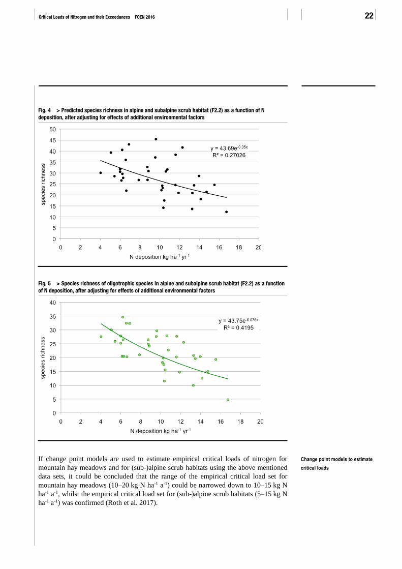
Fig. 4 > Predicted species richness in alpine and subalpine scrub habitat (F2.2) as a function of N deposition, after adjusting for effects of additional environmental factors
Fig. 5 > Species richness of oligotrophic species in alpine and subalpine scrub habitat (F2.2) as a function of N deposition, after adjusting for effects of additional environmental factors
If change point models are used to estimate empirical critical loads of nitrogen for
mountain hay meadows and for (sub-)alpine scrub habitats using the above mentioned
data sets, it could be concluded that the range of the empirical critical load set for
mountain hay meadows (10–20 kg N ha-1 a-1) could be narrowed down to 10–15 kg N
ha-1 a-1, whilst the empirical critical load set for (sub-)alpine scrub habitats (5–15 kg N
ha-1 a-1) was confirmed (Roth et al. 2017).
Change point models to estimate
critical loads

2 > Methods to Derive Critical Loads of Nutrient Nitrogen 23
In alpine and subalpine scrub habitats (F2.2) the exposure-response relationships for
total species richness and for species richness of oligotrophic species are very similar
(Figure 4, Figure 5). This is not surprising, since on average 79 ± 13% of all species
belong to the oligotrophic species. The effect of relatively small doses, especially on
oligotrophic species, is in accordance with recent studies in other alpine habitats, where
the proportional biomass of functional groups changed by the addition of 5 kg N ha-1a-1
(Bassin et al. 2013).
2.2.3 Mapping Empirical Critical Loads for Ecosystems in Switzerland
For the purpose of applying the empirical critical loads approach, countries have to
identify those receptors or ecosystems of maximum sensitivity from the list of ecosys-
tem types of Table 1 relating to their individual priorities to protect the environment.
Table 2 and Table 3 present the ecosystems for which the empirical critical load ap-
proach was applied in Switzerland. Table 3 specifically addresses dry grassland
(TWW).
The selection of sensitive ecosystems to be protected by applying the empirical method
is based on ecosystem and vegetation data compiled from various sources described
below. All of the selected ecosystems are of high conservation importance with respect
to biodiversity, landscape quality and ecosystem services. They include natural as well
as semi-natural ecosystem types. Overall, 45 sensitive ecosystem types according to
EUNIS classes were identified and included in the critical load data set:
> 21 various so-called “types of vegetation worthy of protection” from the vegetation
atlas by Hegg et al. (1993) including rare and species-rich forest types, alpine
heaths, grasslands and surface waters (see Tab. 2). The atlas contains distribution
maps for 97 vegetation types with a resolution of 1 x 1 km². 21 vegetation types sen-
sitive to eutrophication were selected.
> 1 type of mountain hay meadow (see Tab. 2) in montane to sub-alpine altitudinal
zones with more than 35 species per 10 m² (Roth et al. 2013). This applies to 122
sites of the Swiss Biodiversity Monitoring (BDM, indicator Z910).
> 1 type of raised bog from the Federal Inventory of Raised and Transitional Bogs of
National Importance (Appendix to Swiss Confederation 1991) (see Tab. 2). This
data set is available in vector format at a scale of 1:25 000. The inventory contains
only bogs with relevant occurrences of sphagnion fusci.
> 3 types of poor or rich fens from the Federal Inventory of Fenlands of National
Importance (Appendix to Swiss Confederation 1994, WSL 1993) (see Tab. 2). This
data set is available in vector format at a scale of 1:25 000. For the maps compiled
by the Coordination Centre for Effects (UNECE), only the mesotrophic fens were
selected. Eutrophic fens, such as Phragmition, Magnocaricon, Molinion and Calthi-
on were omitted.
> 1 type of oligotrophic alpine lakes (see Tab. 2). The catchments of 100 lakes in
Southern Switzerland at altitudes between 1650 and 2700 m (average 2200 m) were
mapped by Posch et al. 2007. To a large extent the selected catchments consist of
crystalline bedrock and are therefore sensitive to acidification and eutrophication.
10 www.biodiversitymonitoring.ch/en/data/indicators/z/z9.html
Selection of sensitive ecosystems
Critical Loads of Nitrogen and their Exceedances FOEN 2016 24
> 18 types of dry grassland (TWW) from the National Inventory of Dry Grasslands of
National Importance (Eggenberg et al. 2001, FOEN 2007) (see Tab. 3). This data set
is available in vector format at a scale of 1:25 000. Many of those grasslands are
extensively managed as hay meadows. They also include alpine and subalpine grass-
land.
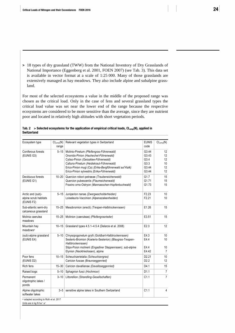
For most of the selected ecosystems a value in the middle of the proposed range was
chosen as the critical load. Only in the case of fens and several grassland types the
critical load value was set near the lower end of the range because the respective
ecosystems are considered to be more sensitive than the average, since they are nutrient
poor and located in relatively high altitudes with short vegetation periods.
Tab. 2 > Selected ecosystems for the application of empirical critical loads, CLemp(N), applied in Switzerland
Ecosystem type CLemp(N)
range
Relevant vegetation types in Switzerland EUNIS
code
CLemp(N)
Coniferous forests
(EUNIS G3)
5–15
Molinio-Pinetum (Pfeifengras-Föhrenwald)
Ononido-Pinion (Hauhechel-Föhrenwald)
Cytiso-Pinion (Geissklee-Föhrenwald)
Calluno-Pinetum (Heidekraut-Föhrenwald)
Erico-Pinion mugi (Ca) (Erika-Bergföhrenwald auf Kalk)
Erico-Pinion sylvestris (Erika-Föhrenwald)
G3.44
G3.43
G3.4
G3.3
G3.44
G3.44
12
12
12
10
12
12
Deciduous forests
(EUNIS G1)
10–20 Quercion robori-petraeae (Traubeneichenwald)
Quercion pubescentis (Flaumeichenwald)
Fraxino orno-Ostryon (Mannaeschen-Hopfenbuchwald)
G1.7
G1.71
G1.73
15
15
15
Arctic and (sub)-
alpine scrub habitats
(EUNIS F2)
5–15
Juniperion nanae (Zwergwacholderheiden)
Loiseleurio-Vaccinion (Alpenazaleenheiden)
F2.23
F2.21
10
10
Sub-atlantic semi-dry
calcareous grassland
15–25 Mesobromion (erecti) (Trespen-Halbtrockenrasen) E1.26 15
Molinia caerulea
meadows
15–25 Molinion (caeruleae) (Pfeifengrasrieder) E3.51 15
Mountain hay
meadowsa
10–15
Grassland types 4.5.1–4.5.4 (Delarze et al. 2008) E2.3 12
(sub)-alpine grassland
(EUNIS E4)
5–10 Chrysopogonetum grylli (Goldbart-Halbtrockenrasen)
Seslerio-Bromion (Koelerio-Seslerion) (Blaugras-Trespen-
Halbtrockenrasen)
Stipo-Poion molinerii (Engadiner Steppenrasen), sub-alpine
Elynion (Nacktriedrasen), alpine
E4.3
E4.4
E4.4
E4.42
10
10
10
7
Poor fens
(EUNIS D2)
10–15 Scheuchzerietalia (Scheuchzergras)
Caricion fuscae (Braunseggenried)
D2.21
D2.2
10
12
Rich fens 15–30 Caricion davallianae (Davallsseggenried) D4.1 15
Raised bogs 5–10 Sphagnion fusci (Hochmoor) D1.1 7
Permanent
oligotrophic lakes /
ponds
3–10 Littorellion (Strandling-Gesellschaften) C1.1 7
Alpine oligotrophic
softwater lakes
3–5 sensitive alpine lakes in Southern Switzerland C1.1 4
a) adapted according to Roth et al. 2017
Units are in kg N ha-1 a-1

2 > Methods to Derive Critical Loads of Nutrient Nitrogen 25
Tab. 3 > Empirical critical loads of nitrogen, CLemp(N), assigned to dry grasslands (TWW) of the National Inventory of Dry Grasslands
In kg N ha-1 a-1.
TWW-code Vegetation type
EUNIS Remarks CLemp(N)
1 CA Caricion austro-alpinae
(Südalpine Blaugrashalde)
E4.4 (sub-)alpine grassland 8
2 CB Cirsio-Brachypodion
(Subkontinentaler Trockenrasen)
E1.23 similar to TWW 18 (Mesobromion), also
used as hay meadow
12
3 FP Festucion paniculatae
(Goldschwingelhalde)
E4.3 similar to TWW 13 (Festucion variae); also
mapped by Hegg et al.
7
4 LL low diversity, low altitude grassland
(artenarme Trockenrasen der
tieferen Lagen)
E2.2 contains different types, promising
diversity when mown, therefore lower
range chosen
15
5 AI Agropyrion intermedia
(Halbruderaler Trockenrasen)
E1.2 transitional type 15
6 SP Stipo-Poion
(Steppenartiger Trockenrasen)
E1.24 pastures/fallows in large inner-alpine
valleys; CLemp(N) based on national
expert-judgment (Hegg et al. 1993)
10
7 MBSP Mesobromion / Stipo-Poion
(Steppenartiger Halbtrockenrasen)
E1.26 pastures, slightly more nutrient-rich than
Mesobromion (TWW18)
15
8 XB Xerobromion
(Subatlantischer Trockenrasen)
E1.27 meadows/pastures/fallows in large inner-
alpine valleys; CLemp(N) based on national
expert-judgment (Hegg et al. 1993)
12
9 MBXB Mesobromion/Xerobromion
(Trockener Halbrockenrasen)
E1.26 similar to TWW 18 (Mesobromion) 12
10 LH low diversity, high altitude grassland
(artenarme Trockenrasen der
höheren Lagen)
E2.3 contains different types of dry grassland at
high altitude
12
11 CF Caricion ferrugineae
(Rostseggenhalde)
E4.41 (sub-)alpine grassland; also mapped by
Hegg et al.
7
12 AE Arrhenatherion elatioris
(Trockene artenreiche Fettwiese)
E2.2 often used as meadows, lower range
chosen as it occurs at all altitude levels
12
13 FV Festucion variae
(Buntschwingelhalde)
E4.3 (sub-)alpine grassland, middle of the
range chosen
7
14 SV Seslerion variae
(Blaugrashalde)
E4.43 alpine grassland, middle of the range
chosen; also mapped by Hegg et al.
7
15 NS Nardion strictae
(Borstgrasrasen)
E1.71 meadows, subalpine 12
16 OR Origanietalia
(Trockene Saumgesellschaft)
E2.3 meadows/fallows 15
17 MBAE Mesobromion/Arrhenatherion
(Nährstoffreicher Halbtrockenrasen)
E1.26 slightly more nutrient-rich than
Mesobromion (TWW18)
15
18 MB Mesobromion
(Echter Halbrockenrasen)
E1.26 genuine semi-dry grassland 12
Eggenberg et al. 2001, FOEN 2007

Critical Loads of Nitrogen and their Exceedances FOEN 2016 26
Raised bogs, oligotrophic ponds, alpine grassland, alpine heaths and most of the select-
ed forest types are (semi-)natural ecosystems, i.e. they are not managed or only poorly
managed.
Fens and species-rich grassland below the alpine level are semi-natural systems, in
general. They developed under permanent traditional management over centuries.
When these extensive forms of management change, the ecosystems generally show a
decrease in biodiversity.
The TWW data set complements well the grassland types mapped by Hegg et al.
(1993). It contains 18 vegetation groups, which partially also occur in the inventory of
Hegg. The two inventories are used here in a complementary way, because they fulfil
different purposes: The atlas by Hegg gives an overview of the occurrence of selected
vegetation types, while TWW focuses on the precise description of sites with national
importance.
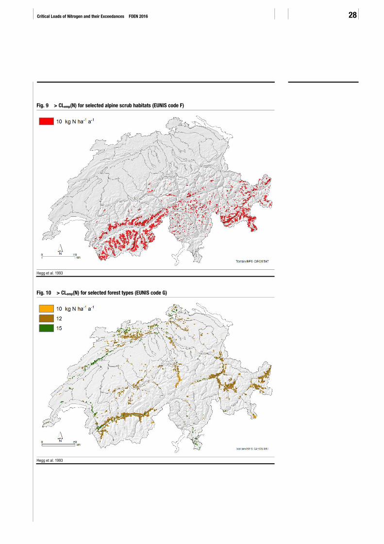
For the data and maps used under the Convention on Long-range Transboundary Air
Pollution and submitted to the Coordination Centre for Effects, the outlines of all
ecosystem-specific polygons (in vector format) were converted to a 1 x 1 km² grid
(present / absent criterion). If more than one ecosystem type occurs within a 1 x 1 km²
grid-cell, the lowest value of CLemp(N) was selected for this cell. The spatial distribu-
tion of the selected ecosystem types and their CLemp(N) according to Table 2 and
Table 3 are shown on the maps in Figure 6 to Figure 10.
Fig. 6 > CLemp(N) for oligotrophic surface waters (EUNIS code C)
Hegg et al. 1993, Posch et al. 2007

2 > Methods to Derive Critical Loads of Nutrient Nitrogen 27
Fig. 7 > CLemp(N) for raised bogs and fens (EUNIS code D)
Swiss Confederation 1991 and 1994
Fig. 8 > CLemp(N) for selected grassland types (EUNIS code E)
Hegg et al. 1993, TWW, BDM
Critical Loads of Nitrogen and their Exceedances FOEN 2016 28
Fig. 9 > CLemp(N) for selected alpine scrub habitats (EUNIS code F)
Hegg et al. 1993
Fig. 10 > CLemp(N) for selected forest types (EUNIS code G)
Hegg et al. 1993

2 > Methods to Derive Critical Loads of Nutrient Nitrogen 29
2.3 The Simple Mass Balance Method (SMB)
In Switzerland, the SMB method was applied for productive forest ecosystems, i.e.
sites where wood harvesting is possible.
2.3.1 The Calculation Method
The SMB method for calculating critical loads of nutrient nitrogen is a steady-state
model based on the nitrogen saturation concept. There are several definitions of N
saturation. In this context it is understood as follows: The atmospheric nitrogen deposi-
tion must not lead to a situation where the availability of inorganic nitrogen is in excess
of the total combined plant and microbial nutritional demand. I.e. the inputs should not
be larger than the natural sinks plus outputs.
The basic principle of the SMB method is to identify the long-term average sources
and sinks of inorganic nitrogen in the system, and to determine the maximum tolerable
nitrogen input that will protect the system from nitrogen saturation. The nitrogen
cycling within the ecosystems is mainly regulated by biological processes that depend
on the following factors: (1) the ecosystem type, (2) former and present land use and
management, (3) environmental conditions, especially those influencing the nitrifica-
tion rate and the immobilization rate. Consequently these factors are important for
calculating and setting critical loads of nutrient nitrogen.
In the mapping manual (UNECE 2016) a simplified SMB equation is formulated as
follows:
CLnut(N) = Ni + Nu + Nde + Nle(acc)
Where:
CLnut(N) critical load of nutrient nitrogen [kg N ha-1 a-1].
Ni = acceptable immobilization rate of N in soil organic matter (including forest
floor) at N inputs equal to critical load, at which adverse ecosystem change will
not take place [kg N ha-1 a-1].
Nu nitrogen uptake; net removal of nitrogen in vegetation at critical load [kg N ha-1
a-1]. This is the amount of nitrogen which is removed from the system by (wood)
harvesting.
Nde denitrification rate [kg N ha-1 a-1]. This is the flux to the atmosphere of gaseous
compounds (N2, N2O and NO) produced by microorganisms (mainly under
anaerobic conditions) in the soil.
Nle(acc) acceptable total nitrogen leaching from the rooting zone at which no damage
occurs in the terrestrial or linked ecosystem plus any enhanced leaching
following forest harvesting [kg N ha-1 a-1]. This is the N removed from the soil
by the vertically percolating water flux.
Principle of the Simple Mass
Balance (SMB)
2.1

Critical Loads of Nitrogen and their Exceedances FOEN 2016 30
The equation is based on the following assumptions:
> All rates and fluxes of the involved processes are represented by annual means.
> Temporal variations in Nu as a function of forest age and management are not
included, i.e. the temporal scale of the investigation is longer than one rotation peri-
od (>100 years).
> Nitrogen losses by natural fires, erosion and ammonia volatilisation as well as
biological N fixation are negligible in most Swiss forests.
Equation 2.1 as such is not operational, as Nde strongly depends on nitrogen deposition.
The mapping manual proposes to use linear or non-linear functions to calculate Nde.
For the application in Switzerland the constant function is used:
Nde = fde ( Ndep – Nu – Ni )
if Ndep > Nu + Ni
Nde = 0 otherwise
Where:
fde denitrification fraction.
Ndep nitrogen deposition [kg N ha-1 a-1].
This formulation implicitly assumes that immobilization and uptake are faster process-
es than denitrification. Under critical load conditions Ndep is equal to CLnut(N). By
inserting equation 2.2 into 2.1 the critical load becomes:
CLnut(N) = Ni +Nu + Nle(acc) / ( 1 – fde )
Maps of critical loads to be used under the Convention on LRTAP were produced in
two steps:
In a first step, equation 2.3 was applied for 10 331 sites of the National Forest Invento-
ry NFI (WSL 1990/92, EAFV 1988) located on a 1 x 1 km² raster, and for 301 forest
sites used in dynamic modelling (Achermann et al. 2015). Thereby, only NFI-sites with
a defined mixing ratio of deciduous and coniferous trees are included. This corresponds
approximately to the productive forest area as unproductive and unmanaged woodlands
such as brush forests and inaccessible forests are excluded.
In a second step, the lower limit of CLnut(N) calculated by the SMB was set to 10 kg N
ha-1 a-1 (corresponding to the lower limit of CLemp(N) used for forests). This means, all
values of CLnut(N) below 10 kg N ha-1 a-1 were set to 10. This was done with respect to
the fact that so far no empirically observed harmful effects in forest ecosystems were
published for depositions lower than 10 kg N ha-1 a-1 and for latitudes and altitudes
2.2
2.3
Application of the SMB method
for forest sites
2 > Methods to Derive Critical Loads of Nutrient Nitrogen 31
typical for Switzerland. Therefore, the critical loads calculated with the SMB method
were adjusted to empirically confirmed values.
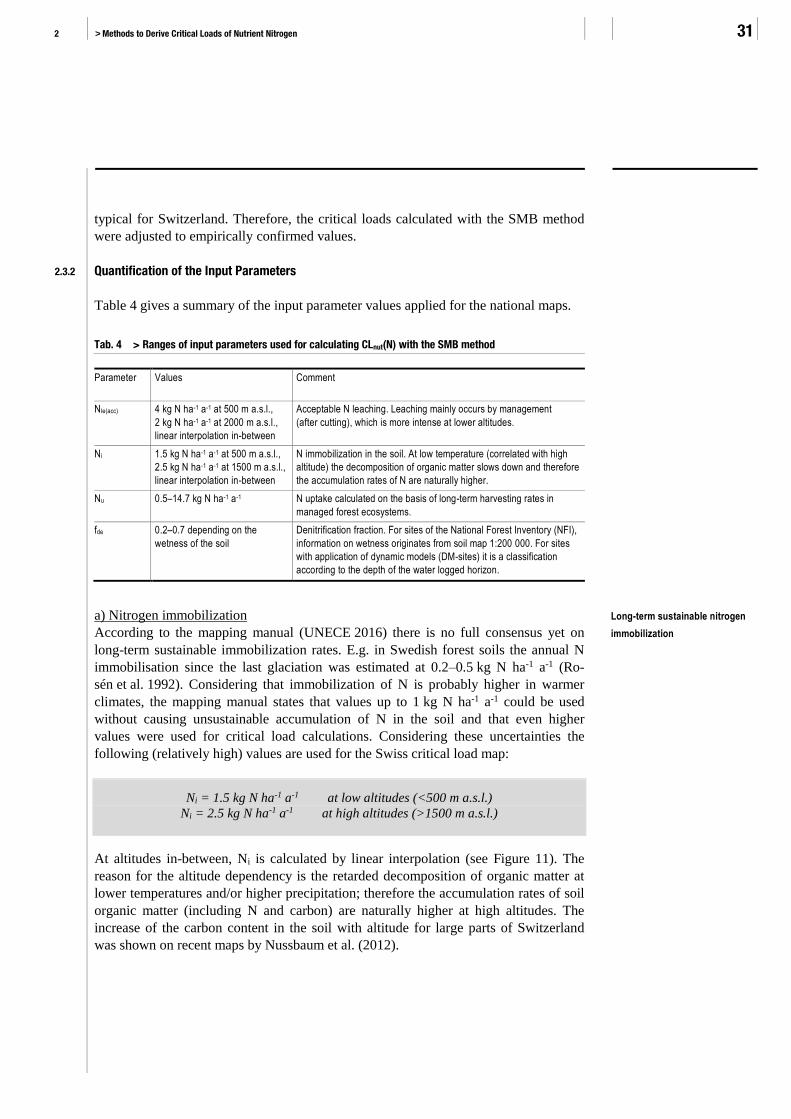
2.3.2 Quantification of the Input Parameters
Table 4 gives a summary of the input parameter values applied for the national maps.
Tab. 4 > Ranges of input parameters used for calculating CLnut(N) with the SMB method
Parameter Values
Comment
Nle(acc) 4 kg N ha-1 a-1 at 500 m a.s.l.,
2 kg N ha-1 a-1 at 2000 m a.s.l.,
linear interpolation in-between
Acceptable N leaching. Leaching mainly occurs by management
(after cutting), which is more intense at lower altitudes.
Ni 1.5 kg N ha-1 a-1 at 500 m a.s.l.,
2.5 kg N ha-1 a-1 at 1500 m a.s.l.,
linear interpolation in-between
N immobilization in the soil. At low temperature (correlated with high
altitude) the decomposition of organic matter slows down and therefore
the accumulation rates of N are naturally higher.
Nu 0.5–14.7 kg N ha-1 a-1 N uptake calculated on the basis of long-term harvesting rates in
managed forest ecosystems.
fde 0.2–0.7 depending on the
wetness of the soil
Denitrification fraction. For sites of the National Forest Inventory (NFI),
information on wetness originates from soil map 1:200 000. For sites
with application of dynamic models (DM-sites) it is a classification
according to the depth of the water logged horizon.
a) Nitrogen immobilization
According to the mapping manual (UNECE 2016) there is no full consensus yet on
long-term sustainable immobilization rates. E.g. in Swedish forest soils the annual N
immobilisation since the last glaciation was estimated at 0.2–0.5 kg N ha-1 a-1 (Ro-
sén et al. 1992). Considering that immobilization of N is probably higher in warmer
climates, the mapping manual states that values up to 1 kg N ha-1 a-1 could be used
without causing unsustainable accumulation of N in the soil and that even higher
values were used for critical load calculations. Considering these uncertainties the
following (relatively high) values are used for the Swiss critical load map:
Ni = 1.5 kg N ha-1 a-1 at low altitudes (<500 m a.s.l.)
Ni = 2.5 kg N ha-1 a-1 at high altitudes (>1500 m a.s.l.)
At altitudes in-between, Ni is calculated by linear interpolation (see Figure 11). The
reason for the altitude dependency is the retarded decomposition of organic matter at
lower temperatures and/or higher precipitation; therefore the accumulation rates of soil
organic matter (including N and carbon) are naturally higher at high altitudes. The
increase of the carbon content in the soil with altitude for large parts of Switzerland
was shown on recent maps by Nussbaum et al. (2012).
Long-term sustainable nitrogen
immobilization

Critical Loads of Nitrogen and their Exceedances FOEN 2016 32
Fig. 11 > Nitrogen immobilization values for forest soils used for the SMB method on the 1 x 1 km² raster
b) Nitrogen uptake
Nitrogen and base cations (Ca, Mg, K, Na) are taken up by trees and used for biomass
production. In unmanaged forests at steady state, the net uptake will be zero since
biomass production is in balance with biomass decomposition. In a managed forest, the
net uptake rate is obtained by multiplying the long-term net growth (harvesting) rate
with nitrogen and cation contents of the wood.
For the 301 sites used in dynamic modelling (DM-sites), Kurz & Posch (2015) mod-
elled net-uptake fluxes with MakeDep (Alveteg et al. 2002) using biomass data from
the third National Forest Inventory (NFI, WSL 2013), tree genera-specific logistic
growth curves, site productivity index, nutrient contents in the various compartments of
the tree, and average annual harvesting rates (FOEN 2013). MakeDep is able to con-
sider the mutual dependence of deposition, forest canopy growth/size and nutrient
demand of the growing forest.
Harvesting rates were stratified according to the five NFI-regions: Jura, Central Plat-
eau, Pre-Alps, Alps and Southern Alps. The harvesting rates before 2000 add up to 4.5
million m³ stem wood, which is in the range of the typical annual harvest in Switzer-
land (in years without heavy storms); after 2000, the harvest of energy wood slightly
increased and the average harvest was around 5.0 million m³ (FOEN 2013).
The nitrogen uptake for the forest sites on the 1 x 1 km² raster was derived from the
results at the DM-sites by linear regressions with altitude (z); the regression analysis
was stratified according to the five NFI-regions (Table 5, Figure 12). In the Jura and
Central Plateau regions, the average harvesting rates reach the long-term gross growth,
but in the mountainous and southern parts of Switzerland it is much lower than gross
Nitrogen uptake

2 > Methods to Derive Critical Loads of Nutrient Nitrogen 33
growth. The resulting uptake values are in the range from 1.0 to 8.8 kg N ha-1a-1 (see
Figure 12).
Tab. 5 > Net nitrogen uptake (Nu) in the five NFI-regions (kg N ha-1 a-1)
Region Average Function of altitude z
(m a.s.l.)
1. Jura 5.3 6.99–0.00300 z
2. Central Plateau 8.5 8.5
3. Pre-Alps 4.3 7.60–0.00322 z
4. Alps 2.9 3.58–0.00064 z
5. Southern Alps 1.6 2.29–0.00056 z
Average CH 4.4 -
Fig. 12 > Net nitrogen uptake (Nu) of managed forest ecosystems used for the SMB method on the 1 x 1 km² raster
c) Nitrogen leaching
Within the scope of the CCE data-call 2007, the National Focal Centres were requested
to reassess their CLnut(N) calculations and update them if appropriate based on revised
critical N concentrations (cNacc) (UNECE 2013, chapter 5.3.1.2). For Switzerland, the
proposed values for cNacc were tested (see Achermann et al. 2007). Some of the
proposed values led to implausible high N leaching and CLnut(N), mainly in high
precipitation areas.
Therefore it was decided to continue using the acceptable N leaching rates (Nle[acc]),
which were used already in former data submissions. They are basically drawn from
earlier versions of the Mapping Manual (UNECE 1996) and on findings of the work-
Acceptable nitrogen leaching

Critical Loads of Nitrogen and their Exceedances FOEN 2016 34
shop on critical loads for nitrogen held in Lökeberg in 1992 (Grennfelt and Thörnelöf
1992):
Nle(acc) = 4 kg N ha-1 a-1 at low altitudes (<500 m a.s.l.)
Nle(acc) = 2 kg N ha-1 a-1 at high altitudes (>2000 m a.s.l.)
At altitudes in-between, Nle(acc) is calculated by linear interpolation. The rationale for
this procedure is that acceptable leaching mainly occurs after disturbances by manage-
ment (cutting), which is more intense at lower altitudes. The resulting map is shown in
Figure 13.
Fig. 13 > Acceptable nitrogen leaching values of forest ecosystems used for the SMB method on the 1 x 1 km² raster
d) Denitrification fraction
The fde values proposed in the mapping manual (UNECE 2016) are between 0.0 and
0.8. There are two proposals for relating fde values to different soil properties:
> Soil types: for sandy soils without gleyic features or loess a value of 0.0–0.1, for
sandy soils with gleyic features 0.5, for clay soils 0.7, for peat soils 0.8.
> Soil drainage status: excessive 0.0, good 0.1, moderate 0.2, imperfect 0.4, poor 0.7,
very poor 0.8.
For calculating CLnut(N) at the 1 x 1 km² raster of the National Forest Inventory), fde
was determined according to wetness information from the digital soil map BEK
(SFSO 2000) as shown in Table 6 and Figure 14.
Denitrification
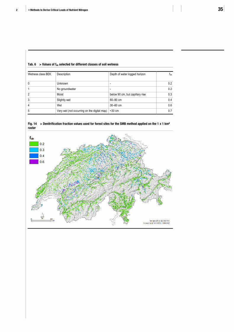
2 > Methods to Derive Critical Loads of Nutrient Nitrogen 35
Tab. 6 > Values of fde selected for different classes of soil wetness
Wetness class BEK
Description Depth of water logged horizon fde
0 Unknown - 0.2
1 No groundwater - 0.2
2 Moist below 90 cm, but capillary rise 0.3
3 Slightly wet 60–90 cm 0.4
4 Wet 30–60 cm 0.6
5 Very wet (not occurring on the digital map) <30 cm 0.7
Fig. 14 > Denitrification fraction values used for forest sites for the SMB method applied on the 1 x 1 km² raster
Critical Loads of Nitrogen and their Exceedances FOEN 2016 36
3 > Mapping Nitrogen Deposition - - - - - - - - - - - - - - - - - - - - - - - - - - - - - - - - - - - - - - - - - - - - - - - - - - - - - - - - - - - - - - - - - - - - - - - - - - - - - - - - - - - - - - - - - - - - - - - - - - - - - - - - - - - - - - -
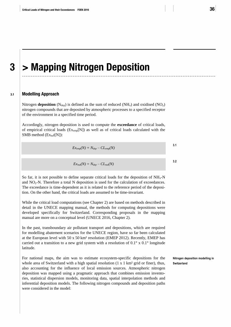
3.1 Modelling Approach
Nitrogen deposition (Ndep) is defined as the sum of reduced (NHx) and oxidised (NOy)
nitrogen compounds that are deposited by atmospheric processes to a specified receptor
of the environment in a specified time period.
Accordingly, nitrogen deposition is used to compute the exceedance of critical loads,
of empirical critical loads (Exemp[N]) as well as of critical loads calculated with the
SMB method (Exnut[N]):
Exemp(N) = Ndep – CLemp(N)
Exnut(N) = Ndep – CLnut(N)
So far, it is not possible to define separate critical loads for the deposition of NHx-N
and NOy-N. Therefore a total N deposition is used for the calculation of exceedances.
The exceedance is time-dependent as it is related to the reference period of the deposi-
tion. On the other hand, the critical loads are assumed to be time-invariant.
While the critical load computations (see Chapter 2) are based on methods described in
detail in the UNECE mapping manual, the methods for computing depositions were
developed specifically for Switzerland. Corresponding proposals in the mapping
manual are more on a conceptual level (UNECE 2016, Chapter 2).
In the past, transboundary air pollutant transport and depositions, which are required
for modelling abatement scenarios for the UNECE region, have so far been calculated
at the European level with 50 x 50 km² resolution (EMEP 2012). Recently, EMEP has
carried out a transition to a new grid system with a resolution of 0.1° x 0.1° longitude
latitude.
For national maps, the aim was to estimate ecosystem-specific depositions for the
whole area of Switzerland with a high spatial resolution (1 x 1 km² grid or finer), thus,
also accounting for the influence of local emission sources. Atmospheric nitrogen
deposition was mapped using a pragmatic approach that combines emission invento-
ries, statistical dispersion models, monitoring data, spatial interpolation methods and
inferential deposition models. The following nitrogen compounds and deposition paths
were considered in the model:
3.1
3.2
Nitrogen deposition modelling in
Switzerland

3 > Mapping Nitrogen Deposition 37
> wet deposition of nitrate (NO3-) and ammonium (NH4
+);
> dry deposition of gaseous ammonia (NH3), nitrogen dioxide (NO2) and nitric acid
(HNO3);
> dry deposition of particulate nitrate and ammonium (secondary aerosols).
As shown in Figure 15, concentrations of the primary gaseous pollutants (NH3 and
NO2) are modelled by means of emission maps and statistical dispersion models with a
resolution of 100 x 100 m². Thus, the high spatial variability of these pollutants nearby
emission sources can be reflected in the models. The concentrations of secondary
pollutants (aerosols, HNO3) as well as the concentrations of N in precipitation are
derived from field monitoring data by applying geo-statistical interpolation methods.
Wet deposition is calculated by combining the concentration field of N compounds in
rainwater with the precipitation amount (5-year-averages), see Chapter 3.2.
“Inferential” models are used for assessing the dry deposition of gases and aerosols:
The concentration maps are multiplied with deposition velocities (Vdep), which depend
on the reactivity of the pollutant, the surface roughness and climatic parameters (Chap-
ter 3.3). Values of Vdep were taken from literature. “Occult” deposition through cloud
water or fog is not taken into account.
Maps of emissions, concentrations and deposition were calculated for the years 1990,
2000, 2007 and 2010. For 2000, 2007 and 2010 identical methods were used, i.e. it is a
homogenous time series. For the year 1990, a somewhat modified method adapted to
the availability of data was applied. The following chapters present the approach and
input data used for the year 2010.
Fig. 15 > Deposition modelling scheme
based on figure by Hertel et al. 2011
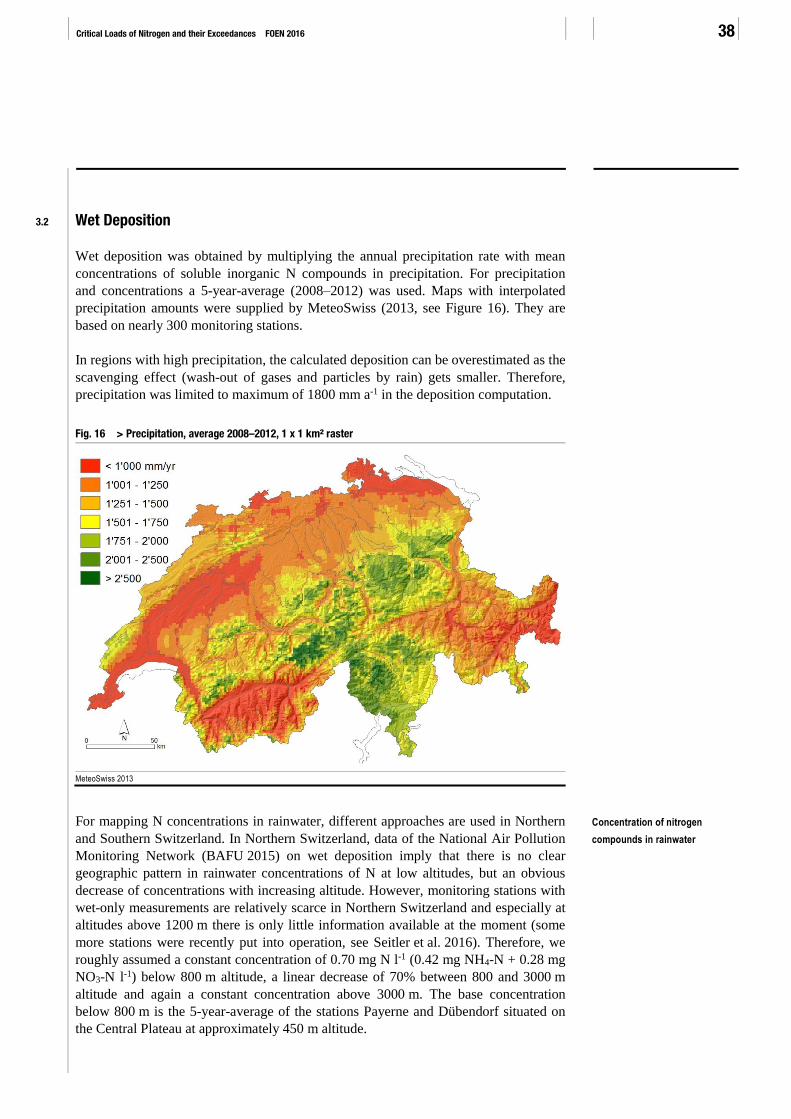
Critical Loads of Nitrogen and their Exceedances FOEN 2016 38
3.2 Wet Deposition
Wet deposition was obtained by multiplying the annual precipitation rate with mean
concentrations of soluble inorganic N compounds in precipitation. For precipitation
and concentrations a 5-year-average (2008–2012) was used. Maps with interpolated
precipitation amounts were supplied by MeteoSwiss (2013, see Figure 16). They are
based on nearly 300 monitoring stations.
In regions with high precipitation, the calculated deposition can be overestimated as the
scavenging effect (wash-out of gases and particles by rain) gets smaller. Therefore,
precipitation was limited to maximum of 1800 mm a-1 in the deposition computation.
Fig. 16 > Precipitation, average 2008–2012, 1 x 1 km² raster
MeteoSwiss 2013
For mapping N concentrations in rainwater, different approaches are used in Northern
and Southern Switzerland. In Northern Switzerland, data of the National Air Pollution
Monitoring Network (BAFU 2015) on wet deposition imply that there is no clear
geographic pattern in rainwater concentrations of N at low altitudes, but an obvious
decrease of concentrations with increasing altitude. However, monitoring stations with
wet-only measurements are relatively scarce in Northern Switzerland and especially at
altitudes above 1200 m there is only little information available at the moment (some
more stations were recently put into operation, see Seitler et al. 2016). Therefore, we
roughly assumed a constant concentration of 0.70 mg N l-1 (0.42 mg NH4-N + 0.28 mg
NO3-N l-1) below 800 m altitude, a linear decrease of 70% between 800 and 3000 m
altitude and again a constant concentration above 3000 m. The base concentration
below 800 m is the 5-year-average of the stations Payerne and Dübendorf situated on
the Central Plateau at approximately 450 m altitude.
Concentration of nitrogen
compounds in rainwater

3 > Mapping Nitrogen Deposition 39
The assumptions related to the decrease in concentrations between 800 and 3000 m
altitude were adjusted during the last years based on comparisons with measurements
carried out at higher altitudes on Swiss Long-term Forest Ecosystem Research plots
(Thimonier et al. 2005) and on Alpine grassland (Hiltbrunner et al. 2005).
In Southern Switzerland, there are several stations run by the Canton Ticino besides
NABEL and neighbouring Italian stations. Thus, the wet-only monitoring network is
relatively dense. Concentrations in rainwater and deposition maps were calculated by
regression models considering longitude, latitude and altitude. They were initially
developed by Barbieri & Pozzi (2001) and updated by Steingruber & Colombo (2010)
and Steingruber (2014). For the period 2008–2012, ammonium and nitrate concentra-
tions in precipitation can be calculated for the region of the Canton Ticino as follows:
Cwet(NH4+) = -22.4 + 0.0001238 x – 0.0002581 y – 0.00461 z
Cwet(NO3-) = -66.4 + 0.0001581 x – 0.0001366 y – 0.00292 z
where:
Cwet(N) concentration of N-compound in rainwater [meq m-3].
x, y longitude/latitude in Swiss projection LV0311 (m).
z altitude (m).
The resulting concentration maps are shown in Figure 17.
Fig. 17 > Concentration in rainwater of ammonium (left) and nitrate (right), average 2008–2012, 1 x 1 km² raster
11 www.swisstopo.admin.ch/internet/swisstopo/en/home/topics/survey/sys/refsys/projections.html
3.3
3.4
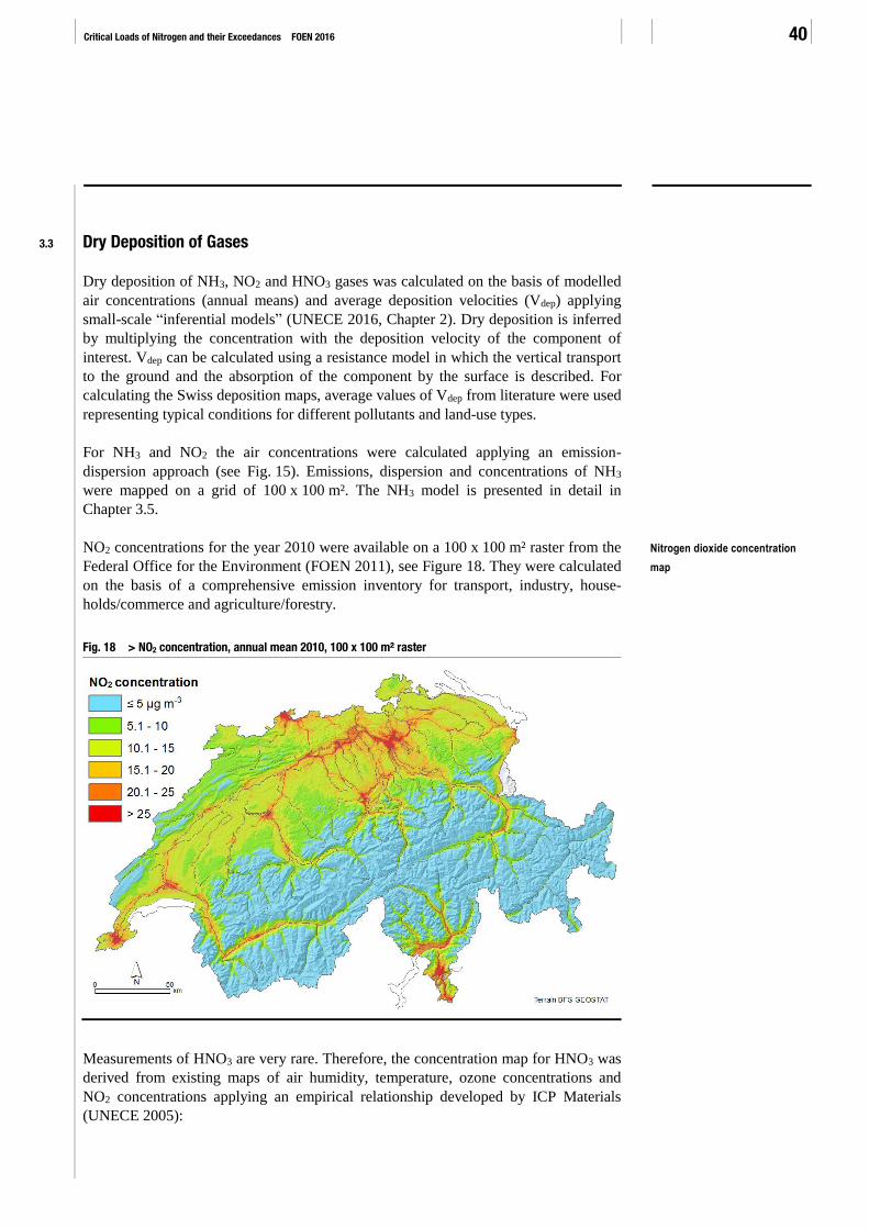
Critical Loads of Nitrogen and their Exceedances FOEN 2016 40
3.3 Dry Deposition of Gases
Dry deposition of NH3, NO2 and HNO3 gases was calculated on the basis of modelled
air concentrations (annual means) and average deposition velocities (Vdep) applying
small-scale “inferential models” (UNECE 2016, Chapter 2). Dry deposition is inferred
by multiplying the concentration with the deposition velocity of the component of
interest. Vdep can be calculated using a resistance model in which the vertical transport
to the ground and the absorption of the component by the surface is described. For
calculating the Swiss deposition maps, average values of Vdep from literature were used
representing typical conditions for different pollutants and land-use types.
For NH3 and NO2 the air concentrations were calculated applying an emission-
dispersion approach (see Fig. 15). Emissions, dispersion and concentrations of NH3
were mapped on a grid of 100 x 100 m². The NH3 model is presented in detail in
Chapter 3.5.
NO2 concentrations for the year 2010 were available on a 100 x 100 m² raster from the
Federal Office for the Environment (FOEN 2011), see Figure 18. They were calculated
on the basis of a comprehensive emission inventory for transport, industry, house-
holds/commerce and agriculture/forestry.
Fig. 18 > NO2 concentration, annual mean 2010, 100 x 100 m² raster
Measurements of HNO3 are very rare. Therefore, the concentration map for HNO3 was
derived from existing maps of air humidity, temperature, ozone concentrations and
NO2 concentrations applying an empirical relationship developed by ICP Materials
(UNECE 2005):
Nitrogen dioxide concentration
map
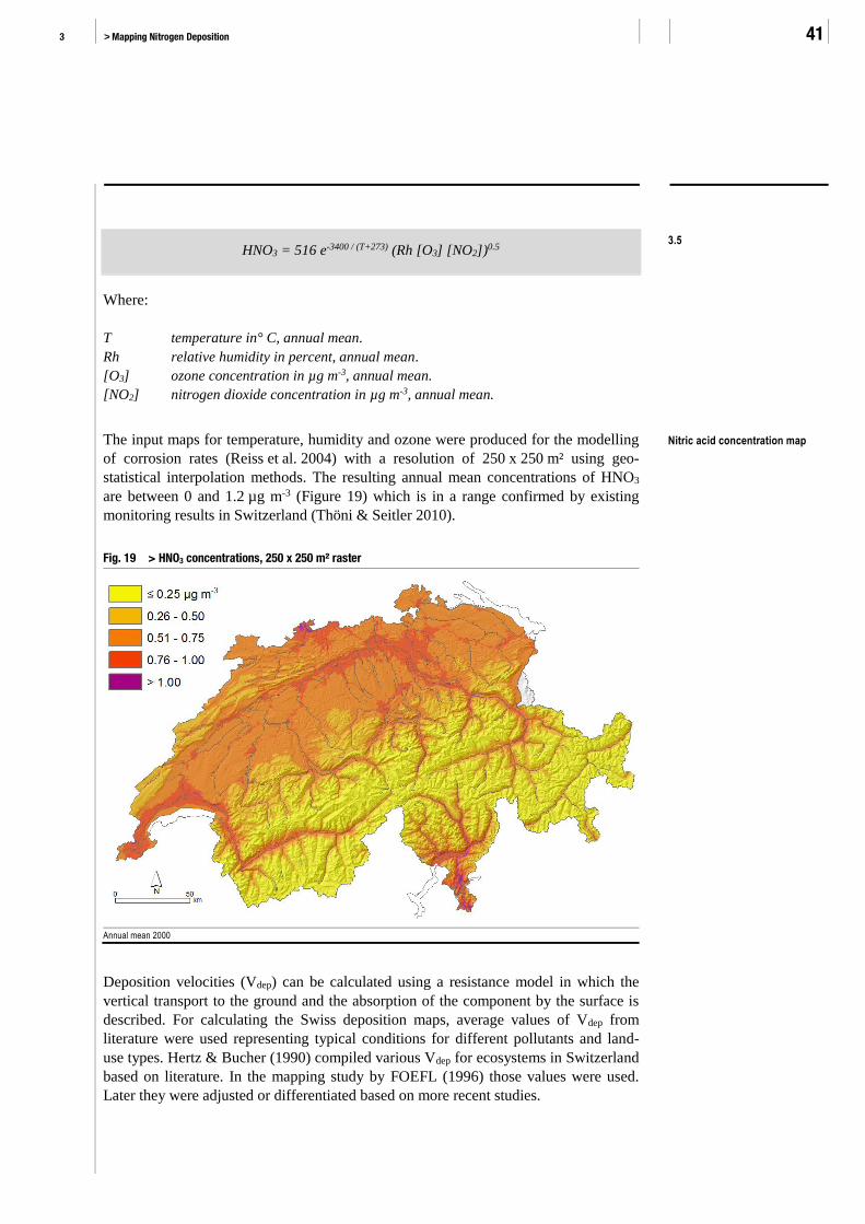
3 > Mapping Nitrogen Deposition 41
HNO3 = 516 e-3400 / (T+273) (Rh [O3] [NO2])0.5
Where:
T temperature in° C, annual mean.
Rh relative humidity in percent, annual mean.
[O3] ozone concentration in µg m-3, annual mean.
[NO2] nitrogen dioxide concentration in µg m-3, annual mean.
The input maps for temperature, humidity and ozone were produced for the modelling
of corrosion rates (Reiss et al. 2004) with a resolution of 250 x 250 m² using geo-
statistical interpolation methods. The resulting annual mean concentrations of HNO3
are between 0 and 1.2 µg m-3 (Figure 19) which is in a range confirmed by existing
monitoring results in Switzerland (Thöni & Seitler 2010).
Fig. 19 > HNO3 concentrations, 250 x 250 m² raster
Annual mean 2000
Deposition velocities (Vdep) can be calculated using a resistance model in which the
vertical transport to the ground and the absorption of the component by the surface is
described. For calculating the Swiss deposition maps, average values of Vdep from
literature were used representing typical conditions for different pollutants and land-
use types. Hertz & Bucher (1990) compiled various Vdep for ecosystems in Switzerland
based on literature. In the mapping study by FOEFL (1996) those values were used.
Later they were adjusted or differentiated based on more recent studies.
3.5
Nitric acid concentration map

Critical Loads of Nitrogen and their Exceedances FOEN 2016 42
For NH3, typical values of Vdep are obtained from Sommer and Jensen (1991), Sut-
ton et al. (1992), Sutton et al. (1994), Fangmeier et al. (1994), Asman (2002), Krupa
(2003), Loubet et al. (2009) and Cape et al. (2009). Values given by Cape et al. (2009)
for conditions in the United Kingdom are in a range of 16–32 mm s-1 for low vegeta-
tion and 33–48 mm s-1 for high vegetation. For Switzerland, somewhat lower values
are used (Table 7):
> 22–30 mm s-1 for forests; coniferous forests have generally a rougher surface and no
needle loss in winter which implicates higher annual Vdep in comparison with decid-
uous forests.
> 10–20 mm s-1 for low vegetation; ammonia is absorbed faster by wet surfaces than
under dry conditions. Therefore, unproductive vegetation mainly consisting of wet-
lands and shrubs has a higher Vdep than dry grassland. On fertilised areas (cropland
and grassland) Vdep can be interpreted as an annual net deposition velocity. During
and several days after the application of nitrogen containing fertilizers these areas
are an emission source, while they act as a sink during the rest of the year.
> For areas with no or little vegetation, Vdep between 5 and 8 mm s-1 are used.
Vdep for NO2 are lower than for NH3. On the basis of values indicated by Hertz &
Bucher (1990), the Harwell Laboratory (1990), Lövblad & Erisman (1992), Hornung
et al. (1994), Duyzer & Fowler (1994), Hesterberg et al. (1996) and Wu et al. (2011),
values between 1.5 and 4.0 mm s-1 are applied (Table 7).
For HNO3 the deposition velocity is set to 15 mm s-1 independent of land use type. This
is a conservative estimate. This Vdep is based on values listed by Harwell Laboratory
(1990), Riedmann & Hertz (1991), Lövblad & Erisman (1992), Andersen & Hovmand
(1995) and Wesley & Hicks (2000). According to Duyzer & Fowler (1994) the canopy
resistance to uptake of HNO3 is negligible, thus leading to a very efficient deposition to
the cuticle and to a dominant stomatal uptake.
Deposition velocities of ammonia
Deposition velocities of nitrogen
dioxide
Deposition velocity of nitric acid
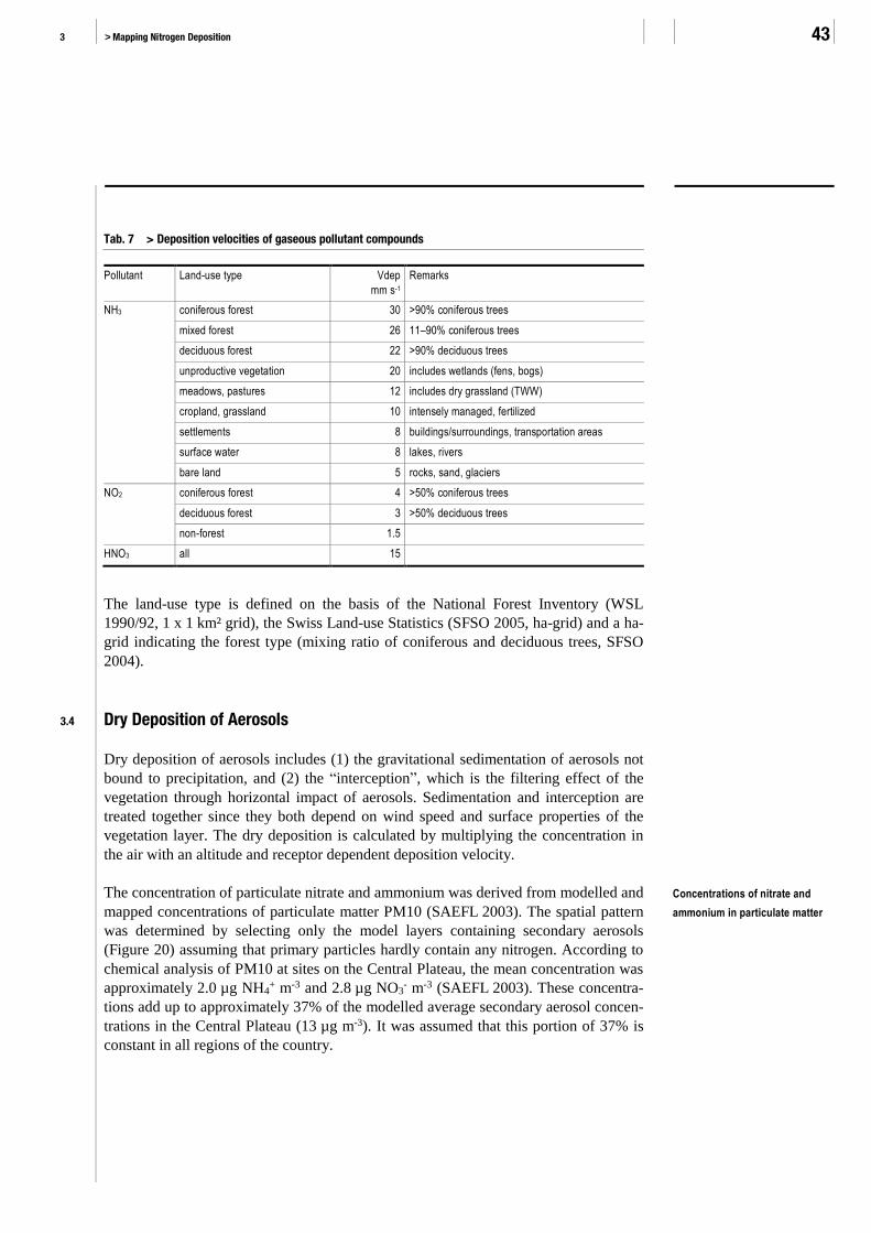
3 > Mapping Nitrogen Deposition 43
Tab. 7 > Deposition velocities of gaseous pollutant compounds
Pollutant Land-use type Vdep
mm s-1
Remarks
NH3 coniferous forest 30 >90% coniferous trees
mixed forest 26 11–90% coniferous trees
deciduous forest 22 >90% deciduous trees
unproductive vegetation 20 includes wetlands (fens, bogs)
meadows, pastures 12 includes dry grassland (TWW)
cropland, grassland 10 intensely managed, fertilized
settlements 8 buildings/surroundings, transportation areas
surface water 8 lakes, rivers
bare land 5 rocks, sand, glaciers
NO2 coniferous forest 4 >50% coniferous trees
deciduous forest 3 >50% deciduous trees
non-forest 1.5
HNO3 all 15
The land-use type is defined on the basis of the National Forest Inventory (WSL
1990/92, 1 x 1 km² grid), the Swiss Land-use Statistics (SFSO 2005, ha-grid) and a ha-
grid indicating the forest type (mixing ratio of coniferous and deciduous trees, SFSO
2004).
3.4 Dry Deposition of Aerosols
Dry deposition of aerosols includes (1) the gravitational sedimentation of aerosols not
bound to precipitation, and (2) the “interception”, which is the filtering effect of the
vegetation through horizontal impact of aerosols. Sedimentation and interception are
treated together since they both depend on wind speed and surface properties of the
vegetation layer. The dry deposition is calculated by multiplying the concentration in
the air with an altitude and receptor dependent deposition velocity.
The concentration of particulate nitrate and ammonium was derived from modelled and
mapped concentrations of particulate matter PM10 (SAEFL 2003). The spatial pattern
was determined by selecting only the model layers containing secondary aerosols
(Figure 20) assuming that primary particles hardly contain any nitrogen. According to
chemical analysis of PM10 at sites on the Central Plateau, the mean concentration was
approximately 2.0 µg NH4+ m-3 and 2.8 µg NO3
- m-3 (SAEFL 2003). These concentra-
tions add up to approximately 37% of the modelled average secondary aerosol concen-
trations in the Central Plateau (13 µg m-3). It was assumed that this portion of 37% is
constant in all regions of the country.
Concentrations of nitrate and
ammonium in particulate matter

Critical Loads of Nitrogen and their Exceedances FOEN 2016 44
Fig. 20 > Concentrations of secondary PM10, 200 x 200 m² raster
after SAEFL 2003
Vdep are average values obtained from literature (e.g. Lövblad & Erisman 1992, Asman
& van Jaarsveld 1992, Lövblad et al. 1993; Duyzer (1994), Fangmeier et al. 1994,
Hesterberg et al. 1996, Loubet et al. 2009). An estimate of the altitude dependence of
Vdep for Switzerland was observed by Riedmann & Hertz (1991) as follows (see Table
8):
Vdep(900m) = 2 • Vdep(450m)
The increase of Vdep with altitude can be explained by the fact that the average wind
speed also increases strongly, rising from 450 m to 900 m a.s.l in the Central Plateau.
Thereby the filtering effect of vegetation is reinforced. Between 900 m and 2000 m an
increase also exists, although it is smaller.
The additional filtering effect of forests is taken into account by using deposition
velocities that are 1.5–2.5 times higher than for open fields (see Table 8).
Deposition velocities of aerosols
3.6
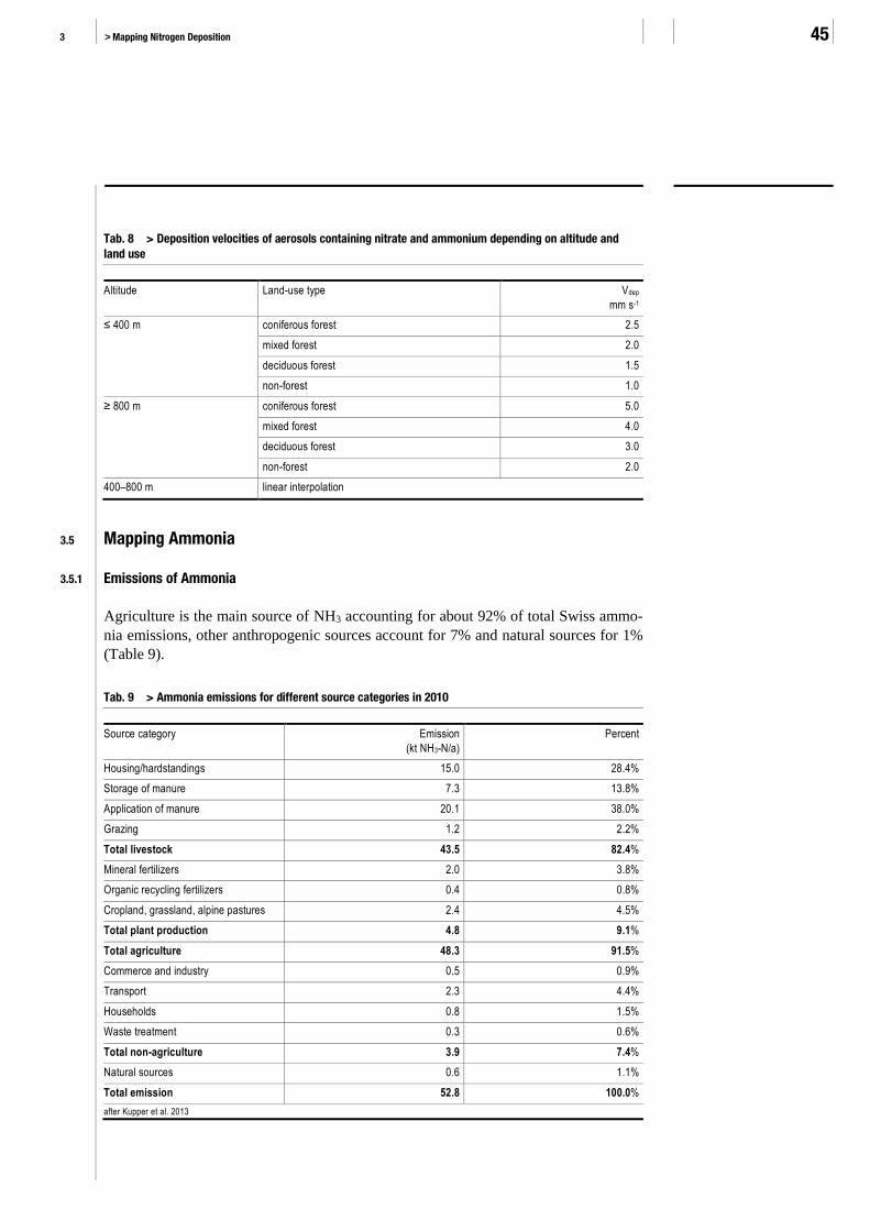
3 > Mapping Nitrogen Deposition 45
Tab. 8 > Deposition velocities of aerosols containing nitrate and ammonium depending on altitude and land use
Altitude Land-use type Vdep
mm s-1
≤ 400 m coniferous forest 2.5
mixed forest 2.0
deciduous forest 1.5
non-forest 1.0
≥ 800 m coniferous forest 5.0
mixed forest 4.0
deciduous forest 3.0
non-forest 2.0
400–800 m linear interpolation
3.5 Mapping Ammonia
3.5.1 Emissions of Ammonia
Agriculture is the main source of NH3 accounting for about 92% of total Swiss ammo-
nia emissions, other anthropogenic sources account for 7% and natural sources for 1%
(Table 9).
Tab. 9 > Ammonia emissions for different source categories in 2010
Source category Emission
(kt NH3-N/a)
Percent
Housing/hardstandings 15.0 28.4%
Storage of manure 7.3 13.8%
Application of manure 20.1 38.0%
Grazing 1.2 2.2%
Total livestock 43.5 82.4%
Mineral fertilizers 2.0 3.8%
Organic recycling fertilizers 0.4 0.8%
Cropland, grassland, alpine pastures 2.4 4.5%
Total plant production 4.8 9.1%
Total agriculture 48.3 91.5%
Commerce and industry 0.5 0.9%
Transport 2.3 4.4%
Households 0.8 1.5%
Waste treatment 0.3 0.6%
Total non-agriculture 3.9 7.4%
Natural sources 0.6 1.1%
Total emission 52.8 100.0%
after Kupper et al. 2013
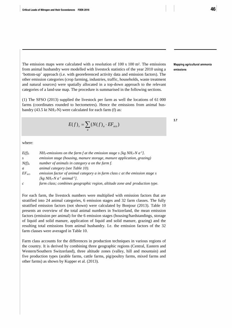
Critical Loads of Nitrogen and their Exceedances FOEN 2016 46
The emission maps were calculated with a resolution of 100 x 100 m². The emissions
from animal husbandry were modelled with livestock statistics of the year 2010 using a
‘bottom-up’ approach (i.e. with georeferenced activity data and emission factors). The
other emission categories (crop farming, industries, traffic, households, waste treatment
and natural sources) were spatially allocated in a top-down approach to the relevant
categories of a land-use map. The procedure is summarised in the following sections.
(1) The SFSO (2013) supplied the livestock per farm as well the locations of 61 000
farms (coordinates rounded to hectometres). Hence the emissions from animal hus-
bandry (43.5 kt NH3-N) were calculated for each farm (f) as:
))(()( acs
a
as EFfNfE
where:
E(f)s NH3-emissions on the farm f at the emission stage s [kg NH3-N a-1].
s emission stage (housing, manure storage, manure application, grazing)
N(f)a number of animals in category a on the farm f.
a animal category (see Table 10).
EFacs emission factor of animal category a in farm class c at the emission stage s
[kg NH3-N a-1 animal-1].
c farm class; combines geographic region, altitude zone and production type.
For each farm, the livestock numbers were multiplied with emission factors that are
stratified into 24 animal categories, 6 emission stages and 32 farm classes. The fully
stratified emission factors (not shown) were calculated by Bonjour (2013). Table 10
presents an overview of the total animal numbers in Switzerland, the mean emission
factors (emission per animal) for the 6 emission stages (housing/hardstandings, storage
of liquid and solid manure, application of liquid and solid manure, grazing) and the
resulting total emissions from animal husbandry. I.e. the emission factors of the 32
farm classes were averaged in Table 10.
Farm class accounts for the differences in production techniques in various regions of
the country. It is derived by combining three geographic regions (Central, Eastern and
Western/Southern Switzerland), three altitude zones (valley, hill and mountain) and
five production types (arable farms, cattle farms, pig/poultry farms, mixed farms and
other farms) as shown by Kupper et al. (2013).
Mapping agricultural ammonia
emissions
3.7
3 > Mapping Nitrogen Deposition 47
Tab. 10 > Emission factors, number of animals and total NH3-emissions for 24 animal categories in 2010
Emissionsfactor (kg NH3-N / a per animal)
Animal category Housing,
hard
standings
Storage
liquid
manure
Storage
solid
manure
Application
liquid
manure
Application
solid
manure
Grazing Total Number
of
animals
Emision
(kt NH3-
N/a)
Dairy cows 9.50 4.54 1.83 16.40 2.85 0.88 36.00 589 024 21.20
Suckling cows 8.87 2.60 1.50 8.15 2.59 1.29 25.00 111 291 2.78
Dairy followers
<1 yr
2.69 0.62 0.95 2.53 1.40 0.27 8.45 226 352 1.91
Dairy followers
1–2 yr
3.63 1.17 0.95 3.89 1.46 0.68 11.80 212 778 2.51
Dairy followers
>2 yr
4.76 1.50 1.36 6.44 2.20 0.84 17.10 119 163 2.04
Pre beef-
fattening calves
3.96 0.63 1.27 4.01 1.69 0.35 11.90 88 095 1.05
Beef cattle 4.21 1.29 1.42 3.76 1.84 0.07 12.60 145 084 1.83
Beef calves 1.54 0.14 1.30 0.56 1.73 0.00 5.27 99 446 0.52
Farrowing sows 10.00 2.16 0.01 4.99 0.00 - 17.20 33 508 0.58
Dry sows 6.34 1.02 0.00 2.18 0.00 0.00 9.54 106 070 1.01
Piglets <25 kg 1.11 0.21 0.02 0.54 0.00 0.00 1.89 349 206 0.66
Boars 5.56 0.89 0.04 2.07 0.00 0.02 8.58 3 685 0.03
Fattening pigs 3.17 0.48 0.00 1.67 0.00 0.00 5.33 788 149 4.20
Laying hens 0.14 - 0.04 - 0.08 0.02 0.28 2 438 051 0.68
Poultry growers 0.05 - 0.02 - 0.03 0.00 0.10 925 522 0.09
Broilers 0.06 - 0.01 - 0.06 0.00 0.12 5 580 103 0.67
Turkeys 0.18 - 0.05 - 0.14 0.01 0.38 58 074 0.02
Other poultry 0.08 - 0.04 - 0.08 0.00 0.21 23 153 0.00
Horses >3 yr 4.33 - 2.32 - 2.59 0.54 9.78 53 441 0.52
Horses <3 yr 3.70 - 1.98 - 1.95 0.71 8.33 8 672 0.07
Ponies, donkeys,
mules
1.56 - 0.73 - 1.19 0.16 3.65 20 407 0.07
Sheep 1.19 - 0.75 - 0.85 0.26 3.05 228 178 0.70
Milk sheep 2.13 - 1.00 - 1.38 0.24 4.76 12 362 0.06
Goats 1.68 - 1.11 - 1.01 0.08 3.88 54 739 0.21
Total 43.5
after Kupper et al. 2013
(2) It was assumed that the emissions from housing, hardstandings and manure storage
are located in the same hectare-cell as the farm building (total 22.3 kt NH3-N a-1, see
Tab. 9).
(3) The emissions from grazing and manure application (total 21.3 kt NH3-N a-1, see
Tab. 9) were distributed over the agricultural areas within the municipality.
Municipality boundaries are used here as a proxy for the land managed by the farms as
it is not known, on a national level, which parcels belong to a specific farm. The mu-
nicipality areas are available in digital form at swisstopo (2010). The size of the ~2800

Critical Loads of Nitrogen and their Exceedances FOEN 2016 48
municipalities varies from about 3 km² in the Plateau to more than 100 km² in alpine
regions (average 14 km²). Inside each municipality, the land use-map (SFSO 2005)
with a resolution of one hectare is used to enhance the plausibility of the spatial emis-
sion pattern. This is done by weighting the land-use categories as follows:
> Weight = 1: arable land, meadows, farm pastures, vineyards and orchards.
> Weight = 0.25: open forest (on agricultural areas), brush meadows/farm pastures,
mountain meadows and favourable alpine pastures. These categories are assumed to
emit much less ammonia than arable land and regular meadows because they are
often situated in relatively remote areas or because the season for grazing is relative-
ly short.
> Weight = 0: all other land-use categories are excluded from the area sources. Fur-
thermore, all areas protected by the Federal Inventories of Raised and Transitional
Bogs and of Fenland (see Chapter 2.2.3) are excluded as fertilizing is generally not
allowed.
(4) The portion of emissions produced by animals which spend the summer (90 days)
up on the alps amounts to 1.7 kt NH3-N. On the one hand, this emission quantity was
subtracted from the emissions of the respective farms (with municipalities as spatial
reference). On the other hand, these emissions were redistributed over the land-use
type “alpine pastures” for the whole of Switzerland. The portion of summered animals
was calculated from livestock statistics 2000 (SFSO 2013).
(5) Emissions from the application of mineral fertilizer and organic recycling fertilizer
(total 2.4 kt NH3-N a-1, see Tab. 9) were distributed over the land-use categories arable
land, meadows, farm pastures, vineyards and orchards.
(6) Emissions on agricultural land arising from processes in the plant layer (total 2.4 kt
NH3-N a-1, see Tab. 9) were allocated according to Kupper et al. (2013):
> An emission factor of 2.0 kg NH3-N ha-1 was applied on land-use categories arable
land, meadows, farm pastures, vineyards and orchards. The total area is 1 060 kha
and the resulting emission is 2.1 kt NH3-N a-1.
> An emission factor of 0.5 kg NH3-N ha-1 was applied on land-use categories moun-
tain meadows, favourable alpine pastures, remote/steep alpine meadows and re-
mote/steep alpine pastures. The total area is 538 kha and the resulting emission is
0.3 kt NH3-N a-1.
(7) Emissions from commerce and industry (0.5 kt NH3-N a-1) were distributed over
the land-use categories industrial buildings and industrial grounds.
(8) The ammonia emissions from transport were mapped by a bottom-up approach for
the year 2000. It was based on a traffic model including the main road-networks and
zonal traffic (SAEFL 2004). This emission map was proportionally rescaled to the total
transport emission in 2010 (2.3 kt NH3-N a-1).
(9) Emissions from households (0.8 kt NH3-N a-1) were distributed over the land-use
categories residential areas, agricultural buildings and garden allotments.
Ammonia emissions from
industry, commerce, traffic,
households and waste treatment

3 > Mapping Nitrogen Deposition 49
(10) Emissions from treatment of waste-water and solid waste (0.3 kt NH3-N a-1) were
distributed over the land-use categories ‘waste water treatment plants’ and dumps.
(11) Natural emissions (0.6 kt NH3-N a-1) originating from soil processes on natural
grassland as well as from wild animals were distributed over the land-use categories
forests, woods and unproductive grass/shrubs.
The resulting emission map is shown in Figure 24.
Fig. 21 > Ammonia emissions 2010, modelled on 100 x 100 m² raster
Resolution displayed on map: 1 x 1 km².
Natural ammonia emissions
Critical Loads of Nitrogen and their Exceedances FOEN 2016 50
3.5.2 Ammonia Concentration
A statistical dispersion model with a resolution of 100 x 100 m² was applied to calcu-
late annual mean concentrations of ammonia in the air. It includes all emission sources
at a maximum distance of 50 km. For each raster-cell the concentration C (µg m−3)
induced by the emissions from surrounding sources was calculated as:
))(14/17( i
i
i DpEC
where:
i denotes all sources (raster-cells) within a radius of 50 km.
Ei NH3-emission from raster-cell i (kg NH3-N a-1), see Chapter 3.5.2.
17/14 conversion from [kg NH3-N] to [kg NH3].
Di Distance to source i (m).
p(Di) average dispersion-profile; concentration as a function of Di.
p(D) is a normalised average distance-function providing the annual mean concentra-
tion (µg m−3) induced by one kg NH3 a-1 emitted from a source at a distance of D (see
Figure 22 and Annex). The function was calculated by Asman & Jaarsveld (1990)
using an atmospheric transport model. The model was applied and tested in several
countries (The Netherlands, United Kingdom, Belgium, Denmark and Sweden) and in
Europe (Asman & Jaarsveld 1992). In Switzerland, the integrated distance-function
shown in Figure 22 and Equation 3.8 was used the first time by Rihm & Kurz (2001) to
calculate NH3-concentration maps; the comparison with measured NH3-concentrations
was promisingly good. Thus, the method was further developed and used for mapping
NH3 in Switzerland by Thöni et al. (2005), Rihm et al. (2009) and EKL (2014).
The function p(D) integrates effects of several atmospheric processes such as dilution
by turbulence, deposition on the ground and chemical transformation of ammonia to
ammonium. It is related to a point source at a height of 3 m above ground and the
resulting concentrations are given for a reference height of 1 m above ground. In the
present study, it was assumed that the sources and the receptor points are situated in the
centre of the 100 x 100 m² cells. For calculating the concentration in a raster-cell
induced by the emission of the same cell (where D = 0 m), a distance of 50 m was used
in p(D).
Mapping ammonia concentrations
3.8

3 > Mapping Nitrogen Deposition 51
Fig. 22 > NH3 concentration as a function of the distance to a source emitting 1 kg NH3 a-1 for distances between 50 m and 50 km
See Annex.
by Asman & Jaarsveld 1990
In this study, the calculation was made with a resolution of 100 x 100 m² for distances
below 4 km. Due to computing performance, distances between 4 km and 50 km were
calculated on the basis of spatially aggregated emission-data with a resolution of
1 x 1 km².
Furthermore, two different climatic regions were defined for the calculation of distanc-
es below 4 km:
> In the first region (covering the Alps and Southern Switzerland), the function p(D)
was applied rotation-symmetrically (Figure 23, left).
> In the second region (covering the Jura Mountains and the Swiss Plateau) the p(D)
function was modified according to prevailing wind directions in this area (Figure
23, right); i.e. the concentration is calculated as a function of distance and azimuth
between source and receptor. The modification was based on the region-specific
dispersion profiles developed for NO2 (FOEN 2011).
The resulting map of ammonia concentrations in 2010 is shown in Figure 24.
1.0E-09
1.0E-08
1.0E-07
1.0E-06
1.0E-05
1.0E-04
1.0E-03
1.0E-02
10 100 1'000 10'000
NH
3co
nce
ntr
atio
n (
µg
m-3
)
Distance (m)

Critical Loads of Nitrogen and their Exceedances FOEN 2016 52
Fig. 23 > Schematic dispersion profiles for distances 50–4000 m
Rotation-symmetric use of p(D) in the Alps and Southern Switzerland.
Modified p(D) function according to prevailing wind directions in the Jura/Plateau region.
Fig. 24 > Map of NH3 concentration in 2010, 100 x 100 m² raster
3.5.3 Validation of the Ammonia Maps
The modelled concentrations can be validated by comparing with measurements pro-
vided by Seitler & Thöni (2016). These measurements show that there is an inter-
annual variation of concentrations due to climate (higher concentrations in warm years)
but there is no significant trend between 2000 and 2014. For the comparison shown in
Figure 25, 48 monitoring sites with complete time-series 2008–2012 were selected and
the average of the 5-year period was used as the modelled values do not include climat-
ic variations.
Comparison of modelled and
measured ammonia
concentrations
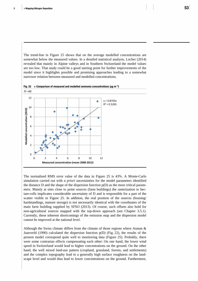
3 > Mapping Nitrogen Deposition 53
The trend-line in Figure 25 shows that on the average modelled concentrations are
somewhat below the measured values. In a detailed statistical analysis, Locher (2014)
revealed that mainly in Alpine valleys and in Southern Switzerland the model values
are too low. That study could be a good starting point for further improvements of the
model since it highlights possible and promising approaches leading to a somewhat
narrower relation between measured and modelled concentrations.
Fig. 25 > Comparison of measured and modelled ammonia concentrations (µg m−3)
N=48.
The normalised RMS error value of the data in Figure 25 is 43%. A Monte-Carlo
simulation carried out with a priori uncertainties for the model parameters identified
the distance D and the shape of the dispersion function p(D) as the most critical param-
eters. Mainly at sites close to point sources (farm buildings) the rasterization to hec-
tare-cells implicates considerable uncertainty of D and is responsible for a part of the
scatter visible in Figure 25. In addition, the real position of the sources (housing/
hardstandings, manure storage) is not necessarily identical with the coordinates of the
main farm building supplied by SFSO (2013). Of course, such offsets also hold for
non-agricultural sources mapped with the top-down approach (see Chapter 3.5.1).
Currently, these inherent shortcomings of the emission map and the dispersion model
cannot be improved at the national level.
Although the Swiss climate differs from the climate of those regions where Asman &
Jaarsveld (1990) calculated the dispersion function p(D) (Fig. 22), the results of the
present model correspond quite well to monitoring data (Figure 25). Probably, there
were some contrarian effects compensating each other: On one hand, the lower wind
speed in Switzerland would lead to higher concentrations on the ground. On the other
hand, the well mixed land-use pattern (cropland, grassland, forests, and settlements)
and the complex topography lead to a generally high surface roughness on the land-
scape level and would thus lead to lower concentrations on the ground. Furthermore,
y = 0.8703xR² = 0.5265
0
2
4
6
8
10
12
0 2 4 6 8 10 12
Mo
de
lled
co
nce
ntr
atio
n (
20
10
)
Measured concentration (mean 2008-2012)
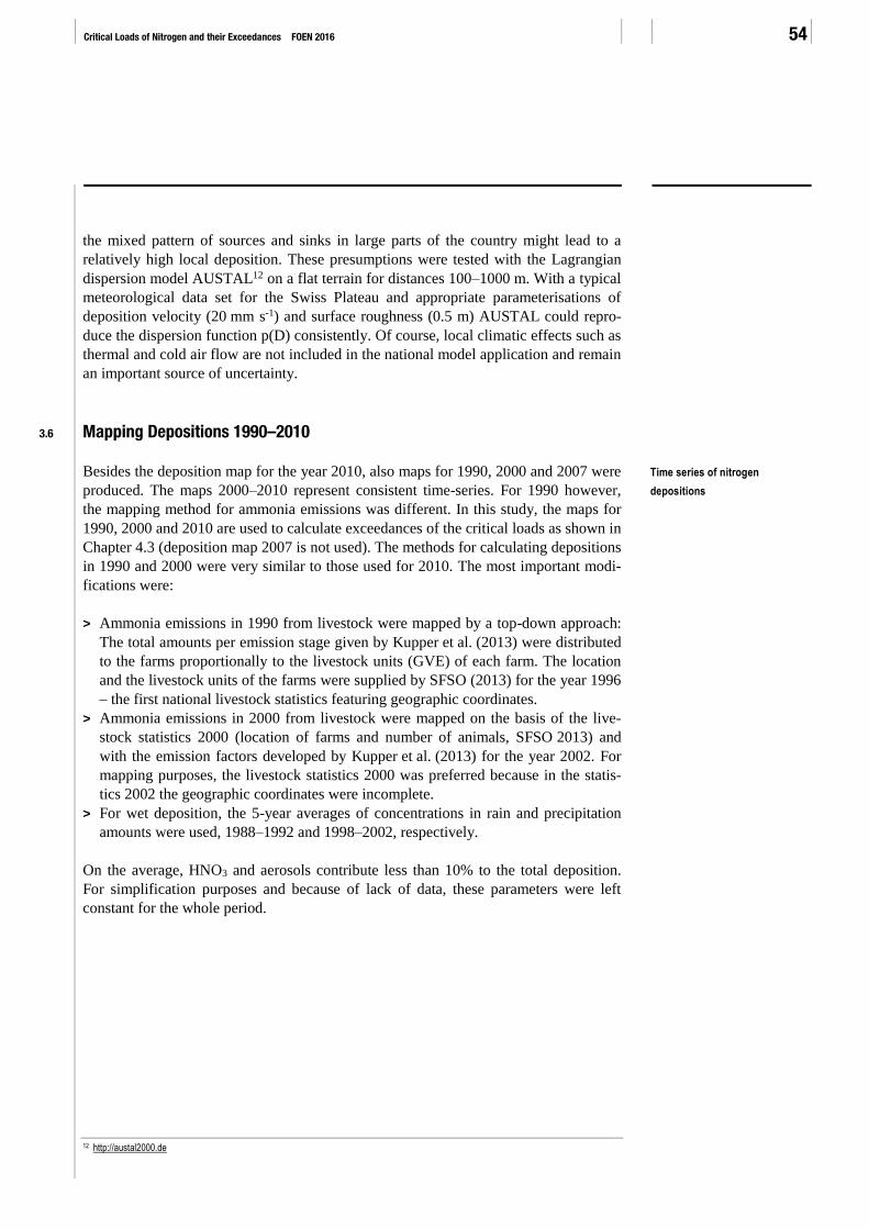
Critical Loads of Nitrogen and their Exceedances FOEN 2016 54
the mixed pattern of sources and sinks in large parts of the country might lead to a
relatively high local deposition. These presumptions were tested with the Lagrangian
dispersion model AUSTAL12 on a flat terrain for distances 100–1000 m. With a typical
meteorological data set for the Swiss Plateau and appropriate parameterisations of
deposition velocity (20 mm s-1) and surface roughness (0.5 m) AUSTAL could repro-
duce the dispersion function p(D) consistently. Of course, local climatic effects such as
thermal and cold air flow are not included in the national model application and remain
an important source of uncertainty.
3.6 Mapping Depositions 1990–2010
Besides the deposition map for the year 2010, also maps for 1990, 2000 and 2007 were
produced. The maps 2000–2010 represent consistent time-series. For 1990 however,
the mapping method for ammonia emissions was different. In this study, the maps for
1990, 2000 and 2010 are used to calculate exceedances of the critical loads as shown in
Chapter 4.3 (deposition map 2007 is not used). The methods for calculating depositions
in 1990 and 2000 were very similar to those used for 2010. The most important modi-
fications were:
> Ammonia emissions in 1990 from livestock were mapped by a top-down approach:
The total amounts per emission stage given by Kupper et al. (2013) were distributed
to the farms proportionally to the livestock units (GVE) of each farm. The location
and the livestock units of the farms were supplied by SFSO (2013) for the year 1996
– the first national livestock statistics featuring geographic coordinates.
> Ammonia emissions in 2000 from livestock were mapped on the basis of the live-
stock statistics 2000 (location of farms and number of animals, SFSO 2013) and
with the emission factors developed by Kupper et al. (2013) for the year 2002. For
mapping purposes, the livestock statistics 2000 was preferred because in the statis-
tics 2002 the geographic coordinates were incomplete.
> For wet deposition, the 5-year averages of concentrations in rain and precipitation
amounts were used, 1988–1992 and 1998–2002, respectively.
On the average, HNO3 and aerosols contribute less than 10% to the total deposition.
For simplification purposes and because of lack of data, these parameters were left
constant for the whole period.
12 http://austal2000.de
Time series of nitrogen
depositions
4 > Results 55
4 > Results - - - - - - - - - - - - - - - - - - - - - - - - - - - - - - - - - - - - - - - - - - - - - - - - - - - - - - - - - - - - - - - - - - - - - - - - - - - - - - - - - - - - - - - - - - - - - - - - - - - - - - - - - - - - - - -
4.1 Critical Loads of Nitrogen
The spatial distributions of critical loads are displayed separately for the empirical
method and for the SMB method on the maps in Figure 26 and Figure 27, respectively.
The map in Figure 26 is a combination of all selected ecosystems as described in
chapter 2.2.3. Only (semi-)natural ecosystems with high conservation importance were
included. For each cell of the 1 x 1 km² raster, the critical load value of the most sensi-
tive ecosystem existing in the cell was selected. The map in Figure 28 combines the
results of the empirical method and SMB method showing the minimum critical load of
both.
Figure 29 presents the critical loads as cumulative frequency distributions.
Fig. 26 > Empirical critical loads of nutrient nitrogen for (semi-)natural ecosystems, CLemp(N)

Critical Loads of Nitrogen and their Exceedances FOEN 2016 56
Fig. 27 > Critical loads of nutrient nitrogen for forests, CLnut(N)
Fig. 28 > Combined critical loads of nutrient nitrogen, minimum of CLnut(N) and CLemp(N) per km²

4 > Results 57
Fig. 29 > Cumulative frequency distributions of critical loads of nutrient nitrogen for Switzerland
The SMB method was applied to forests, the empirical method to (semi-)natural ecosystems.
The critical loads for natural and semi-natural ecosystems (CLemp[N]), empirical meth-
od, chapter 2.2) are in the range from 4 to 15 kg N ha-1 a-1 covering a total sensitive
area of 18 584 km². The most sensitive ecosystems are alpine lakes, raised bogs, Litto-
rellion, (sub-)alpine scrub habitats and (sub-)alpine grassland (4–10 kg N kg N ha-1a-1).
The largest part of these sensitive areas is covered by (sub-)alpine grassland and scrub
habitats; these poorly managed pastures and meadows represent a very important part
of the Alpine vegetation. Because of their short vegetation period, the low temperatures
and the relatively poor soils, their natural nitrogen demand, and consequently their
critical load, is low. Critical load between 10 and 15 kg N ha-1 a-1 were assigned to
selected species-rich montane and sub-alpine grassland, fens and poorly managed
forests with especially rich ground-flora.
In the Swiss Plateau, between the Alps and the Jura mountains, relatively few sensitive
areas can be found on Figure 26. This can be explained by the fact that in this region a
large part of the (semi-)natural ecosystems has disappeared, mainly due to intense
agricultural management (e.g. mountain hay meadows, see Bosshard 2015). Two main
reasons can be mentioned for the poor occurrence of (semi-)natural ecosystems in the
Central and Southern Alps: (1) Acidic alpine grasslands such as caricion curvulae /
sempervirentis and nardion have not been included, and (2) large areas south of the
Alps are covered by forest, which was included in the SMB method.
The critical loads for productive and managed forests (CLnut(N), calculated with the
SMB method (see chapter 2.3) are in the range from 10 to 25 kg N ha-1 a-1 covering a
total sensitive area of 10 632 km² (Fig. 27). As described in Chapter 2.3.1, the lower
range of 10 kg N ha-1 a-1 was set with intent to avoid implausible low values. The
variation of the critical loads is mainly due to the removal of nitrogen by harvesting
and denitrification losses. The average harvesting rates in the mountainous regions and
south of the Alps are lower than in the Plateau (Fig. 12). The denitrification rates
depend on the percolation conditions of the soils. The highest denitrification rates and
0
10
20
30
40
50
60
70
80
90
100
0 2 4 6 8 10 12 14 16 18 20
[%]
[kg N ha-1 a-1]
CLemp(N), empirical
CLnut(N), SMB
Critical loads of nitrogen for
(semi-)natural ecosystems
Critical loads of nitrogen for
forests
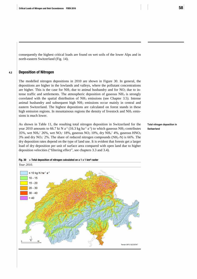
Critical Loads of Nitrogen and their Exceedances FOEN 2016 58
consequently the highest critical loads are found on wet soils of the lower Alps and in
north-eastern Switzerland (Fig. 14).
4.2 Deposition of Nitrogen
The modelled nitrogen depositions in 2010 are shown in Figure 30. In general, the
depositions are higher in the lowlands and valleys, where the pollutant concentrations
are higher. This is the case for NH3 due to animal husbandry and for NO2 due to in-
tense traffic and settlements. The atmospheric deposition of gaseous NH3 is strongly
correlated with the spatial distribution of NH3 emissions (see Chapter 3.5). Intense
animal husbandry and subsequent high NH3 emissions occur mainly in central and
eastern Switzerland. The highest depositions are calculated on forest stands in these
high emission regions. In mountainous regions the density of livestock and NH3 emis-
sions is much lower.
As shown in Table 11, the resulting total nitrogen deposition in Switzerland for the
year 2010 amounts to 66.7 kt N a-1 (16.3 kg ha-1 a-1) to which gaseous NH3 contributes
35%, wet NH4+ 26%, wet NO3
- 18%, gaseous NO2 10%, dry NH4+ 4%, gaseous HNO3
3% and dry NO3- 2%. The share of reduced nitrogen compounds (NHy-N) is 66%. The
dry deposition rates depend on the type of land use. It is evident that forests get a larger
load of dry deposition per unit of surface area compared with open land due to higher
deposition velocities (“filtering effect”, see chapters 3.3 and 3.4).
Fig. 30 > Total deposition of nitrogen calculated on a 1 x 1 km² raster
Year 2010.
Total nitrogen deposition in
Switzerland

4 > Results 59
Tab. 11 > Total deposition of N compounds in Switzerland
Year 2010. Units: kt N a-1 (italic: kg N ha-1 a-1).
Receptors Compounds Forest
11 366 km²
Non-forest
29 683 km²
Total
41 049 km²
Wet NH4+ 5.6 5.0 12.0 4.1 17.7 4.3
Dry
NH4+ aerosol 1.4 1.2 1.5 0.5 2.9 0.7
NH3 gas 10.1 8.9 13.5 4.6 23.6 5.8
Total NHy-N 17.2 15.1 27.1 9.1 44.2 10.8
Wet NO3- 4.0 3.5 8.3 2.8 12.3 3.0
Dry
NO3- aerosol 0.6 0.5 0.6 0.2 1.2 0.3
NO2 gas 3.4 3.0 3.5 1.2 6.9 1.7
HNO3 gas 0.6 0.5 1.5 0.5 2.1 0.5
Total NOy-N 8.6 7.6 13.9 4.7 22.5 5.5
Total N 25.8 22.7 41.0 13.8 66.7 16.3
The values in Table 11 can be compared with the independent results of the European
EMEP-Model. EMEP applies an atmospheric transport model to the national emission
data, resulting in a country-to-country transfer and deposition matrix with a spatial
resolution of 50 x 50 km². The modelled total deposition for Switzerland in 2010 was
62 kt a-1 (Gauss et al. 2015), i.e. the difference is only -8%. Another independent
model result was provided by Aksoyoglu (2014): She calculated dry N depositions in
2006 with the CAMx13 model (raster size ~4 x 6 km²); the resulting total dry deposition
for Switzerland was 32.7 kt N a-1 (difference -11%) and the gas deposition of NH3 was
23.7 kt N a-1 (difference +0.2%).
An independent deposition study at a single site is available from 1992/1993: Neftel &
Wanner (1994) carried out comprehensive field measurements on a meadow at Meren-
schwand (rural area of the Swiss Central Plateau) and found a total N deposition of 27–
30 kg N ha-1 a-1 (depending on the measurement method for NH3). This is in agreement
with the temporally interpolated result of the deposition models 1990 and 2000 for the
same site (28 kg N ha-1 a-1).
The modelled depositions were also compared with throughfall measurements in
forests (e.g. Thimonier et al. 2005). Generally, the total depositions derived from
throughfall were lower than the modelled depositions. There are several possible
reasons for this: (1) The model does not incorporate forest edge effects, which may
overestimate dry nitrogen deposition at inner parts of forest areas, where the measure-
ment sites are situated in general. (2) The N depositions derived from throughfall may
underestimate direct canopy uptake of N. (3) Omitting stemflow in the measurements
leads to underestimations of deposition. (4) At higher altitudes, snowfall can contribute
to the underestimation of precipitation measurements. As mentioned in chapter 3.2,
various parameters were adapted in the current model based on the study by Thi-
monier et al. (2005).
13 www.camx.com
Nitrogen depositions resulting
from different modelling
approaches

Critical Loads of Nitrogen and their Exceedances FOEN 2016 60
From 1990 to 2010 the total deposition in Switzerland was reduced by 23% (Table 12).
14% of this reduction took place between 1990 and 2000, i.e. the change was less
pronounced since 2000, especially for the gaseous deposition of ammonia. This is in
accordance with measured ammonia concentrations, which show no significant trend
between 2000 and 2014 (Seitler & Thöni 2015). HNO3 and aerosols contribute less
than 10% to the total deposition. For simplification purposes and because of lack of
data aerosols were left constant for the whole period; maps of HNO3 were available for
the years 1990 and 2000 and the latter was also used for 2010.
Tab. 12 > Total deposition von N compounds in Switzerland
Years 1990, 2000 and 2010. Units: kt N a-1.
Compounds
1990 2000 2010
Wet NH4+ 24.9 21.4 17.7
Dry
NH4+ aerosol 2.9 2.9 2.9
NH3 gas 26.9 23.9 23.6
Total NHy-N 54.7 48.3 44.2
Wet NO3- 18.9 14.9 12.3
Dry
NO3- aerosol 1.2 1.2 1.2
NO2 gas 9.2 7.6 6.9
HNO3 gas 2.4 2.1 2.1
Total NOy-N 31.7 25.8 22.5
Total N 86.4 74.1 66.7
Total N, percent 100% 86% 77%
4.3 Exceedances of Critical Loads of Nitrogen
Exceedances are calculated as deposition minus critical load. Thus, a negative exceed-
ance means “not exceeded”. Exceedance of critical loads indicates a long-term risk of
adverse effects in the ecosystems (see chapter 2.1) due to increased nitrogen deposi-
tion.
The spatial distributions of the exceedances of critical loads are displayed in Figure 31
([semi-]natural ecosystems, empirical critical loads) and Figure 32 (forest, SMB meth-
od). The map in Figure 31 shows the exceedance of the most sensitive ecosystem type
occurring in each 1 x 1 km² raster cell, i.e. the maximum exceedance.
The map in Figure 33 combines the exceedance of the critical loads for (semi-)natural
ecosystems and forests showing the maximum exceedance per km².
Spatial distribution of
exceedances of critical loads
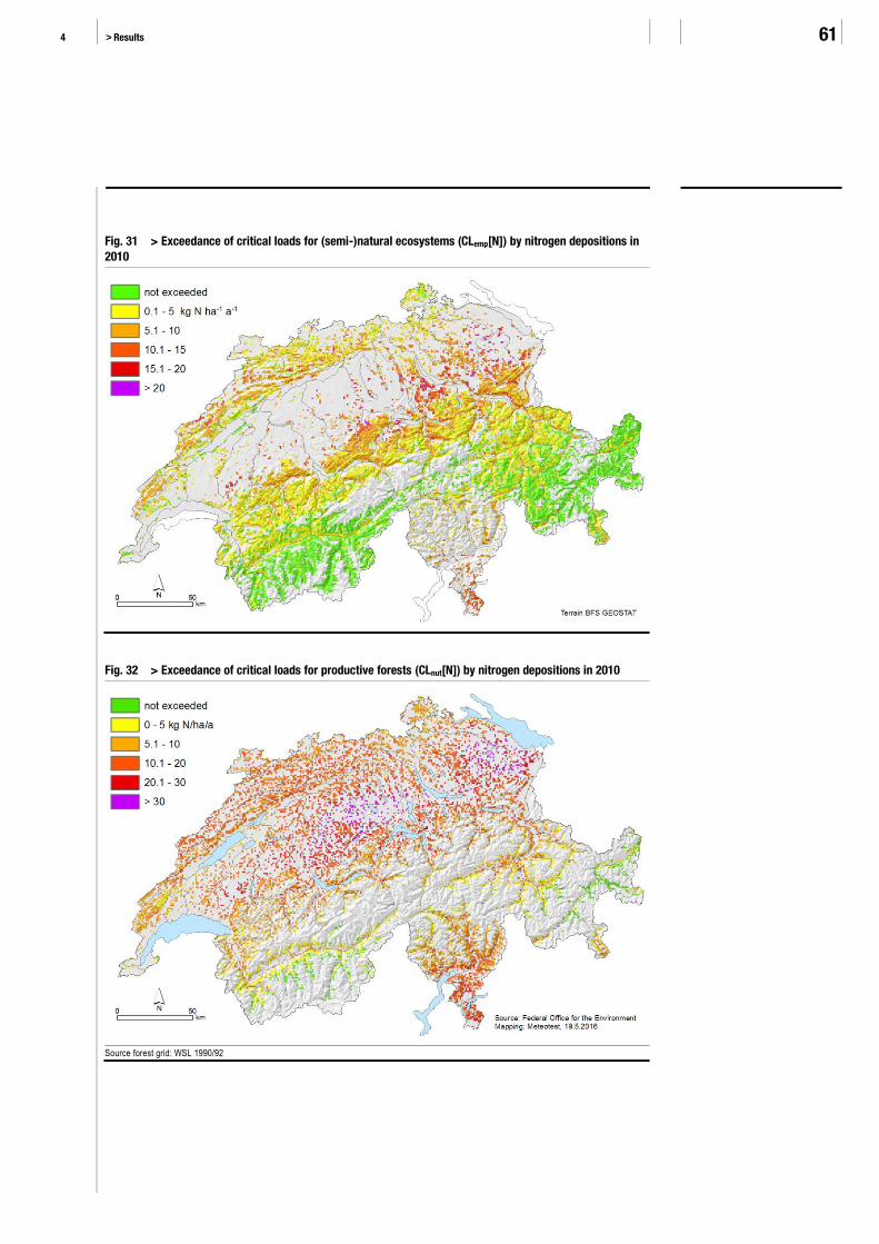
4 > Results 61
Fig. 31 > Exceedance of critical loads for (semi-)natural ecosystems (CLemp[N]) by nitrogen depositions in 2010
Fig. 32 > Exceedance of critical loads for productive forests (CLnut[N]) by nitrogen depositions in 2010
Source forest grid: WSL 1990/92
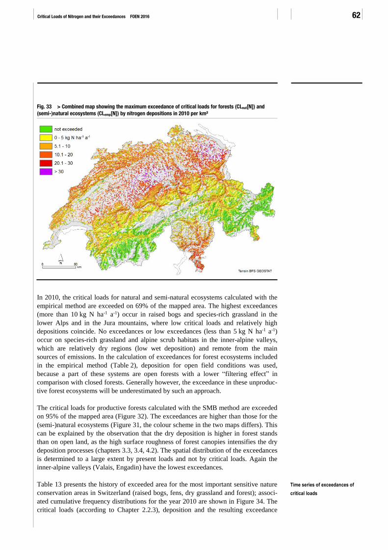
Critical Loads of Nitrogen and their Exceedances FOEN 2016 62
Fig. 33 > Combined map showing the maximum exceedance of critical loads for forests (CLnut[N]) and (semi-)natural ecosystems (CLemp[N]) by nitrogen depositions in 2010 per km²
In 2010, the critical loads for natural and semi-natural ecosystems calculated with the
empirical method are exceeded on 69% of the mapped area. The highest exceedances
(more than 10 kg N ha-1 a-1) occur in raised bogs and species-rich grassland in the
lower Alps and in the Jura mountains, where low critical loads and relatively high
depositions coincide. No exceedances or low exceedances (less than 5 kg N ha-1 a-1)
occur on species-rich grassland and alpine scrub habitats in the inner-alpine valleys,
which are relatively dry regions (low wet deposition) and remote from the main
sources of emissions. In the calculation of exceedances for forest ecosystems included
in the empirical method (Table 2), deposition for open field conditions was used,
because a part of these systems are open forests with a lower “filtering effect” in
comparison with closed forests. Generally however, the exceedance in these unproduc-
tive forest ecosystems will be underestimated by such an approach.
The critical loads for productive forests calculated with the SMB method are exceeded
on 95% of the mapped area (Figure 32). The exceedances are higher than those for the
(semi-)natural ecosystems (Figure 31, the colour scheme in the two maps differs). This
can be explained by the observation that the dry deposition is higher in forest stands
than on open land, as the high surface roughness of forest canopies intensifies the dry
deposition processes (chapters 3.3, 3.4, 4.2). The spatial distribution of the exceedances
is determined to a large extent by present loads and not by critical loads. Again the
inner-alpine valleys (Valais, Engadin) have the lowest exceedances.
Table 13 presents the history of exceeded area for the most important sensitive nature
conservation areas in Switzerland (raised bogs, fens, dry grassland and forest); associ-
ated cumulative frequency distributions for the year 2010 are shown in Figure 34. The
critical loads (according to Chapter 2.2.3), deposition and the resulting exceedance
Time series of exceedances of
critical loads

4 > Results 63
were calculated on a 100 x 100 m² raster (cf. EKL 2014). For forests, the exceedance
was calculated on the 1 x 1 km² sampling points of the national forest inventory as
shown in Figure 32 (WSL 1990/92). For all these ecosystems a reduction of the ex-
ceeded area can be observed between 1990 and 2000 which continues between 2000
and 2010. However the percentage of exceeded area remains very high. The lowest
exceedance was calculated for dry grassland (TWW) as these conservation areas are
generally situated in dry regions and remote from strong sources of nitrogen emissions.
Tab. 13 > Exceedance of critical loads of nutrient nitrogen for different protected ecosystems in Switzerland in 1990, 2000 and 2010
Units: percent of total ecosystem area.
Ecosystem Area
km²
1990 2000 2010
Raised bogs 52 100 100 98
Fens 188 91 82 76
Dry grassland (TWW) 200 81 62 49
Forest 10 290 99 96 95
Fig. 34 > Cumulative frequency distribution of the exceedances of critical loads of nutrient nitrogen for different protected ecosystems
Units: percent of total ecosystem area. Nitrogen deposition: year 2010.
The exceedances of critical loads shown in this Chapter indicate a risk of adverse
effects in the long-term. Actually, harmful effects of excess nitrogen deposition were
shown in various studies in Switzerland. E.g. for the raised bogs and fens, Klaus (2007)
observed a declining quality of the ecosystem areas between surveys in 1997/2001 and
2002/2006, especially also an increase in nutrient availability. For beech forests, a clear
decrease of root mycorrhiza with increasing N deposition was found (de Witte et al.
0%
10%
20%
30%
40%
50%
60%
70%
80%
90%
100%
0 5 10 15 20 25 30
Pe
rce
nt o
f to
tal e
co
syste
m a
rea
Exceedance (kg N ha-1 a-1)
Raised bogs
Fens
Dry grassland (TWW)
Forest
Adverse effects of exceedances
of critical loads

Critical Loads of Nitrogen and their Exceedances FOEN 2016 64
2015). Roth et al. (2013 and 2017) showed significant relations between the increase of
N-deposition and decrease of species richness in mountain hay meadows and in (sub-)
alpine scrub habitats (see also chapter 2.2.2) and Roth et al. (2015) detected negative
relationships of N deposition and various biodiversity measures at the landscape scale.
4.4 Reliability of the Results
Uncertainties in the computation of critical loads and depositions involve associated
uncertainty in the exceedance of critical loads. It is a challenging task to quantify that
uncertainty as the relevant processes take place in open, interacting (eco)systems. As
explicated by de Vries et al. (2015, chapter 25), the critical load approach meets pre-
cautionary principles to support environmental sustainability; it aims at “preventing
damage caused by deposition even when scientific proof would not be conclusive”.
However, for supporting air pollution policies, information about the reliability of the
critical load exceedances is needed. Therefore, a straight-forward sensitivity analysis
was carried out and is presented in this chapter.
For empirical critical loads, the range of CLemp(N) given in the mapping manual par-
tially reflects the uncertainty of the critical load (see chapter 2.2.1). E.g. for deciduous
woodland the range is 10–20 kg N ha-1 a-1. Thus, assuming a critical load value of
15 kg N ha-1 a-1, the range corresponds to an uncertainty of approximately ±30%.
Uncertainty assessments of critical loads calculated with the SMB method (CLSMB[N])
are quite rare (de Vries et al. 2015, chapter 25). For this sensitivity analysis the same
uncertainty as for CLemp(N) is used (±30%). This assumption is also supported by a
former sensitivity analysis of FOEFL (1996) where the influence of single input pa-
rameters to the SMB was analysed.
The error of modelled depositions can be quite large, e.g. for ammonia concentrations
an error of 43% was calculated (chapter 3.5.3). However, the influence of these uncer-
tainties on the reliability of the exceedance is limited when moving from site-specific
calculations to regional applications as it was done here for the Swiss territory: As
mentioned in chapter 4.2, the comparison of the sum of N deposition in Switzerland
with two independent model results showed deviations of 8% (total deposition) and
11% (dry deposition).
Keeping these uncertainty ranges in mind, the following scenarios were defined in the
sensitivity analysis:
> Standard run: These are the results presented in chapter 4.3 for the year 2010; those
maps are considered as “best available” maps reflecting the current state of
knowledge.
> CLN+30: All critical load values are increased by 30%.
> CLN-30: All critical load values are decreased by 30%.
> Dep-30: All deposition values are decreased by 30%.
> Dep+30: All deposition values are increased by 30%.
Sensitivity analysis

4 > Results 65
The outcome of the sensitivity analysis (expressed as percentage of exceeded ecosys-
tem area) is shown in Table 14: For raised bogs and forests, the range of the exceed-
ances is quite narrow in all scenarios (79%–100%), i.e. the magnitude of the exceed-
ance is generally higher than the supposed uncertainties and therefore the reliability of
the exceedance maps is very high. The range for dry grassland (TWW) is much wider
(18%–83%), i.e. the prediction of exceedances is less reliable for this ecosystem.
Nevertheless, a relevant part of the protected dry grasslands still exhibits an exceed-
ance in scenario Dep-30 (minus 30% deposition). For fens, the range of exceedance is
in-between (35%–92%).
Tab. 14 > Exceedance of critical loads of nutrient nitrogen for the standard run and four scenarios of the sensitivity analysis
Units: percent of total ecosystem area.
Ecosystem CLN
+30%
Standard 2010 CLN
-30%
Raised bogs 92% 98% 100%
Fens 49% 76% 92%
Dry grassland (TWW) 26% 49% 83%
Forest 85% 95% 99%
Ecosystem Deposition
-30%
Standard 2010 Deposition
+30%
Raised bogs 91% 98% 100%
Fens 35% 76% 90%
Dry grassland (TWW) 18% 49% 78%
Forest 79% 95% 98%
Critical Loads of Nitrogen and their Exceedances FOEN 2016 66
5 > Conclusions - - - - - - - - - - - - - - - - - - - - - - - - - - - - - - - - - - - - - - - - - - - - - - - - - - - - - - - - - - - - - - - - - - - - - - - - - - - - - - - - - - - - - - - - - - - - - - - - - - - - - - - - - - - - - - -
This report provides an overall view of important aspects of the eutrophication problem
in Switzerland. Maps of critical loads of nitrogen and of areas where they are exceeded
were produced for whole Switzerland by combining data on the sensitivity of ecosys-
tems and on atmospheric N deposition, consequently applying the critical load concept
and the mapping methods proposed by the ICP Modelling & Mapping under the
UNECE Convention on Long-range Transboundary Air Pollution (UNECE 2016).
Since the last national report on critical loads (FOEFL 1996) the reliability of critical
loads and modelled nitrogen depositions and critical load exceedances was improved,
mainly by refining definitions and values of empirical critical loads under the Conven-
tion, by deriving country-specific critical loads based on Swiss biodiversity data, by
enhancing the resolution of the deposition model and by improving the ammonia
dispersion model.
The present atmospheric deposition of nitrogen in most forest sites and in many natural
and semi-natural ecosystems in Switzerland exceeds the critical load with respect to
eutrophication criteria. This means that the present nitrogen depositions do not meet
the target of sustainability in large areas of Switzerland, as they are beyond the ecolog-
ically safe limit, above which adverse effects must be expected in the long-term. The
situation is less severe for (sub-)alpine grassland, alpine scrub habitats and forests in
the inner-alpine valleys (Valais, Grisons), where the critical loads are not exceeded or
where the exceedances are relatively small.
While these conclusions can be drawn from the results of the study presented here, they
are also supported by various studies based on field observations and experiments,
especially concerning adverse effects on biodiversity and tree health. It is important to
note that the natural deposition is estimated to be around 1–2 kg N ha-1 a-1 (Par-
do et al. 2011, Bertills & Näsholm 2000, Binkley & Högberg 1997). Today such values
can only be observed in very remote areas, e.g. northern Scandinavia.
This means that, as a consequence of anthropogenic emissions of nitrogen compounds,
present loads of nitrogen in Switzerland are almost one order of magnitude higher than
the natural nitrogen deposition. They range from 3 kg N ha-1 a-1 (1 percentile) to 44 kg
N ha-1 a-1 (99 percentile) with an overall average of 16 kg N ha-1 a-1.
In the long-term, the exceedances of critical loads indicate potential risks for forests
such as changes in nutrient conditions, growth disturbances (unbalanced root/shoot
ratios), increased susceptibility to gales, frost, drought, insect pests and pathogens, loss
of stability and decreased biodiversity of the ground flora. For (semi-)natural ecosys-
tems, exceedances indicate a potential risk for changes in competitive relationships
between species, resulting in loss of biodiversity. The critical load approach does not
allow quantifying those risks precisely, but one can say that they are potentially more
severe the higher the exceedance is and the longer it lasts.
5 > Conclusions 67
In order to improve the situation it is necessary to further reduce the emissions of air
pollutants from agricultural activities (NH3) and from combustion processes (NOx). As
the transboundary fluxes of nitrogen compounds are substantial, the control strategies
and targets must be coordinated among the European countries: It will be crucial to
achieve the targets set by the Gothenburg Protocol under the UNECE Convention on
Long-range Transboundary Air Pollution until 2020 and to pursue further steps of
effect-oriented international agreements beyond 2020. In addition, critical loads (and
critical levels) can also be applied in local studies to assess compliance of projects in
the context of national legislation, e.g. cantonal air pollution control action plans or
environmental impact studies for agricultural and industrial facilities.
Acknowledgements
This application of the critical load of nitrogen approach in Switzerland was requested
and financed by the Swiss Federal Office for the Environment (FOEN), Air Pollution
Control and Chemicals Division. First, I would like to thank Beat Achermann and Reto
Meier (FOEN) for their assistance, which was always highly competent and very
helpful, and their encouragement throughout the project. I would also like to thank
Albrecht Neftel (Agroscope), Daniel Kurz (EKG Geoscience), Sabine Braun (Institute
of Applied Plant Biology, IAP), Peter Waldner (WSL), Roland Bobbink (University of
Nijmegen, NL) and Harald Sverdrup (University of Iceland, Reykjavik) for providing
valuable information, many good ideas and support. Finally, Jean-Paul Hettelingh,
Max Posch and Jaap Slootweg from the Coordination Center for Effects (RIVM Bilt-
hoven, NL) are thanked for the enjoyable and efficient collaboration.
Beat Rihm, December 2016

Critical Loads of Nitrogen and their Exceedances FOEN 2016 68
> Annex
Ammonia Dispersion Function
NH3 concentration (1 m above ground, annual mean) as a function of the distance to a
source (3 m above ground) emitting 1 kg NH3 a-1 for distances between 50 m and
50 km (by Asman & Jaarsveld 1990):
Distance [m] NH3 concentration [µg m-3] Distance [m] NH3 concentration [µg m-3]
50 4.97E-03 1 000 2.78E-05
60 3.96E-03 2 000 6.82E-06
70 3.23E-03 3 000 2.96E-06
80 2.68E-03 4 000 1.67E-06
90 2.25E-03 5 000 1.08E-06
100 1.92E-03 6 000 7.49E-07
120 1.44E-03 7 000 5.84E-07
140 1.12E-03 8 000 4.20E-07
160 8.89E-04 9 000 3.31E-07
180 7.25E-04 10 000 2.70E-07
200 6.03E-04 12 000 1.89E-07
250 4.03E-04 14 000 1.39E-07
300 2.88E-04 16 000 1.05E-07
350 2.16E-04 18 000 8.24E-08
400 1.67E-04 20 000 6.59E-08
450 1.33E-04 25 000 4.07E-08
500 1.09E-04 30 000 2.68E-08
600 7.65E-05 35 000 1.86E-08
700 5.65E-05 40 000 1.36E-08
800 4.34E-05 45 000 1.02E-08
900 3.43E-05 50 000 7.00E-09
> Bibliography 69
> Bibliography
Achermann B., Bobbink R. (eds.) 2003: Empirical Critical Loads for Nitrogen. Expert Workshop Berne, 11–13 November 2002. Published by: Swiss Agency for the Environment, Forests and Landscape (SAEFL). Environmental Documentation No. 164, Air. Berne. www.bafu.admin.ch/publikationen/publikation/00252/ index.html?lang=en (16.12.2016).
Achermann B., Rihm B., Kurz D. 2005: National Focal Centre Report – Switzerland. In: Slootweg et al. (eds.). Critical Loads of Cadmium, Lead and Mercury in Europe. Collaborative Report of ICP M&M Coor-dination Centre for Effects and EMEP Meteorological Synthesizing Centre – East. Netherlands Environmental Assessment Agency, Report 259101015/2005, ISBN 90–6960–119–2.
Achermann B., Rihm B., Kurz D. 2007: National Focal Centre Report – Switzerland. In: Slootweg et al. 2007 (CCE Progress Report): p. 174–179.
Achermann B., Rihm B., Kurz D. 2011: National Focal Centre Report – Switzerland. In: Posch et al. 2011 (CCE Status Report): p. 155–165.
Achermann B., Braun S., Kurz D., Kohli L., Roth T., Rihm B. 2012: National Focal Centre Report – Switzerland. In: Posch et al. 2012 (CCE Status Report): p. 125–138.
Achermann B., Kohli L., Roth T., Rihm B., Kurz D. 2014: National Focal Centre Report – Switzerland. In: Slootweg et al. 2014 (CCE Status Report): p. 119–137. http://wge-cce.org/Publications/ CCE_Status_Reports/Status_Report_2014 (16.12.2016).
Achermann B., Meier R., Rihm B., Kurz D., Braun S., Kohli L., Roth T. 2015: National Focal Centre Report – Switzerland. In: Slootweg et al. 2015 (CCE Status Report): p. 141–153. http://wge-cce.org/ Publications/ CCE_Status_Reports/Status_Report_2015 (16.12.2016).
Aksoyoglu S. 2014: Nitrogen deposition in Switzerland simulated by CAMx (for 2006). Pers. comm. 27.8.2014. Paul Scherrer Institute PSI, Villigen, Switzerland.
Alveteg M., Kurz D., Becker R. 2002: Incorporating nutrient content elasticity in the MAKEDEP model. Sustainable Forestry in Temperate Regions – Proceedings from the SUFOR International Workshop, April 7–9, 2002, Lund, Sweden. Reports in Ecology and Environmental Engineering 1:2002: 52–67.
Andersen H.V., Hovmand M.F. 1995: Ammonia and nitric acid deposition and throughfall. Water, Air and Soil Pollution 85: 2211–2216.
Asman W.A.H., Van Jaarsveld H.A. 1990: A Variable-resolution Statistical Transport Model Applied for Ammonia and Ammonium. National Institute of Public Health and Environmental Protection (RIVM), Bilthoven, The Netherlands.
Asman W.A.H., Van Jaarsveld H.A. 1992: A variable-resolution transport model applied for NHx in Europe. Atmospheric Environment Vol. 26A, No. 3: 445–464.
Asman W.A.H. 2002: Die Modellierung lokaler Ammoniak-Depositio-nen im Umfeld von Stallgebäuden. KTBL-Schrift 406: S. 295–319. In: KTBL (Ed.): Emissionen der Tierhaltung. KTBL/UBA-Symposium 3.–5. Dezember 2001. Kuratorium für Technik und Bauwesen in der Landwirtschaft (KTBL), Darmstadt.
BAFU 2016: NABEL – Luftbelastung 2015. Messresultate des Nationalen Beobachtungsnetzes für Luftfremdstoffe (NABEL) (Results of the National Air Pollution Monitoring Network). Bundesamt für Umwelt, Bern. Umwelt-Zustand Nr. 1515: 132 S. www.bafu.admin.ch/luft/luftbelastung/blick_zurueck/10576/index.html (15.12.2016).
Barbieri A., Pozzi S. 2001: Acidifying deposition, Southern Switzerland. Environmental Documentation – Air. Vol. 134. Swiss Agency for the Environment, Forests and Landscape (SAEFL), Bern: 113 p.
Bassin S., Volk M., Fuhrer J. 2013: Species composition of subalpine grassland is sensitive to nitrogen deposition, but not to ozone, after seven years of treatment. Ecosystems. 16, (6), 2013: 1105–1117. http://link.springer.com/article/10.1007%2Fs10021-013-9670-3 (16.12.2016).
Bertills U., Näsholm T. (eds.) 2000: Effects of Nitrogen Deposition on Forest Ecosystems. Swedish Environmental Protection Agency. Report 5067.
Binkley D., Högberg P. 1997: Does atmospheric deposition of nitrogen threaten Swedish forests? Forest Ecology and Management 92: 119–152.
Bobbink R., Hettelingh J.-P. (eds.) 2011: Review and revision of empirical critical loads and dose-response relationships. Proceedings of an expert workshop held from 23–25 June 2010 in Noordwijker-hout, The Netherlands. Coordination Centre for Effects, National Institute for Public Health and the Environment (RIVM), Bilthoven, The Netherlands. RIVM report 680359002. ISBN 978–90–6960–251–6. http://wge-cce.org/Publications/Other_CCE_Reports/ Review_and_revision_of_empirical_critical_loads_and_dose_ response_relationships_2011 (2.6.2016).
Bonjour C. 2013: Stratified emission factors for 24 animal categories, emission stages and farm classes. Results from the Agrammon-project. Pers. comm. Cyrill Bonjour, Bonjour Engineering GmbH, Lostorf, February 2013.
Bosshard A. 2015: Rückgang der Fromentalwiesen und die Auswir-kungen auf die Biodiversität. Agrarforschung Schweiz 6 (1): 20–27. www.agrarforschungschweiz.ch/artikel/2015_01_2033.pdf (2.6.2016).
Critical Loads of Nitrogen and their Exceedances FOEN 2016 70
Braun S., Schindler C., Rihm B. 2014: Growth losses in Swiss forests caused by ozone: epidemiological data analysis of stem increment of Fagus sylvatica L. and Picea abies Karst. Environmental Pollution 192: 129–138.
Cape J.N., Van der Erden L.J., Sheppard L.J., Leith I.D., Sutton M.A. 2009: Reassessment of Critical Levels for Atmospheric Ammonia. In: Sutton et al. (eds). Atmospheric Ammonia. Detecting emission changes and environmental im-pacts. Results of an Expert Workshop under the Convention on Long-range Transboundary Air Pollution, Springer Science + Business Media B.V. 2009: 15–40. ISBN 978–1-4020–9120–9: pp. 15–40. http://link.springer.com/chapter/10.1007%2F978-1-4020-9121-6_2 (15.12.2016).
Delarze R., Gonseth Y., Galland P. 2008: Lebensräume der Schweiz. Ott Verlag, Bern: 424 p.
De Vries W., Hettelingh J.-P., Posch M. (eds) 2015: Critical Loads and Dynamic Risk Assessments: Nitrogen, Acidity and Metals in Terrestrial and Aquatic Ecosystems. Environmental Pollution Series Vol. 25, Springer Science+Business Media, Dordrecht: xxviii+662 pp. ISBN 978–94–017–9507–4. DOI: 10.1007/978–94–017–9508–1 www.springer.com/environment/pollution+and+remediation/book/978-94-017-9507-4 (17.06.2016).
De Wit H.A., Lindholm M. 2010: Nutrient enrichment effects of atmospheric N deposition on biology in oligotrophic surface waters – a review. Convention on Long-range Transboundary Air Pollution. Working Group on Effects. ICP Waters Report 101/2010. Norwegian Institute for Water Research NIVA. ISBN 978–82–577–5742–7.
De Witte L., Urech M., Braun S., Schindler C., Rihm B., Meier R., Achermann B. 2015: New exposure-response relationships for nitrogen impacts on mycorrhiza and epiphytic lichens. Presentation R. Meier; 25th CCE Workshop and the 31st TF Meeting of ICP M&M, Zagreb, 20.04.2015. http://wge-cce.org/Activities/Workshops/Past_workshops/ Croatia_2015 (15.6.2016).
Duyzer J.H., Fowler D. 1994: Modelling land atmosphere exchange of gaseous oxides of nitrogen in Europe. Tellus 46B: 353–372.
Duyzer J.H. 1994: Dry deposition of ammonia and ammonium aerosols over heathland. Journal of Geophysical Research 991 No D9: 18757–18764.
EAFV 1988: Schweizerisches Landesforstinventar. Ergebnisse der Erstaufnahme 1982–1986 (Swiss National Forest Inventory). Eidge-nössische Anstalt für das forstliche Versuchswesen (today WSL), Bericht Nr. 305, Birmensdorf. www.lfi.ch/index-en.php (15.12.2016).
Eggenberg S., Dalang T., Dipner M., Mayer C. 2001: Kartierung und Bewertung der Trockenwiesen und -weiden von nationaler Bedeutung. Technischer Bericht. Herausgegeben vom Bundesamt für Umwelt, Wald und Landschaft (BUWAL), Bern. Schriftenreihe Umwelt Nr. 325. www.bafu.admin.ch/publikationen/publikation/00475 (15.12.2016).
EKL 2014: Ammoniak-Immissionen und Stickstoffeinträge. Abklärungen der EKL zur Beurteilung der Übermässigkeit. Eidgenössische Kommission für Lufthygiene EKL. www.ekl.admin.ch/de/dokumentation/publikationen/index.html (15.12.2016).
EMEP 2012: The EMEP Grid. www.emep.int/grid/griddescr.html (24.3.2016).
Fangmeier A., Hadwiger-Fangmeier A., Van der Erden L., Jäger H.-J. 1994: Effects of Atmospheric Ammonia on Vegetation – a Review. Environmental Pollution 86: 43–82.
FOEFL 1994: Critical loads of acidity for forest soils and alpine lakes – steady state mass balance method. Federal Office of Environment, Forests and Landscape, Bern. Environmental Series Air, 238: 68 S.
FOEFL 1996: Critical Loads of Nitrogen and their Exceedances – Eutrophying Atmospheric Deposition. Federal Office of Environment, Forests and Landscape (FOEFL), Berne. Environmental Series Air No. 275: 84p. Out of print.
FOEN 2007: Inventar der Trockenwiesen und -Weiden von nationaler Bedeutung (TWW) (Inventory of dry grasslands of national importance). Pers. comm. (GIS data) by Christophe Hunziker on behalf of the Federal Office fort he Environment, 22. Oct. 2007.
FOEN 2011: NO2 ambient concentrations in Switzerland. Modelling results for 2005, 2010, 2015. Federal Office for the Environment, Bern. Environmental studies no. 1123: 68 pp. www.bafu.admin.ch/publikationen/publikation/01634/ index.html?lang=en (20.11.2016).
FOEN 2013: Jahrbuch Wald und Holz 2013. Umwelt-Zustand Nr. 1332. (Annuals Forest and Wood 2013). Federal Office for the Environment, Bern. www.bafu.admin.ch/publikationen/publikation/01743/ index.html?lang=de&show_kat=/publikationen (4.12.2016).
FOEN (ed.) 2016: Switzerland’s Informative Inventory Report 2016 (IIR) – Submission under the UNECE Convention on Long-range Transboun-dary Air Pollution. www.ceip.at/ms/ceip_home1/ceip_home/ status_reporting/2016_submissions (20.11.2016).
Gauss M., Semeena V.S., Benedictow A., Klein H. 2015: Transboun-dary air pollution by main pollutants (S, N, O3) and PM, Switzerland. MSC-W Data Note 1/2015 Individual Country Reports. EMEP. Norwe-gian Meteorological Institute. http://emep.int/mscw/mscw_publications.html (2.6.2016).
Grennfelt P., Thörnelöf E. (eds.) 1992: Critical Loads for Nitrogen – Report from a workshop held at Lökeberg, Sweden 6–10 April 1992. NORD Miljörapport 1992: 41. Nordic Council of Ministers, Copenhagen. In collaboration with The Convention on Long Range Transboundary Air Pollution: 428p.

> Bibliography 71
Harwell Laboratory 1990: Oxides of Nitrogen in the United Kingdom. The Second Report of the United Kingdom Photochemical Oxidants Review Group. Prepared at the request of the Department of the Environment.
Hegg O., Béguin C., Zoller H. 1993: Atlas schutzwürdiger Vegetations-typen der Schweiz (Atlas of Vegetation Types Worthy of Protection in Switzerland). Edited by Federal Office of Environment, Forests and Landscape, Berne.
Hertz J., Bucher P. 1990: Abschätzung der totalen Stickstoff- und Protoneneinträge in ausgewählte Oekosysteme in der Schweiz. In: VDI Berichte 837: S. 373–387.
Hertel O., Reis S., Skjøth C.A., Bleeker A., Harrison R., Cape J.N., Fowler D., Skiba U., Simpson D., Jickells T., Baker A., Kulmala M., Gyldenkærne S., Sørensen L.L., Erisman J.W. 2011: Nitrogen processes in the atmosphere. Chapter 9 in: Sutton M.A., Howard C.M., Erisman J.W., Billen G., Bleeker A., Grennfelt P., Van Grinsven H., Grizzetti B.: The European Nitrogen Assessment. www.nine-esf.org/ENA-Book (5.12.2016).
Hesterberg R., Blatter M., Fahrni M., Rosset M., Neftel A., Eugster W., Wanner H. 1996: Deposition of Nitrogen-containing Compounds to an Extensively Managed Grassland in Central Switzerland. Environmental Pollution Vol. 91, No. 1: 21–34.
Hettelingh J.-P., Downing R.J., de Smet P.A.M. (eds) 1991: Mapping Critical Loads for Europe. CCE Technical Report No. 1. Coordination Centre for Effects, RIVM, Bilthoven, The Netherlands. http://wge-cce.org/Publications/CCE_Status_Reports/ Status_Report_1991 (20.8.2016).
Hiltbrunner E., Schwikowski M., Körner C. 2005: Inorganic nitrogen storage in alpine snow pack in the Central Alps (Switzerland). Atmospheric Environment 39: 2249–2259.
Hornung M., Ineson P., Bull K.R., Cresser M., Davison A., Fowler D., Harriman R., Irwin J.G., Wilson R.B. 1994: Impacts of Nitrogen Deposition in Terrestrial Ecosystems. Report of the United Kingdom Review Group on Impacts of Atmospheric Nitrogen. Prepared at the request of the Department of the Environment. ISBN 1 870393 22 8.
Hornung M., Sutton M.A., Wilson R.B. (eds.) 1995: Mapping and modelling of critical loads for nitrogen. Report of a workshop held at Grange-over-Sands, Cumbria, UK under the auspices of the UN-ECE Convention on Long Range Transboundary Air Pollution. Working Group for Effects, 24–26 October 1994. Organised by the UK Department of Environment and hosted by the Institute of Terrestrial Ecology (Merlewood): 207p.
Klaus G. (Red.) 2007: Zustand und Entwicklung der Moore in der Schweiz. Ergebnisse der Erfolgskontrolle Moorschutz. Umwelt-Zustand Nr. 0730. Bundesamt für Umwelt, Bern: 97 S. www.bafu.admin.ch/publikationen/publikation/00067 (15.06.2016).
Krupa S.V. 2003: Effects of atmospheric ammonia (NH3) on terrestrial vegetation: a review. Environmental Pollution 124: 179–221.
Kupper T., Bonjour C., Achermann B., Rihm B., Zaucker F., Menzi H. 2013: Ammoniakemissionen in der Schweiz 1990–2010 und Prognose bis 2020. Hochschule für Agrar-, Forst- und Lebensmittelwissen-schaften (HAFL). Im Auftrag des Bundesamts für Umwelt (BAFU). Mai 2013. http://agrammon.ch/dokumente-zum-download/ (17.03.2016).
Kurz D., Rihm B., Sverdrup H., Warfvinge P. 1998: Critical loads of acidity for forest soils. Regionalized PROFILE model. Environmental Documentation Air / Forests. Vol. 88. Swiss Agency for the Environ-ment, Forests and Landscape (SAEFL), Bern: 102 + ann p.
Kurz D., Alveteg M., Sverdrup H. 1998a: Acidification of Swiss Forest Soils. Development of a Regional Dynamic Assessment. Swiss Agency for the Environment, Forests and Landscape (SAEFL). Environmental Documentation No. 89: 115pp.
Kurz D., Posch M. 2015: Revising Critical Loads of Acidity for Forsts in Switzerland for the Call for Data 2014/15. Interim Report, EKG Geo-Science (Bern) and Coordination Centre for Effects (RIVM, Bilthoven/ NL).
Landolt E., Bäumler B., Erhardt A., Hegg O., Klötzli F., Lämmler W., Nobis M., Rudmann-Maurer K., Schweingruber F., Theurillat J. 2010: Flora Indicativa. Ecological Indicator Values and Biological Attributes of the Flora of Switzerland and the Alps. Haupt, Bern, Switzerland: 382.
Locher R. 2014: Validierung der Schweizer Ammoniak-Immissionskarte 2010. Schriftenreihe IDP-Environmetrics, 5 2014: Institut für Datenanalyse und Prozessdesign, Zürcher Hochschule für Angewandte Wissenschaften, Winterthur. https://digitalcollection.zhaw.ch/handle/11475/125 (26.05.2016).
Loubet B., Asman W.A.H., Theobald M.R., Hertel O., Tang Y.S., Robin P., Hassouna M., Dämmgen U., Genermont S., Cellier P., Sutton M.A. 2009: Ammonia Deposition Near Hot Spots: Processes, Models and Monitoring Methods. In: Sutton M.A. et al. (eds.). Atmospheric Ammonia. Detecting emission changes and environmental impacts. Springer Science + Business Media B.V. 2009.
Lövblad G. and Erisman J.W. 1992: Deposition of Nitrogen in Europe. In: Grennfelt P., Thörnelöf E. (eds.): Critical Loads for Nitrogen – report from a workshop held in Lökeberg, Sweden, 6–10 April 1992. Organized by the Nordic Council of Ministers in collaboration with the Convention on Long-range Transboundary Air Pollution. Nord 1992:41. 430pp.
Lövblad G., Erisman J.W., Fowler D. 1993: Models and Methods for the Quantification of Atmospheric Input to Ecosystems. ISBN 92–9120–2533. Nordic Council of Ministers, Store Strandstraede 18, DK-1255 Copenhagen.
MeteoSwiss 2013: Supply of annual precipitation maps 2008–2012, 1 x 1 km² resolution. www.meteoswiss.admin.ch/home/services-and-publications/produkte.subpage.html/en/data/products/2014/raeumliche-daten-niederschlag.html (8.12.2016).

Critical Loads of Nitrogen and their Exceedances FOEN 2016 72
Neftel A., Wanner H. 1994: Stickstoffeintrag aus der Luft in ein Natur-schutzgebiet. Ed.: Bundesamt für Umwelt, Wald und Landschaft (BUWAL). Umwelt-Materialien Nr. 28. Bern.
Nilsson J., Grennfelt P. (eds.) 1988: Critical loads for sulphur and nitrogen. Report from a workshop held at Skokloster, Sweden, 19–24 March 1988. Miljørapport 15, Nordic Council of Ministers, Copenhagen: 418p.
Nussbaum S., Remund J., Rihm B., Mieglitz K., Gurtz J., Fuhrer J. 2003: High resolution spatial analysis of stomatal ozone uptake in arable crops and pastures. Environ. Int. 29:385–392.
Nussbaum M., Papritz A., Baltensweiler A., Walthert L. 2012: Organic Carbon Stocks of Swiss Forest Soils. Final Report. Institute of Terrestrial Ecosystems, ETH Zürich and Swiss Federal Institute for Forest, Snow and Landscape Research (WSL), Zürich and Birmensdorf. www.bafu.admin.ch/klima/13879/13880/14577/15536/ index.html?lang=en (1.12.2016).
Pardo L.H., Fenn M.E., Goodale C.L., Geiser L.H. et al. 2011: Effects of nitrogen deposition and empirical nitrogen critical loads for eco-regions of the United States. Ecological Applications 21(8): 3049–3082.
Posch M., Eggenberger U., Kurz D., Rihm B. 2007: Critical Loads of Acidity for Alpine Lakes. A weathering rate calculation model and the generalized First-order Acidity Balance (FAB) model applied to Alpine lake catchments. Environmental studies no. 0709. Federal Office for the Environment, Berne: 69 p. www.bafu.admin.ch/publikationen/ publikation/00046/index.html?lang=en (20.11.2016).
Posch M., Slootweg J., Hettelingh J.-P. (eds) 2011: Modelling Critical Thresholds and Temporal Changes of Geochemistry and Vegetation Diversity. CCE Status Report 2011. Coordination Centre for Effects (CCE), Bilthoven, The Netherlands: 186 pp. RIVM report 680359003. ISBN 978–90–6960–254–7. http://wge-cce.org/Publications/ CCE_Status_Reports/Status_Report_2011 (17.11.2014).
Posch M., Slootweg J., Hettelingh J.-P. (eds) 2012: Modelling and Mapping of Atmospherically-induced Ecosystem Impacts in Europe. CCE Status Report 2012. Coordination Centre for Effects, RIVM, Bilthoven, The Netherlands: 144 pp. RIVM report 680359004. ISBN 978–90–6960–262–2. http://wge-cce.org/Publications/ CCE_Status_Reports/Status_Report_2012 (1.7.2016).
Reiss D., Rihm B., Thöni C., Faller M. 2004: Mapping Stock at Risk and Release of Zinc and Copper in Switzerland – Dose Response Functions for Runoff Rates derived from Corrosion Rate Data. Water, Air and Soil Pollution, 159: 101–113.
Riedmann A., Hertz J. 1991: Ergänzende Betrachtungen zum Gesamteintrag von Schadstoffen in den Wald des Kantons Zürich. Forschungsstelle für Umweltbeobachtung, WSL, Birmensdorf.
Rihm B., Kurz D. 2001: Deposition and Critical Loads of Nitrogen in Switzerland. Water, Air and Soil Pollution, 130: 1223–1228.
Rihm B., Urech M., Peter K. 2009: Mapping Ammonia Emissions and Concentrations for Switzerland – Effects on Lichen Vegetation. In: Sutton et al. (eds.), Atmospheric Ammonia, Detecting emission changes and environmental impacts. Springer Science + Business Media B.V.: 87–92.
Rosén K., Gundersen P., Tegnhammar L., Johansson M., Frogner T. 1992: Nitrogen enrichment in Nordic forest ecosystems – The concept of critical loads. Ambio 21: 364–368.
Roth T., Kohli L., Rihm B., Achermann B. 2013: Nitrogen deposition is negatively related to species richness and species composition of vascular plants and bryophytes in Swiss mountain grassland. Agriculture, Ecosystems & Environment, 178: 121–126.
Roth T., Kohli L., Rihm B., Amrhein V., Achermann B. 2015: Nitrogen deposition and multi-dimensional plant diversity at the landscape scale. Royal Society Open Science 2: 150017.
Roth T., Kohli L., Rihm B., Meier R., Achermann B. 2017: Using change-point models to estmate empirical critical loads for nitrogen in mountain ecosystems. Environmental Pollution 220: 1480–1487.
SAEFL 2003: Modelling of PM10 and PM2.5 ambient concentrations in Switzerland 2000 and 2010. Swiss Agency for the Environment, Forests and Landscape (SAEFL, Ed.). Environmental Documentation No. 169, Berne. www.bafu.admin.ch/publikationen/publikation/00258/ index.html?lang=en (15.12.2016).
SAEFL 2004: Modelling of NO2 and benzene ambient concentrations in Switzerland 2000 to 2020. Swiss Agency for the Environment, Forests and Landscape (SAEFL, Ed.). Environmental Documentation No. 188, Berne. www.bafu.admin.ch/publikationen/publikation/00288/ index.html?lang=en (24.3.2016).
Seitler E., Thöni L. 2016: Ammoniak-Immissionsmessungen in der Schweiz 2000 bis 2015, Messbericht. Forschungsstelle für Umweltbeobachtung (FUB). Im Auftrag des Bundesamtes für Umwelt BAFU, der OSTLUFT, der ZUDK, des Fürstentums Liechtenstein und der Kantone AG, AI, BE, BL/BS, FR, GR, LU, NE, SG, SH, SO, TG, VD, ZG und Z.H. www.bafu.admin.ch/luft/00575/11210 (16.12.2016).
Seitler E., Thöni L., Meier M. 2016: Atmosphärische Stickstoff-Deposition in der Schweiz, 2000 bis 2014. FUB – Forschungsstelle für Umweltbeobachtung, Rapperswil. www.bafu.admin.ch/luft/00575/11210/index.html?lang=de (02.06.2016).
SFSO 2000: Digital soil map 1:200 000 (“Bodeneignungskarte”, BEK). Swiss Federal Statistical Office, GEOSTAT, Neuchâtel. www.bfs.admin.ch/bfs/de/home/dienstleistungen/geostat/geodaten-bundesstatistik/boden-nutzung-bedeckung-eignung/abgeleitete-und-andere-daten/bodeneignungskarte-schweiz.html (4.11.2016).

> Bibliography 73
SFSO 2004: Forest type, mixing ratio of confierous and deciduous trees, ha-grid (Waldmischungsgrad). Swiss Federal Statistical Office, GEOSTAT, Neuchâtel. www.bfs.admin.ch/bfs/de/home/dienstleistungen/geostat/geodaten-bundesstatistik/boden-nutzung-bedeckung-eignung/abgeleitete-und-andere-daten/waldmischungsgrad-schweiz.html (12.12.2016).
SFSO 2005: Swiss Land-Use Statistics, ha-grid (Arealstatistik Schweiz). Swiss Federal Statistical Office, Neuchâtel. www.bfs.admin.ch/bfs/portal/de/index/infothek/erhebungen__quellen/ blank/blank/arealstatistik/01.html (12.12.2016).
SFSO 2013: Livestock statistics for 1996, 2000, 2007 and 2010; database extracts (Landwirtschaftliche Betriebszählungen). Swiss Federal Statistical Office (SFSO), Neuchâtel.
Slootweg J., Posch M., Hettelingh J.-P. (eds) 2007: Critical Loads of Nitrogen and Dynamic Modelling. CCE Progress Report 2007. Coordination Centre for Effects, Netherlands Environmental Assessment Agency (mnp), Bilthoven N.L. http://wge-cce.org/ Publications/CCE_Status_Reports/Status_Report_2007 (28.11.2014).
Slootweg J., Posch M., Hettelingh J.-P. (eds) 2010: Progress in the Modelling of Critical Thresholds and Dynamic Modelling, including Impacts on Vegetation in Europe. CCE Status Report 2010. Coordination Centre for Effects. http://wge-cce.org/Publications/ CCE_Status_Reports/Status_Report_2010 (28.11.2016).
Slootweg J., Posch M., Hettelingh J.-P. (eds) 2015: Modelling and Mapping the Impacts of Atmospheric Deposition of Nitrogen and Sulphur. CCE Status Report 2015. Coordination Centre for Effects. www.wge-cce.org/Publications/CCE_Status_Reports/ Status_Report_2015 (22.02.2016).
Sommer S.G., Jensen E.S. 1991: Foliar absorption of atmospheric ammonia by ryegrass in the field. Journal of Environmental Quality 20(1): 153–156.
Steingruber S., Colombo L. 2010: Acidifying Deposition in Southern Switzerland. Assessment of the trend 1988–2007. Environmental studies no. 1015. Federal Office for the Environment, Bern: 82 pp. www.bafu.admin.ch/publikationen/publikation/01554/ index.html?lang=en (04.12.2016).
Steingruber S. 2014: Equations for calculating nitrogen concentration in precipitation in the Canton Ticino, 1988–2012. Pers. comm. Oct. 2014.
Sutton M.A., Moncrieff J.B., Fowler D. 1992: Deposition of atmospheric ammonia to moorlands. Environmental Pollution 75: 15–24.
Sutton M.A., Asman W.A.H., Schjorring J.K. 1994: Dry deposition of reduced nitrogen. Tellus 46B: 255–273.
Sverdrup H. (ed) 2008: Towards critical loads for nitrogen based on biodiversity: Exploring a fully integrated dynamic model at test sites in Switzerland and Sweden. Background document for the 18th CCE
workshop on the assessment of nitrogen effects under the ICP for Modelling and Mapping. LRTAP Convention (UNECE), Berne, Switzerland, 21–25 April 2008. http://iap.ch/english/english.html, http://iap.ch/publikationen/berne_sverdrupetal_2008.pdf (17.11.2016).
Sverdrup H., Belyazid S. 2015: Developing an approach for Sweden, Switzerland, United States and France for setting critical loads based on biodiversity including management, pollution and climate change. Ecological Modelling 306: 35–45.
Swiss Confederation 1991: Verordnung über den Schutz der Hoch- und Übergangsmoore von nationaler Bedeutung (Hochmoorverordnung) vom 21. Januar 1991. (Ordinance on the Protection of Raised and Transitional Bogs of National Importance). www.bafu.admin.ch/publikationen/publikation/00881 (24.11.2016).
Swiss Confederation 1994: Verordnung über den Schutz der Flach-moore von nationaler Bedeutung (Flachmoorverordnung) vom 7. September 1994. (Ordinance on the Protection of Fenlands of National Importance) www.bafu.admin.ch/publikationen/publikation/00878 (24.11.2016).
swisstopo 2010: swissBOUNDARIES3D, geographic dataset. https://shop.swisstopo.admin.ch/de/products/landscape/boundaries3D (16.12.2016).
Thimonier A., Schmitt M., Waldner P., Rihm B. 2005: Atmospheric deposition on Swiss Long-term Forest Ecosystem Research (LWF) plots. Environmental Monitoring and Assessment, 104: 81–118.
Thöni L., Brang P., Braun S., Seitler E., Rihm B. 2004: Ammonia Monitoring in Switzerland with Passive Samplers: Patterns, Determinants and Comparison with modelled Concentrations. Environmental Monitoring and Assessment, 98: 95–107.
Thöni L., Seitler E. 2010: Stickstoff- & Elementdeposition OSTLUFT 2000 bis 2008. www.ostluft.ch/80.0.html (12.12.2016).
UNECE 1993: Manual on Methodologies and Criteria for Mapping Critical Levels/Loads and Geographical areas where they are Exceeded. Convention on Long-range Transboundary Air Pollution (UNECE). Task Force on Mapping. Published by the Federal Environmental Agency (Umweltbundesamt), Berlin. Texte 25/93.
UNECE 1995: Calculation of critical loads of nitrogen as a nutrient. Summary report on the development of a library of default values. Document E.B.AIR/WG.1/R.108. United Nations Economic Commission for Europe (UNECE), Geneva: 7p.
UNECE 1996: Manual on Methodologies and Criteria for Mapping Critical Levels/Loads and Geographical areas where they are Exceeded. Convention on Long-range Transboundary Air Pollution (UNECE). Edition September 1996: Federal Environmental Agency (Umweltbundesamt), Berlin. Texte 71/96.

Critical Loads of Nitrogen and their Exceedances FOEN 2016 74
UNECE 2004: Manual on methodologies and criteria for Modelling and Mapping Critical Loads & Levels and Air Pollution Effects, Risks and Trends. Convention on Long-range Transboundary Air Pollution (UNECE), Working Group on Effects, International Cooperative Programme on Modelling and Mapping Critical Loads & Levels and Air Pollution Effects, Risks and Trends (ICP M&M). Published by the Federal Environmental Agency (Umweltbundesamt), Berlin. UBA-Texte 52/04. www.icpmapping.org/Mapping_Manual (16.12.2016).
UNECE 2005: Technical Report of ICP Materials. UNECE Working Group on Effects, E.B.AIR/WG.1/2005/7. www.unece.org/index.php?id=5189#/ (14.12.2016).
UNECE 2010a: Empirical critical loads and dose-response relation-ships. Report prepared by the Coordination Centre for Effects of the International Cooperative Programme on Modelling and Mapping Critical Levels and Loads and Air Pollution Effects, Risks and Trends. Executive Body for the Convention on Long-range Transboundary Air Pollution (UNECE), Working Group on Effects. ECE/EB.AIR/WG.1/2010/14.
UNECE 2010b: Report of the Working Group on Effects on its twenty-ninth session. Geneva, 22–24 September 2010. Executive Body for the Convention on Long-range Transboundary Air Pollution (UNECE). Working Group on Effects. ECE/EB.AIR/WG.1/2010/2.
UNECE 2012: 1999 Protocol to Abate Acidification, Eutrophication and Ground-level Ozone to the Convention on Long-range Transboundary Air Pollution, as amended on 4 May 2012. Economic Commission for Europe, Executive Body for the Convention on Long-range Transboun-dary Air Pollution. ECE/EB. Air/114.
UNECE 2016: Manual on methodologies and criteria for Modelling and Mapping Critical Loads & Levels and Air Pollution Effects, Risks and Trends. Convention on Long-range Transboundary Air Pollution (UNECE). Distributed and updated at the joint Session of the Steering Body to the EMEP and the Working Group on Effects in September 2016. In the internet at http://icpmapping.org/Mapping_Manual (16.12.2016).
Waldner P., Schaub M., Graf Pannatier E., Schmitt M., Thimonier A., Walthert L. 2007: Atmospheric Deposition and Ozone Levels in Swiss Forests: Are Critical Values Exceeded? Environ. Monit. Assess. 128: 5–17. www.wsl.ch/fe/boden/projekte/naehrstoffkreislaeufe_ bodenvegetation/downloads/Waldner_et_al_2007 (16.12.2016).
Wesley M.L., Hicks B.B. 2000: A review of the current status of knowledge on dry deposition. Atmospheric Environment 34: 2261–2282.
WHO/Europe 1995: Updating and Revision of the Air Quality Guidelines for Europe. Report on the WHO Working Group on Ecotoxic Effects, Les Diablerets, Switzerland, 21–23 September 1994. WHO Regional Office for Europe, Copenhagen.
Wohlgemuth T., Nobis M.P., Kienast F., Plattner M. 2008: Modelling vascular plant diversity at the landscape scale using systematic samples. J. Biogeogr. 35: 1226–1240.
WSL 1990/92: Swiss National Forest Inventory (NFI), data extracts 30 May 1990 and 8 December 1992. Swiss Federal Institute for Forest, Snow and Landscape Research, Birmensdorf. www.lfi.ch/index-en.php (26.11.2016).
WSL 1993: Digital data of the Federal Inventory of Fenlands of Natio-nal Importance. Pers. comm. from A. Grünig and P. Schönenberger. Swiss Federal Institute for Forest, Snow and Landscape Research (WSL), Birmensdorf. The inventory was published in 1995 as an Appendix to the Federal Ordinance on the Protection of Fenlands.
WSL 2013: Swiss National Forest Inventory NFI, data extract 30.8.13. Markus Huber, Swiss Federal Institute for Forest, Snow and Landscape Research (WSL), Birmensdorf. www.lfi.ch/index-en.php (26.11.2016).
Wu Z., Wang X., Chen F., Turnipseed A.A., Guenther A.B., Niyogi D., Charusombat U., Xia B., Munger J.W., Alapaty K. 2011: Evaluating the calculated dry deposition velocities of reactive nitrogen oxides and ozone from two community models over a temperate deciduous forest. Atmospheric Environment 45: 2663–2674.

> Glossary 75
> Glossary
Ammonia NH3
Ammonium NH4
+
Base cations Ca2+, Mg2+, K+ and Na+
Critical levels “Concentrations of pollutants in the atmosphere above which adverse effects on receptors, such as human beings, plants, ecosystems or materials, may occur according to present knowledge” (UNECE 2004). Pollutants are in particular SO2, NOx (NO and NO2), O3 and NH3.
Critical load “A quantitative estimate of an exposure to one or more pollutants below which significant harmful effects on specified sensitive elements of the environment do not occur according to present knowledge” (UNECE 2004).
Deposition A quantitative estimate of atmospheric input of pollutants to specified elements of the environment.
Exceedance of critical loads (Atmospheric) deposition minus critical load.
Load Atmospheric deposition of chemical compounds. Units e.g. kg ha-1 a-1.
Level Concentration of chemical compounds in the atmosphere. Units e.g. µg m-3.
Nitrate NO3
-
Nitric acid HNO3
Nitrogen dioxide NO2
Nitrogen saturation Situation in an ecosystem where the availability of inorganic nitrogen is in excess of the total combined plant and microbial nutritional demand
Critical Loads of Nitrogen and their Exceedances FOEN 2016 76
> Abbreviations, figures and tables
Abbreviations
a year
a.s.l. above sea level
BDM Biodiversity Monitoring Switzerland
CCE Coordination Centre for Effects, RIVM, Bilthoven, The Netherlands
CLemp(N) Empirical critical loads of (nutrient) nitrogen
CLnut(N) Critical loads of nutrient nitrogen calculated with the SMB method
EMEP Co-operative Programme for Monitoring and Evaluation of the Long-range Transmission of Air Pollutants in Europe
fde
Denitrification fraction
FOEN Federal Office for the Environment, Berne
FUB Forschungsstelle für Umweltbeobachtung, Rapperswil, Switzerland
GVE livestock unit corresponding to one milk cow (Grossvieheinheit)
ha hectare
IAP Institut für angewandte Pflanzenbiologie, Schönenbuch, Switzerland
ICP International Cooperative Programme (under the LRTAP Convention)
ICP M&M ICP Modelling and Mapping
kt kiloton
LRTAP (Convention on) Long-range Transboundary Air Pollution
eq equivalents (=mol of charges)
NABEL Nationales Beobachtungsnetz für Luftfremdstoffe (national air pollution monitoring network)
NFC National Focal Centres for mapping activities under the Convention on LRTAP
NFI National Forest Inventory (EAFV 1988)
NH3 ammonia (gas)
NHx reduced nitrogen compounds: NH3 and NH4
+
NOy oxidised nitrogen compounds: NO2, NO3
- and HNO3
Ni long-term sustainable immobilization rate of N in soil organic matter
Nle(acc) acceptable nitrogen leaching rate from the soil to the groundwater
Nu net nitrogen uptake by vegetation
PM10 particulate matter (aerosols) with a diameter below 10 µm
SFSO Swiss Federal Statistical Office
SMB Simple Mass Balance, method for calculating critical loads of nutrient nitrogen and critical loads of acidity
TWW Dry Grasslands of National Importance, National Inventory
UNECE United Nations Economic Commission for Europe
WGE Working Group on Effects (Convention on LRTAP)
WHO/Europe World Health Organisation, Regional Office for Europe

> Abbreviations, figures and tables 77
WSL Eidgenössische Forschungsanstalt für Wald, Schnee und Landschaft (Swiss Federal Institute for Forest, Snow and Landscape Research), Birmensdorf
µg microgram
Figures
Fig. 1 Cumulative frequency distribution of the exceedances of critical loads of nutrient nitrogen for different protected ecosystems 9
Fig. 2 Predicted species richness in mountain hay meadows as a function of N deposition, after adjusting for effects of additional environmental factors 21
Fig. 3 Predicted species richness of oligotrophic species in mountain hay meadows as a function of N deposition, after adjusting for effects of additional environmental factors 21
Fig. 4 Predicted species richness in alpine and subalpine scrub habitat (F2.2) as a function of N deposition, after adjusting for effects of additional environmental factors 22
Fig. 5 Species richness of oligotrophic species in alpine and subalpine scrub habitat (F2.2) as a function of N deposition, after adjusting for effects of additional environmental factors 22
Fig. 6 CLemp(N) for oligotrophic surface waters (EUNIS code C) 26
Fig. 7 CLemp(N) for raised bogs and fens (EUNIS code D) 27
Fig. 8 CLemp(N) for selected grassland types (EUNIS code E) 27
Fig. 9 CLemp(N) for selected alpine scrub habitats (EUNIS code F) 28
Fig. 10 CLemp(N) for selected forest types (EUNIS code G) 28
Fig. 11 Nitrogen immobilization values for forest soils used for the SMB method on the 1 x 1 km² raster 32
Fig. 12 Net nitrogen uptake (Nu) of managed forest ecosystems used for the SMB method on the 1 x 1 km² raster 33
Fig. 13 Acceptable nitrogen leaching values of forest ecosystems used for the SMB method on the 1 x 1 km² raster 34
Fig. 14 Denitrification fraction values used for forest sites for the SMB method applied on the 1 x 1 km² raster 35
Fig. 15 Deposition modelling scheme 37
Fig. 16 Precipitation, average 2008–2012, 1 x 1 km² raster 38
Fig. 17 Concentration in rainwater of ammonium (left) and nitrate (right), average 2008–2012, 1 x 1 km² raster 39
Fig. 18 NO2 concentration, annual mean 2010, 100 x 100 m² raster 40
Fig. 19 HNO3 concentrations, 250 x 250 m² raster 41
Fig. 20 Concentrations of secondary PM10, 200 x 200 m² raster 44
Fig. 21 Ammonia emissions 2010, modelled on 100 x 100 m² raster 49
Fig. 22 NH3 concentration as a function of the distance to a source emitting 1 kg NH3 a-1 for distances between 50 m and 50 km 51
Fig. 23 Schematic dispersion profiles for distances 50–4000 m 52
Fig. 24 Map of NH3 concentration in 2010, 100 x 100 m² raster 52
Fig. 25 Comparison of measured and modelled ammonia concentrations (µg m−3) 53
Fig. 26 Empirical critical loads of nutrient nitrogen for (semi-)natural ecosystems, CLemp(N) 55
Fig. 27 Critical loads of nutrient nitrogen for forests, CLnut(N) 56
Fig. 28 Combined critical loads of nutrient nitrogen, minimum of CLnut(N) and CLemp(N) per km² 56

Critical Loads of Nitrogen and their Exceedances FOEN 2016 78
Fig. 29 Cumulative frequency distributions of critical loads of nutrient nitrogen for Switzerland 57
Fig. 30 Total deposition of nitrogen calculated on a 1 x 1 km² raster 58
Fig. 31 Exceedance of critical loads for (semi-)natural ecosystems (CLemp[N]) by nitrogen depositions in 2010 61
Fig. 32 Exceedance of critical loads for productive forests (CLnut[N]) by nitrogen depositions in 2010 61
Fig. 33 Combined map showing the maximum exceedance of critical loads for forests (CLnut[N]) and (semi-)natural ecosystems (CLemp[N]) by nitrogen depositions in 2010 per km² 62
Fig. 34 Cumulative frequency distribution of the exceedances of critical loads of nutrient nitrogen for different protected ecosystems 63
Tables
Tab. 1 Overview of empirical critical loads of nitrogen (CLemp[N]) for selected (semi-)natural ecosystem types 19
Tab. 2 Selected ecosystems for the application of empirical critical loads, CLemp(N), applied in Switzerland 24
Tab. 3 Empirical critical loads of nitrogen, CLemp(N), assigned to dry grasslands (TWW) of the National Inventory of Dry Grasslands 25
Tab. 4 Ranges of input parameters used for calculating CLnut(N) with the SMB method 31
Tab. 5 Net nitrogen uptake (Nu) in the five NFI-regions (kg N ha-1 a-1) 33
Tab. 6 Values of fde selected for different classes of soil wetness 35
Tab. 7 Deposition velocities of gaseous pollutant compounds 43
Tab. 8 Deposition velocities of aerosols containing nitrate and ammonium depending on altitude and land use 45
Tab. 9 Ammonia emissions for different source categories in 2010 45
Tab. 10 Emission factors, number of animals and total NH3-emissions for 24 animal categories in 2010 47
Tab. 11 Total deposition of N compounds in Switzerland 59
Tab. 12 Total deposition von N compounds in Switzerland 60
Tab. 13 Exceedance of critical loads of nutrient nitrogen for different protected ecosystems in Switzerland in 1990, 2000 and 2010 63
Tab. 14 Exceedance of critical loads of nutrient nitrogen for the standard run and four scenarios of the sensitivity analysis 65