2013 H A SP MissionSCARLET HAWK I

ACKNOWLEDGMENT

On behalf of AIAA-IIT’s Space Technology Program, I would like to thank

LSU and the 2013 HASP coordinators for providing our students with the opportu-

nity to work on such an ambitious project. Greg Guzik, Doug Granger, and Michael

Stewart deserve special recognition for their tremendous commitment in time and

energy in order to ensure a successful mission. We would like to express our gratitude

to Keith Bowman and IIT’s MMAE Department for providing essential guidance and

resources without which we could not have gotten this far. We also owe our accom-

plishments this year to the generous funding from the Armour College of Engineering

Themes Committee, that allowed us to take the trip to Palestine, TX this summer.

Lastly, I would like to thank each and every team member who contributed

their effort and talents to this project. There has not been a single day that I have

not been impressed by their technical ability and their drive to do great works. It

has been an honor to spend my time with them and I am proud to call them my

colleagues.

Peter Kozak

AIAA-IIT Space Tech Program

iii

TABLE OF CONTENTS

Page

ACKNOWLEDGEMENT . . . . . . . . . . . . . . . . . . . . . . . . . iii

LIST OF FIGURES . . . . . . . . . . . . . . . . . . . . . . . . . . . . v

CHAPTER

1. INTRODUCTION . . . . . . . . . . . . . . . . . . . . . . . 1

1.1. Background . . . . . . . . . . . . . . . . . . . . . . . 11.2. Mission Goals of SCARLET HAWK I . . . . . . . . . . . 2

2. EXPERIMENTAL RESULTS . . . . . . . . . . . . . . . . . 3

2.1. Validation of Tropospheric Error Models for GPS . . . . . 32.2. Measurement of Stratospheric Methane and Water Vapor . 102.3. Image Capture and Transmission . . . . . . . . . . . . . 16

3. PAYLOAD DESIGN EVALUATION . . . . . . . . . . . . . . 25

3.1. SCARLET HAWK I . . . . . . . . . . . . . . . . . . . 253.2. Proposed Changes for SCARLET HAWK II . . . . . . . . 263.3. Looking Forward . . . . . . . . . . . . . . . . . . . . . 29

APPENDIX . . . . . . . . . . . . . . . . . . . . . . . . . . . . . . . 30

A. 2013 AIAA-IIT TEAM DEMOGRAPHICS . . . . . . . . . . . 30

B. HASP 2013 STUDENT IMPACT . . . . . . . . . . . . . . . 32B.1. Impact Statements . . . . . . . . . . . . . . . . . . . . 33

BIBLIOGRAPHY . . . . . . . . . . . . . . . . . . . . . . . . . . . . . 36

iv

LIST OF FIGURES

Figure Page

2.1 Diagram showing how electromagnetic signals are affected by refrac-tion as they pass through the lower atmosphere. [4] . . . . . . . 4

2.2 Representation of the experimental setup for tropospheric error mea-surement. . . . . . . . . . . . . . . . . . . . . . . . . . . . . 6

2.3 Altitude vs time index (in seconds . . . . . . . . . . . . . . . . 7

2.4 Index of refraction vs. time index (in seconds) . . . . . . . . . . 9

2.5 Representation of the experimental setup for methane gas measure-ment. . . . . . . . . . . . . . . . . . . . . . . . . . . . . . . 11

2.6 Figaro TGS 2600 gas sensor installed as part of SCARLET HAWKI’s sensor package. . . . . . . . . . . . . . . . . . . . . . . . . 12

2.7 Plot of temperature vs altitude. . . . . . . . . . . . . . . . . . 14

2.8 Plot of pressure vs altitude. . . . . . . . . . . . . . . . . . . . 14

2.9 Plot of relative humidity vs altitude. The data in this plot is ob-viously incorrect since it passes below zero. This is likely due topressure and temperature effects. . . . . . . . . . . . . . . . . 15

2.10 Plot of carbon dioxide + methane concentration with respect toaltitude. . . . . . . . . . . . . . . . . . . . . . . . . . . . . 15

2.11 Arduino Due micro-controller used for the ICS. . . . . . . . . . . 16

2.12 Representation of the experimental setup. . . . . . . . . . . . . 17

2.13 Examples of a high (a) and low (b) resolution image captured in flight. 19

2.14 Picture of the Arduino A when the payload was opened for the firsttime following recovery. . . . . . . . . . . . . . . . . . . . . . 20

2.15 Downward view of the cloud cover below at float altitude. . . . . 22

2.16 Side view images taken during the flight. . . . . . . . . . . . . . 23

2.17 Side view images taken during the flight. . . . . . . . . . . . . . 24

3.1 Region where the ports and SD cards were located inside the redbox, out of reach of the top or bottom openings. . . . . . . . . . 27

v

1

CHAPTER 1

INTRODUCTION

1.1 Background

The student chapter of the American Institute of Aerospace and Aeronautics at

IIT created its high altitude ballooning team early in 2012. The team began with very

little experience building high altitude payload and few resources. In the year since

then, the dedicated team members have spent on average about 10-20 hours a week,

developing skills in areas often outside of their disciplines and making tremendous

progress. IIT’s first balloon payload, which was launched in spring of 2012, included

a simple sensor package and a data logging computer. At that point, the next goal for

the team was to work on a new project that would allow the members to build upon

all that was learned from the previous flight. A HASP mission was decided upon as

the next logical step.

Over the past year, an interdisciplinary team of undergraduates and graduate

students developed SCARLET HAWK I, AIAA-IIT’s first HASP payload. The pay-

load comprised of several electrical subsystems, including power management, a sensor

package, on-board cameras, and communications capability in flight. The team also

designed a structure to contain the payload electronics and efficiently save space and

weight. Throughout the design process and mission, AIAA-IIT members developed

their technical abilities with respect to electronics design, computer aided modeling,

and hands on manufacturing techniques. As an entirely student-run project, team

members had the opportunity to try novel ideas, make mistakes, and learn from them.

2

1.2 Mission Goals of SCARLET HAWK I

SCARLET HAWK I was developed to be a continuation of past successes in de-

veloping remote sensing and communications payloads capable of surviving near-space

conditions. The payload was also intended serve as a testbed for the development

of more refined autonomous, multi-mission high altitude payloads. The proposed

payload included two separate experimental setups and an image capturing pack-

age, which was designed to demonstrate the ability to take and transmit images and

cope with severe bandwidth limitations. With this in mind, the following goals were

formulated for AIAA-IIT’s first HASP mission:

1. Measure the index of refraction with respect to altitude in order to validate

GPS error models within the troposphere.

2. Measure concentrations of water vapor and greenhouse gases such as methane

and carbon dioxide.

3. Capture images at float, store the images on-board, and send the images through

the HASP serial connection, utilizing a Reed-Solomon error mitigation algo-

rithm.

3

CHAPTER 2

EXPERIMENTAL RESULTS

2.1 Validation of Tropospheric Error Models for GPS

2.1.1 Introduction.

Measurements taken by GPS receivers are subject to multiple errors that result

from signal delays and distortions due to the ionosphere, troposphere and multipath,

receiver and satellite clock errors, inaccurate ephemeris data, and an inadequate num-

ber of visible satellites. Algorithms to estimate position fixes from GPS measurements

are designed to mitigate the effect of these errors by correcting for them (in the case

of clock and ephemeris errors) or by modeling them (in the case of Tropospheric

and Ionospheric errors). The models, however, are generalized from assumptions and

extrapolations for the index of refraction and do not provide the level of accuracy

required for certain experiments. The tropospheric error model depends on variables

that can change drastically depending on the day and time of measurement. The

purpose of this experiment, therefore, is to validate the existing tropospheric error

model by measuring the index of refraction as a function of altitude in real time

and comparing resulting delays due to this refraction to the delays predicted by the

existing models such as the Hopfield Model [5] [6] [7].

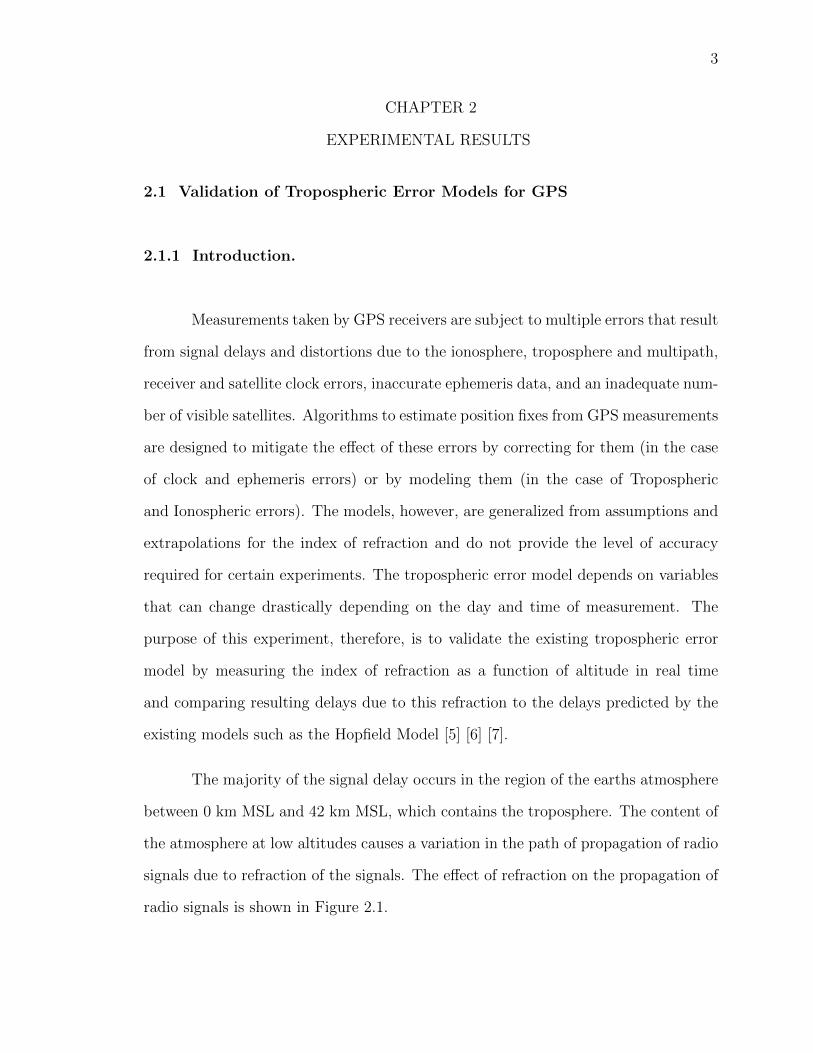
The majority of the signal delay occurs in the region of the earths atmosphere

between 0 km MSL and 42 km MSL, which contains the troposphere. The content of

the atmosphere at low altitudes causes a variation in the path of propagation of radio

signals due to refraction of the signals. The effect of refraction on the propagation of

radio signals is shown in Figure 2.1.

4

Figure 2.1. Diagram showing how electromagnetic signals are affected by refractionas they pass through the lower atmosphere. [4]

The Tropospheric Error affecting a GPS measurement consists of two primary

parts, the Wet Tropospheric (TW) delay and the Dry Tropospheric (TD) delay. The

wet tropospheric delay is the major contributing factor up to an altitude of 12 km MSL

due to the existing water vapor whereas the dry tropospheric delay contributes the

most at altitudes above 12 km MSL. The total Tropospheric Error (T ) is calculated

by adding up the two components. Tropospheric error for a radio signal traveling

along the path of a 90 degree Elevation angle, an angle measured from the horizon,

can be estimated by the following equation:

T = 10−6∫

[ND(h) + NW (h)]dh (2.1)

5

where T is the total Tropospheric error (meters), ND is the dry component of the

index of refraction, NW is the wet component of the index of refraction and h is the

height from the receiver (in meters).

The challenge is to accurately calculate the dry and wet components of the

indices of refraction in order to be able to achieve an accurate result for the tropo-

spheric error. These components can be calculated using equations derived by Rueger

[11]:

N = 77.6890P

T− 6.3938

PWT

+ 3.7546 ∗ 105 PWT 2

(2.2)

where N is the total index of refraction, P is the total pressure (in millibars), PW

is the partial pressure of water (millibars), T is the absolute temperature (K). The

partial pressure of water vapor can be calculated by using the equations derived by

Buck [1]:

esat = 6.1121 (1.0007 + 3.46 ∗ 10−6 Po) e17.502 ToTo+240.97 (2.3)

PWo = esat

[1 − (1 −RH)

esatPo

]−1

RH (2.4)

where esat is the saturation vapor pressure (millibars), RH is the relative hu-

midity, PWo is the partial pressure of water vapor (millibars).

6

2.1.2 Analysis Procedure.

The experimental setup consisted of three sensors measuring the atmospheric

pressure, temperature and humidity against the altitude of the payload, also recorded

through GPS measurements.

Figure 2.2. Representation of the experimental setup for tropospheric error measure-ment.

The analysis procedure is as follows:

1. Extract data necessary to calculate index of refraction and tropospheric error

from the file

2. Filter out blank spaces in data (i.e. NaN values) and remove any anomalous

data.

3. Once data is pre-processed, calculate the index of refraction

7

2.1.3 Results and Discussion.

The analysis conducted required a few critical decisions in order to extract

valid results. Due to sparsity of data available and issues with time synchronization,

there was a significant amount of anomalous data in the ascent and descent phases

of the flight. Therefore data collected during the steady phase of flight was analyzed.

The results still are inconsistent due to possible errors in the data used, regardless of

significant pre-filtering.

Figure 2.3. Altitude vs time index (in seconds

8

Pressure, temperature, relative humidity data was used to calculate the index

of refraction (N). The pressure and temperature data followed trends as known in

scientific literature with slight variations. However, the relative humidity (RH) data,

which is one of the most critical elements in evaluating N, was inconsistent. This

significantly affected the calculations for index of refraction. A noticeable relation

between trends of change in altitude and change in index of refraction is visible.

For the ascent and descent phases of flight, as the altitude increases the value of

N decreases and vice-versa. This is because the moisture content of air decreases

as altitude increases and therefore reduces the possibility of refraction incidences.

During the steady phase of the flight at very high altitudes, the value of N held

relatively constant. However, the values are constantly below N = 1. The index of

refraction of vacuum is 1, meaning that a signal does not get refracted. Values below

one should not be possible for the type of signal frequencies (L1 GPS frequency) and

signal power in use. A best guess attempting to reason the occurrence of this error is

anomalous relative humidity data.

A final step of analysis, integrating index of refraction over the signal path

to calculate the actual tropospheric error, is not possible due to three reasons. The

biggest reason for the inability to calculate tropospheric error is the significant lateral

movement of the balloon during the flight phase. An accurate model of error was

contingent upon multiple data points being collected at close locations, i.e. when the

lateral motion of the balloon was slow. For this HASP flight, the balloon traveled

long distances over the duration of the mission. Adding the lack of data to the

balloons motion negated any chance of calculating a meaningful tropospheric error

model. Another major reason is the lack of means to differentiate between different

GPS satellites. And the final reason is the error in evaluating index of refraction.

The team was unsuccessful in evaluating and comparing tropospheric error to

9

Figure 2.4. Index of refraction vs. time index (in seconds)

widely accepted error models. There were multiple events gone wrong that caused

a stack effect in rendering the data invalid for calculating the tropospheric error.

However, some results were successfully obtained from the data available for analysis.

After significant pre-filtering, tentative values for the index of refraction as a function

of altitude were obtained. These values followed general trends expected of the index

of refraction within an approximate range of the true values of index of refraction

and would have been much more accurate given a functioning humidity sensor. This

result validated the choice of mathematical expressions used to evaluate the index of

refraction. For these reasons, the experiment can be called a partial success.

10

2.2 Measurement of Stratospheric Methane and Water Vapor

2.2.1 Introduction.

Methane is the most common hydrocarbon trace in the atmosphere, which

along with water vapor, contributes significantly to the Earths greenhouse effect. In

the last 50 years, there has been a yearly 1% increase in stratospheric water vapor.

[2] Likewise, up to a 15% increase in atmospheric has been measured from 1978 to

1998 with significant variations at different altitudes. [10] In order to better predict

further increases and their effect on climate, a model has been developed to predict

the concentrations of methane and water vapor at different altitudes.

C H4 + 2O2 <=> 2H2O + C O2 (2.5)

The thermodynamic state of the surroundings must be known, including pres-

sure, temperature, and gas concentrations. Since the relative concentration of oxygen

remains nearly constant with altitude, the absolute concentration may be calculated

from the pressure. In Eq. 1, the reversible stoichiometric reaction shows atmospheric

methane reacts with oxygen to produce water vapor and carbon dioxide. The reaction

rate is determined by the relative concentrations of the reactants and the tempera-

ture at which the reaction takes place. Eq. 2 and Eq. 3 are the governing equations

where [A] is the concentration of some specie A, the Greek letters are the number of

moles produced or consumed per reaction, and reaction constants k are found using

the Arrhenius equation of equilibrium.

k+[C H4]α[O2]

β = k−[H2O]σ[C O2]τ (2.6)

11

k = Ae−( EaRT

)γ (2.7)

If the system is taken to be at steady state, which is a reasonable assumption, all

time derivatives are defined to be zero and the methane concentration can be found

simply using the equation:

[C H4] =

[k−[H2O]σ[C O2]

τ

k+[O2]β

] 1α

(2.8)

2.2.2 Experimental Setup.

Figure 2.5. Representation of the experimental setup for methane gas measurement.

12

The sensor package contained on SCARLET HAWK I was designed to measure

gas concentrations of methane, carbon dioxide, water vapor, as well as temperature,

pressure, and humidity. This was accomplished using a sensor package fixed at the

top of the electronics stack and open to the outside environment. Since the goal was

to measure the methane concentration and thermodynamic properties with respect to

altitude, the sensor package was designed to take data measurement during the ascent

portion of the HASP mission as well as to take some data shortly before termination.

This would allow the model to be validated for a full altitude profile.

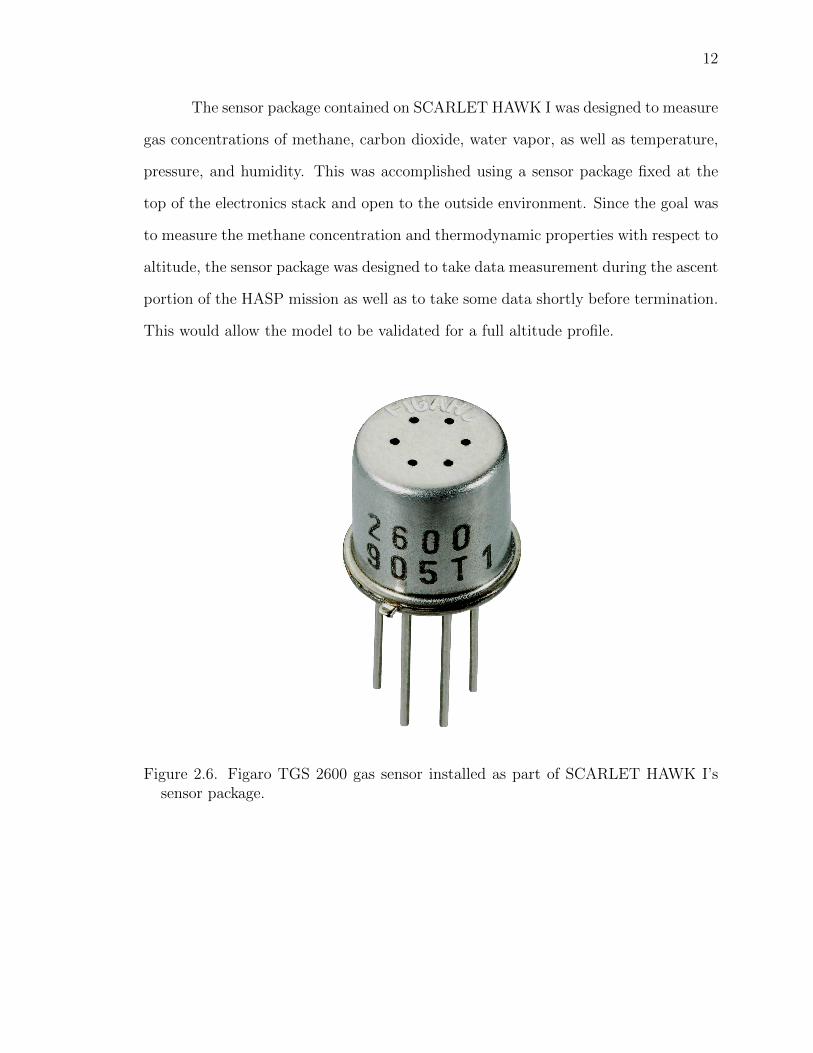
Figure 2.6. Figaro TGS 2600 gas sensor installed as part of SCARLET HAWK I’ssensor package.

13

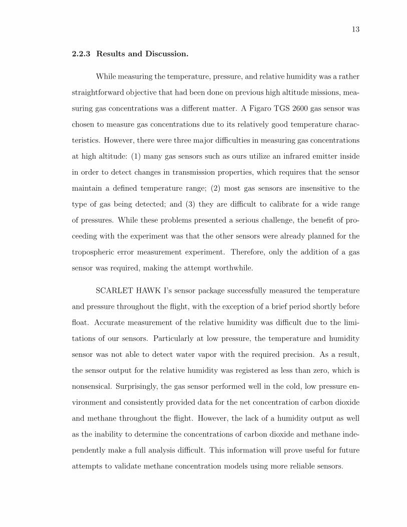
2.2.3 Results and Discussion.

While measuring the temperature, pressure, and relative humidity was a rather

straightforward objective that had been done on previous high altitude missions, mea-

suring gas concentrations was a different matter. A Figaro TGS 2600 gas sensor was

chosen to measure gas concentrations due to its relatively good temperature charac-

teristics. However, there were three major difficulties in measuring gas concentrations

at high altitude: (1) many gas sensors such as ours utilize an infrared emitter inside

in order to detect changes in transmission properties, which requires that the sensor

maintain a defined temperature range; (2) most gas sensors are insensitive to the

type of gas being detected; and (3) they are difficult to calibrate for a wide range

of pressures. While these problems presented a serious challenge, the benefit of pro-

ceeding with the experiment was that the other sensors were already planned for the

tropospheric error measurement experiment. Therefore, only the addition of a gas

sensor was required, making the attempt worthwhile.

SCARLET HAWK I’s sensor package successfully measured the temperature

and pressure throughout the flight, with the exception of a brief period shortly before

float. Accurate measurement of the relative humidity was difficult due to the limi-

tations of our sensors. Particularly at low pressure, the temperature and humidity

sensor was not able to detect water vapor with the required precision. As a result,

the sensor output for the relative humidity was registered as less than zero, which is

nonsensical. Surprisingly, the gas sensor performed well in the cold, low pressure en-

vironment and consistently provided data for the net concentration of carbon dioxide

and methane throughout the flight. However, the lack of a humidity output as well

as the inability to determine the concentrations of carbon dioxide and methane inde-

pendently make a full analysis difficult. This information will prove useful for future

attempts to validate methane concentration models using more reliable sensors.

14

Figure 2.7. Plot of temperature vs altitude.

Figure 2.8. Plot of pressure vs altitude.

15

Figure 2.9. Plot of relative humidity vs altitude. The data in this plot is obviouslyincorrect since it passes below zero. This is likely due to pressure and temperatureeffects.

Figure 2.10. Plot of carbon dioxide + methane concentration with respect to altitude.

16

2.3 Image Capture and Transmission

2.3.1 Camera System Development.

Many high altitude balloon missions have included some form of photography

or remote image capturing. This has typically required taking pictures that are

saved to an internal memory inside the payload, and retrieved after the payload

descends back to the ground. Apart from the risk of losing the payload with the

data, it is also not possible to see the images until the payload is on the ground.

However if the images can be converted into a data string and sent to a control

station on the ground, then the information can be preserved and obtained earlier in

the mission. Furthermore, for other types high altitude missions, including sounding

rocket launches and CubeSat missions, real-time image transmission is a mission-

critical requirement.

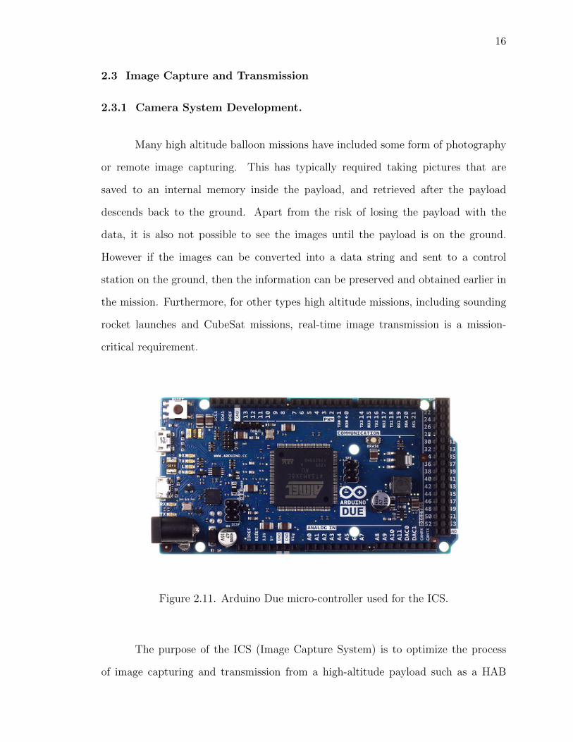
Figure 2.11. Arduino Due micro-controller used for the ICS.

The purpose of the ICS (Image Capture System) is to optimize the process

of image capturing and transmission from a high-altitude payload such as a HAB

17

payload or even a CubeSat to a ground station. This will allow the ICS to stay

within the narrow operating envelope defined by Baud rates, power consumption,

and downtime limitations. This is achieved by powering down all other non-critical

components, then using three cameras to capture images individually and transmit

the image data using the HASP serial port. For these reasons, it was decided that an

ICS be included in SCARLET HAWK I.

Figure 2.12. Representation of the experimental setup.

18

Several characteristics of the subsystem changed since the submission of the

proposal in December, 2012. The most important of these changes was the use of

a different micro-controller with a bigger SRAM and a more powerful microproces-

sor. The SRAM in the originally considered microprocessor (ATmega1280) was 8KB

compared to 96KB in the microprocessor used for the flight (AT91SAM3X8E). The

reason behind using the new microprocessor on board was that an encoding algo-

rithm, a Reed-Solomon code, was necessary to include in the original design in order

to ensure that the majority of image data would be recovered uncorrupted.

The Reed-Solomon algorithm implemented required at least 20KB of static

memory to be able to do the encoding of the 6KB pictures that were to be sent as

thumbnails to ground station. This change in microprocessor also required another

important change in the design of the payload electronics. The Arduino Mega that

was used as the master computer for the mission required serial communication at

5V, while the Arduino Due required 3V. Two level converters, to step down from

5V to 3V, had to be adapted for the serial communication between the cameras and

Arduino B, and between Arduino A and Arduino B. The final EPS for the main board

of the Image Capturing System is shown in Figure 2.12.

2.3.2 Results and Discussion.

At the beginning of this experiment, three objectives were set for this subsys-

tem:

Table 2.1. ICS Objectives

Mission Result

Capture of images in flight Successful

Image processing and storage on-board Successful

Image transmission in flight Unsuccessful

19

In total, 506 pictures were taken throughout the flight. The system was con-

figured so that the cameras take big pictures ( 40KB) during the entire flight and

small pictures ( 6KB) whenever a command were received by the microprocessor.

Both small and big pictures were found within the 506 pictures and they certainly

follow a logical sequence.

(a) Hi-Resolution ∼ 40 KB Image

(b) Low-Resolution ∼ 6 KB

Figure 2.13. Examples of a high (a) and low (b) resolution image captured in flight.

20

Of the three cameras on board, two were fully functioning. However, one of the

side cameras failed. The amperage stayed within the expected range, 0.19-0.2 amps,

during the flight. This fact led us to think all the cameras were working properly. A

post-flight analysis of the electronics in the payload, however, determined that the

TX connection of one camera unsoldered during the flight. Therefore, none of the

pictures taken by this camera were saved to the SD card on board.

Figure 2.14. Picture of the Arduino A when the payload was opened for the first timefollowing recovery.

As data transmission failed between the micro-controller in charge of trans-

mitting the data to ground (Arduino A) and the micro-controller in charge of the

image processing (Arduino B), our team was only able to see the pictures once the

payload was recovered. All the pictures taken throughout the flight were successfully

compressed and saved under the JPEG-2000 format. According to the recording rate,

there was enough storage capacity for 102 hours of flight.

The code in the Arduino B worked properly during the flight test and the

21

actual flight. All of the 5 commands sent from ground station to switch from big

to small pictures and vice versa were totally executed and processed by the micro-

controller. The evidence for this can be observed in each of the three folders (one

per each camera) containing exactly 5 small pictures that were to be used as thumb-

nails. Problems with the code run by the Arduinos as well as with the Reed-Solomon

algorithm on board were discarded after confirming that the data in the SD card

fully matched the logic behind these codes. Name sequence (files were name after a

logical increasing sequence), timestamps and number of files showed that Arduino B

successfully received the commands, managed to take, stored, encode and forward the

pictures to Arduino A, but Arduino A did not receive the transmitted thumbnails.

The fact that every time that a command was sent to switch to small pictures

the command was executed and the thumbnails encoded but the images were not

going through HASP Channel suggested that a possible cause of the failure was in

the communication between Arduino A and Arduino B. The only electrical compo-

nent between both micro-controllers was the level converter. Once the region of the

issue was identified, continuity was checked between all the TX and RX connections.

Communication between the Transmission port of the Arduino B and the Reception

port of the level converter proved to be working fine in a post-flight test. The connec-

tions between Arduino A and the level converter were also working properly after the

flight. The entire system was run again and no communications issues were detected.

It should be noted that the connection between both micro-controllers worked per-

fectly during the thermal-vacuum test. The failure in the level converter might have,

then, been due to specific flight conditions.

The temperature range during the time the commands were sent was from

29C to 45C inside the payload while it stayed steady around 29C for the exterior

temperature during the same period. During this time, the pressure also stayed close

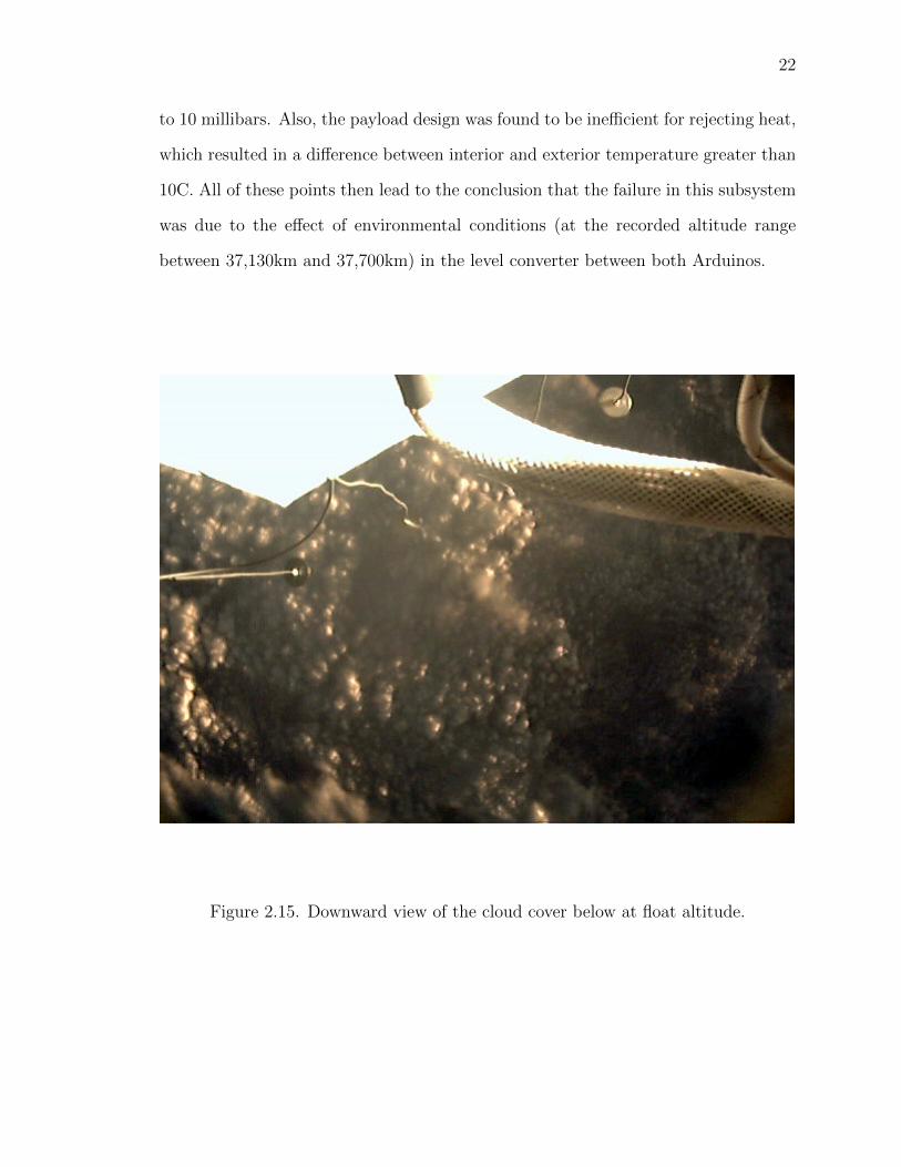
22

to 10 millibars. Also, the payload design was found to be inefficient for rejecting heat,

which resulted in a difference between interior and exterior temperature greater than

10C. All of these points then lead to the conclusion that the failure in this subsystem

was due to the effect of environmental conditions (at the recorded altitude range

between 37,130km and 37,700km) in the level converter between both Arduinos.

Figure 2.15. Downward view of the cloud cover below at float altitude.

23

(a) High resolution image of the horizon taken during float at 130,000 ft.

(b) Southwestern view at dusk, with Venus visible near the upper right corner.

Figure 2.16. Side view images taken during the flight.

24

(a) View of the sunset at 130,000 ft.

(b) View of the horizon and the ground below at sunset.

Figure 2.17. Side view images taken during the flight.

25

CHAPTER 3

PAYLOAD DESIGN EVALUATION

3.1 SCARLET HAWK I

The payload electronics was comprised of four printed circuit boards, contain-

ing the on board computer, power management system, image capture system, and

sensing circuits. At different times throughout the mission, the payload ran on one

of two different modes of operation: Sensor Mode or Camera Mode. This layout

and mode of operation helped to conserve space, weight, and electrical power. Fur-

thermore, utilizing a stacked system of printed circuit boards helped to minimize the

number of free wires in the payload and likely prevented shorted circuits as well as

other mishaps. The only major problem with this layout is that the stack had to be

pulled out of the structure in order to reach the SD cards or any of the computer

ports. The lack of practical accessibility to the hardware also made it more difficult

to replace malfunctioning electronics during the testing and integration phase.

Two Arduino microcomputers provided all on-board computing, with an Ar-

duino Mega serving as the master computer that controlled whether the payload was

in sensor or camera mode. An Arduino Due was required to control the image cap-

ture system since more SRAM was needed for the Reed-Solomon algorithm. While

this was actually a good idea in itself, problems emerged due to the fact that the

Arduinos operated using different serial voltages. This required the inclusion of a

level converter that later failed, causing problems for the GPS and image capture

systems later on.

In retrospect, we realize that carbon fiber was not a good material to use

for the entire structure. It carried a considerable portion of the overall cost of the

payload and made thermal management difficult. Painting the surface of the carbon

26

fiber was found to be nearly impossible, with the paint actually peeling off during

thermal-vacuum testing. Eventually, tape was used to cover the dark colored exterior

in order to minimize sunlight absorption. Carbon fiber also proved to be relatively

difficult to work with, since manufacturing errors were very expensive because of the

cost of the material. In terms of strength, SCARLET HAWK I’s structure was clearly

over-engineered for the actual mission requirements.

One of our most serious errors was assuming that the cold temperatures were

most likely to cause problems with electronics. During testing as well as the mission,

overheating was likely the culprit behind some of the malfunctions that occurred

during the flight. One of the main failures, for example, was the level converters

in the image capture system and this was due to overheating. One way of tackling

this issue would be attaching heat sinks to the critical components of the system and

developing a way of rejecting heat out of the payload.

3.2 Proposed Changes for SCARLET HAWK II

1. A more practical access to the memory cards and uploading ports should be

implemented in future payloads, likely using easily removable panels .

2. More effort should focus on heat management in general and rejection of heat

from critical components in particular.

3. Effort should be made to quickly produce prototype electronics, so they can

undergo rigorous testing early in the design process. Testing their performance

at different critical conditions (e.g. high temperatures) would certainly avoid

problems like the one of the GPS and the level converters.

27

Figure 3.1. Region where the ports and SD cards were located inside the red box,out of reach of the top or bottom openings.

4. In order to eliminate the need for level converters (that can fail), all on-board

computers should operate with a common serial voltage.

5. The management structure of future teams should include greater delegation

of responsibilities. Emphasis should be placed on developing leadership skills

throughout the team from top to bottom. These skills are important for engi-

neers and are not learned in the classroom.

6. Design schedules should be planned more aggressive deadlines, since the team

lost a great deal of manpower once the summer break had begun.

28

7. Future structural design should favor simpler construction and more commonly

available materials. Mechanical fasteners should be chosen over less reliable and

more permanent epoxying.

8. More focus and less broad mission objectives should be aimed at for future

endeavors. This will leave more energy and resources to successfully accomplish

all of the mission goals.

29

3.3 Looking Forward

SCARLET HAWK I served as AIAA-IIT’s first payload for a HASP mission

and collected data for several missions simultaneously. In the areas where the payload

functioned well and successfully completed its goals, SCARLET HAWK I proved the

teams ideas and designs. The aspects of the payload that did not perform satisfacto-

rily also allowed the team to understand our mistakes and develop alternative designs

for future missions. Above all, AIAA-IIT was able to pass integration and fly on the

2013 HASP mission without a critical system failure. We are now familiar with the

process of designing a payload for a HASP mission and understand the opportunities

that will be available next year.

Now that the mission has been completed, the hard work of planning for a

HASP 2014 mission must begin. This work has been detailed in a proposal which

will be delivered to HASP coordinators on December 20, 2013. With the beginning of

a new year, AIAA-IIT’s Space Technology Program will continue to actively recruit

and train new members. These new members can be expected to play a large part in

the design of SCARLET HAWK II and will apply the lessons we have learned this

year.

30

APPENDIX A

2013 AIAA-IIT TEAM DEMOGRAPHICS

31

Table A.1. AIAA-IIT Demographics Data

Last Name First Name Gender Ethnicity Race Status Disability

Arnaout Abdulrhaman M Non-Hispanic Caucasian Grad N

Borate Shalmikraj M Non-Hispanic Indian Grad N

Finol David M Hispanic Latino Undergrad N

Garcia Jesus M Hispanic Latino Undergrad N

German Joshua M Non-Hispanic African Undergrad N

Grimaud Lou M Non-Hispanic Caucasian Grad N

Haider Qasim M Non-Hispanic Asian Undergrad N

Javier Miguel M Non-Hispanic Asian Undergrad N

Katre Aniruddha M Non-Hispanic Indian Grad N

Kozak Peter M Non-Hispanic Caucasian Grad N

Lin Senbao M Non-Hispanic Asian Grad N

Manotas Rodolfo M Hispanic Latino Undergrad N

Page Corey M Non-Hispanic Caucasian Undergrad N

Rutenbar Colin M Non-Hispanic Caucasian Undergrad N

Singh Manpreet M Non-Hispanic Indian Grad N

Venet Teva M Non-Hispanic Caucasian Undergrad N

Vitto Raisa F Non-Hispanic Indian Grad N

32

APPENDIX B

HASP 2013 STUDENT IMPACT

33

B.1 Impact Statements

B.1.1 Abdulrhaman Arnaout - EECE Graduate Student.

HASP project made me realize how vast studying the behavior of electronic

pieces on high elevations is. So I could now imagine how different it will be in the

far space! My experience with Scarlet Hawk team was amazing; I have seen so many

students working very hard on this project despite the fact that they have so much

load coming from their other classes, and this project doesn’t count toward their

degree; and yet, they were always excited, enthusiastic, and happy! The moment

when you try what you built, and it does work, you just feel fantastic.

B.1.2 David Finol - MMAE Undergraduate Student.

The HASP program has certainly helped me develop my professional skills and

get a taste of what it will be like after school. The fact that there is no second chance

in a flight and that there are efforts of an entire team in risk truly pushes me to make

the most out of the flight. The program allows us to get acquainted with space-like

conditions and definitely gives the hands-on experienced to tackle all the challenges

brought by those conditions. The very professional and punctilious way Dr. Guzik

and his team manages the program also made it a fruitful experience for me.

B.1.3 Qasim Haider - EECE Undergraduate Student.

Working in HASP 2013 has had such an immense affect on my academic life,

I have learned so much while working on the project. It has really broadened the

horizons of my mind and taught me that ’sky is the limit!’

34

B.1.4 Miguel Javier - MMAE Undergraduate Student.

The HASP program that I have been a part of has allowed me to put to use

my CAD knowledge and design class to be able to design and build the payload for

the project. Additionally being able to go through the design build process all the

way through the completion of the project has allowed me to see the project through

until the end.

B.1.5 Aniruddha Katre - MMAE Graduate Student.

HASP was a very exciting experience because it gave me the chance to help

take a product through the complete design, manufacturing, assembly and testing

phase. Also, the the experience of working in a team environment with the freedom

to innovate and apply the knowledge gained from academics in a practical setting

relevant to my academic background was invaluable.

B.1.6 Senbao Lin - MMAE Graduate Student.

Working on AIAA-IIT’s HASP mission has:

1. Enhanced my communication skills

2. Improved my time management skills

3. Gave me new perspective to look at technology

B.1.7 Rodolfo Manotas - MMAE Undergraduate Student.

Participating in HASP allowed me to get a better understanding of how en-

gineering knowledge can be applied to a project involving designing an experiment.

Working in a team with graduate students and other students both below and above

35

my level, with multiple talents and in different disciplines, gave me a great deal of

experience and gives me an idea of what my future challenges in engineering could

be like. Finally, being able to interact with teams from other universities helped us

to see things from other points of view and also to exchange a few ideas among each

other.

B.1.8 Colin Rutenbar - CAEE Undergraduate Student.

HASP definitely gave me a an outlet for skills outside of my major and to help

a team accomplish a goal. It has prepared me for working in an IPRO as well as

working with multiple levels of education (from freshmen to PhD candidates) and to

work in a multicultural group.

36

BIBLIOGRAPHY

[1] Buck, A. L. (1981). New equations for computing vapor pressure and enhance-ment factor. Journal of Applied Meteorology, 20(12), 1527-1532.

[2] Kley, D., & Phillips, C. (Eds.). (2000). SPARC assessment of upper troposphericand stratospheric water vapour. SPARC office.

[3] Kuo, K. K. (1986). Modeling Oxidation Chain Reaction. Principles of combus-tion.

[4] Hohenkerk, C. Y., & Sinclair, A. T. (1985). The Computation of an AngularAtmospheric Refraction at Large Zenith Angles. HM Stationery Office.

[5] Hopfield, H. S. (1969). Two-quartic tropospheric refractivity profile for correct-ing satellite data. Journal of Geophysical research, 74(18), 4487-4499.

[6] Hopfield, H. S. (1971). Tropospheric effect on electromagnetically measuredrange: Prediction from surface weather data. Radio Science, 6(3), 357-367.

[7] Hopfield, H. S. (1972). Tropospheric refraction effects on satellite range mea-surements.

[8] Mangum, J. (2009). Atmospheric refractive signal bending and propagationdelay. Report, National Radio Astronomy Observatory (NRAO).

[9] Milbert, D. (2012). Sources of Errors in GPS. GPS Explained: Error Sources.

[10] Riese, M., Grooss, J. U., Feck, T., & Rohs, S. (2006). Long-term changes ofhydrogen-containing species in the stratosphere. Journal of atmospheric andsolar-terrestrial physics, 68(17), 1973-1979.

[11] Rueger, J. M. (2002). Refractive index formulae for electronic distance measure-ment with radio and millimetre waves. Unisurv Report S-68, School of Survey-ing and Spatial Information Systems, University of New South Wales, UNSWSYDNEY NSW, 2052, 1-52.

[12] Stewart, M. F. (2009). Time and Position Data String Serial Latency Measure-ments. HASP Technical Report 2009-01