2012 Course:

The Statistician Brain: The Bayesian Revolution in Cognitive Sciences

Stanislas Dehaene

Chair of Experimental Cognitive Psychology

Lecture n°6

The neuronal implementation of Bayesian mechanisms

Lecture material translated from the French version by CG Traduction & Interprétation

What are the characteristics of a « Bayesian » decision?

Bayesian Inference: • All sensory cues provide

probabilistic evidence which constrains the interpretation of the physical world.

• These fragments of evidence combine with each other according to Bayes rule

• … and with the priors we may have on the state of the world

Gain Function:

• Motor tasks apply a gain or loss function

• We try to choose the action which maximizes expected gain.

Do our actions reflect the Bayes-optimal integration?

Körding & Wolpert (2004): Subjects attempt to reach a target while their finger is moved over an unknown distance Insertion of two sources of movement uncertainty: - The starting point is randomly moved (mean = 1 cm, standard deviation = 0.5 cm) - Midway through the experiment, subjects are given information on the position of their finger which can be:

- precise - uncertain - absent Kording, K. P., & Wolpert, D. M. (2004). Bayesian integration

in sensorimotor learning. Nature, 427(6971), 244-247.

Do our actions reflect the Bayes-optimal integration? What does the Bayesian model predict? -The a priori distribution of shifts is a Gaussian curve centered on +1 cm.

- Example of feedback received in the case of an initial shift of 2 cm. Bayes’ rule predicts a combination of two distributions according to the product rule. According to the level of uncertainty of the central point, subjects should compensate only in part for the perceived position.

Kording, K. P., & Wolpert, D. M. (2004). Bayesian integration in sensorimotor learning. Nature, 427(6971), 244-247.

a priori

feedback

a posteriori

Do our actions reflect the Bayes-optimal integration?

Predictions of the Bayesian model: - when perception is precise, subjects compensate adequately for the initial side movement, and the final deviation from the target is minimal (purple curve) - as sensory uncertainty grows, subjects take less and less into account the information on the central point, and return to the prior (1 cm of deviation on average)

Final target deviation

Two other possible models - Full trade-off: subjects use all the available information on the central point. The average is accurate but mean error increases. - Learning on the basis of the final position: since it is given only in the “precise” condition, subjects should behave in the same way whatever the level of uncertainty.

Full trade-off model Learning model

Do our actions reflect the Bayes-optimal integration?

Predictions of the Bayesian model: - when perception is precise, subjects compensate adequately for the initial side movement, and the final deviation from the target is minimal (purple curve) - as sensory uncertainty grows, subjects take less and less into account the information on the central point, and return to the prior (1 cm of deviation on average)

Final target deviation

The results of the experiment comply with the Bayesian model.

Do our actions reflect the Bayes-optimal integration?

Experiment 2: non-Gaussian a priori distribution The optimal response is more difficult to apprehend. It is non-linearly dependent on the perceived position. This is precisely what we observed! The brain may be able to carry out Bayesian computations via average distributions (?)

un sujet le groupe

q(n)

w(n) . . . . . . .

Criteria small large

All decisions imply Bayesian inference: Evidence accumulated during a single trial

Central Integration (C) Motor stage (M)

Perceptual stage (P)

RT Distribution

Stimulus Response P

C

M

• Many Bayesian problems can therefore be reduced to an internal random walk: - Each sample positively or negatively modifies the accumulated evidence in favor of the different response options

- Optimal decisions can be made when the threshold of total accumulated evidence is reached.

• If there are several successive and independent samples, X1, X2, X3… then Bayes’ theorem is an easy way to accumulate this data:

• P(R| X1, X2, X3 …) is proportional to product P(R) P(X1 | R) P(X2| R) P(X3| R) … • With a logarithm, the evidence provided by each sample is summed up.

• Even the simplest decision (such as, are dots moving to the left or to the right?) may require the combination of several samples according to a Bayesian rule.

• In fact, the occurrence of fluctuations (in the stimulus or in the nervous system) leads to ambiguous decisions, and requires computing the most plausible response

The monkey must decide in which direction the dots move. Motion coherence modulate the firing rate of neural responses during the decision-making process.

Fixed Threshold Decision

Variable speed Accumulation

Prefrontal and parietal neurons compile statistics relevant to decision-making

Kim & Shadlen, Nature Neuroscience 1999

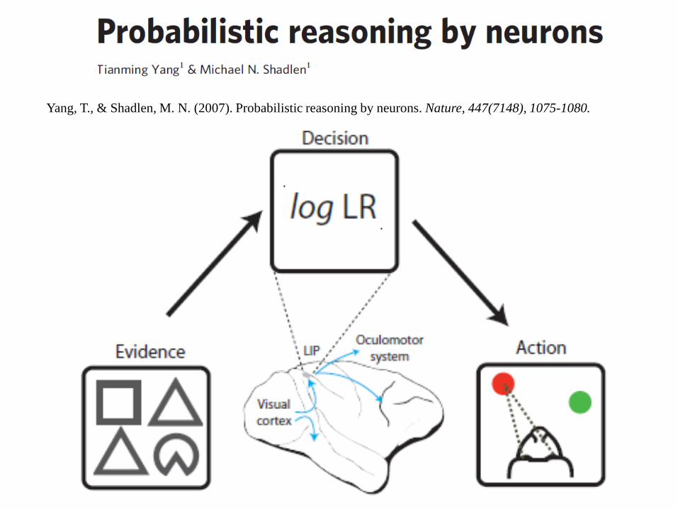
Yang, T., & Shadlen, M. N. (2007). Probabilistic reasoning by neurons. Nature, 447(7148), 1075-1080.

Do neurons in the LIP area of the cortex compute a genuine Bayesian inference? Can they combine several sources of probabilistic information ?

Task inspired by the human task of “weather reporting”. In each round, the monkey is shown 4 shapes sequentially,

selected among 10 other possible shapes. Then the monkey makes a saccadic eye movement towards the

red or green dot. Reinforcement is not certain, but provided via a probabilistic rule

which depends on the sum of the cues provided by each shape.

The evidence (weight of evidence [WOE] or log posterior odds) is equal to the sum of the weights:

The number of shape combinations (104

permutations, 715 combinations) encourages the inference of a general rule on behavior.

Yang, T., & Shadlen, M. N. (2007). Probabilistic reasoning by neurons. Nature, 447(7148), 1075-1080.

Yang, T., & Shadlen, M. N. (2007). Probabilistic reasoning by neurons. Nature, 447(7148), 1075-1080.

After several thousand training exercises, monkeys respond in a more probabilistic and regular manner.

Their response rate is a sigmoidal function of the objective evidence [WOE].

It can be modelled through logistic regression.

Subjective weights assigned to each shape are closely correlated with the objective weights.

When neurons implement probabilistic reasoning

Yang, T., & Shadlen, M. N. (2007). Probabilistic reasoning by neurons. Nature, 447(7148), 1075-1080.

Recording of neurons in the LIP area, where the receptor field includes one of the targets of the saccade.

Assumption: the rate of neural firing reflects the evidence accumulated at all times:

The quantity is approximately equal to the sum of

n cues received (exactly for n = 4). Indeed: 1. Neural firing reflects whether the selected

target is within the visual field or not.

When neurons implement probabilistic reasoning

Yang, T., & Shadlen, M. N. (2007). Probabilistic reasoning by neurons. Nature, 447(7148), 1075-1080.

2. Neural firing tracks the value of the evidence at all times (divided in quintiles).

When neurons implement probabilistic reasoning

3. The firing rate of this neuron varies linearly as a function of the evidence.

Yang, T., & Shadlen, M. N. (2007). Probabilistic reasoning by neurons. Nature, 447(7148), 1075-1080.

When neurons implement probabilistic reasoning

Movies of neural activity during several trials

Yang, T., & Shadlen, M. N. (2007). Probabilistic reasoning by neurons. Nature, 447(7148), 1075-1080.

When neurons implement probabilistic reasoning

Movies of neural activity during several trials

Yang, T., & Shadlen, M. N. (2007). Probabilistic reasoning by neurons. Nature, 447(7148), 1075-1080.

When neurons implement probabilistic reasoning

Movies of neural activity during several trials

Yang, T., & Shadlen, M. N. (2007). Probabilistic reasoning by neurons. Nature, 447(7148), 1075-1080.

When neurons implement probabilistic reasoning

More in-depth analyses demonstrate that -Each animal has learnt the subjective weight of each shape, deviating slightly from reality. - the identification of these subjective weights facilitates predictions on the final choice - and the predictions are further improved by fluctuations in the neural firing rate: “A variation of 1 spike per second from a single neuron was equivalent to 0.1 ban of evidence” Conclusions: -Simple decisions are indeed made on the basis of accumulated evidence -The firing rate of LIP neurons approximates the “random walk” process postulated in many decision-making models (See Ratcliff) - the neural firing rates seem to be proportional to the logarithm of the log likelihood ratio. - Results do not exclude simpler or complementary interpretations

- coding of expected reinforcement - “naïve” addition of the probability that a given shape leads to reinforcement.

How do neurons code and handle probability distributions?

In primates, neuronal circuits (certainly those of other species) must enable: 1. The representation of several probability

distributions 2. The calculation, on the basis of these

distributions, of: - the product of two distributions p(H|t,v) α p(H|t)P(H|v) - Or equivalent, the addition of their

logarithm, - Between sensory modalities or over

time 3. The incorporation of a prior

p(H|D) α p(D|H) p(H) 4.The identification of the maximum a

posteriori (MAP) of the distribution

Probability coding by a population of neurons

Beck, J. M., Ma, W. J., Kiani, R., Hanks, T., Churchland, A. K., Roitman, J., et al. (2008). Probabilistic population codes for Bayesian decision making. Neuron, 60(6), 1142-1152.

An external stimulus (such as the speed of a group of dots) is represented by a firing rate vector:

r={r1,r2,…,rn}

Average Activity Activity during a given

trial

-45 0 45 0

20

40

60

80

100

Stimulus -45 0 45

0

20

40

60

80

100

Preferred stimulus

Poisson’s law applied to the cortex

Trial 1

Trial 2

Trial 3

Trial 4

For an isolated neuron, the fluctuations in neural firing rate follow a “Poisson-like” law (belonging to the “exponential family” of distributions) p(r|s) (where r is the number of action potentials observed over a given time interval) follows an asymmetrical bell-shaped curve where variance is proportional to the mean. The proportionality factor, known as Fano’s factor, varies between 0.3 et 1.8.s

Courtesy of Alex Pouget

Probabilistic neuronal population codes

-45 0 45 0

20

40

60

80

100

Stimulus

Average activity

-45 0 45 0

20

40

60

80

100

Preferred stimulus

Activity during a given trial

( )|p s ∝r ( )|p sr-45 0 45 0

20

40

60

80

100

r

-45 0 45 0

0.02

0.04

Inferred stimulus

probability

Bayesian Decoder

p(s|r)

Preferred stimulus

Assumption: via Bayes’ rule, the firing rates of a neuronal population constitute a representation of probability distribution over the space of stimuli?

Ma, W. J., Beck, J. M., Latham, P. E., & Pouget, A. (2006). Bayesian inference with probabilistic population codes. Nat Neurosci, 9(11), 1432-1438.

An external stimulus (such as the speed of a group of dots) is represented by a firing rate vector:

r={r1,r2,…,rn}

Probabilistic neuronal population codes

-45 0 45 0

20

40

60

80

100

Preferred stimulus

Activ

ity

-45 0 45 0

0.02

0.04

Inferred stimulus

Bayesian Decoder

Reduced gain: Low certainty

P(s|

r)

-45 0 45 0

20

40

60

80

100

Preferred stimulus

Activ

ity

-45 0 45 0

0.02

0.04

Inferred stimulus

P(s|

r)

Bayesian Decoder

High gain: High certainty

g

s

The gain (or intensity) of neural firing rates automatically encodes the width of the Gaussian curve that plots the plausibility of stimuli: g is proportional to 1/σ²

Ma, W. J., Beck, J. M., Latham, P. E., & Pouget, A. (2006). Bayesian inference with probabilistic population codes. Nat Neurosci, 9(11), 1432-1438.

Automatic combination of two cues

-45 0 45 0 20 40 60 80

100

Preferred stimulus

Activ

ity

g=g1+g2

+ -45 0 45 0

20 40 60 80

100

Preferred stimulus

Activ

ity g1 Vision

-45 0 45 0 20 40 60 80

100

Activ

ity

g2 Touch

Preferred stimulus 2

1 gσ

∝ 1 2g g= +2 21 2

1 1σ σ

∝ +

If neural firing rate variability is part of the exponential family, then the arithmetic sum of the firing rates of two neuronal populations can automatically compute the product of the distributions they represent.

Ma, W. J., Beck, J. M., Latham, P. E., & Pouget, A. (2006). Bayesian inference with probabilistic population codes. Nat Neurosci, 9(11), 1432-1438.

Evidence Accumulation and Selection of the Optimal Response Beck, J. M., Ma, W. J., Kiani, R., Hanks, T., Churchland, A. K., Roitman, J., et al. (2008). Probabilistic population codes for Bayesian decision making. Neuron, 60(6), 1142-1152.

MT provides an instantaneous estimation of motion, with a firing rate that is contrast-dependent.

We would like the LIP area to accumulate evidence and code the probability distribution of each motion.

We would like the superior colliculus to only represent the maximum of this distribution.

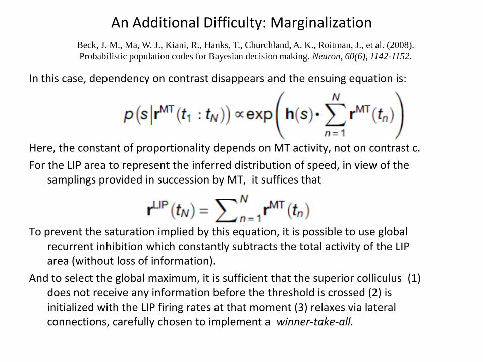
An Additional Difficulty: Marginalization

Neural firing of MT neurons depends on the direction of motion (s) as well as on other « nuisance » parameters such as contrast (c). We would like to compute the a posteriori probability of speed, in view of the contrast and firing rates observed. Or better yet, the distribution of s where the nuisance variable c has been marginalized This would be ideal, if other areas of the brain are to use the signals of MT as a speed indicator, without having to factor in the level of contrast c Beck et al. observe that all such issues are solved when function p(r) belongs to the exponential family Poisson’s law, characteristic of the neural discharges experimentally observed, belongs to this family.

Beck, J. M., Ma, W. J., Kiani, R., Hanks, T., Churchland, A. K., Roitman, J., et al. (2008). Probabilistic population codes for Bayesian decision making. Neuron, 60(6), 1142-1152.

An Additional Difficulty: Marginalization

In this case, dependency on contrast disappears and the ensuing equation is: Here, the constant of proportionality depends on MT activity, not on contrast c. For the LIP area to represent the inferred distribution of speed, in view of the

samplings provided in succession by MT, it suffices that To prevent the saturation implied by this equation, it is possible to use global

recurrent inhibition which constantly subtracts the total activity of the LIP area (without loss of information).

And to select the global maximum, it is sufficient that the superior colliculus (1) does not receive any information before the threshold is crossed (2) is initialized with the LIP firing rates at that moment (3) relaxes via lateral connections, carefully chosen to implement a winner-take-all.

Beck, J. M., Ma, W. J., Kiani, R., Hanks, T., Churchland, A. K., Roitman, J., et al. (2008). Probabilistic population codes for Bayesian decision making. Neuron, 60(6), 1142-1152.

Simulation of the Proposed Network Beck, J. M., Ma, W. J., Kiani, R., Hanks, T., Churchland, A. K., Roitman, J., et al. (2008). Probabilistic population codes for Bayesian decision making. Neuron, 60(6), 1142-1152.

Simulated firing rates Actual recordings

Conclusion: Points to Remember Beck, J. M., Ma, W. J., Kiani, R., Hanks, T., Churchland, A. K., Roitman, J., et al. (2008). Probabilistic population codes for Bayesian decision making. Neuron, 60(6), 1142-1152.

The type of neural coding and network proposed by Alex Pouget et al. calculates exactly and at all times, the a posteriori probability distribution of the speed of the stimulus: -Even if the contrast varies constantly - without needing to know or estimate this contrast - without knowing how much time has elapsed since the start of the trial

Moreno-Bote et al (PNAS, 2011) show that similar principles apply to sampling when perception is multi-stable.

Xiao-Jing Wang et al. propose more realistic networks on the neurobiological level, which approximate a similar function.

This is only true if the variability of neural firing rates r in a neuron population follows a stimulus-specific distribution belonging to the “exponential family”.

Appendix: How to Model Bayesian sampling? Moreno-Bote, R., Knill, D. C., & Pouget, A. (2011). Bayesian sampling in visual perception. Proc Natl Acad Sci U S A, 108(30), 12491-12496.

For the model to sample the a posteriori distribution according to Bayes’ rule, it is necessary and sufficient that input variability is associated to stimulus s according to Bayes’ law:

or h(s) is a function of stimulus s which is only dependent on the tuning curves of neurons and on the covariance matrix of their firing rates. This family of distributions is an excellent approximation of actual neural firing (See Ma et al., Nat Neurosci 2006).

Appendix: How to Model Bayesian sampling? Moreno-Bote, R., Knill, D. C., & Pouget, A. (2011). Bayesian sampling in visual perception. Proc Natl Acad Sci

U S A, 108(30), 12491-12496.

The exponential family of distributions has two advantages: - it enables Bayesian sampling - as well as the Bayes-optimal combination of two cues

Alex Pouget’s assumption (Ma, Beck, Latham et Pouget, Nature Neuroscience 2006): The variability of neural firing rates automatically codes for probability distributions Furthermore, this variability is in the exact format required to simplify calculations - The addition of two neuron populations corresponds to the calculation of the

product of their probability distributions - The competition between the populations (winner take all) helps to choose,

approximately, the maximum probability stimulus (Denève et al., Nature Neuroscience, 1999).