2012 COURSE IN NEUROINFORMATICSMARINE BIOLOGICAL LABORATORY

WOODS HOLE, MA

GENERALIZED LINEAR MODELS

Uri EdenSridevi V. SarmaEmery N. Brown

BU Department of Mathematics and Statistics

MIT Dept. of Brain & Cognitive Sciences

MIT Division of Health, Sciences and Technology

Massachusetts General Hospital

August 15, 2012

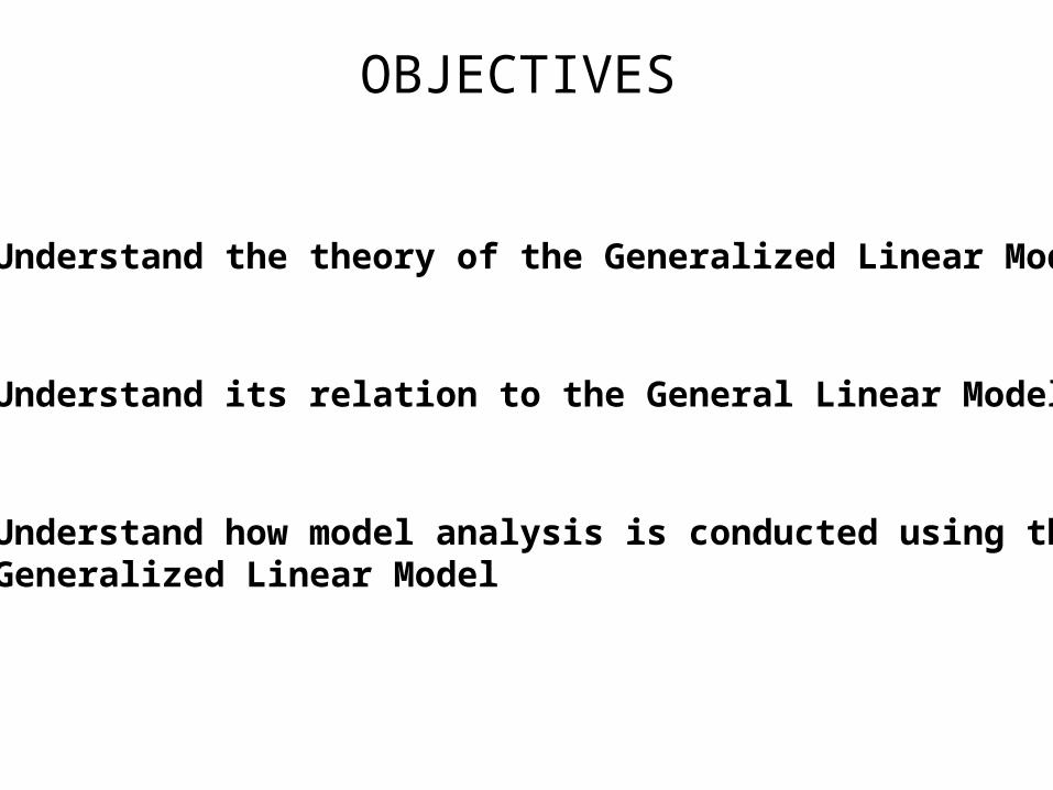
OBJECTIVES

• Understand the theory of the Generalized Linear Model

• Understand its relation to the General Linear Model

• Understand how model analysis is conducted using the Generalized Linear Model

OUTLINE

• Motivation: The Stimulus-Response Structure of Neuroscience Experiments

• Theory of the Generalized Linear Model (GLM)

• GLM Analysis of the Retinal Neuron Spike Train

• GLM Analysis of Sub-thalamic Nucleus Spike Trains in Parkinson Patients and Healthy Primate

• Summary

Spatial Receptive Fields of Hippocampal Pyramidal Neurons

Spike Histogram

0 7035

70

35

Circular Environment

0 7035

70

35

x1 (cm)x1 (cm)

x 2 (

cm)

x 2 (

cm)

Learning in Hippocampal Neurons

• Single cell recording in monkey hippocampus• Trial and error learning of association between picture

and response

Wirth et al. Science 2003Smith et al. Neural Computation 2003Smith et al. Journal of Neuroscience, 2004

Most neuroscience experiments are stimulus-response

Need a general framework that allows us to relate the stimuli in neuroscience experiments to their responses…

Experiment Stimulus/Covariate

Response

Free-behaving Rat

Position Spikes

Monkey Learning

Association Incorrect/Correct Responses, or Spikes

Goldfish Retina Constant, Spiking History

Spikes

fMRI Visual/Motor BOLD

Actually-we want to do regression for all types of data so

that we get the formal inference structure of ML (optimality, GOF, T tests on coeffs)!

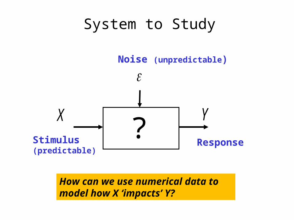
System to Study

X Y?

Stimulus(predictable)

Response

Noise (unpredictable)

How can we use numerical data to model how X ‘impacts’ Y?

From Data to Model

• Data: ),(,...),,(),,( 2211 nn YXYXYX

iscalarY

iRX

i

pi

pnn

Xn

X

X

Y

Y

Y

Y

12

11

2

1

Constant parameter vector typically estimated from data

• Notation:

s'iX

s'iY are random variables

are typically non-random variables (covariates)

From Data to Model cont…

Model is joint probability density function f:

),;( Xyf

From Linear Models to GLMs

• Linear regression models of the form:

are useful for relating Gaussian continuous valued observations to a set of covariates.

Count data:

eg. number of arrivals in time T (poisson)

Binary data:

eg. incorrect/correct response of trial (bernoulli)

~ (0, )N ),(~ XNY XY

• Generalized linear models extend a simple class of models to other data types. In particular,

• Many types of data cannot be described by a Gaussian additive noise model.

The Linear Model: A Different Perspective

1

( ) ( | ) exp{ ( ) ( ) ( ) ( )}K

k kk

L f y T y C H y D

1. Y is Gaussian which belongs to the exponential family of distributions:

2. The likelihood function for the exponential family is:

)()()()(exp)|( DyHCyTyf

Canonical Link function

Data and Parametersare multiplicatively separable!

The Linear Model: A Different Perspective cont…

12

2

1

2 2

1

1( ) exp{ ( ) }

2 2

1 exp{( { log(2 )}

2

K

k kk

K

k k k kk

L y

y y

Gaussian Data

The canonical link function is then

1

( ) ( | ) exp{ ( ) ( ) ( ) ( )}K

k kk

L f y T y C H y D

jk

p

jjkkk xXYEC ,

1

modellinear][)()(

3. The likelihood for the Gaussian and its canonical link for the linear model:

The Generalized Linear Model

1

( ) ( | ) exp{ ( ) ( ) ( ) ( )}K

k kk

L f y T y C H y D

2. The canonical link function is a linear function of the parameters

01

( )J

j jj

C x

1. Y belongs to the exponential family of distributions

All the probability models we have studied, Bernoulli, binomial, Poisson, Gaussian, gamma, exponential, inverse Gaussian, beta belong to the exponential family!

The Exponential Family

1

1

exp{ }( )

!

exp{ log( ) log( !) }

kyKk k

k k

K

k k k kk

Ly

y y

Poisson Data

The canonical link function is

1

( ) log( )J

k j kjj

C x

1

( ) ( | ) exp{ ( ) ( ) ( ) ( )}K

k kk

L f y T y C H y D

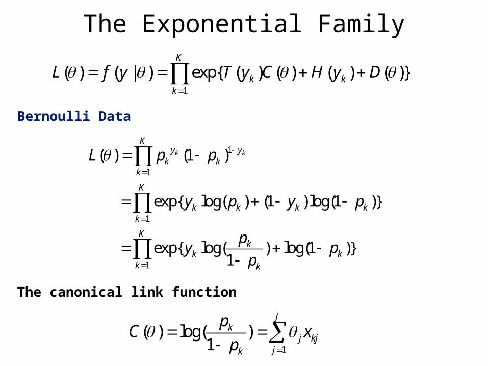
The Exponential Family

1

( ) ( | ) exp{ ( ) ( ) ( ) ( )}K

k kk

L f y T y C H y D

1

1

1

1

( ) (1 )

exp{ log( ) (1 ) log(1 )}

exp{ log( ) log(1 )}1

k k

Ky y

k kk

K

k k k kk

Kk

k kk k

L p p

y p y p

py p

p

Bernoulli Data

The canonical link function

1

( ) log( )1

Jk

j kjjk

pC x

p

1

log( )1

Jk

j kjjk

px

p

1

log( )J

k j kjj

x

1

J

k j kjj

x

Link EquationModel

Gaussian

Poisson

Bernoulli

Summary of Generalized Linear Models

Model Goodness-of-Fit and Analysis

- log (y ) - log ( )2 f | = 2

B. Akaike’s Information Criterion:

ˆ- log (y ) +ML2 f | 2p

For maximum likelihood estimates it measures the trade-offbetween maximizing the likelihood ( minimizing )ˆ- log (y )ML2 f |

and the numbers of parameters p in the model.

A. Deviance (Analog of the Residual Sum of Squares):

C. Standard Errors of the Coefficients and t-testst-statistic = Coefficient Estimate/SE

- log (y )2 f |

where in the Gaussian case

Properties of the GLM

• Convex likelihood surface• Estimators asymptotically have minimum MSE• All model estimation is efficient: iterative reweighted least

squares

Stochastic Models

Linear Regression

(output | input,history)p

Generalized Linear Models (GLM)

Neural Spiking Models

GLM Neural Models

• By selecting an appropriate set of basis functions we can capture arbitrary functional relations.

• Analysis of relative contributions of components to spiking

01

1

, ,1 1

log( ) (Extrinsic Covariates)

(Spiking History)

(Ensemble Activity)

I

k i ii

J

j jj

K C

k c k ck c

f

g

h

Truccolo W, Eden UT, Fellows MR, Donoghue JP, Brown EN. (2004) J. Neurophys 93:1074-1089

Summary of GLM Theory

• Generalization of the Gaussian Linear Model (McCulloch and Nelder)

• Can be used for any probability models in the exponential family.

• Is a maximum likelihood analysis and all its optimality properties.

• An efficient computational framework using iteratively reweighted least squares.

• GLM is available as a toolbox in all major statistics packages and Matlab.

Case 1: An Analysis of the Spiking Activity of Retinal Neurons in Culture

Retinal neurons are grown in culture under constant light and environmental conditions. The spontaneous spiking activity of these neurons is recorded. The objective is to develop a statistical model which accurately describes the stochastic structure of this activity.

(Iygengar and Liu, 1997)

Retinal Ganglion Cell Example cont…

Exponential Distribution:

Gamma Distribution:

Inverse Gaussian Distribution:

ISI Model Candidates

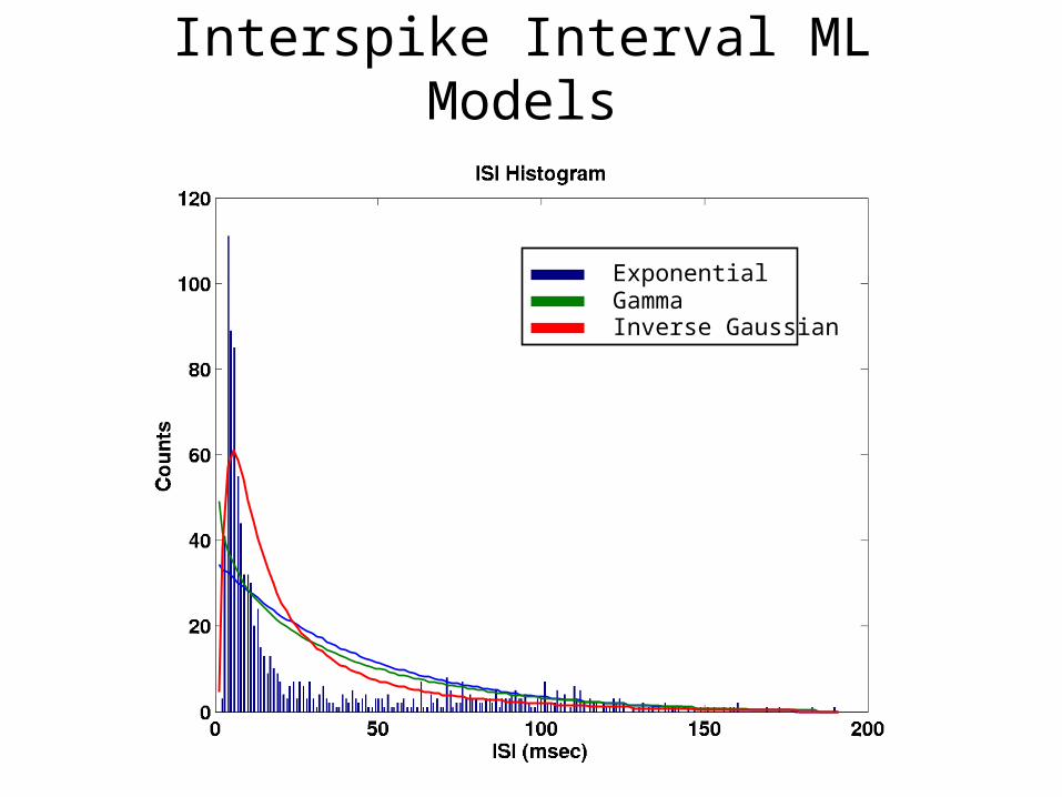
Interspike Interval ML Models

ExponentialGammaInverse Gaussian

refractoriness

short-term history

long-term history/local effects

Discrete Time Spike Train Data

dN1 dN2 dN3 dN4 dN5 dN6 dN7

0 0 1 0 0 0 1

dNk is the spike indicator function in interval k

is the intensity of spiking at time k, which in the limit is given by

k

0

Pr(Spike in ( , ) | )( | ) lim t

tt

t t t Ht H

t

Point Process is Exponential

1

(Spike Train | ) exp( log( ( | )) ( | ) )T

t u uu

L t H N u H t

Data Component

Link Function

01

exporder

k i k ii

n

Question: Can we construct a history-dependent firing rate model to describe the retinal neuron spiking activity?

How do we pick a model order?

The ISI distribution models we construct were

(ISI | ) (ISI|last spike time)tp H p

Poisson Model:

We use GLM to build history-dependent model as

0 10 20 30 40 50-0.04

-0.02

0

0.02

0.04

0.06

0.08

0.1

Model Order

Pa

rtia

l Co

rre

lati

on

Co

eff

icie

nt

Partial Correlogram-Visualization

Order=14?

Generalized Linear Model Analysis

Exploratory Analysis:

We plotted the data as a time-series.

We computed the partial autocorrelation coefficients of order up to 50.

Confirmatory Analysis:

We fit GLM models of orders varying from 1 to 120 (msec).

We computed the deviance, AIC, KS plots and the significance of the coefficients.

AIC Model Order Analysis

GLM Order

AIC

Order=14?

GLM Coefficients

Lag (msec)

Coe

ffic

ient

Val

ue

Coefficient values

Stat. significant coeffs.

Order=14?

Absolute Goodness-of-Fit

1

( | )i

i

t

i utz u H du

Time Rescale

nttt ..., 21 nzzz ..., 21

Time-Rescaling Theorem: zi’s are i.i.d. exponential rate 1

Kolmogorov-Smirnov Analysis

KS Distance is the maximum distance between an empirical and a theoretical probability model.

tan max | ( ) ( ) |dis ce nKS F u F u

Kolmogorov-Smirnov (KS) Plot:

EC

DF

(zi)

CDF(exp(1))

Graphical measure of goodness-of-fit, based on the time rescaling theorem, for comparing an empirical and model cumulative distribution function. If the model is correct, then the rescaled ISI,s are independent, identically distributed exponential 1 (uniform) random variables whose ordered quantiles should produce a 45° line.

KS distance

Empirical Quantiles

Mo

de

l Qu

an

tile

s

Kolmogorov-Smirnov Plots

Empirical Quantiles

Mo

de

l Qu

an

tile

s

KS Plots for Different Order GLMs

ISI Lag Order

Co

rrel

atio

n

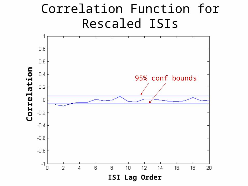
Correlation Function for Rescaled ISIs

95% conf bounds

AIC and KS Statistics

Poisson-GLM

1 14 50

6589 5931 5892

0.2525 0.0657 0.0462

Order

AIC

KS

Exp Gamma Inv. Gauss.

0.2330 0.2171 0.1063KS Statistic

Parametric Models:

Inferences and Conclusions

• Iyengar and Liu showed that a generalized inverse Gaussian model described these data well.

• The fit of history-dependent GLM model improves appreciably on the fits of the exponential, gamma and inverse Gaussian models, most notably in terms of KS plots.

• Our analysis shows that the GLM model describes the essential stochastic features in the data. There is a significant history dependence in the retinal neural spiking data extending back 14 msec.

• There is another effect going back approximately 50 msec.

• The shorter time-scale phenomena may reflect intrinsic dynamics of the individual neuron whereas the longer time-scale effects may also include network dynamics.

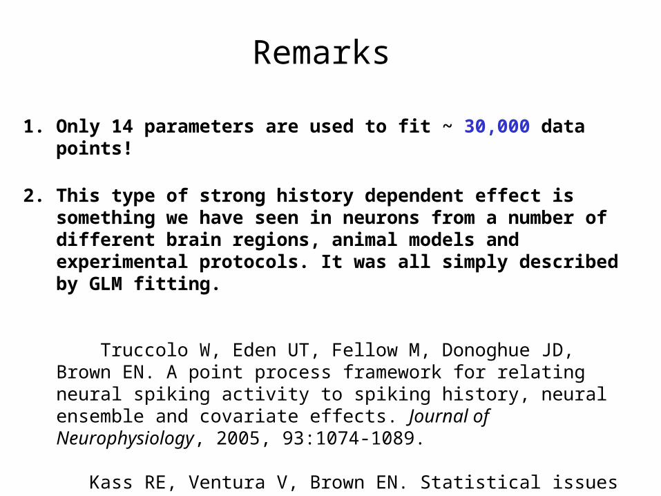
Remarks

1. Only 14 parameters are used to fit ~ 30,000 data points!

2. This type of strong history dependent effect is something we have seen in neurons from a number of different brain regions, animal models and experimental protocols. It was all simply described by GLM fitting.

Truccolo W, Eden UT, Fellow M, Donoghue JD, Brown EN. A point process framework for relating neural spiking activity to spiking history, neural ensemble and covariate effects. Journal of Neurophysiology, 2005, 93:1074-1089.

Kass RE, Ventura V, Brown EN. Statistical issues in the analysis of neuronal data. Journal of Neurophysiology, 2005, 94: 8-25.

Case 2: An Analysis of the Spiking Activity of STN Neurons in Parkinson Patients and Healthy Primate

The spiking activity of sub-thalamic neurons of basal ganglia in Parkinson patients and healthy primate is recorded under identical experimental conditions. Subjects execute a center-out directed hand-movement task.

*Sarma, Cheng, Eden, Hu, Williams, Brown, Eskandar, 2008

Sub-Thalamic Nucleus

Neurophysiological Data

Single Neuronal Recordings from STN

0

1

time

1 Primate96 Neurons868 trials

8 Patients3-15 neurons/patient24-470 trials/patient

Behavioral Task

Grey ArrayAppears

500-1000 ms

Target cue

500-1000 ms

“U”

“R”

“D”

“L”

Go cue

500-1000 ms

Fixation

500 ms

Move

“U”

“R”

“D”

“L”

Reach & Hold

100 ms

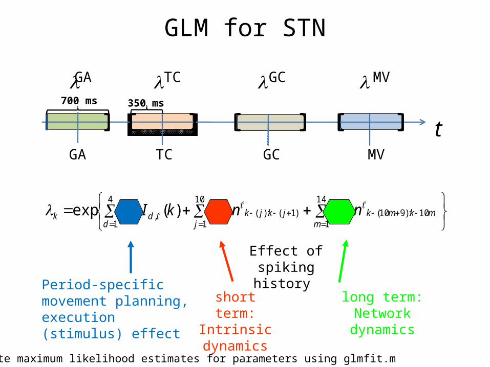
TC GC MV

t350 ms

GA

700 ms

GA TC GC MV

mkmk

mmjkjk

jj

dddk nnkI 10:)910(

14

1,)1(:)(

10

1,

4

1,, )(exp

Effect of spiking history

long term:Network

dynamics

Period-specific movement planning, execution (stimulus) effect

GLM for STN

Compute maximum likelihood estimates for parameters using glmfit.m

short term:Intrinsic

dynamics

KS Plots of PD Models

GLM Coefficient Estimates

PD Model Primate Model

HEALTHY PRIMATE PD PATIENT

50 Hz

50% oscillations (10-30 Hz)

40% bursting

8% directionalselectivity

35% directionalselectivity

30 Hz

15% oscillations (10-30 Hz)

12% bursting

250 msec 250 msec

rate function

spike train

0.35

“Parkinsonian” Motor Symptoms akinesia/bradykinesia

resting tremor

rigidity

“Parkinsonian” STN Neural Symptoms 10-30 Hz oscillations

bursting

directional selectivity

lower firing rate

Population Summary

Summary

• GLM provides a computationally tractable generalization of the Gaussian linear model to non-Gaussian regression models.

• Estimation is carried out using maximum likelihood. This analysis has all the properties of maximum likelihood.

• AIC, deviance and parameter standard errors provide measures of goodness-of-fit and an inference framework analogous to regression.

• Can be applied to other exponential family models.

• Non-canonical link functions can also be used.

• GLM is a standard tool in Matlab, Minitab, R, S, SAS, Splus, and SPSS.

Acknowledgments

We are grateful to Julie Scott for technical assistance.

Reference

McCullagh P, Nelder JA. Generalized Linear Model, 2nd Edition. Chapman and Hall, 1989.