2011 NSF-CMACS Workshop on Atrial Fibrillation (3rd day ) · 2011 NSF-CMACS Workshop on Atrial...
48
2011 NSF-CMACS Workshop on Atrial Fibrillation (3 rd day ) Flavio H. Fenton Department of Biomedical Sciences College of Veterinary Medicine, Cornell University, NY and Max Planck Institute for Dynamics and Self-organization, Goettingen, Germany Lehman College, Bronx, NY. Jan 3-7, 2011
Transcript of 2011 NSF-CMACS Workshop on Atrial Fibrillation (3rd day ) · 2011 NSF-CMACS Workshop on Atrial...

2011 NSF-CMACS Workshop on
Atrial Fibrillation (3rd day )
Flavio H. Fenton
Department of Biomedical Sciences
College of Veterinary Medicine,
Cornell University, NY
and
Max Planck Institute for Dynamics and
Self-organization, Goettingen, Germany
Lehman College,
Bronx, NY. Jan 3-7, 2011

Transition from Sinus Rhythm to Fibrillation
Normal Rhythm VT VF
Sudden
cardiac death
Cherry EM, Fenton FH, Am J Physiol 2004; 286: H2332
Cherry EM, Fenton FH, New J. Phys. 2008; 10, 125016

Spiral Waves in the Heart
How can we know they are there?
How can we see them?

Visualizing Electrical Activity in Cardiac Tissue

Optical Mapping
Visualizing Electrical Activity in Cardiac Tissue
Tissue
bath
Tissue is kept alive by perfusion

Optical Mapping
• Di-4-ANEPPS (voltage-sensitive dye)
Voltage = changes in fluorescence
• Diodes: 530 nm wavelength
• Cascade cameras at 511 Hz
• 128x128 window view
Visualizing Electrical Activity in Cardiac Tissue

Fluorescence Imaging with di-4-ANNEPS
Intensity AND maximum of spectrum change with membrane potential.
Fractional intensity change 1-10% (for a filter cut-off of λ = 600 nm)
Excitation wavelength
Emission wavelength

Optical Mapping Setup
Dual camera
setting

Example of Action Potential
Recordings in Ventricular Tissue
Optical mapping
Microelectrode
Recordings:
Better signal-to-noise
Discontinuous in space
Not for long times
-85mV
20mV

Normal Sinus Rhythm
Plane Waves (Optical Mapping)
Electrical activity in the atria Electrical activity in the
ventricle
20mV
-85mV

Cherry EM, Fenton FH. New Journal of Physics 2008; 10: 125016
Spiral Waves:Simulations and Optical Mapping
Anatomical
reentry

Circular core
spiral waveLinear core
spiral wave
Cherry EM, Fenton FH. New Journal of Physics 2008; 10: 125016
Spiral Waves:Simulations and Optical Mapping
Anatomical
reentry

Different Types of Arrhythmias
• Ventricular Fibrillation
Spiral waves are complicated
The dynamics of multiple spiral waves
is not simple, with multiple short lived.
Spiral Wave Instabilities
From one spiral to multiple spirals?
How to prevent?
How to terminate?
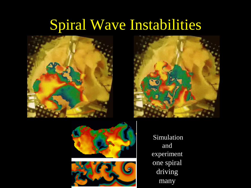
Spiral Wave Instabilities
Simulation
and
experiment
one spiral
driving
many

In Reality, the Heart Is a 3D System

Dual-Surface Optical Mapping
In Reality, the Heart Is a 3D System

Dual-Surface Optical Mapping
In Reality, the Heart Is a 3D System

2D 3D
Spiral waves Scroll waves
spiral tip vortex filament
How to Visualize Reentry in 3D?

Similar to water spouts
How to Visualize Reentry in 3D?

How to Visualize Reentry in 3D?

Continuous Rotational AnisotropyFiber rotation induces a phase on the wave fronts
between layers, producing a localized twist along
the filament.
Twist propagation

How to Visualize Reentry in 3D?

Ventricular Fibrillation in 3D

Enough introductionHow do we model cell and cardiac dynamics?
The study of cardiac arrhythmias from a computational point of view
started in 1946 in Mexico.
N. Wiener and A. Rosenblueth, ‘‘The mathematical formulation of the
problem of conduction of impulses in a network of connected excitable
elements, specifically in cardiac muscle,’’ Arch. Inst. Cardiol. Mex 16,
205–265. 1946
Arturo
Rosenblueth
The best model for a cat is another cat,
Preferable the same cat.
Norbert
Wiener
Fathers of Cybernetics

Enough introductionThe first mathematical model of electrical AP
J. Physiol. Vol 117 500-540, 1952 by
A.L. Hodgkin and A.F. Huxley.

Ca2+, Na+, K+
Electrical Activity in Myocites

The Hodgkin-Huxley model of four variables for neurons
J. Physiol. Vol 117 500-540, 1952 by
A.L. Hodgkin and A.F. Huxley.
How to model the Neuron AP?
Capacitance is a measure of the amount of electrical energy stored
(or separated) for a given electric potential, where C = Q/V
Q_m = CV_m ; dQ_m/dt = I_ion; Therefore I_ion = C dV_m/dt
dV_m/dt = I_ion/C

The Hodgkin-Huxley model of four variables for neurons
Cell currents
for the model
(follow Ohms law)
Ecuaciones para la
probabilidad de las
puertas
J. Physiol. Vol 117 500-540, 1952 by
A.L. Hodgkin and A.F. Huxley.
How to model the Neuron AP mathematically?

Gating Variables• Gating variables are time-dependent variables
that modify the current conductance.
• Gates vary between 0 and 1; 1 maximizes current and 0 eliminates it.
• Gates follow the following equation:
where y∞(V) is the steady-state value and τy(V) is the time constant for the gate.
y
yy
t
y
d
d

The Hodgkin-Huxley model of four variables for neurons
Cell currents
for the model
(follow Ohms law)
Ecuaciones para la
probabilidad de las
puertas
J. Physiol. Vol 117 500-540, 1952 by
A.L. Hodgkin and A.F. Huxley.
How to model the Neuron AP mathematically?

Hodgkin-Huxley four variable model
How to model the Neuron AP mathematically?
http://thevirtualheart.org/java/neu
ron/apneuron.html

S2 30,17.6 17.5
13
IS2 -300, -350
-450
N, gna 70, 40
Change Rest
Membrane p.
N t=80, gna =
180, 188, 200,
300
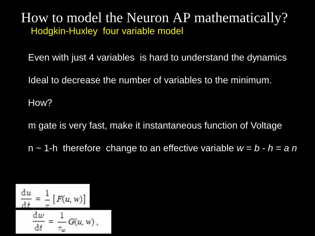
How to model the Neuron AP mathematically?Hodgkin-Huxley four variable model
http://thevirtualheart.org/java/neu
ron/apneuron.html

Even with just 4 variables is hard to understand the dynamics
Ideal to decrease the number of variables to the minimum.
How?
m gate is very fast, make it instantaneous function of Voltage
n ~ 1-h therefore change to an effective variable w = b - h = a n
How to model the Neuron AP mathematically?Hodgkin-Huxley four variable model
How to model the Neuron AP mathematically?Hodgkin-Huxley four variable model
Even with just 4 variables is hard to understand the dynamics
Ideal to decrease the number of variables to the minimum.
How?
m gate is very fast, make it instantaneous function of Voltage
n ~ 1-h therefore change to an effective variable w = b - h = a n

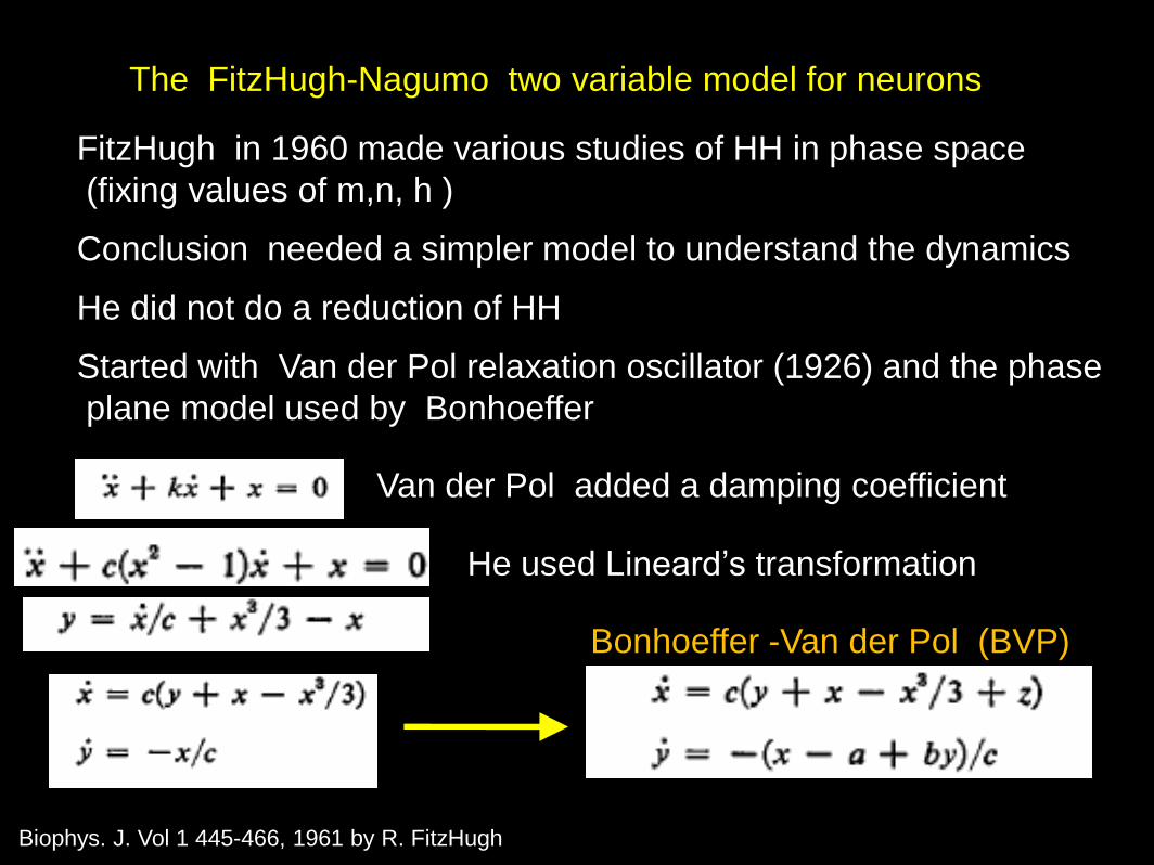
The FitzHugh-Nagumo two variable model for neurons
Biophys. J. Vol 1 445-466, 1961 by R. FitzHugh
Biophys. J. Vol 1 445-466, 1961 by R. FitzHugh
FitzHugh in 1960 made various studies of HH in phase space
(fixing values of m,n, h )
Conclusion needed a simpler model to understand the dynamics
He did not do a reduction of HH
Started with Van der Pol relaxation oscillator (1926) and the phase
plane model used by Bonhoeffer
Van der Pol added a damping coefficient
He used Lineard’s transformation
Bonhoeffer -Van der Pol (BVP)
The FitzHugh-Nagumo two variable model for neurons

Biophys. J. Vol 1 445-466, 1961 by R. FitzHugh
Four floor to ceiling relay racks,
With vacuum tubes (that failed around twice a week)
And overloaded the air conditining
The FitzHugh-Nagumo two variable model for neurons

Biophys. J. Vol 1 445-466, 1961 by R. FitzHugh
The FitzHugh-Nagumo two variable model for neurons
http://thevirtualheart.org
/java/fhn24.html

Nullclines and phase space analysis

Biophys. J. Vol 1 445-466, 1961 by R. FitzHugh
Phase space:
a .1 .2 .3 .4
.5
Delta .2,.1.5,1.
Eps .01 .02
.03 .04
Eps .01 .005 .002
.001
The FitzHugh-Nagumo two variable model for neurons
http://thevirtualheart.org/java/fh
nphase.html

Biophys. J. Vol 1 445-466, 1961 by R. FitzHugh
S2 10,9,8,7
a .1 .2 .3 .4
.5
Delta
.2,.1.5,1.
Also by
a =-.1
S2 =0
Eps .01 .02
.03 .04
Eps .01
.005 .002
.001
S2 larger
Eps .0001
T 700
S2 464 463
T2000
S2 600,
900 1000
1500 Dynamics of FHN model > 2 h class
The FitzHugh-Nagumo two variable model for neurons
http://thevirtualheart.org/java/fhn25.html

Cell models
(for different animals and cell types)

Early Models
Examples:
• Noble model (1964) (first cardiac model, based on HH model)
4 variables. 3 currents.
• Beeler-Reuter (1977), Luo-Rudy 1 (1991) 8 vaiables.
• Primary currents:– INa: responsible for upstroke
– ICa: responsible for plateau
– IK: time-dependent and time-independent components responsible for repolarization
– Background currents to balance things out (masking unknowns).

Modeling Cellular Electrophysiology
has become more and more complex
Getting very complex:
87 ode + others for stress activated ion channels + contraction equations

Models, Models Everywhere
• Surge in development of models of cardiac myocyte EP over the last 5-10 years.
• 37 models included on Cell ML website through 2004 (not inclusive)
• ~1/3 in most recent 3 years.
• Multiple models for same species/region.
Cardiac EP Models
1960-1969
1970-1979
1980-1989
1990-1994
1995-1997
1998
1999
2000
2001
2002
2003
2004
2004
1995-1997
1960s
20001999
1970s
1990-1994
1980s
20011998
2002
2003
Number of Cardiac EP Models
37 Total Cell ML Site
Java applets of 45 different cardiac EP models at scholarpedia (models of cardiac cell)
Google : cell models scholarpedia

Many Models for Different Cell Types and animals
Implemented most (~40) of the published models in single cells and in tissue.