2010 Winter School on Machine Learning and Vision Sponsored by Canadian Institute for Advanced...
95
2010 Winter School on Machine Learning and Vision Sponsored by Canadian Institute for Advanced Research and Microsoft Research India With additional support from Indian Institute of Science, Bangalore and The University of Toronto,
-
Upload
leroy-arendale -
Category
Documents
-
view
214 -
download
0
Transcript of 2010 Winter School on Machine Learning and Vision Sponsored by Canadian Institute for Advanced...

2010 Winter School on Machine Learning and Vision
Sponsored byCanadian Institute for Advanced
Researchand Microsoft Research India
With additional support from
Indian Institute of Science, Bangaloreand The University of Toronto, Canada
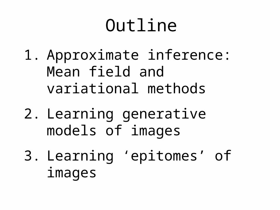
Outline
1. Approximate inference: Mean field and variational methods
2. Learning generative models of images
3. Learning ‘epitomes’ of images
Part AApproximate inference: Mean field
and variational methods

Line processes for binary images (Geman and Geman 1984)
0 00 0
Function, fPatterns with high f
1 10 0
0 01 1
1 01 0
0 10 1
1 11 1
1 00 0
Patterns with low f0 10 0
0 01 0
0 00 1
0 11 1
1 01 1
1 10 1
1 11 0
Under P, “lines”are probable
1 00 1
0 11 0
Use tablet to derive variational inference method

Denoising images using line process models

Part BLearning Generative Models of Images
Brendan Frey
University of Toronto and
Canadian Institute for Advanced Research

Generative models
• Generative models are trained to explain many different aspects of the input image– Using an objective function like log P(image), a
generative model benefits by account for all pixels in the image
• Contrast to discriminative models trained in a supervised fashion (eg, object recognition)– Using an objective function like log P(class|image),
a discriminative model benefits by accounting for pixel features that distinguish between classes

What constitutes an “image”
• Uniform 2-D array of color pixels
• Uniform 2-D array of grey-scale pixels
• Non-uniform images (eg, retinal images, compressed sampling images)
• Features extracted from the image (eg, SIFT features)
• Subsets of image pixels selected by the model (must be careful to represent universe)
• …

What constitutes a generative model?

Learning Bayesian Networks:Exact and approximate methods

Maximum likelihood learning when all variables are visible (complete data)
• Suppose we observe N IID training cases v(1)…v(N)
• Let q be the parameters of a model P(v)
• Maximum likelihood estimate of q:
qML = argmaxq Pn P(v(n)|q)
= argmaxq log( Pn P(v(n)|q) )
= argmaxq Sn log P(v(n)|q)

Complete data in Bayes nets
• All variables are observed, so P(v|q) = PiP(vi|pai,qi)
where pai = parents of vi, qi parameterizes P(vi|pai)
• Since argmax () = argmax log (),
qiML = argmaxqi
Sn log P(v(n)|q)
= argmaxqi Sn Si log P(vi
(n)|pai(n),qi)
= argmaxqi Sn log P(vi
(n)|pai(n),qi)
Each child-parent module can be learned separately

Example: Learning a Mixture of Gaussians from labeled data
• Recall: For cluster k, the probability density of x is
The probability of cluster k is p(zk = 1) = pk
• Complete data: Each training case is a (zn,xn) pair, let
Nk be the number of cases in class k
• ML estimation: ,
That is, just learn one Gaussian for
each class of data

Example: Learning from complete data, a continuous child with continuous parents
• Estimation becomes a regression-type problem
• Eg, linear Gaussian model:
P(vi|pai,qi) = N (vi; wi0+Sn:onpaiwinvn,Ci),
• mean = linear function of parents
• Estimation: Linear regression

Learning fully-observed MRFs
• It turns out we can NOT directly estimate each potential using only observations of its variables
• P(v|q) = Piϕ(vCi|qi) / (SvPiϕ(vCi
|qi))
• Problem: The partition function (denominator)

Learning Bayesian networks when there is missing data
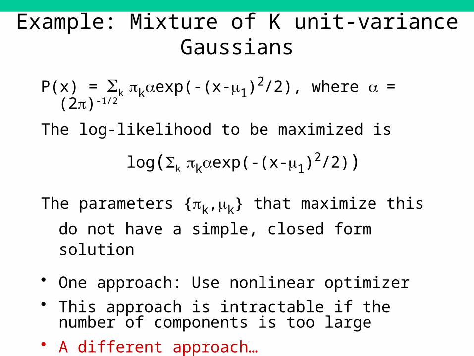
Example: Mixture of K unit-variance Gaussians
P(x) = Sk pkaexp(-(x-m1)2/2), where a = (2p)-1/2
The log-likelihood to be maximized is
log(Sk pkaexp(-(x-m1)2/2))
The parameters {pk,mk} that maximize this do not have a
simple, closed form solution
• One approach: Use nonlinear optimizer• This approach is intractable if the number of
components is too large• A different approach…

The expectation maximization (EM) algorithm(Dempster, Laird and Rubin 1977)
• Learning was more straightforward when the data was complete
• Can we use probabilistic inference (compute P(h|v,q)) to “fill in” the missing data and then use the learning rules for complete data?
• YES: This is called the EM algorithm

• Initialize q (randomly or cleverly)
• E-Step: Compute Q(n)(h) = P(h|v(n),q) for hidden variables
h, given visible variables v
• M-Step: Holding Q(n)(h) constant, maximize
Sn ShQ(n)(h) log P(v(n),h|q)
wrt q
• Repeat E and M steps until convergence
• Each iteration increases log P(v|q) = Sn log(ShP(v,h|q))
Expectation maximization (EM) algorithm
“Ensemble completion”
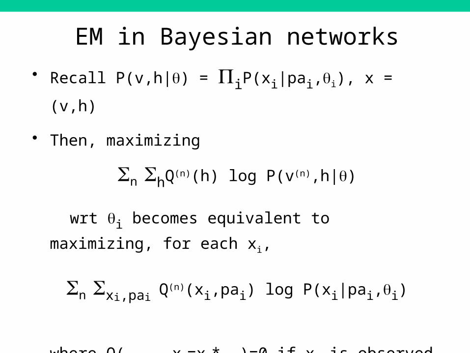
• Recall P(v,h|q) = PiP(xi|pai,qi), x = (v,h)
• Then, maximizing
Sn ShQ(n)(h) log P(v(n),h|q)
wrt qi becomes equivalent to maximizing, for each xi,
Sn Sxi,pai Q(n)(xi,pai) log P(xi|pai,qi)
where Q(..., xk=xk*,…)=0 if xk is observed to be xk*
• GIVEN the Q-distributions, the conditional P-distributions can be updated independently
EM in Bayesian networks

• E-Step: Compute Q(n)(xi,pai) = P(xi,pai|v(n),q) for each
variable xi
• M-Step: For each xi, maximize
Sn Sxi,pai Q(n)(xi,pai) log P(xi|pai,qi)
wrt qi
EM in Bayesian networks

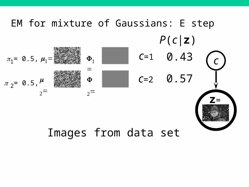
EM for a mixture of Gaussians• Initialization: Pick m’s, S’s, p ’s randomly but validly
• E Step: For each training case, we need
q(z) = p(z|x) = p(x|z)p(z) / (Sz p(x|z)p(z))
Defining = q(znk=1), we need to actually compute:
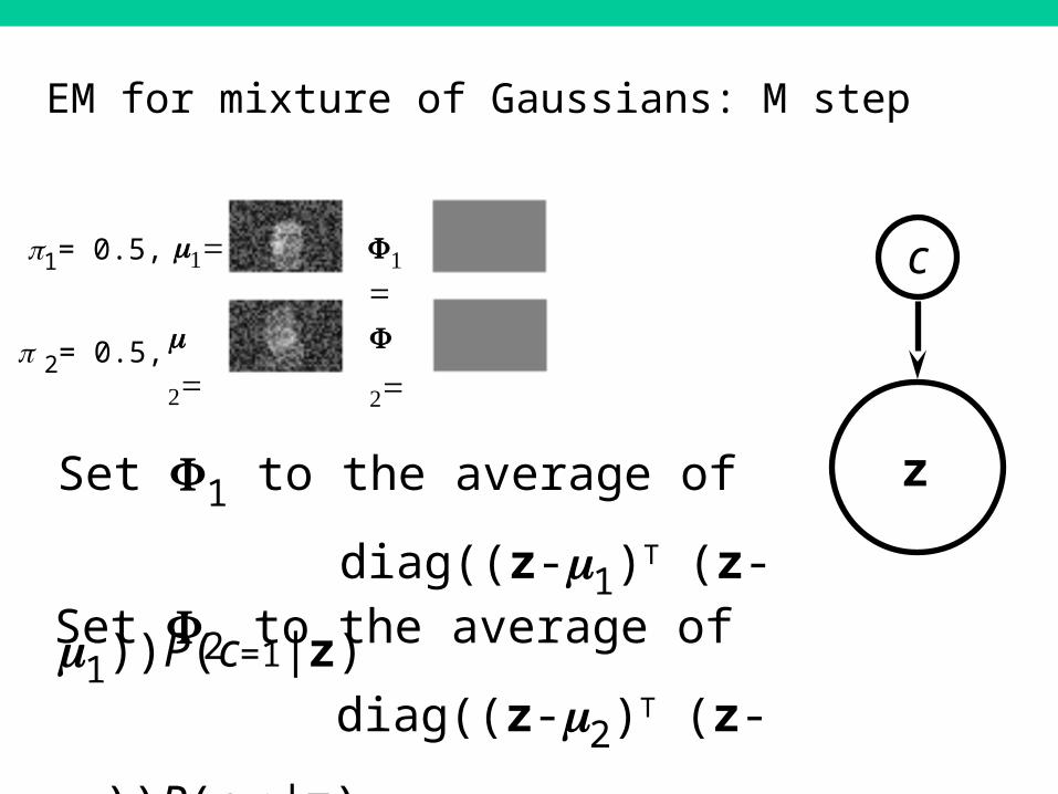
• M Step:
Do it in the log-domain!
Recall: For labeled data, g(znk)=znk

EM for mixture of Gaussians: E step
c
z
m1=
F1=
m
2=
F
2=
p1= 0.5,
p 2= 0.5,
Images from data set
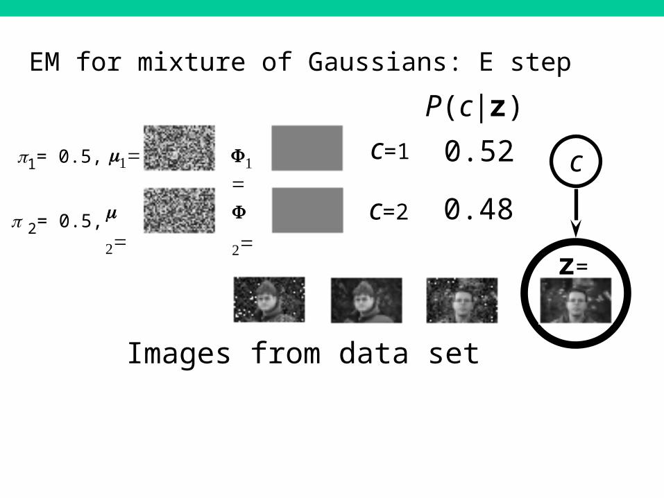
c=1
Images from data set
z=
c=2
P(c|z)
c0.52
0.48
m1=
F1=
m
2=
F
2=
p1= 0.5,
p 2= 0.5,
EM for mixture of Gaussians: E step

Images from data set
z=
cc=1
c=2
P(c|z)
0.51
0.49
m1=
F1=
m
2=
F
2=
p1= 0.5,
p 2= 0.5,
EM for mixture of Gaussians: E step

Images from data set
z=
cc=1
c=2
P(c|z)
0.48
0.52
m1=
F1=
m
2=
F
2=
p1= 0.5,
p 2= 0.5,
EM for mixture of Gaussians: E step
Images from data set
z=
cc=1
c=2
P(c|z)
0.43
0.57
m1=
F1=
m
2=
F
2=
p1= 0.5,
p 2= 0.5,
EM for mixture of Gaussians: E step

cm1=
F1=
m
2=
F
2=
p1= 0.5,
p 2= 0.5,
zSet m1 to the average of zP(c=1|
z)Set m2 to the average of zP(c=2|
z)
EM for mixture of Gaussians: M step

cm1=
F1=
m
2=
F
2=
p1= 0.5,
p 2= 0.5,
zSet m1 to the average of zP(c=1|
z)Set m2 to the average of zP(c=2|
z)
EM for mixture of Gaussians: M step
cm1=
F1=
m
2=
F
2=
p1= 0.5,
p 2= 0.5,
zSet F1 to the average of
diag((z-m1)T (z-m1))P(c=1|z)Set F2 to the average of
diag((z-m2)T (z-m2))P(c=2|z)
EM for mixture of Gaussians: M step

cm1=
F1=
m
2=
F
2=
p1= 0.5,
p 2= 0.5,
zSet F1 to the average of
diag((z-m1)T (z-m1))P(c=1|z)Set F2 to the average of
diag((z-m2)T (z-m2))P(c=2|z)
EM for mixture of Gaussians: M step
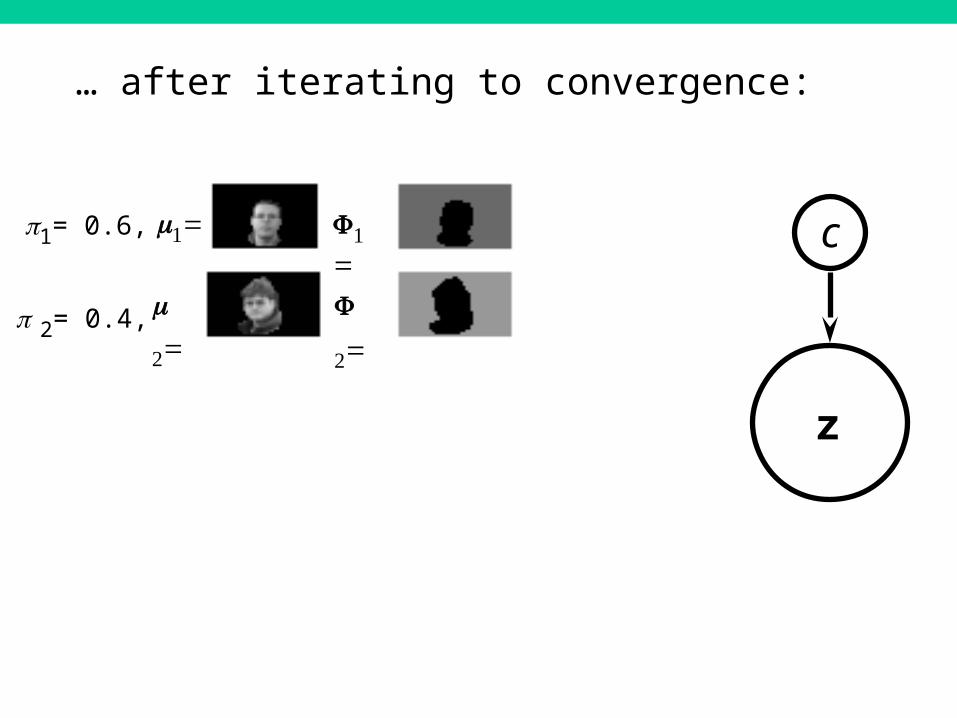
… after iterating to convergence:
c
z
m1=
F1=
m
2=
F
2=
p1= 0.6,
p 2= 0.4,

Why does EM work?

Gibbs free energy• Somehow, we need to move the log() function in
the expression log(ShP(h,v)) inside the
summation to obtain log P(h,v), which simplifies
• We can do this using Jensen’s inequality:
log ( ) log( ( ))h
P v P h v ( )
log( ( ) )( )h
P h vQ h
Q h
( )( ) log( ) ( )
( )h
P h vQ h F Q P
Q h
Free energy
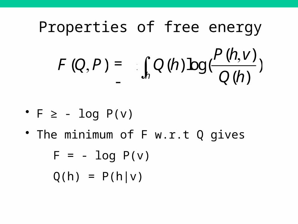
Properties of free energy
• F ≥ - log P(v)
• The minimum of F w.r.t Q gives
F = - log P(v)
Q(h) = P(h|v)
( )( ) log( ) ( )
( )h
P h vQ h F Q P
Q h
( )( ) log( ) ( )
( )h
P h vQ h F Q P
Q h
= -

Proof that EM maximizes log P(v)(Neal and Hinton 1993)
• E-Step: By setting Q(h)=P(h|v), we make the bound tight, so that F = - log P(v)
• M-Step: By maximizing Sh Q(h) logP(h,v) wrt the
parameters of P, we are minimizing F wrt the parameters of P
Since -log Pnew(v) ≤ Fnew ≤ Fold = -log Pold(v), we have log Pnew(v) ≥ log Pold(v). ☐
( )( ) log( ) ( )
( )h
P h vQ h F Q P
Q h
( )( ) log( ) ( )
( )h
P h vQ h F Q P
Q h
= -
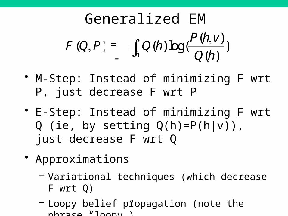
Generalized EM
• M-Step: Instead of minimizing F wrt P, just decrease F wrt P
• E-Step: Instead of minimizing F wrt Q (ie, by setting Q(h)=P(h|v)), just decrease F wrt Q
• Approximations– Variational techniques (which decrease F wrt Q)
– Loopy belief propagation (note the phrase “loopy”)
– Markov chain Monte Carlo (stochastic …)
( )( ) log( ) ( )
( )h
P h vQ h F Q P
Q h
( )( ) log( ) ( )
( )h
P h vQ h F Q P
Q h
= -
Summary of learning Bayesian networks
• Observed variables decouple learning in different conditional PDFs
• In contrast, hidden variables couple learning in different conditional PDFs
• Learning models with hidden variables entails iteratively filling in hidden variables using exact or approximate probabilistic inference, and updating every child-parent conditional PDF

Back to…Learning Generative Models of Images
Brendan Frey
University of Toronto and
Canadian Institute for Advanced Research

What constitutes an “image”
• Uniform 2-D array of color pixels
• Uniform 2-D array of grey-scale pixels
• Non-uniform images (eg, retinal images, compressed sampling images)
• Features extracted from the image (eg, SIFT features)
• Subsets of image pixels selected by the model (must be careful to represent universe)
• …
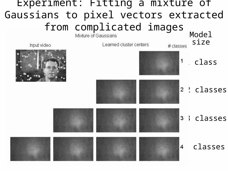
Modelsize
1 class
2 classes
3 classes
4 classes
Experiment: Fitting a mixture of Gaussians to pixel vectors extracted from complicated images

Why didn’t it work?
• Is there a bug in the software?– I don’t think so, because the log-likelihood
monotonically increases and the software works properly for toy data generated from a mixture of Gaussians
• Is there a mistake in our mathematical derivation?– The EM algorithm for a mixture of Gaussians has
been studied by many people – I think the math is ok

Why didn’t it work?
• Are we missing some important hidden variables?
• YES: The location of each object
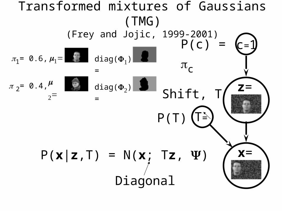
x
z
TT=
cc=1P(c) = pc
P(x|z,T) = N(x; Tz, Y)
m1=
diag(F1) =
m
2=
p1= 0.6,
p 2= 0.4,Shift, T
P(T)
diag(F2) = z=
x=
Diagonal
Transformed mixtures of Gaussians (TMG)(Frey and Jojic, 1999-2001)

EM for TMG
x
T
c
z
• E step: Compute Q(T)=P(T|x), Q(c)=P(c|x), Q(c,z)=P(z,c|x) and Q(T,z)=P(z,T|x) for each x in data
• M step: Set
– pc = avg of Q(c)
– rT = avg of Q(T)
– mc = avg mean of z under Q(z|c)
– Fc = avg variance of z under Q(z|c)
– Y = avg var of x-Tz under Q(T,z)
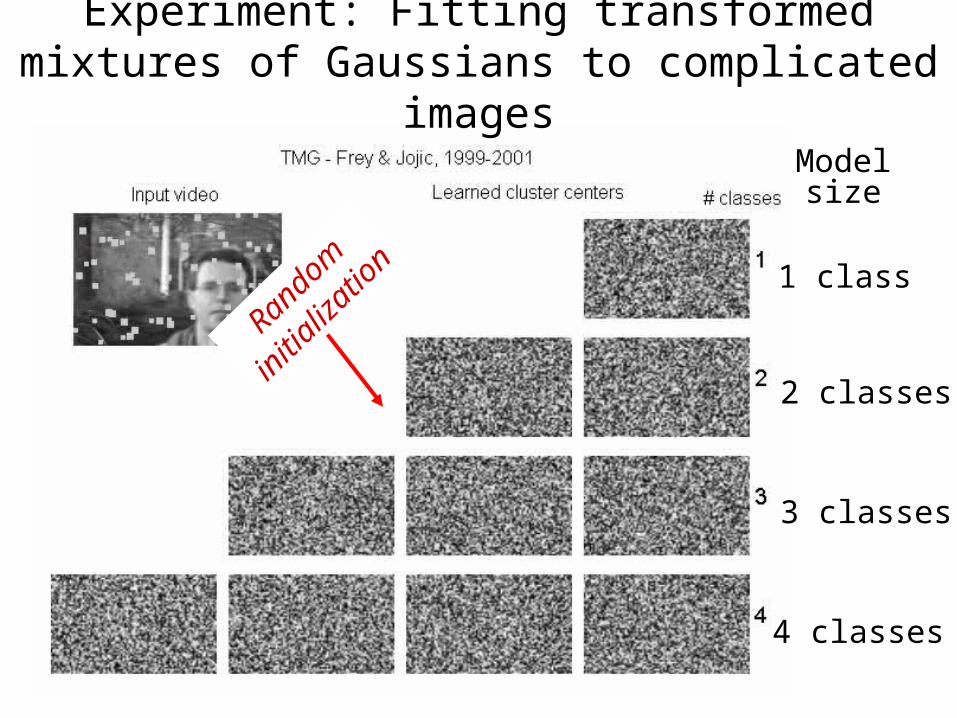
Modelsize
1 class
2 classes
3 classes
4 classes
Random
initialization
Experiment: Fitting transformed mixtures of Gaussians to complicated images
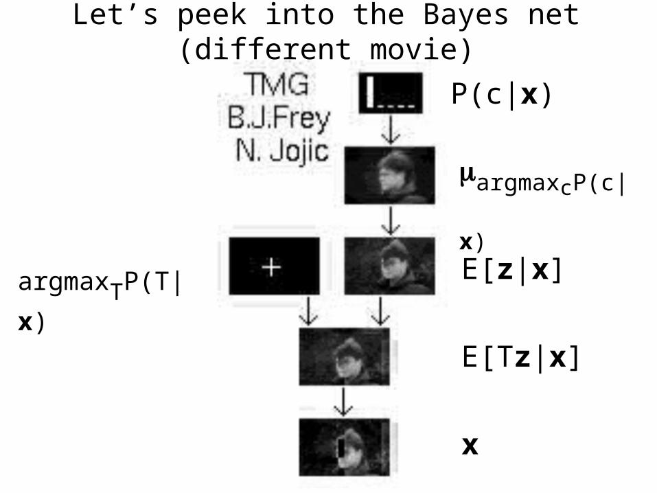
Let’s peek into the Bayes net (different movie)
E[z|x]
P(c|x)
margmaxcP(c|x)
argmaxTP(T|x)
E[Tz|x]
x

tmgEM.m is available on the web

Accounting for multiple objects in the same image

How can we compose an image that includes multiple objects?
• In TMG, the foreground and background were distinguished by the noise map
• When there are multiple objects, we need a way to assign each pixel to one object
m1=
diag(F1) =
m
2=
p1= 0.6,
p 2= 0.4, diag(F2) =

Layered 2.5-D representations
• Adelson and Anandan (1990) described image patches as a composition of 2-D layers:
Image = mask x foreground picture
+ (1-mask) x background picture

=
•( • +
• )
• +
Example
•

A generative model for layered vision(Jojic and Frey 2001, Frey, Kannan and Jojic, 2003)

Movies

A generative model for layered vision(Jojic and Frey 2001, Frey, Kannan and Jojic, 2003)

Random variables• Appearance and transparency of layer l: ,• Class of layer l:• Contribution that layer l makes to the input:
• Transformation of layer l:• Contribution of layer l, including transformations:
• Subspace coordinate, layer l:• Image
s m
1
1( (1 ))ii
m m s
T
1
1( (1 ))i ii
Tm Tm T s
z
c
1
11
( (( (1 )) ) )L
i ii
N
x Tm Tm T s

Probability model
• Image model:
• Model of hidden variables:
• Joint pdf:
1( { } )Lp x s m T 1
11
( (( (1 )) ) )L
i ii
N
x Tm Tm T s
( ) ( )
( ) ( 0 )
s s sc c c c
m m mc c c
p c N
N N
Ts m T z s z
m z z I
1
11
( { } )
( { } ) ( )
L
LL
p c
p p c
x s m T z
x s m T s m T z
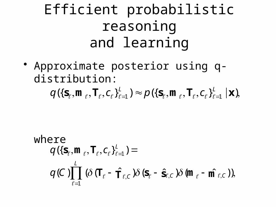
Efficient probabilistic reasoningand learning
• Approximate posterior using q-distribution:
where
1 1({ } ) ({ } )L Lq c p c s m T s m T x
1
1
({ } )
ˆ( ) ( ( ) ( ) ( ))ˆ ˆ
L
L
CCC
q c
q C
s m T
T s ms mT

Optimizing q
• Minimize the variational free energy:
• Algorithm:– Initialize variational parameters
– Select a variational parameter or a model parameter, and adjust it so as to minimize F
– Repeat until convergence
( )( ) log
( )
( )( ) log log ( ) log ( )
( )
h
h
q hF q h
p h v
q hq h p v p v
p h v

Inference updates
• Q(c) update:
• Introduce auxiliary variables:
• Rewriting the image model:
1ˆ( ) ( { } )ˆ ˆ LCC Cq C p C x s m T
1 1 1 11 1
1 1
1 1
(1 ) ˆ
ˆ
ji i j j j ji j
Lj
L j j j jj
Tm Tm T sm x m
mTm T sx
m
1
1 1 1
( { } )
( ( (1 ) ) )ˆ ˆ
L
k k k Lk k k k k k
p
N
x s m T
x T m T s T mx m x
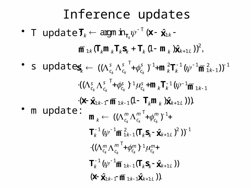
• T update:
• s update:
• m update:
Inference updatesT
1
21 1
(argmin ˆ
( (1 ) ))ˆ
kkk
k k Lk k k k k k
TT x x
T m T s T mm xT 1 2 1 1 12
1 1
T 1 1 11 1
1 1 1 1 1
(( ) ( ))
(( ) (
( (1 ) )))ˆ ˆ
kk k
k k kk
ss skck c c k k
ss s sc c c k k kc
k k k Lk k
s m T m
m T m
x T mx m xT 1
1 1 2 121 1 1
T 1
1 11 1 1
1 1 1 1 1
(( )
( ( ) ))ˆ
(( )
( ( ))ˆ
( ))ˆ ˆ
kk k
k k kk
mm mck c c
k k Lk k k
mm m mc c cc
k k Lk k k
k k k L
m
T T sm x
T T sm x
x x m x

Learning updates
• Image variances:
• Other params:
1( { } )Lp x s m T 1
11
( (( (1 )) ) )L
i ii
N
x Tm Tm T s
( ) ( )
( ) ( 0 )
s s sc c c c
m m mc c c
p c N
N N
Ts m T z s z
m z z I


Movies
Inferring leg motion

Accounting for local image features using ‘epitomes’
• A good way to model local image features is to factorize them (cf Bruno’s talk)
• A simpler method is to cluster them (Freeman and Pasztor, 1999)
• A generative model based on clustered image patches needs a way to account for how image patches are coordinated

Learning the ‘epitome’ of an image(Jojic, Kannan and Frey, ICCV 2003)

Movies

An EM-type learning algorithm

Gaussian likelihood model
Patch k
Map fromepitome to
image
Set of pixelindices inpatch k
Epitome(parameters)
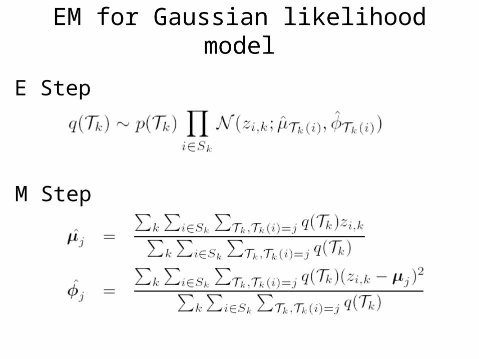
EM for Gaussian likelihood model
M Step
E Step

Examples

Examples
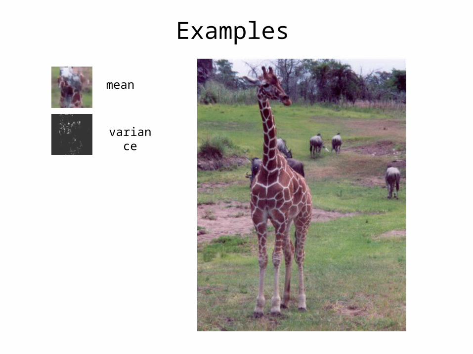
Examples
mean
variance

Why epitomes are interesting & useful• Generative model of multi-sized patches
• Invariant to transformations (eg, affine)
• Organizes and compresses patch data
• Proximity of patches in epitome probability patches belong to same ‘part’
• Incomplete observations are stitched into a single model
• Can model patterns at a wide range of scales
• Searching an epitome is much faster than searching an ‘equivalent’ library of patches

Applications
• Data compression
• Data summarization and user interface
• Denoising
• Parts-based image modeling
• Segmentation
• …

Application: Image editing
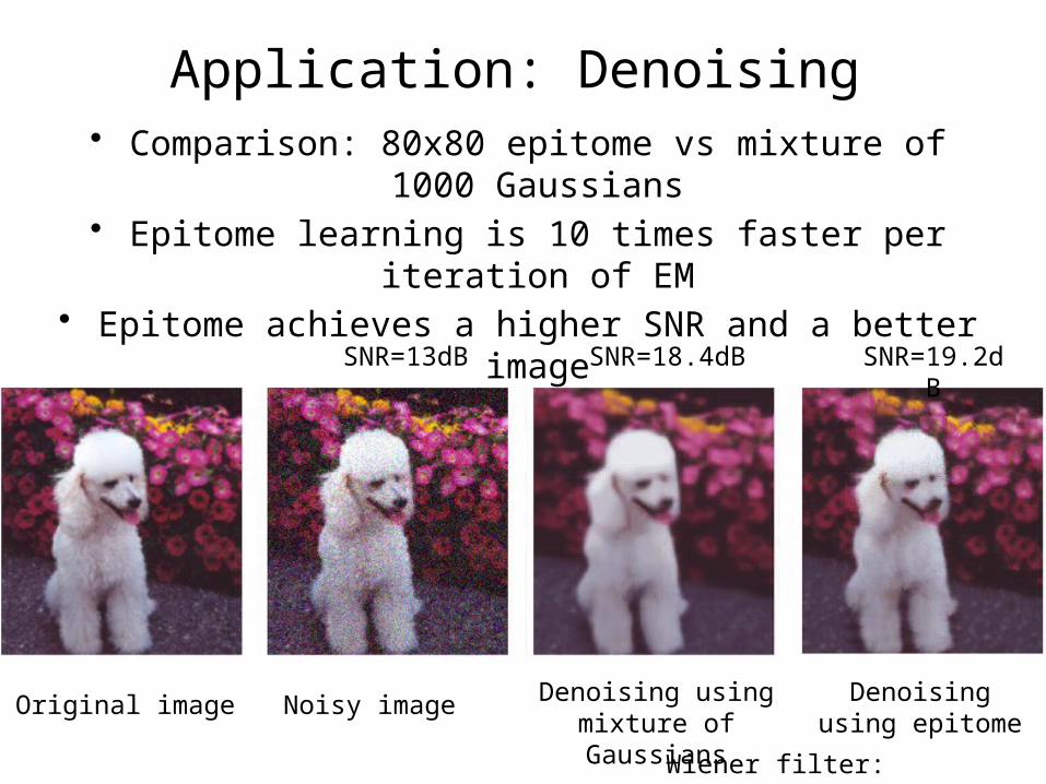
Application: Denoising
Original image Noisy image Denoising using mixture of Gaussians
Denoising using epitome
SNR=13dB SNR=18.4dB SNR=19.2dB
Wiener filter: 16.1dB
• Comparison: 80x80 epitome vs mixture of 1000 Gaussians• Epitome learning is 10 times faster per iteration of EM• Epitome achieves a higher SNR and a better image

Using epitomes to model images with multiple parts
EmEs
S1 S2 M
X
X=M*S1+(1-M)*S2 + noise
appearance
epitome
shape
epitome
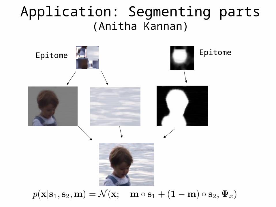
Application: Segmenting parts(Anitha Kannan)
em
es
S1 s2 M
x
Epitome Epitome

Joint distribution and inference
Exact inference is intractable, so we minimize the free energy using a variational method:
Variational approximation to posterior

Parameterizing the approximation to the posterior
Delta Dirac
Estimated value for all patches
containing i
Idea: We should fit the relaxed model under the constraint that the generative patches
agree in the overlapping regions

The bound simplifies
Posterior
Bound
For this q function, the bound simplifies into a sum of quadratic terms than can be efficiently optimized by a generalized EM
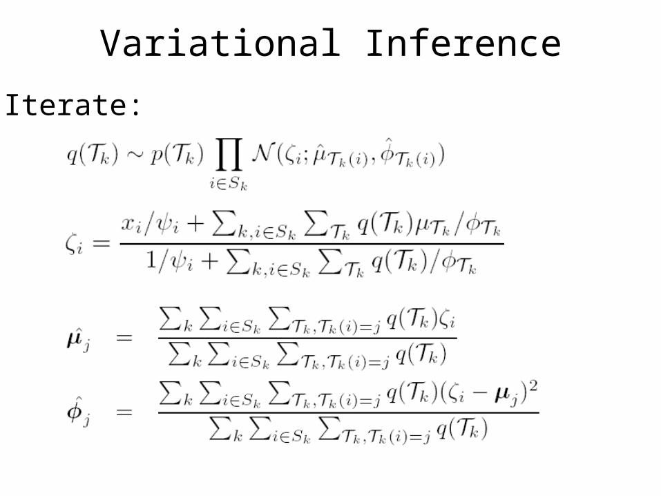
Variational Inference
Iterate:

Application: Segmenting parts
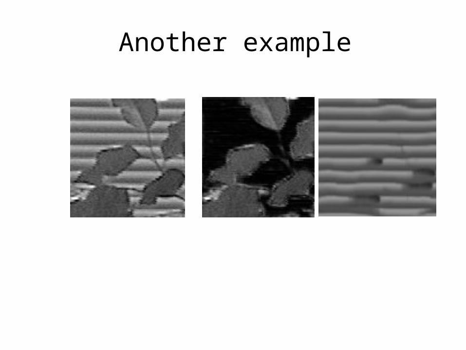
Another example
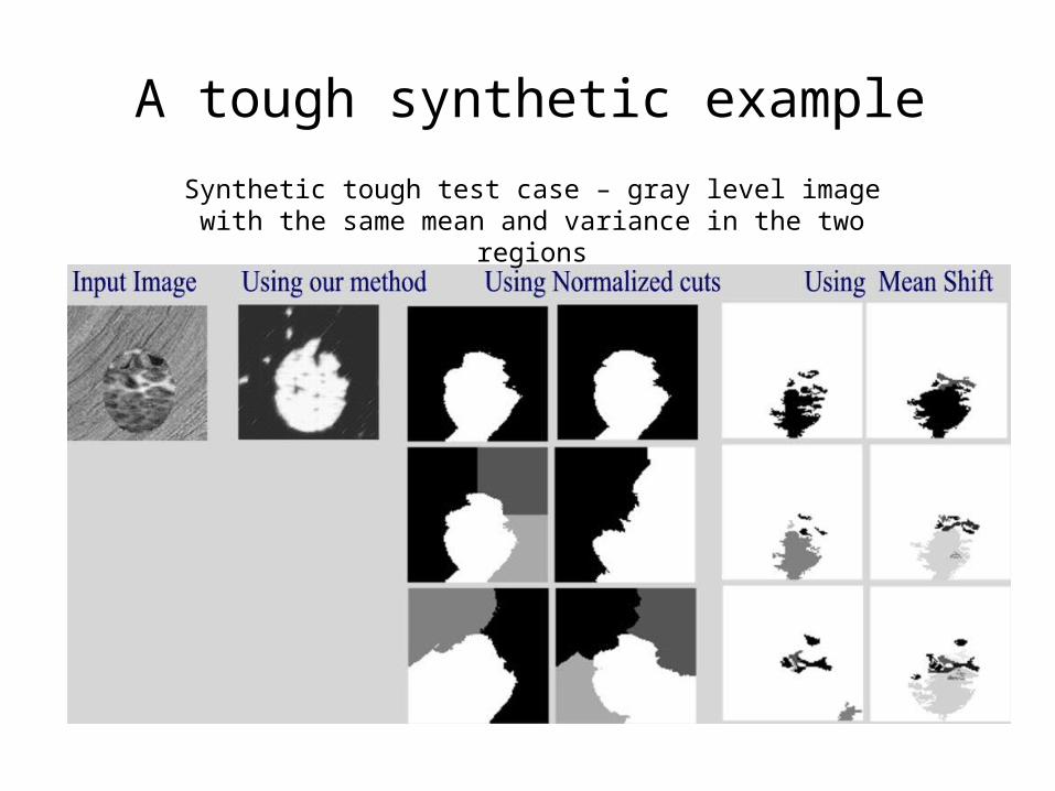
A tough synthetic example
Synthetic tough test case – gray level image with the same mean and variance in the two regions
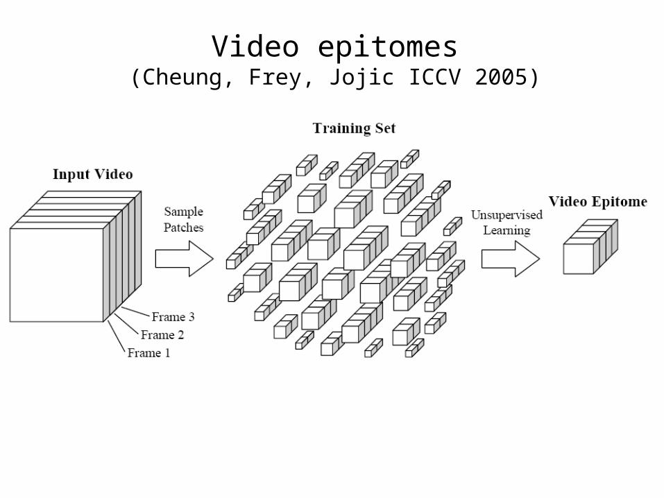
Video epitomes(Cheung, Frey, Jojic ICCV 2005)

Examples of video epitomes
Temporally compressed epitome
Spatially compressed epitome

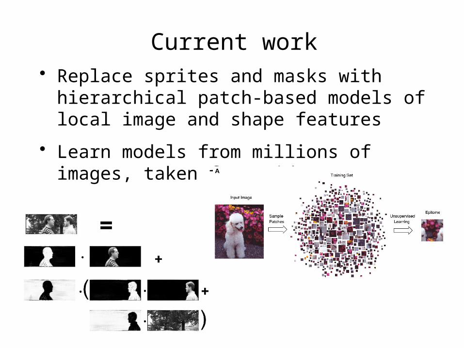
Current work• Replace sprites and masks with hierarchical
patch-based models of local image and shape features
• Learn models from millions of images, taken from videos

Summary
• Generative models are trained to explain many different aspects of the input image– Using an objective function like log P(image), a
generative model benefits by account for all pixels in the image
• Contrast to discriminative models trained in a supervised fashion (eg, object recognition)– Using an objective function like log P(class|image),
a discriminative model benefits by accounting for pixel features that distinguish between classes

Rejecting a common criticism of generative models
• Critics of generative models often point to well-defined tasks (eg, object recognition) and claim that discriminatively trained classifiers (eg, SVMs) perform better
• I would argue that these tasks are often not representative of real-world problems– Hand-written digit recognition
– Identifying cows in PASCAL or Caltech256 images
– Classifying gene function using microarray data

Accepting a common criticism of generative models
• On specific supervised learning tasks, discriminative methods (eg, SVMs) usually perform better
Current work• Replace sprites and masks with hierarchical
patch-based models of local image and shape features
• Learn models from millions of images, taken from videos