WORKING DRAFT

Fluvial Sediment Transport as an Overlay to Instream Flow Recommendations for the Environmental Flows Allocation Process

Senate Bill 3 Science Advisory Committee for Environmental Flows

Document Version Date: March 20, 2009

Report # SAC-2009-0X

WORKING DRAFT

TABLE OF CONTENTS SECTION 1 FLUVIAL SEDIMENT TRANSPORT ................................................................ 1 SECTION 2 PURPOSE AND SCOPE........................................................................................ 3 SECTION 3 RATIONALE AND CONTEXT............................................................................ 4 

3.1  TEXAS SENATE BILL 2................................................................................................. 4 3.2  TEXAS SENATE BILL 3................................................................................................. 4 

SECTION 4 METHODS OF ASSESSMENT ............................................................................ 6 4.1  HISTORICAL SUSPENDED-SEDIMENT DATA ......................................................... 6 4.2  HISTORICAL BEDLOAD DATA ................................................................................... 7 4.3  SEDIMENT TRANSPORT MODELS ............................................................................. 8 4.4  EFFECTIVE DISCHARGE .............................................................................................. 9 

SECTION 5 RECOMMENDATIONS AND EXAMPLE COMPUTATION OF EFFECTIVE DISCHARGE ...................................................................................................... 12 

5.1  EXAMPLE OF EFFECTIVE DISCHARGE ANALYSIS ............................................. 12 5.1.1  Flow-Duration Curve ................................................................................................ 14 5.1.2  Suspended-Sediment Load........................................................................................ 15 5.1.3  Cross-Sectional Data................................................................................................. 17 5.1.4  Bagnold’s (1977) Bedload Model............................................................................. 19 

5.2  ADVOCACY OF THE SAM HYDRAULC DESIGN MODEL.................................... 22 SECTION 6 DECISION POINTS............................................................................................. 23 SECTION 7 CONCLUSIONS ................................................................................................... 26 SECTION 8 REFERENCES...................................................................................................... 27 SECTION 9 GLOSSARY........................................................................................................... 30 SECTION 10 CONTRIBUTORS .............................................................................................. 31 

WORKING DRAFT

LIST OF TABLES Table 1. Data required for effective discharge analysis at 08114000 Brazos River at Richmond, Texas ..............................................................................................................................................14 Table 2. Computations for the flow-duration curve and histogram for determination of effective discharge for suspended-sediment load .........................................................................................17 Table 3. Computations for bedload transport using the Bagnold (1977) model and effective discharge for bedload.....................................................................................................................20

WORKING DRAFT

LIST OF FIGURES Figure 1. Conceptual diagram of a large fluvial system, with an emphasis on sediment erosion transport, and deposition..................................................................................................................1 Figure 2. Generalized mechanisms of fluvial transport ..................................................................2 Figure 3. Type-I hysteresis loop of suspended-sediment concentrations for two stormflow events ...............................................................................................................................................6 Figure 4. Effective discharge in its graphical form.........................................................................9 Figure 5. Effective discharge in this example approximately is equal to the bankfull discharge.10 Figure 6. Concepts of equilibrium in fluvial geomorphology ......................................................11 Figure 7. Procedural flowchart for recommended computation of effective discharge for suspended-sediment load, bedload, and total load.........................................................................13 Figure 8. Flow-duration curve for 08114000 Brazos River at Richmond, Texas.........................14 Figure 9. Suspended-sediment-load and streamflow rating curve for 08114000 Brazos River at Richmond, Texas ...........................................................................................................................15 Figure 10. Suspended-sediment load (SSL) histogram showing effective discharge for SSL at 08114000 Brazos River at Richmond, Texas ................................................................................16 Figure 11. Cross section of 08114000 Brazos River at Richmond, Texas ...................................18 Figure 12. Bedload histogram showing an inaccurately low estimate of effective discharge for bedload at 08114000 Brazos River at Richmond, Texas...............................................................21

WORKING DRAFT

SECTION 1 FLUVIAL SEDIMENT TRANSPORT

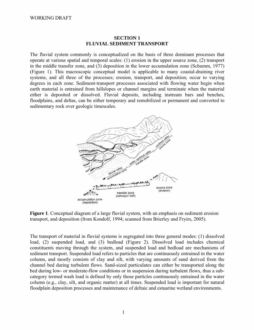
The fluvial system commonly is conceptualized on the basis of three dominant processes that operate at various spatial and temporal scales: (1) erosion in the upper source zone, (2) transport in the middle transfer zone, and (3) deposition in the lower accumulation zone (Schumm, 1977) (Figure 1). This macroscopic conceptual model is applicable to many coastal-draining river systems, and all three of the processes; erosion, transport, and deposition; occur to varying degrees in each zone. Sediment-transport processes associated with flowing water begin when earth material is entrained from hillslopes or channel margins and terminate when the material either is deposited or dissolved. Fluvial deposits, including instream bars and benches, floodplains, and deltas, can be either temporary and remobilized or permanent and converted to sedimentary rock over geologic timescales.

Figure 1. Conceptual diagram of a large fluvial system, with an emphasis on sediment erosion transport, and deposition (from Kondolf, 1994; scanned from Brierley and Fryirs, 2005). The transport of material in fluvial systems is segregated into three general modes: (1) dissolved load, (2) suspended load, and (3) bedload (Figure 2). Dissolved load includes chemical constituents moving through the system, and suspended load and bedload are mechanisms of sediment transport. Suspended load refers to particles that are continuously entrained in the water column, and mostly consists of clay and silt, with varying amounts of sand derived from the channel bed during turbulent flows. Sand-sized particulates can either be transported along the bed during low- or moderate-flow conditions or in suspension during turbulent flows, thus a sub-category termed wash load is defined by only those particles continuously entrained in the water column (e.g., clay, silt, and organic matter) at all times. Suspended load is important for natural floodplain deposition processes and maintenance of deltaic and estuarine wetland environments.

1

WORKING DRAFT

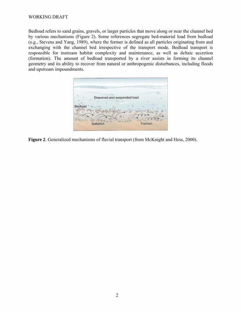
Bedload refers to sand grains, gravels, or larger particles that move along or near the channel bed by various mechanisms (Figure 2). Some references segregate bed-material load from bedload (e.g., Stevens and Yang, 1989), where the former is defined as all particles originating from and exchanging with the channel bed irrespective of the transport mode. Bedload transport is responsible for instream habitat complexity and maintenance, as well as deltaic accretion (formation). The amount of bedload transported by a river assists in forming its channel geometry and its ability to recover from natural or anthropogenic disturbances, including floods and upstream impoundments.

Figure 2. Generalized mechanisms of fluvial transport (from McKnight and Hess, 2000).

2

WORKING DRAFT

3

SECTION 2 PURPOSE AND SCOPE

This report provides guidance for the inclusion of fluvial sediment transport as a possible overlay to the HEFR approach for determination of an environmental flow regime required by Texas Senate Bill 3 (Senate Bill 3 Science Advisory Committee for Environmental Flows, 2009). Although numerous sources associate the majority of fluvial sediment transport with high-pulse flows, the discussion and guidance provided below are not contingent on an exclusive association of sediment transport with HEFR-based high-pulse flows. In many cases, a healthy sediment regime could be associated either with overbank, high-pulse, or even base flows. Further, it should be recognized that sediment transport processes do not encompass the full breadth of fluvial geomorphic investigation, but can be readily associated with an environmental flow regime. Section 3 of this report provides a rationale and context to justify inclusion of a sediment transport overlay to the environmental flows allocation process mandated by Texas Senate Bill 3. Section 4 discusses various methods of assessment, including the use of historical data, model equations, and computation of effective discharge. Further, strengths and weaknesses of various methods are presented. Section 5 recommends the effective discharge approach to assess sediment transport at gaging stations and briefly discusses some limitations of this approach. Further, a step-by-step example of the effective discharge approach at a long-term USGS streamflow-gaging station is provided and the use of the SAM hydraulic design model for estimation of effective discharge is advocated. Section 6 identifies several decision points that a practitioner tasked with a sediment-transport analysis will encounter. Section 7 draws some general conclusions and reinforces various limitations of an effective discharge analysis. This report originally was prepared by the Science Advisory Committee, with comments from the Texas Water Development Board (TWDB). Members of the Science Advisory Committee have reviewed, edited, and expanded the document and have provided recommendations regarding the application of the information and procedures presented in the document pursuant to the requirements of SB 3.

WORKING DRAFT

SECTION 3 RATIONALE AND CONTEXT

As flows increase from base flow to high-pulse flows to overbank floods, rates of sediment transport in the water column and at the channel bed greatly increase. The erosion, transport, and deposition of sediment are as important to the complexity and structural diversity of rivers, riparian zones, deltas, and estuaries as the conveyance of water itself. The balance between the force of water and the resistance of sediment sculpts the many fluvial patterns and shapes that provide habitats and conditions to which aquatic and riparian species uniquely adapt over time. If only flows are considered, without the associated sediment, then an incomplete assessment of the state’s rivers and bays reduces the likelihood of conservation or rehabilitation. A worst-case scenario might involve high-pulse flow releases that increase rates of habitat degradation.

3.1 TEXAS SENATE BILL 2

The importance of sediment and river channel morphology has been highlighted by instream-flow activities associated with Texas Senate Bill 2. Also, in a National Research Council review of the Texas Instream Flow Program (TIFP) (2005), it was stated that the section considering physical processes and sediment required “significant augmentation” to relate them to the hydrologic regime, and that a “thin, single set of analytical approaches” would be insufficient to “address the range or complexity of physical processes.” In response to these comments, the state agencies responsible for the TIFP further addressed physical processes and sediment in the revised technical overview document (TOD) of the TIFP (2008), which contains the following statements: “Geomorphic studies will assess the active channel processes responsible for developing

physical habitats.” “Agencies will develop sediment budgets…” “…geomorphic studies need to be tailored to the specific sub-basin being investigated” “…the lack of geomorphic data for Texas’ rivers is problematic.” “…a monitoring program that collects geomorphic data for major rivers will be

required.” The TOD goes on to recommend specific lines of inquiry to address these problems and achieve program goals.

3.2 TEXAS SENATE BILL 3

Texas Senate Bill 3 mandates that locally based basin and bay expert science teams (BBESTs), with consultations and support from the Environmental Flows Science Advisory

4

WORKING DRAFT

5

Committee (SAC) and basin and bay area stakeholder committees, “develop environmental flow analyses and a recommended flow regime” that “maintain(s) the viability of the state’s streams, rivers, and bay and estuary systems” using “reasonably available science.” BBESTs are responsible for flow recommendations required by Senate Bill 3. It is thus within their purview to consider reasonably available scientific methods to account for instream sediment and its delivery to bay and estuary systems. The imminent deadlines for which the BBESTs must provide flow-regime recommendations exclude the possibility of making present-day sediment-load measurements and analyses for the short-term requirements. However, estimates or predictions of sediment transport for various flows would serve as a benchmark from which to assess programmatic goals, and adaptive management practices could include consideration of sediment data as they become available.

Measurable objectives that link sediment to healthy rivers and floodplains include achieving optimized: (1) channel-bed elevations and rates of bank erosion; (2) instream geomorphic unit structure and function, including composition and adjustment frequency of units such as pool-riffle sequences, bars, and benches, among others (see Brierley and Fryirs, 2005); (3) turbidity; and (4) floodplain accretion rates. Measureable objectives that link sediment to healthy estuaries include achieving optimized: (1) rates of deltaic accretion, (2) rates of estuarine shoreline erosion, and (3) turbidity. Achieving these objectives would promote healthy aquatic and riparian habitats by supporting the abiotic conditions to which native species have successfully adapted over time.

WORKING DRAFT

SECTION 4 METHODS OF ASSESSMENT

Suspended load and bedload are measured or estimated separately because the physical processes that govern their rates of transport are contingent on different factors. The sum of suspended load and bedload is the total sediment load. Methods to assess suspended load and bedload in Texas rivers and streams can be separated into two categories: (1) historical data analyses and (2) model estimates.

4.1 HISTORICAL SUSPENDED-SEDIMENT DATA

Historical suspended-sediment load data are available until the early 1980s for various streamflow-gaging stations in Texas, and are derived from two general sources: (1) reports published by the Texas Water Development Board (TWDB) and predecessor agencies and (2) the U.S. Geological Survey (USGS). Suspended-sediment load measurements commonly are associated with discharge to generate a sediment-discharge rating curve. This, however, is problematic because suspended-sediment concentrations are known to be variable for a given discharge. Stormflow hydrographs usually, but not always, are characterized by higher suspended-sediment concentrations during the rising limb than the falling limb, referred to as a type-I hysteresis loop (Figure 3). Further, the timing between storm events also influences availability of sediment from the watershed, such that an initial stormflow following relatively dry conditions usually has a greater suspended-sediment concentration than subsequent flows of similar magnitude. Aside from these complications, assessments of suspended-sediment load for various flows are encouraged.

Figure 3. Type-I hysteresis loop of suspended-sediment concentrations for two stormflow events, showing (1) concentrations higher on the rising limb than the falling limb and (2) sediment exhaustion effects for the second, larger flood (from Hudson, 2003). A series of reports by the TWDB and predecessor agencies (Stout et al., 1961; Adey and Cook, 1964; Cook, 1967; Cook, 1970; Mirabal, 1974; Dougherty, 1979; Quincy, 1988) summarize daily suspended-sediment concentration and load measurements into monthly values at various

6

WORKING DRAFT

stations in Texas over various periods of record. The data were collected by the “Texas-sampler method”. Historic suspended sediment samples were obtained in an 8-oz narrow-neck bottle held in a 10-lb torpedo-shaped frame, positioned no more than one foot below the water surface. Samples were obtained daily at one-sixth, one-half, and five-sixths of the water-surface width (Stout et al., 1961). To account for increasing suspended sediment concentrations with depth, the measured percent of suspended sediment by weight was multiplied by 1.102 to obtain the mean percentage of suspended sediment in the vertical profile (Quincy, 1988). The data summarized in these reports were collected to estimate reservoir siltation and should be used with caution for determining an environmental flow regime. The USGS also collected suspended-load data at various stations in Texas and for various periods of record. Data typically were collected 5 to 10 times per year for various flow magnitudes. The data can be accessed through the National Water Information System (NWIS) at http://waterdata.usgs.gov/tx/nwis/qwdata. USGS suspended-sediment data were collected by one of two methods: (1) equal-discharge-increment (EDI) or (2) equal-width-increment (EWI) (Edwards and Glysson, 1999). In simple terms, the EDI method obtains depth-integrated samples of suspended sediment from the centroids of equal-discharge increments across the channel. The EWI method obtains depth-integrated samples of suspended sediment at equally-spaced increments across the channel. Both methods provide similarly accurate results. A comparison of the “Texas-sampler method” and the USGS method was made by Welborn (1967). For sand-bed rivers, including the Sabine, Neches, Trinity, and San Jacinto, correlations could not be formulated between the two methods and preference is given to the more accurate USGS method because of highly-variable ratios of the two estimates along different rivers. However, for rivers with mixed or gravel beds, it was found that suspended-sediment load (in tons/year) computed by the former method closely matches loads computed by the USGS method. Strengths: representative of historical conditions; measured data; easily coupled with streamflow measurements Weaknesses: USGS data not available since mid-1990s; TWDB data not available since mid-1980s; Texas-sampler method not as accurate as USGS depth-integrated method; restricted to selected streamflow-gaging stations; restricted to the measurement period of record

4.2 HISTORICAL BEDLOAD DATA

Historical bedload data for Texas rivers are practically unavailable. Discrete measurements of bedload probably are available in isolated sources associated with one-time investigations. However, the great difficulties in accurately measuring bedload, especially in sand-bed channels, should be considered if data sources are located. If sufficient historical bedload data are identified and their quality deemed acceptable, then computations of effective discharge for bedload transport can be made with available streamflow data. Strengths: representative of historical conditions; measured data

7

WORKING DRAFT

Weaknesses: mostly unavailable, unless embedded within published or unpublished project-specific reports; restricted to measurement stations; restricted to the measurement period of record

4.3 SEDIMENT TRANSPORT MODELS

Bedload models, usually based on hydraulic principles, are notoriously inaccurate (Gomez and Church, 1989), uncertain (Gomez and Phillips, 1999), and applicable to rivers that exhibit steady-state equilibrium, but offer the most rapid approach to estimate transport. The various formulas for estimating bedload transport commonly require values for bed-material particle size, channel slope (energy gradient), flow depth, among other measureable or estimated factors. Common bedload transport equations include Meyer-Peter and Müller (1948), Einstein (1950), Ackers and White (1973), Bagnold (1980), Parker et al. (1982), and Gomez (2006), among others. The choice of bedload equations should be based on: (1) the composition of the bed material, (2) channel geometry, and (3) the hydraulic conditions under consideration. If changes in channel-bed and bank positions over time are known, another approach is Exner’s equation used in a morphodynamic model. The following sources provide useful bedload transport model equations and explanations: (1) Gomez and Church (1989), (2) Stevens and Yang (1989), and (3) Robert (2003). A very useful application to estimate bedload and suspended-load transport is SAM – Hydraulic Design Package for Channels, which includes various sediment transport equations that accompany a one-dimensional hydraulic computation model. User input to SAM includes channel cross-sectional data, energy gradient (channel slope), bed-material particle size distributions, and a roughness value, among other limited data. The SAM application assesses the user input to determine which sediment transport equations are most applicable, and then computes sediment transport loads using a combination of model output with the cross-sectional geometry data. Further, flow-duration curve data can be included to determine which flows cumulatively transport the most sediment over time, referred to as the effective discharge. A final comment should be made that personnel involved with application of sediment transport models or SAM should have considerable background or training, and caution should be given to computed estimates. For some rivers in Texas, a source of data to parameterize sediment-transport models is provided in a 4-CD set of data published by the National Cooperative Highway Research Program (2004). Further, cross-sectional data from streamflow measurements can be requested from the U.S. Geological Survey (USGS) water-science centers in Texas. Strengths: not contingent on sediment-load measurements; flexibility over space and time (e.g., model parameters could be from any station along a river, or could be historical) Weaknesses: result accuracy; requires accurate model parameters (e.g., cross-sectional data, channel slope, bed-material size distribution)

8

WORKING DRAFT

4.4 EFFECTIVE DISCHARGE

Sediment load is a measure of mass transport over time and, with a reasonably extensive dataset, one could formulate sediment-flow prescriptions in the same manner as streamflow. However, the most commonly applied method to associate sediment load with streamflow is through an analysis of effective discharge. Effective discharge is the flow that cumulatively transports the majority of sediment at a channel cross section over time (Figure 4). It is usually a flow of moderate magnitude and frequency. Although high-magnitude floods can transport substantial quantities of sediment, their relatively infrequent occurrence often is outpaced by the sediment transport of more frequent moderate flows. Although effective discharge is informative with respect to sediment transport, it offers little guidance in predicting channel form or adjustment over time.

Figure 4. Effective discharge, in its graphical form, is the largest product of the sediment transport rate and the frequency of transport (from Wolman and Miller, 1960; scanned from Andrews and Nankervis, 1998). Although a number of investigations confirm that relatively frequent, moderate flows (Hudson and Mossa, 1997) or bankfull flows (Andrews and Nankervis, 1995; Biedenharn et al., 1999; Torizzo and Pitlick, 2004) are responsible for the majority of cumulative sediment transport over time (Figure 5), others have shown that infrequent, high-magnitude floods equate to the effective discharge (Gupta, 1988; Bourke and Pickup, 1999), especially in fluvial systems with highly variable flow regimes. Generally, effective discharge is less frequent as the average annual precipitation and regularity of flooding decreases. A further complication associated with applications of effective discharge is the tendency to rely solely on one flow value to transport sediment over time. Instead, an emphasis on flow variability and the range of flows necessary to transport sediment over time should be embraced. For example, average flow conditions are known to transport appreciable quantities of sediment in sand-bed river systems.

9

WORKING DRAFT

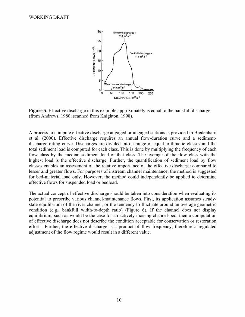
Figure 5. Effective discharge in this example approximately is equal to the bankfull discharge (from Andrews, 1980; scanned from Knighton, 1998). A process to compute effective discharge at gaged or ungaged stations is provided in Biedenharn et al. (2000). Effective discharge requires an annual flow-duration curve and a sediment-discharge rating curve. Discharges are divided into a range of equal arithmetic classes and the total sediment load is computed for each class. This is done by multiplying the frequency of each flow class by the median sediment load of that class. The average of the flow class with the highest load is the effective discharge. Further, the quantification of sediment load by flow classes enables an assessment of the relative importance of the effective discharge compared to lesser and greater flows. For purposes of instream channel maintenance, the method is suggested for bed-material load only. However, the method could independently be applied to determine effective flows for suspended load or bedload. The actual concept of effective discharge should be taken into consideration when evaluating its potential to prescribe various channel-maintenance flows. First, its application assumes steady-state equilibrium of the river channel, or the tendency to fluctuate around an average geometric condition (e.g., bankfull width-to-depth ratio) (Figure 6). If the channel does not display equilibrium, such as would be the case for an actively incising channel-bed, then a computation of effective discharge does not describe the condition acceptable for conservation or restoration efforts. Further, the effective discharge is a product of flow frequency; therefore a regulated adjustment of the flow regime would result in a different value.

10

WORKING DRAFT

Figure 6. Concepts of equilibrium in fluvial geomorphology (from Schumm, 1977; scanned from Ritter et al., 2002). Channel rehabilitation or engineering applications focus on graded time scales, and efforts are usually made to promote a steady-state channel condition that is resilient to disturbances (e.g., floods). Strengths: adaptable to both measured and model-estimated data; adaptable to bedload, suspended-load, or total load Weaknesses: assumes steady-state equilibrium; restricted to streamflow-measurement stations; restricted to the streamflow-measurement period of record

11

WORKING DRAFT

SECTION 5 RECOMMENDATIONS AND EXAMPLE COMPUTATION OF EFFECTIVE

DISCHARGE

An analysis of the effective discharge of sediment transport at gaging stations with a sufficient period of record (20 or more years) could serve as an overlay to modify HEFR-based flow prescriptions (mostly high-pulse flows or overbank flows). For gaging stations with accurate suspended-load data, effective discharge can be computed using the methodology described in Biedenharn et al. (2000). Bedload transport can be accounted for with a model equation, which requires inputs of bed-material size, channel slope, cross-sectional geometry, and flow depth, among other hydraulically relevant parameters. The caveat of using measured suspended-load data is that the values represent conditions during the period of measurement, which might have been degraded or not representative of desired conditions for many rivers in Texas, especially for stations downstream of reservoirs. It should be recognized that an analysis of effective discharge does not encompass nor entirely explain the breadth of fluvial geomorphic processes. Sediment transport, however, is a fairly straightforward process to relate with streamflow, and collection of sediment-transport data commonly occurs simultaneous with streamflow at a gaging station.

5.1 EXAMPLE OF EFFECTIVE DISCHARGE ANALYSIS

An illustrative example is provided below for the Brazos River near Richmond, Texas, using streamflow and suspended-load data from the USGS National Water Information System (NWISWeb) (U.S. Geological Survey, 2009) and supporting data from the National Cooperative Highway Research Program (2004). Further, a procedural flowchart of effective discharge analysis is shown in Figure 7. Data required for an analysis of effective discharge at 08114000 Brazos River at Richmond, Texas, are summarized in Table 1.

12

WORKING DRAFT

Figure 7. Procedural flowchart for recommended computation of effective discharge for suspended-sediment load, bedload, and total load.

13

WORKING DRAFT

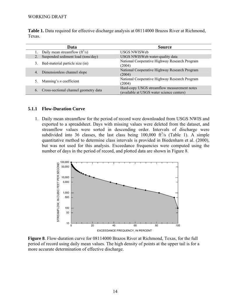
Table 1. Data required for effective discharge analysis at 08114000 Brazos River at Richmond, Texas.

Data Source 1. Daily mean streamflow (ft3/s) USGS NWISWeb 2. Suspended sediment load (tons/day) USGS NWISWeb water-quality data

3. Bed-material particle size (in) National Cooperative Highway Research Program (2004)

4. Dimensionless channel slope National Cooperative Highway Research Program (2004)

5. Manning’s n coefficient National Cooperative Highway Research Program (2004)

6. Cross-sectional channel geometry data Hard-copy USGS streamflow measurement notes (available at USGS water science centers)

5.1.1 Flow-Duration Curve

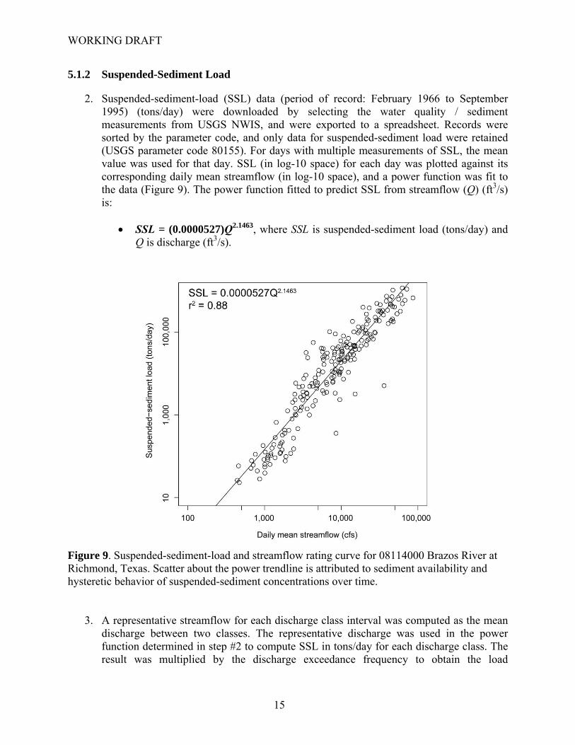
1. Daily mean streamflow for the period of record were downloaded from USGS NWIS and exported to a spreadsheet. Days with missing values were deleted from the dataset, and streamflow values were sorted in descending order. Intervals of discharge were subdivided into 36 classes, the last class being 100,000 ft3/s (Table 1). A simple quantitative method to determine class intervals is provided in Biedenharn et al. (2000), but was not used for this analysis. Exceedance frequencies were computed using the number of days in the period of record, and plotted data are shown in Figure 8.

Figure 8. Flow-duration curve for 08114000 Brazos River at Richmond, Texas, for the full period of record using daily mean values. The high density of points at the upper tail is for a more accurate determination of effective discharge.

14

WORKING DRAFT

5.1.2 Suspended-Sediment Load

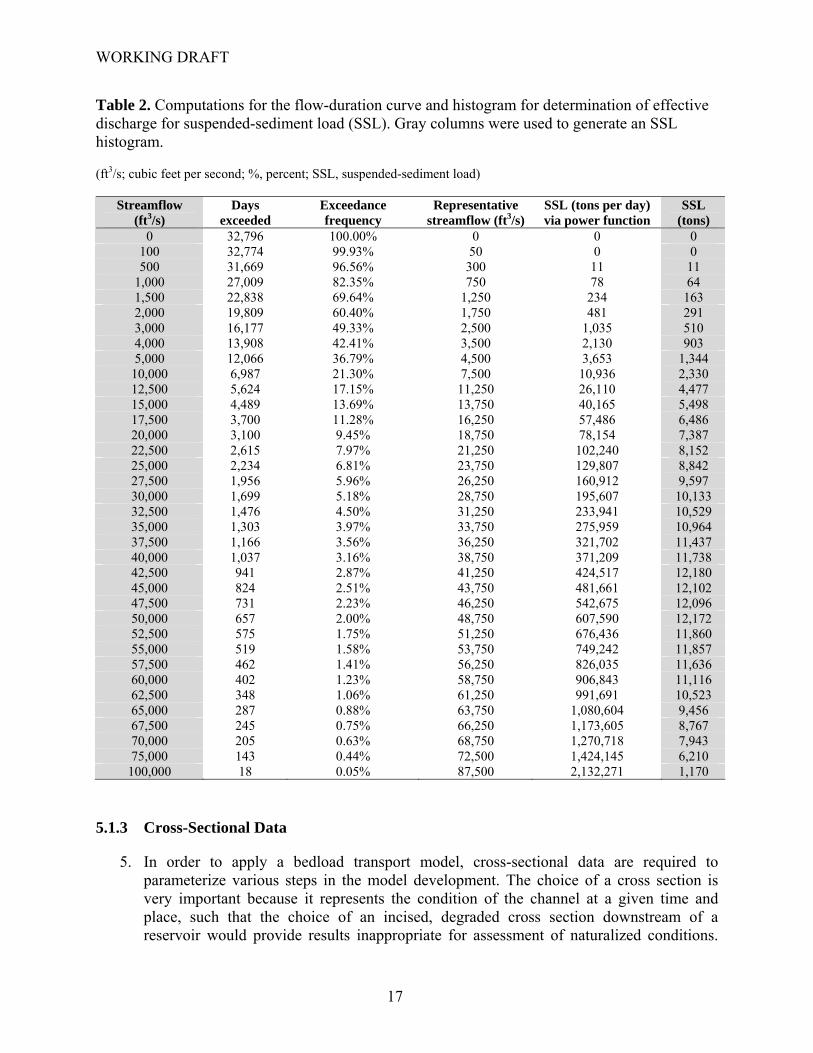
2. Suspended-sediment-load (SSL) data (period of record: February 1966 to September 1995) (tons/day) were downloaded by selecting the water quality / sediment measurements from USGS NWIS, and were exported to a spreadsheet. Records were sorted by the parameter code, and only data for suspended-sediment load were retained (USGS parameter code 80155). For days with multiple measurements of SSL, the mean value was used for that day. SSL (in log-10 space) for each day was plotted against its corresponding daily mean streamflow (in log-10 space), and a power function was fit to the data (Figure 9). The power function fitted to predict SSL from streamflow (Q) (ft3/s) is:

• SSL = (0.0000527)Q2.1463, where SSL is suspended-sediment load (tons/day) and

Q is discharge (ft3/s).

Figure 9. Suspended-sediment-load and streamflow rating curve for 08114000 Brazos River at Richmond, Texas. Scatter about the power trendline is attributed to sediment availability and hysteretic behavior of suspended-sediment concentrations over time.

3. A representative streamflow for each discharge class interval was computed as the mean discharge between two classes. The representative discharge was used in the power function determined in step #2 to compute SSL in tons/day for each discharge class. The result was multiplied by the discharge exceedance frequency to obtain the load

15

WORKING DRAFT

transported by each discharge class. Finally, the load values were plotted as a histogram for each class, using the discharge value originally used in the flow-duration curve (Figure 10). Results of the entire analysis are also presented in Table 2. It takes some iterations of this step to ensure that discharge class intervals are appropriate to accurately determine the effective discharge.

4. The effective discharge is determined by evaluating the modal class of the histogram. In this case, four discharge classes exhibited the highest suspended-sediment loads, and the mean discharge representing their bounds was selected and approximates 46,000 ft3/s, which is the effective discharge for suspended-sediment transport. Thus, for the period February 1966 to September 1995, the Brazos River at Richmond transported the cumulative majority of suspended sediment at about 46,000 ft3/s. However, this does not include bedload transport. According to the National Weather Service (NWS) West Gulf River Forecast Center (http://www.srh.noaa.gov/wgrfc/), flood stage occurs at a USGS stage of 48 feet, or 81,800 ft3/s based on the current expanded stage-discharge rating table. Therefore, effective discharge of SSL is substantially less than flood stage.

Figure 10. Suspended-sediment load (SSL) histogram showing effective discharge for SSL at 08114000 Brazos River at Richmond, Texas, approximately is 46,000 ft3/s.

16

WORKING DRAFT

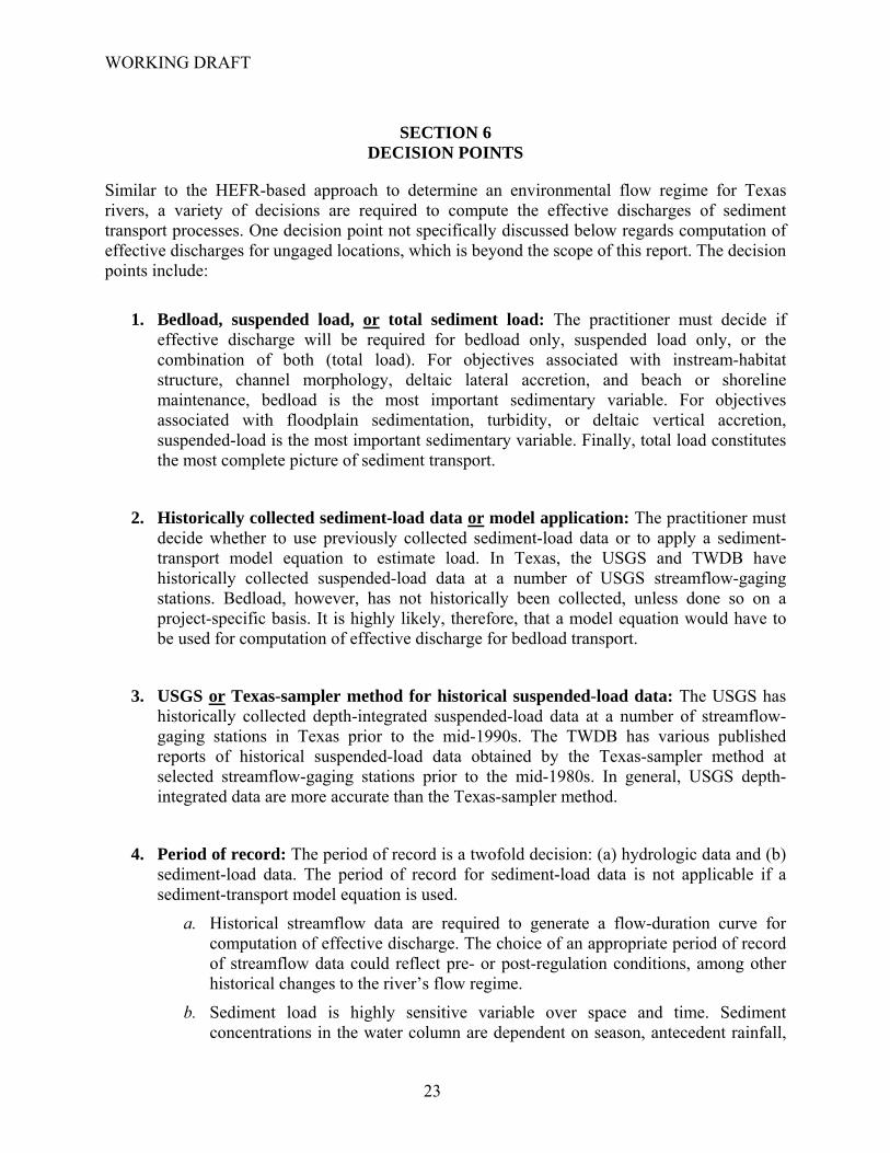
Table 2. Computations for the flow-duration curve and histogram for determination of effective discharge for suspended-sediment load (SSL). Gray columns were used to generate an SSL histogram. (ft3/s; cubic feet per second; %, percent; SSL, suspended-sediment load)

Streamflow (ft3/s)

Days exceeded

Exceedance frequency

Representative streamflow (ft3/s)

SSL (tons per day) via power function

SSL (tons)

0 32,796 100.00% 0 0 0 100 32,774 99.93% 50 0 0 500 31,669 96.56% 300 11 11

1,000 27,009 82.35% 750 78 64 1,500 22,838 69.64% 1,250 234 163 2,000 19,809 60.40% 1,750 481 291 3,000 16,177 49.33% 2,500 1,035 510 4,000 13,908 42.41% 3,500 2,130 903 5,000 12,066 36.79% 4,500 3,653 1,344

10,000 6,987 21.30% 7,500 10,936 2,330 12,500 5,624 17.15% 11,250 26,110 4,477 15,000 4,489 13.69% 13,750 40,165 5,498 17,500 3,700 11.28% 16,250 57,486 6,486 20,000 3,100 9.45% 18,750 78,154 7,387 22,500 2,615 7.97% 21,250 102,240 8,152 25,000 2,234 6.81% 23,750 129,807 8,842 27,500 1,956 5.96% 26,250 160,912 9,597 30,000 1,699 5.18% 28,750 195,607 10,133 32,500 1,476 4.50% 31,250 233,941 10,529 35,000 1,303 3.97% 33,750 275,959 10,964 37,500 1,166 3.56% 36,250 321,702 11,437 40,000 1,037 3.16% 38,750 371,209 11,738 42,500 941 2.87% 41,250 424,517 12,180 45,000 824 2.51% 43,750 481,661 12,102 47,500 731 2.23% 46,250 542,675 12,096 50,000 657 2.00% 48,750 607,590 12,172 52,500 575 1.75% 51,250 676,436 11,860 55,000 519 1.58% 53,750 749,242 11,857 57,500 462 1.41% 56,250 826,035 11,636 60,000 402 1.23% 58,750 906,843 11,116 62,500 348 1.06% 61,250 991,691 10,523 65,000 287 0.88% 63,750 1,080,604 9,456 67,500 245 0.75% 66,250 1,173,605 8,767 70,000 205 0.63% 68,750 1,270,718 7,943 75,000 143 0.44% 72,500 1,424,145 6,210

100,000 18 0.05% 87,500 2,132,271 1,170

5.1.3 Cross-Sectional Data

5. In order to apply a bedload transport model, cross-sectional data are required to parameterize various steps in the model development. The choice of a cross section is very important because it represents the condition of the channel at a given time and place, such that the choice of an incised, degraded cross section downstream of a reservoir would provide results inappropriate for assessment of naturalized conditions.

17

WORKING DRAFT

For this exercise, hard-copy USGS streamflow measurement notes for two measurements in February 1998 (moderate flow) and November 2004 (high flow) were used to construct a cross-section on the upstream side of the bridge at Richmond. The moderate flow in 1998 was used to construct the channel bed and base of the bank, and the 2004 flow was used to vertically extend the banks to a maximum stage of 33.8 feet. Based on the observed bank angle, banks were artificially extended to the NWS flood stage of 48 feet (Figure 11) The reason for using a composite of two flows was to avoid excessive bed scour during the high flow but, nonetheless, capture as much of the bank morphology as possible.

Figure 11. Cross section of 08114000 Brazos River at Richmond, Texas, based on USGS streamflow measurements in February 1998 and November 2004, and extended to NWS flood stage of 48 feet. The moderate flow of 1998 was used to construct geometry up to about 18 feet and the high flow of 2004 further extended geometry to about 34 feet.

6. The cross section was imported into WinXSPRO, a free software package available online from the U.S. Department of Agriculture Forest Service (2009). Care should be taken to correctly associate WinXSPRO results with the appropriate USGS stage because the software automatically sets the lowest point in the section to “0”. Hydraulic values, including hydraulic radius and mean velocity, for 0.25-ft stage increments were computed using the following hydraulic data for the Brazos River at Richmond, Texas, from the National Cooperative Highway Research Program (2004) CD set:

Dimensionless channel slope: 0.00012 Manning’s n: 0.03

18

WORKING DRAFT

5.1.4 Bagnold’s (1977) Bedload Model

7. For all discharge class intervals used to compute suspended-sediment load above, a series of computations were made to estimate bedload transport (Table 3). English units were used. First, mean velocity (U) (ft/s) and hydraulic radius (R) (ft) for each discharge were entered from the WinXSPRO results. Stream power per unit area (ω) (lb/s3) for each discharge class interval was computed from the following equation:

• ω = ρgdSU, where ρ is the mass density of water (62.28 lb/ft3), g is acceleration

due to gravity (32.17 ft/s2), d is mean flow depth (ft) which is considered analogous to R, S is dimensionless channel slope (0.00012), and U is mean velocity (ft/s).

Using the median particle size (D50) (ft) of bed-material for the Brazos River at Richmond from the National Cooperative Highway Research Program (2004) CD set (see below), the critical shear stress (τc) (lb/ft2) for entrainment was computed from the following equation:

• τc = τ*(ρs-ρ)D50, where τ*is the dimensionless Shields parameter (0.03 for sand-bed channels), ρs is the mass density of sediment (164.98 lb/ft3 for quartz), and D50 is the median particle size (0.00075 ft).

Average Bed Material D16, D50, D84 (in) (or the diameter at which 16, 50, and 84 percent of the sediment is finer than): 0.006, 0.009, 0.013

Next, the mean flow depth (ft) required to entrain the median particle size (D50) (ft) was

computed from the following equation:

• d = τc/( ρS)

From this value, Manning’s equation was used to compute the critical flow velocity (Uc) (ft/s) required to entrain the median particle size (D50) (ft):

• Uc = (1.49d2/3S1/2)/n, where n is Manning’s coefficient (0.03).

Next, the critical stream power (ωc) (lb/s3) required to entrain the median particle size (D50) (ft) was computed from the following equation:

• ωc = Ucτc

The Bagnold (1977) formula to estimate the bedload transport rate (Ib) (lb/ft/s) for each discharge class interval was computed from the following equation:

• Ib = (ω- ωc)3/2(d/D50)-2/3

19

WORKING DRAFT

Finally, the bedload transport rate (Ib) (lb/ft/s) was multiplied by the wetted perimeter (from WinXSPRO) for each discharge class interval to estimate a channel-wide bedload transport rate (lb/s), and the value was converted to tons/year.

Table 3. Computations for bedload transport using the Bagnold (1977) model and effective discharge for bedload. Critical stream power (ωc) was computed to be 0.00057 lb/s3 for this example. Gray columns were used to generate a bedload histogram. (ft3/s; cubic feet per second; %, percent; ft, feet; ft/s, feet per second; ω, stream power per unit bed area; lb/s3, pounds per cubic second; lb/ft/s, pounds per foot per second; yr, year)

Streamflow (ft3/s) Exceedance frequency

Stage (ft)

Mean velocity

(ft/s)

Mean depth

(ft)

Stream power (ω)

(lb/s3)

Bedload transport (lb/ft/s)

Bedload transport (tons/yr)

Bedload (tons)

100 99.93% 7.8 2.1 7.6 3.837 0.01605 62,039 61,998 500 96.56% 8.87 2.3 8.4 4.645 0.02000 79,191 76,470

1,000 82.35% 9.75 2.4 9.1 5.251 0.02278 92,393 76,090 1,500 69.64% 10.45 2.5 9.7 5.830 0.02555 105,209 73,264 2,000 60.40% 11.06 2.5 10.1 6.071 0.02642 110,481 66,731 3,000 49.33% 12.11 2.7 10.9 7.076 0.03160 135,127 66,653 4,000 42.41% 13.02 2.8 11.6 7.809 0.03515 153,075 64,916 5,000 36.79% 13.89 2.9 12.2 8.506 0.03864 171,324 63,032

10,000 21.30% 17.66 3.3 14.9 11.822 0.05541 264,034 56,251 12,500 17.15% 19.24 3.5 16.2 13.632 0.06489 315,365 54,080 15,000 13.69% 20.78 3.7 17.5 15.568 0.07522 370,302 50,686 17,500 11.28% 22.26 3.8 18.7 17.085 0.08274 412,541 46,542 20,000 9.45% 23.68 4.0 19.9 19.138 0.09411 473,693 44,775 22,500 7.97% 25.01 4.1 20.9 20.602 0.10173 518,490 41,342 25,000 6.81% 26.31 4.2 21.8 22.013 0.10925 565,418 38,515 27,500 5.96% 27.56 4.4 22.7 24.014 0.12116 636,631 37,970 30,000 5.18% 28.76 4.5 23.5 25.425 0.12899 685,881 35,532 32,500 4.50% 29.94 4.6 24.4 26.985 0.13755 737,935 33,211 35,000 3.97% 31.08 4.7 25.2 28.476 0.14593 796,713 31,654 37,500 3.56% 32.2 4.8 25.9 29.890 0.15409 850,992 30,255 40,000 3.16% 33.28 4.9 26.6 31.337 0.16250 907,706 28,701 42,500 2.87% 34.35 4.9 27.4 32.280 0.16657 940,913 26,997 45,000 2.51% 35.38 5.0 28.0 33.660 0.17482 998,564 25,089 47,500 2.23% 36.4 5.1 28.7 35.191 0.18383 1,061,660 23,664 50,000 2.00% 37.42 5.2 29.3 36.631 0.19256 1,118,126 22,399 52,500 1.75% 38.4 5.2 30.0 37.506 0.19638 1,155,837 20,265 55,000 1.58% 39.36 5.3 30.6 38.992 0.20544 1,222,095 19,340 57,500 1.41% 40.28 5.4 31.2 40.507 0.21473 1,287,515 18,137 60,000 1.23% 41.12 5.4 31.7 41.156 0.21759 1,318,420 16,161 62,500 1.06% 41.95 5.5 32.2 42.579 0.22660 1,383,729 14,683 65,000 0.88% 42.78 5.6 32.7 44.027 0.23582 1,451,174 12,699 67,500 0.75% 43.58 5.6 33.2 44.700 0.23882 1,480,947 11,063 70,000 0.63% 44.38 5.7 33.7 46.183 0.24832 1,551,610 9,699

8. A bedload histogram was plotted in the exact same manner as the suspended-load exercise (Figure 12), multiplying the final bedload (tons/year) by the exceedance frequency of the discharge for which it was modeled. The results show that effective

20

WORKING DRAFT

discharge for cumulative bedload transport occurs at relatively low flows. This, however, is an inaccurate assessment of bedload transport in reality. The Bagnold (1977) model is dependent on excess stream power, which is generated to a large measure by depth and velocity. The flaw in this example occurred because the stage for very low flows according to the USGS, say 100 ft3/s, filled up the cross section to a mean depth of 7.6 feet at a mean velocity of 2.1 ft/s according to hydraulic computations modeled in WinXSPRO. These modeled hydraulic conditions are more than adequate at transporting sand-sized bedload, and their almost constant occurrence over time ensured low flows outpaced moderate to high flows with respect to cumulative transport. In reality, the hydraulic conditions at 100 ft3/s at this cross section are sluggish and pond-like, not capable of transporting sand-sized bedload. Furthermore, it is very unusual for bedload to exceed suspended-load transport, thereby providing additional evidence for the problematic data used to compute bedload. This example underscores the importance of selecting an appropriate cross section to model bedload transport using any given equation. For appropriate cross sections with adequate data, however, the Bagnold (1977) equation has worked well for other investigations.

Figure 12. Bedload histogram showing an inaccurately low estimate of effective discharge for bedload at 08114000 Brazos River at Richmond, Texas.

9. Finally, the practitioner can combine suspended load (tons) and bedload (tons) for a given flow to evaluate the effective discharge for total sediment load.

21

WORKING DRAFT

22

5.2 ADVOCACY OF THE SAM HYDRAULC DESIGN MODEL

The SAM hydraulic design model efficiently computes the exercises shown above when parameterized with sufficient data. Furthermore, SAM can recommend appropriate sediment transport formulae for the given input, such as channel slope and bed-material particle size. The use of the SAM hydraulic design model is a tool that can be used to establish effective discharge at gaging stations, but should be done by an expert in the field of fluvial geomorphology or sediment transport dynamics. As discussed above, effective discharge should be applied with caution for rivers that do not exhibit steady-state equilibrium. The SAM model requires cross-sectional geometry data for the location of interest. For rivers that are degraded, such as those that have incised immediately below reservoirs, cross-sectional channel geometry probably is not representative of any natural condition. As a hypothetical example, cross-sectional area of a river channel immediately downstream of a reservoir is greatly enlarged as a result of channel incision and bank retreat, and SAM computes a sediment load much greater for the enlarged channel than would be expected naturally. Because the sediment transport models embedded within SAM are based on equilibrium-based theoretical constructs, however, the output of the model provides the analyst with a reference condition of sediment transport. As such, SAM output can be used in conjunction with field measurements of suspended load and bedload to determine if the river is over- or under-achieving with respect to sediment transport. Regardless of the analysis employed, values of effective discharge should be considered with respect to desired conditions of particular river systems. For some rivers, it might be desirable to transport less sediment load than that computed by an effective discharge analysis. As a hypothetical example, a river reach 25 miles downstream of a reservoir receives much less sediment than it did during pre-impoundment conditions. In order to prevent channel incision and associated bank failure over time, it would be desirable for sediment transport to underperform that predicted by a SAM analysis of steady-state conditions. Another serious concern related to the practicality of effective discharge for environmental flow programs is the stasis of its approach. If an existing flow regime is modified to satisfy a prescription, then it is likely that the magnitude and frequency of the effective discharge changes as well. Iterations of effective discharge overlays and subsequent modification of the flow regime becomes impractical at some level.

WORKING DRAFT

SECTION 6 DECISION POINTS

Similar to the HEFR-based approach to determine an environmental flow regime for Texas rivers, a variety of decisions are required to compute the effective discharges of sediment transport processes. One decision point not specifically discussed below regards computation of effective discharges for ungaged locations, which is beyond the scope of this report. The decision points include:

1. Bedload, suspended load, or total sediment load: The practitioner must decide if effective discharge will be required for bedload only, suspended load only, or the combination of both (total load). For objectives associated with instream-habitat structure, channel morphology, deltaic lateral accretion, and beach or shoreline maintenance, bedload is the most important sedimentary variable. For objectives associated with floodplain sedimentation, turbidity, or deltaic vertical accretion, suspended-load is the most important sedimentary variable. Finally, total load constitutes the most complete picture of sediment transport.

2. Historically collected sediment-load data or model application: The practitioner must

decide whether to use previously collected sediment-load data or to apply a sediment-transport model equation to estimate load. In Texas, the USGS and TWDB have historically collected suspended-load data at a number of USGS streamflow-gaging stations. Bedload, however, has not historically been collected, unless done so on a project-specific basis. It is highly likely, therefore, that a model equation would have to be used for computation of effective discharge for bedload transport.

3. USGS or Texas-sampler method for historical suspended-load data: The USGS has

historically collected depth-integrated suspended-load data at a number of streamflow-gaging stations in Texas prior to the mid-1990s. The TWDB has various published reports of historical suspended-load data obtained by the Texas-sampler method at selected streamflow-gaging stations prior to the mid-1980s. In general, USGS depth-integrated data are more accurate than the Texas-sampler method.

4. Period of record: The period of record is a twofold decision: (a) hydrologic data and (b)

sediment-load data. The period of record for sediment-load data is not applicable if a sediment-transport model equation is used.

a. Historical streamflow data are required to generate a flow-duration curve for computation of effective discharge. The choice of an appropriate period of record of streamflow data could reflect pre- or post-regulation conditions, among other historical changes to the river’s flow regime.

b. Sediment load is highly sensitive variable over space and time. Sediment concentrations in the water column are dependent on season, antecedent rainfall,

23

WORKING DRAFT

land-use, characteristics of the storm hydrograph, and upstream impoundments, among other variables. The period of record for measured sediment-load data could reflect pre- or post-regulation conditions, among other historical changes to the river’s sediment-transport regime.

5. Flow-duration class intervals: A flow-duration curve requires the practitioner to

establish “class intervals” which are related to exceedance frequency of that interval’s representative flow. Although various published sources offer guidance on establishing class intervals, the choice is relegated to the practitioner. Accuracy of effective discharge increases if class intervals are shorter and more numerous (e.g., class intervals of 1,000 ft3/s are more accurate than 5,000 ft3/s).

6. Sediment-transport model: This decision is only required if the practitioner does not

have or chooses not to use measured sediment-load data to determine effective discharge. A variety of model equations exist that estimate bedload transport rates for various flow conditions, and are based on measured or estimated parameters. Bedload equations commonly are suited to particular conditions, such as a low-gradient sand-bed channel, for example. Other model equations exist that estimate suspended-load transport rates using either measured or estimated parameters. The choice of an appropriate model equation is relegated to the practitioner, possibly with guidance from the SAM hydraulic design model.

7. Channel cross-section dimensions: This decision is only required if using a model

equation to estimate sediment load. Cross-sectional data are needed to compute channel hydraulics (e.g., width, mean depth, mean velocity) based on a given slope and flow-resistance coefficient. Further, most model equations render sediment-load estimates for a given channel length, and require a wetted perimeter for extrapolation to channel-wide transport rates. As shown from the Brazos River at Richmond, Texas, example above, an unrepresentative cross section can lead to erroneous results. Cross-sectional dimensions could be chosen to represent pre- or post-regulation conditions, pre- or post-disturbance conditions, straight-reach or meander-bend conditions, among other complex arrangements of channel shape over space and time.

8. Model parameters: This decision is only required if using a model equation to estimate

sediment load. Various parameters, including channel slope, particle size, mean depth, and water temperature, among others, are needed to parameterize sediment-transport model equations and compute selected hydraulics at a channel cross section. Various published and unpublished sources exist that provide this information. For certain applications, the practitioner could elect to estimate required parameters.

9. Extrapolation of effective discharge to a channel reach: As outlined above,

computation of effective discharge is restricted to one channel cross section. Given this

24

WORKING DRAFT

restriction, environmental flow objectives associated with sediment transport are valid for one station. If desired, extrapolation to a channel reach should consider variability in sediment sources and sinks upstream and downstream of the station, including tributary inputs, distributary outputs, active bank erosion, channel incision or aggradation, overbank deposition, among other complex watershed and channel characteristics and processes.

25

WORKING DRAFT

SECTION 7 CONCLUSIONS

An analysis of effective discharge of suspended-sediment load (SSL), bedload, and/or total load at streamflow-gaging stations could be used to modify HEFR-based flow prescriptions for establishing environmental flows. For the majority of locations, the high-pulse flow or overbank-flow categories are associated with the cumulative majority of sediment transport over time. Computations for suspended load should utilize historical measurements, if available, and bedload likely requires application of a model equation. Sediment transport, although relatively straightforward in its association with discharge, does not encompass the breadth of fluvial geomorphic processes. Furthermore, concepts of steady-state equilibrium challenge assumptions that a constant discharge value is responsible for the cumulative majority of sediment transport over time. Finally, practitioners utilizing effective discharge for rivers in Texas should be cognizant of the contemporary sediment-transport regime and historical channel adjustments at each location considered. Assignment of an effective discharge to altered or regulated rivers is problematic and implementation efforts could be harmful if a holistic perspective (e.g., sediment trapped behind reservoirs, non-representative cross section to estimate bedload transport, etc.) is not considered.

26

WORKING DRAFT

SECTION 8 REFERENCES

Ackers, P., and White, W.R., 1973, Sediment transport—New approach and analysis: ASCE Journal of the Hydraulics Division, v. 99(HY11), p. 2,041–2,060.

Adey, E.A., and Cook, H.M., 1964, Suspended-sediment load of Texas streams—Compilation report—October 1959–September 1961: Texas Water Commission Bulletin 6410, 50 p.

Andrews, E.D., 1980, Effective and bankfull discharges of streams in the Yampa River Basin, Colorado and Wyoming: Journal of Hydrology, v. 46, p. 311–330.

Andrews, E.D., and Nankervis, J.M.,1995, Effective discharge and the design of channel maintenance flows for gravel-bed rivers, in Costa, J.E., Miller, A.J., Potter, K.W., and Wilcock, P.R., eds., Natural and anthropogenic influences in fluvial geomorphology: Washington, D.C., American Geophysical Union, p. 151–164.

Bagnold, R.A., 1977, Bed load transport by natural rivers: Water Resources Research, v. 13, p. 303–312.

Bagnold, R.A., 1980, An empirical correlation of bedload transport rates in flumes and natural rivers: Proceedings of the Royal Society of London, v. 372A, p. 453–473.

Biedenharn, D.S., Copeland, R.R., Thorne, C.R., Soar, P.J., Hey, R.D., and Watson, C.C., 2000, Effective discharge calculation—A practical guide: United States Army Corps of Engineers ERDC/CHL TR-00-15, 63 p.

Biedenharn, D.S., Little, C.D., and Thorne, C.R., 1999, Magnitude-frequency analysis of sediment transport in the Lower Mississippi River: Vicksburg, Miss., U.S. Army Corps of Engineers, Miscellaneous Paper CHL–99–2.

Bourke, M.C., and Pickup, G., 1999, Fluvial form variability in arid central Australia, in Miller, A.J., and Gupta, A., eds., Varieties of fluvial form: Chichester, UK, Wiley, p. 249–271.

Brierley, G.J., and Fryirs, K.A., 2005, Geomorphology and river management—Applications of the River Styles Framework: Malden, Mass., Blackwell, 398 p.

Cook, H.M., 1967, Suspended-sediment load of Texas streams—Compilation report—October 1961–September 1963: Texas Water Development Board Report 45, 62 p.

Cook, H.M., 1970, Suspended-sediment load of Texas streams—Compilation report—October 1963–September 1965: Texas Water Development Board Report 106, 63 p.

Dougherty, J.P., 1979, Suspended-sediment load of Texas streams—Compilation report—October 1971–September 1975: Texas Water Development Board Report 233, 83 p.

27

WORKING DRAFT

Edwards, T.K., and Glysson, G.D., 1999, Field methods for measurement of fluvial sediment: U.S. Geological Survey Techniques of Water-Resources Investigations, Book 3, Chapter C2, 89 p.

Einstein, H.A., 1950, The bedload function for sediment transportation in open channel flows: U.S. Department of Agriculture Technical Bulletin 1026.

Gomez, B., 2006, The potential rate of bed-load transport: Proceedings of the National Academy of Sciences, v. 103, p. 17,170–17,173.

Gomez, B., and Church, M., 1989, An assessment of bed load sediment transport formulae for gravel bed rivers: Water Resources Research, v. 25, p. 1,161–1,186.

Gomez, B., and Phillips, J.D., 1999, Deterministic uncertainty in bed load transport: Journal of Hydraulic Engineering, v. 125, p. 305–308.

Gupta, A., 1988, Large floods as geomorphic events in the humid tropics, in Baker, V.R., Kochel, R.C., and Patton, P.C., eds., Flood geomorphology: Chichester, UK, Wiley, p. 301–315.

Hudson, P.F., 2003, Event sequence and sediment exhaustion in the lower Pánuco basin, Mexico: Catena, v. 52, p. 57–76.

Hudson, P.F., and Mossa, J., 1997, Suspended sediment transport effectiveness of three, large impounded rivers, U.S. Gulf Coastal Plain: Environmental Geology, v. 32, p. 263–273.

Knighton, D., 1998, Fluvial forms and processes—A new perspective: London, Arnold, 383 p.

Kondolf, G.M., 1994, Geomorphic and environmental effects of instream gravel mining: Landscape and Urban Planning, v. 28, p. 225–243.

McKnight, T.L., and Hess, D., 2000, Physical geography—A landscape appreciation, 6th ed.: Upper Saddle River, N.J., Prentice Hall, 604 p.

Meyer-Peter, R., and Müller, R., 1948, Formulas for bedload transport, in Proceedings 2nd Meeting International Association of Hydraulic Research: Stockholm, p. 39–64.

Mirabal, J., 1974, Suspended-sediment load of Texas streams—Compilation report—October 1965–September 1971: Texas Water Development Board Report 184, 121 p.

National Cooperative Highway Research Program, 2004, Archived river meander bend database: Washington, D.C., Transportation Research Board of the National Academies, 4 CD-set.

National Research Council of the National Academies, 2005, The science of instream flows—A review of the Texas Instream Flow Program: Washington, The National Academies Press, 149 p.

28

WORKING DRAFT

Parker, G., Klingeman, P.C., and McLean, D.G., 1982, Bedload and size distribution in paved gravel-bed streams: ASCE Journal of the Hydraulics Division, v. 108(HY4), p. 544–571.

Quincy, R.M., 1988, Suspended sediment load of Texas streams—Compilation report, October 1975–September 1982: Texas Water Development Board Report 306, 153 p.

Ritter, D.F., Kochel, R.C., and Miller, J.R., 2002, Process geomorphology, 4th ed.: New York, McGraw-Hill, 560 p.

Robert, A., 2003, River processes—An introduction to fluvial dynamics: London, Arnold, 214 p.

Schumm, S.A., 1977, The fluvial system: New York, John Wiley, 338 p.

Senate Bill 3 Science Advisory Committee for Environmental Flows, 2009, DRAFT—Use of hydrologic data in the development of instream flow recommendations for the environmental flows allocation process and the hydrology-based environmental flow regime (HEFR) methodology: SAC-2009-01, 46 p.

Stout, I.M., Bentz, L.C., and Ingram, H.W., 1961, Silt load of Texas streams—A compilation report—June 1889–September 1959: Texas Board of Water Engineers Bulletin 6108, 237 p.

Texas Commission on Environmental Quality, Texas Parks and Wildlife Department, and Texas Water Development Board, 2008, Texas Instream Flow Studies—Technical Overview: Texas Water Development Board Report 369, 137 p.

Torizzo, M., and Pitlick, J., 2004, Magnitude-frequency of bed load transport in mountain streams in Colorado: Journal of Hydrology, v. 290, p. 137–151.

U.S. Department of Agriculture Forest Service, 2009, WinXSPRO version 3.0: at http://www.stream.fs.fed.us/publications/winxspro.html

U.S. Geological Survey, 2009, National Water Information System (NWIS), accessed January 2009, at http://waterdata.usgs.gov/nwis

Welborn, C.T., 1967, Comparative results of sediment transport sampling with the Texas sampler and the depth-integrated samplers and specific weight of fluvial sediment deposits in Texas: Texas Water Development Board Report 36.

Wolman, M.G., and Miller, J.P., 1960, Magnitude and frequency of forces in geomorphic processes: Journal of Geology, v. 68, p. 54–74.

29

WORKING DRAFT

30

SECTION 9 GLOSSARY

Bedload: a measure of the transport of fluvial sediment along or near the channel bed by traction or saltation mechanisms; either sand, gravel, or larger size; expressed as mass over time

Bed-material load: a measure of the transport of fluvial sediment as bedload or sand grains in suspension during turbulent flows; only comprised of particles derived from the channel bed; does not include silt or clay particles; expressed as mass over time

Effective discharge: the flow rate responsible for the majority of cumulative sediment transport over time; usually equated to a relatively frequent, moderate flow event; commonly accepted as bankfull discharge; association with bankfull discharge is less apparent for fluvial systems with a highly-variable flow regime

Saltation: a mechanism of bedload transport where particles skip along the channel bed

Sediment budget: a technique that accounts for sources (additions) and sinks (subtractions) of fluvial sediment in a defined system (e.g., watershed); accounts for sources from hillslopes, channel banks, tributaries, among others; accounts for removals from impoundments, floodplain storage, distributaries, among others

Steady-state equilibrium: concept that a river channel adjusts over graded time (decades to hundreds of years) to efficiently convey the amount of discharge and sediment load by maintaining a particular slope, pattern, and shape; suggests that the fluvial system will gradually recover from the effects of a disturbance to the system (e.g., 100-year flood); a fundamental, but controversial, fluvial geomorphic concept

Stream power: the product of average shear stress and average velocity; commonly used to predict sediment transport; expressed in SI units as watts/square meter

Suspended-sediment load: a measure of the transport of fluvial sediment continuously entrained in the water column; mostly clay and silt, with varying amounts of sand derived from the channel bed during turbulent flows; expressed as mass over time

Suspended-sediment concentration: the concentration of suspended sediment in the water column; computed as the ratio of suspended-sediment load to the streamflow; expressed as milligrams per liter

Traction: a mechanism of bedload transport where particles roll or slide along the channel bed

Wash load: a measure of the transport of fluvial sediment and other material continuously entrained in the water column (e.g., clay, silt, and organic matter); does not include the sand-sized fraction; expressed as mass over time

WORKING DRAFT

SECTION 10 CONTRIBUTORS

Contributor and Contact Information Franklin Heitmuller, ftheitmu@usgs.gov

Commentor and Contact Information TWDB: Greg Malstaff, greg.malstaff@twdb.state.tx.us

31