Montréal Juin 2003

© 2003 Benoît Bourbeau, Teodor Grabriel Crainic, Michel Gendreau, Jacques Robert. Tous droits réservés. All rights reserved. Reproduction partielle permise avec citation du document source, incluant la notice ©. Short sections may be quoted without explicit permission, if full credit, including © notice, is given to the source.

Série Scientifique Scientific Series

2003s-36

Design for Optimized Multi-Lateral Multi-Commodity Markets

Benoît Bourbeau, Teodor Grabriel Crainic,

Michel Gendreau, Jacques Robert

CIRANO

Le CIRANO est un organisme sans but lucratif constitué en vertu de la Loi des compagnies du Québec. Le financement de son infrastructure et de ses activités de recherche provient des cotisations de ses organisations-membres, d’une subvention d’infrastructure du ministère de la Recherche, de la Science et de la Technologie, de même que des subventions et mandats obtenus par ses équipes de recherche.

CIRANO is a private non-profit organization incorporated under the Québec Companies Act. Its infrastructure and research activities are funded through fees paid by member organizations, an infrastructure grant from the Ministère de la Recherche, de la Science et de la Technologie, and grants and research mandates obtained by its research teams.

Les organisations-partenaires / The Partner Organizations PARTENAIRE MAJEUR . Ministère du développement économique et régional [MDER] PARTENAIRES . Alcan inc. . Axa Canada . Banque du Canada . Banque Laurentienne du Canada . Banque Nationale du Canada . Banque Royale du Canada . Bell Canada . Bombardier . Bourse de Montréal . Développement des ressources humaines Canada [DRHC] . Fédération des caisses Desjardins du Québec . Gaz Métropolitain . Hydro-Québec . Industrie Canada . Ministère des Finances [MF] . Pratt & Whitney Canada Inc. . Raymond Chabot Grant Thornton . Ville de Montréal . École Polytechnique de Montréal . HEC Montréal . Université Concordia . Université de Montréal . Université du Québec à Montréal . Université Laval . Université McGill ASSOCIÉ AU : . Institut de Finance Mathématique de Montréal (IFM2) . Laboratoires universitaires Bell Canada . Réseau de calcul et de modélisation mathématique [RCM2] . Réseau de centres d’excellence MITACS (Les mathématiques des technologies de l’information et des systèmes complexes)

ISSN 1198-8177

Les cahiers de la série scientifique (CS) visent à rendre accessibles des résultats de recherche effectuée au CIRANO afin de susciter échanges et commentaires. Ces cahiers sont écrits dans le style des publications scientifiques. Les idées et les opinions émises sont sous l’unique responsabilité des auteurs et ne représentent pas nécessairement les positions du CIRANO ou de ses partenaires. This paper presents research carried out at CIRANO and aims at encouraging discussion and comment. The observations and viewpoints expressed are the sole responsibility of the authors. They do not necessarily represent positions of CIRANO or its partners.

Design for Optimized Multi-Lateral Multi-Commodity Markets

Benoît Bourbeau*, Teodor Gabriel Crainic†, Michel Gendreau‡, Jacques Robert§

Résumé / Abstract Nous présentons un concept de marché optimisé, centralisé, multilatéral et périodique pour l’acquisition de produits qui traite explicitement les trois aspects suivants: (i) des coûts de transport importants des vendeurs vers les acheteurs; (ii) des produits non homogènes en valeur et qualité; des complémentarités entre les divers produits qui doivent donc être négociés simultanément. Le modèle permet aux vendeurs d’offrir leurs produits groupés en lots et aux acheteurs de quantifier explicitement leur évaluation des lots mis sur le marché par chaque vendeur. Le modèle ne suppose pas que les produits doivent être expédiés par un centre avant d’être livrés. Nous proposons également un mécanisme de tâtonnement à rondes multiples qui approxime le comportement du marché direct optimisé et qui permet de mettre ce dernier en oeuvre. Le processus de tâtonnement permet aux vendeurs et aux acheteurs de modifier leurs mises initiales, incluant les contraintes technologiques. Les concepts proposés sont particulièrement adaptés aux industries reliées aux matières premières. Nous présentons les modèles et algorithmes requis à la mise en oeuvre du marché multi-latéral optimisé, nous décrivons le fonctionnement du processus de tâtonnement, et nous discutons les applications et perspectives reliées à ces mécanismes de marché.

Mots clés : Design de marché, marché multi-latéraux optimisés, processus de tâtonnement.

In this paper, we propose a design for an an economically efficient, optimized, centralized, multi-lateral, periodic commodity market that addresses explicitly three issues: (i) substantial transportation costs between sellers and buyers; (ii) non homogeneous, in quality and nature, commodities; (iii) complementary commodities that have to be traded simultaneously. The model allows sellers to offer their commodities in lots and buyers to explicitly quantify the differences in quality of the goods produced by each individual seller. The model does not presume that products must be shipped through a market hub. We also propose a multi-round

* CIRANO, email: bourbeab@cirano.qc.ca. † Département management et technologie, Université du Québec à Montréal and CIRANO and Centre de recherche sur les transports, Université de Montréal/École Polytechnique/HEC Montréal, email: theo@crt.umontreal.ca. ‡ Département d’informatique et recherche opérationnelle, Université de Montréal and CIRANO and Centre de recherche sur les transports, Université de Montréal/École Polytechnique/HEC Montréal, email: michelg@crt.umontreal.ca. § Département des Technologies de l’information, HEC Montréal and CIRANO, email: jacques.robert@hec.ca.

auction that enables the implementation of the direct optimized market and approximates the behaviour of the “ideal” direct optimized mechanism. The process allows buyers and sellers to modify their initial bids, including the technological constraints. The proposed market designs are particularly relevant for industries related to natural resources. We present the models and algorithms required to implement the optimized market mechanisms, describe the operations of the multi-round auction, and discuss applications and perspectives.

Keywords: Market design, optimized multi-lateral multi-commodity markets, multi-round auctions.

1 Introduction

Until very recently markets were not designed, they just existed. Markets emerged out ofuncoordinated private initiatives and, in most cases, there are still no explicit rules thatdetermine how equilibrium prices are discovered and set. In most markets, prices are postedby sellers or negotiated bilaterally according to informal rules. Recently, however, the designof market rules has emerged as a very important issue due to three main factors: (i) Thecreation by government agencies, private firms or industrial associations of a number ofmarkets to privatize public assets, restructure deregulated industries, or enhance inter-firmrelations; (ii) A renewed focus on strategic analysis and game theory that together with theemergence of experimental economics contributed to the establishment of market design asa serious research field in economics; (iii) And, most importantly, the explosive developmentof electronic business, e-business tools that can embed the most complex market rules andfacilitate their deployment.

This paper examines the problem of designing optimized or smart markets. An optimizedor smart market is an advanced exchange mechanism. It is a competitive environment wherebuyers and sellers interact and is designed to solve possibly complex allocation problems.According to Miller (1996), “the distinctive characteristic of a smart market is that it canmanage complex contingencies embedded within orders in a consistent and effective manner.”A smart market would generally require an optimization device in order to clear the marketwhile taking into account the implicit or explicit constraints and contingencies submitted tothe market marker. There are typically two types of constraints: complex order requirementsas submitted by the participants and feasibility requirements as some orders may not bejointly fulfilled. A number of smart market mechanisms have been proposed for pricing theInternet (MacKie-Mason and Varian 1995; MacKie-Mason 1997) and for allocating accessesto a railway network (Brewer and Plott 1996), airport take-off and landing slots (Rassenti,Smith, and Bulfin 1982; Grether, Isaac, and Plott 1989), and pollution permits (Marron andBartels 1996), as well as for the scheduling of the Space station resources (Ledyard, Porter,and Rangel 1994), the distribution of electricity within a grid (Rothkopf, Kahn, Teisberg,Eto, and Nataf 1990), and the matching of supply and demand in financial markets (Fan,Stallaert, and Whinston 1999). A number of authors have also addressed issues related to theoptimization formulations of market clearance mechanisms, in particular in combinatorialauctions (e.g., Rothkopf, Pekec, and Harstad 1998; Sandholm 1999; De Vries and Vohra2001; Kalagnanam, Davenport, and Le 2001; DeMartini, Kwasnica, Ledyard, and Porter1999) where participants may submit “all-or-nothing” package bids.

Yet, relatively few actual implementations of smart markets have been observed up tonow. Furthermore, very limited efforts have been dedicated to the design of the whole marketmechanism (Abrache, Crainic, and Gendreau 2001). With a growing interest on the use ofcombinatorial auctions for spectrum rights, the trend seems to be changing, however, anda consensus appears to emerge that optimized markets can be profitably used in complexenvironments where global efficiency is highly desirable. Therefore, the general objective ofthis paper is to contribute to the development of the basic methodology leading to the design

1

and practical implementations of optimized markets.

A market design must specify clear negotiation rules. These include two main elements.First, one must specify an explicit mathematical representation for the market-clearing pro-cedure that identifies, given the submitted bids, the market allocation, who produces whatand sells to whom and in what quantities, and prices, who pays what to whom. Formally,under certain conditions, a market-clearing mechanism can be represented as a constrainedoptimization problem. The bids define the parameters of the constrained optimization prob-lem, while the solution of the problem yields the quantity allocation (the primal) and thecorresponding prices (usually based on dual information). Second, the market design mustspecify how negotiations will proceed.

It is well known, in effect, that participants often are unwilling or unable to discloseall the pertinent but very personal and proprietary information required for an optimizedmarket. Moreover, formal incentive mechanisms cannot be defined for many important mar-ket cases, including the multi-lateral type of market considered in this paper (Myerson andSatterthwaite 1983). Open, multi-round negotiations are therefore increasingly considered.Such multi-round auctions require significantly less a priori information and allow partic-ipants to alter their selling or buying offers in light of the market information and theirown assessment of the market. At each round, the auction makes use of the optimizationprocedure to produce a temporary set of allocations and prices. The process continues untilno one wishes to alter its bid and the bilateral exchanges then become official. In order toprevent the negotiation from lasting for ever, the rules must specify not only the stoppingrule, however, but also eligibility and activity rules whose function is to give impetus to themarket by prompting participants to be active and progressively commit themselfs.

We focus on the design of optimized multi-lateral markets for geographically dispersedheterogeneous commodities and technological constraints. Based on well-known economicprinciples, we define an economically efficient optimized multi-lateral market that addressesexplicitly four issues: (i) the non homogeneity in quality and nature of the commoditiestraded, (ii) the buyers’ qualification of the differences in quality of the goods producedby each individual seller, (iii) the existence of complementarities between commodities andthe need to negotiate these simultaneously, (iv) the presence of substantial transportationcosts between sellers and buyers. We strongly believe that when transportation costs aresignificant, they should be explicitly accounted for in the optimization of the market. Howthis can be achieved in practice is one of the main contributions of the paper. We presentthe appropriate optimization formulations and algorithms, and define an open, multi-roundauction mechanism that enables the implementation of the optimized multi-lateral marketand approximates its behaviour under “ideal” information conditions. We show how such amechanism may be operationalized and present simulation results that illustrate some of thegains that can be obtained by using smart market mechanisms. Finally, we report on someof the difficulties encountered in “selling” the proposal to industrial actors.

The paper is organized as follows. Section 2 presents the optimization formulation wepropose to model the operations of the centralized market mechanism. We introduce the

2

main concepts and notation, present the model, and derive the market equilibrium conditions.Section 3 describes the optimization algorithms used to determine the optimal allocation andprices. Section 4 is dedicated to the presentation and analysis of the multi-round auctionmechanism and the description of how negotiations are conducted. Section 5 briefly describesthe Quebec wood chip industry, which prompted the work presented in this paper, andpresents the simulation results. Double-sided markets of the type studied in this paper arehard to analyze from a formal point of view. In particular, there is no theory describinghow participants interact in such a market and classical incentive mechanisms do not apply.Therefore, Section 5 also presents a strategic analysis of the proposed market mechanismand addresses the issue of applying it, both in general and in the particular context of thewood chip market. We conclude in Section 6.

2 Allocation Mechanisms for Optimized Multi-lateral

Multi-commodity Markets

We propose a design for an optimized, centralized, multi-lateral, periodic commodity mar-ket. The market opens up periodically (once a day, once a week) and the agents in thecorresponding economic sector negotiate using the centralized and optimized market. Allpossible multi-lateral trades are thus solved simultaneously. Commodities are classified bytype or quality. Sellers may offer several commodity types separately or mixed up in lots.Buyers need to combine different grades and qualities, while technological constraints limitthe quantities of each type of commodity they may acquire. Transportation costs are sig-nificant. The objective of this type of markets is to explicitly optimize both the productionand transportation of resources in the industry.

At the core of the market lies a market-clearing mechanism: a formal procedure thatdetermines the “optimal” allocation - who sells what (how much) to whom and at what price- of goods given the participants and the market state. Participants are asked to communicateto the central market their production cost or demand functions (their willingness to pay),together with all relevant technical information: transportation costs, technical constraints,etc. The market then maximizes buyers’ surplus minus the production and transportationcosts subject to all technological constraints. The output of the allocation mechanism areprices and quantities that equilibrate supply and demand, and that are the solution (dualand primal) of an optimization (maximization) formulation. This approach applies for amarket with a simple structure as well as for more complex markets.

To fix ideas, consider first a simple market where a unique homogeneous commodityis traded between one buyer and one seller. Assume no transportation costs are involved.Assuming the buyer and seller have quasi-linear utilities in money, their preferences are givenby U(q) − S and S − C(q), respectively, where q is the quantity sold by the seller againsta payment of S. In such a market, total profit is maximized and efficiency is obtained bysolving the optimization problem maxq{U(q)− C(q)}.

3

At the optimum allocation, q∗, the marginal willingness to pay, U 0(q∗), equals the marginalproduction cost, C 0(q∗). Following the Marshallian partial equilibrium tradition, this is nodifferent from equalizing supply and demand, where the demand and supply functions cor-respond to the marginal utility and cost curves, respectively. The equilibrium price is givenby p∗ = U 0(q∗) = C 0(q∗). Transportation costs may be considered by explicitly introducingthem into the optimization problem. For a constant transportation unit cost t, one needs tosolve maxq{U(q)− C(q)− tq}. The buyer then pays p∗ = U 0(q∗) = C 0(q∗) + t per unit pur-chased, the seller receives p∗− t = C 0(q∗), and the carrier receives t per unit. This approachmay be generalized to more complex environments as described in the following subsection.

2.1 The Optimized Allocation Mechanism

The objective is to formulate a model to represent the products on sale in the market,the preferences of buyers and sellers regarding these products, the technological constraintsbuyers face, the transportation costs associated to delivering the products to the buyers. Thegoal is to maximize the buyers’ surplus, to obtain a so-called efficient market. The model isto be solved by mathematical programming techniques: the primal solution corresponds tothe optimal quantities bought, while the dual yields the optimal prices.

Let K be the set of products. The definition of a product is domain specific. Generallyspeaking, however, a product is a generic classification reference, such as a quality of ore,a wood species, a type of grain, etc. It is a commodity differentiated by type and quality.Even though the number of products in a market may be limited, products can be variouslycombined in different lots that sellers and buyers may trade. To simplify the presentation(but with no loss of generality), a lot l ∈ L is sold by one and only one seller. It is attachedto a specific location and has its own idiosyncratic quality. Since a producer may sell morethan one lot, the number of lots may exceed the number of producers. More importantly,a lot has its own composition of various products. For example, a stack of wood chips maycontains 60% of high density fiber, 35% of low density fiber, and 5% of grey pine. Beforerefinement, a stack of ore or a barrel of petroleum may contain different types of ores or oilsand, in practice, it may be sold before the different types of oils or ores are separated. Letbkl denote the proportion of product k ∈ K in lot l , where

Pk bkl = 1. A maximum quantity

of Ql is available for lot l.

Let J be the set of buyers. Buyers face technological constraints and use proprietaryrecipes. We thus assume that a buyer desires to acquire a certain mix of products (firmsdesiring more then one mix are represented as more than one buyer). On the other hand,lots may display very different product characteristics, even when the same product typesare involved. Consequently, to ensure maximum flexibility and adaptability, the marketdesign we propose allows buyers to express preferences for the lots offered for sale. Buyerpreferences are modeled as two (quality) adjustment coefficients: one multiplicative, rlj, andone additive, slj, for buyer j ∈ J and lot l ∈ L. The former may be interpreted as follows:for buyer j, one unit of lot l is equivalent to rlj units of a standard lot. If r

lj > 1 (r

lj < 1),

4

then one unit of lot l is more (less) valuable than a standard unit. On the other hand, sljmeans that for buyer j one unit of lot l is worth slj dollars more than a standard unit. LetMkj (m

kj ) denote the maximum (minimum) proportion of product k ∈ K that buyer j is

ready to accept in the mix it purchases, while Qj indicates the maximum total quantity ofall products the buyer requires. Unit transportation costs between the seller of lot l andbuyer j are denoted tlj.

Buyer and seller preferences are represented by utility and cost functions, respectively.Denote by Uj(·) the utility function of buyer j ∈ J , and by Cl(·) the cost or productionfunction of lot l ∈ L. According to classical economic theory, the utility function correspondsto the integral below the demand curve, U 0j(q), of buyer j that stands for the marginal benefitfor buyer j to acquire the qth unit. It is usually assumed that U 0j(q) is continuous, piece-wiselinear, and strictly decreasing (see Figure 1). Hence, Uj(·) is concave. Symmetrically, thecost function Cl(q) corresponds to the integral of the supply curve C

0l(·) for lot l ∈ L that

stands for the marginal cost of producing the qth unit of lot l. We assume that C 0l(q) iscontinuous, piece-wise linear, and strictly increasing (see Figure 2) and, consequently, Cl(·)is convex.

The “decision” variables of the optimized multi-lateral allocation mechanism, qlj, j ∈J , l ∈ L, indicate how much each buyer j buys of lot l. The corresponding optimizationformulation is

maxZ(q) =Xj∈J

Uj(Xl∈Lrljq

lj)−

Xl∈LCl(Xj∈J

qlj)−Xj∈J

Xl∈L(tlj − slj)qlj (1)

s.t.Xl∈Lqlj ≤ Qj, ∀j ∈ J (2)X

j∈Jrljq

lj ≤ Ql, ∀l ∈ L (3)X

l∈Lbkl r

ljqlj ≤Mk

j

Xl∈Lrljq

lj, ∀j ∈ J , k ∈ K (4)X

l∈Lbkl r

ljqlj ≥ mk

j

Xl∈Lrljq

lj, ∀j ∈ J , k ∈ K (5)

qlj ≥ 0, ∀j ∈ J , l ∈ L (6)

The objective function maximizes the total profit computed as the difference between thetotal utility of all buyers and the total production cost of all lots plus the transportation costsof the quantities bought. Relations 2 and 3 constrain the total quantities bought by the max-imum volumes available on the market and looked after by buyers, respectively. Constraints4 and 5 correspond to the product mix requirements of each buyer. The representation ofthe supply and demand functions completes the characterization of the formulation.

5

U(x)j

I I I I = Qj0 1

j j

2

j

3

j

Figure 1: Marginal Utility Function

2.2 Supply and Demand Representation

A central issue in market design, as well as in the formulation of the corresponding optimiza-tion model, addresses the representation of the preferences of buyers and sellers, that is, therepresentation of their utility and production cost functions. In the market design presentedin this paper, it is assumed that the utility and production cost functions correspond to theintegral of the demand and supply functions, respectively. It is further assumed that thesedemand and supply functions may be represented by piece-wise linear, strictly monotonecurves.

Buyers are assumed to submit demand curves that take the formDj = {(Inj , Uj 0(Inj ))}Njn=0,j ∈ J . Figure 1 illustrates such a demand curve. Each of the Nj pairs corresponds to apoint on the curve. Inj denotes a quantity and Uj

0(Inj ) the price buyer j is willing to be payfor the Inj -th unit. For a submission to be admissible, we must have 0 = I

0j < I

1j < . . . <

INjj = Qj and Uj

0(I0j ) > Uj0(I1j ) > . . . > Uj

0(INjj ) = 0. Between these points, we assume thedemand curve is linear. Since no restriction is imposed a priori on the number of segments,this representation is sufficiently general to represent a decreasing piece-wise linear demand

6

l

I I I I = Ql

C(x)

l

0

l

1 2

l

3

l

Figure 2: Marginal Production Cost Function

curves. Given Dj, the utility function Uj(q) can be expressed as

Uj(q) =

ZUj

0(q) =Nj−1Xn=1

µ1

2anj (I

nj − In−1j )2 + bnj (I

nj − In−1j )

¶+1

2aNjj (q − I(Nj−1)j )2 + b

Njj (q − INj−1)j ), j ∈ J ,

(7)

where anj and bnj are coefficients associated with interval n = 1, . . . , Nj, and I

nj is the upper

bound of the same interval. The utility function Uj(q) is continuous, piece-wise quadraticand strictly concave. The coefficients anj and b

nj are defined according to

anj =Uj

0(Inj )− Uj 0(In−1j )

Inj − In−1j

, ∀j ∈ J , n = 1, . . . , Nj, (8)

bnj = Uj0(In−1j ), ∀j ∈ J , n = 1, . . . , Nj. (9)

Note that Uj0(INjj ) = 0. This restriction guarantees that the function Uj(q) is well-defined.

Similar assumptions and developments may be applied to the production cost functionsCl(q) for lots l ∈ L. The function Cl(q) corresponds to the integral of the supply curve.In the design proposed in this paper, sellers submit supply curves that take the form Sl ={(Inl , Cl0(Inl ))}Nln=0, l ∈ L. Each of these Nl pairs corresponds to a point on the supply curve.Inl denotes a given produced quantity, while Cl

0(Inl ) stands for the price of producing theInj -th unit of lot l. For a submission to be admissible, one must have that 0 = I

0l < I

1l <

7

. . . < INll = Ql and Cl0(I0l ) < Cl

0(I1l ) < . . . < Cl0(INll ). Between these intervals, we presume

that the supply curve is linear. Hence, the cost function is piece-wise quadratic and strictlyconvex. Given Sl, the cost function Cl(q) can be written as equation (10), where a

nl are b

nl

positive coefficients associated with interval n (n = 1, . . . , Nl), and Inl is the upper bound of

the interval n.

Cl(q) =

ZCl0(q) =

Nl−1Xn=1

µ1

2anl (I

nl − In−1l )2 + bnl (I

nl − In−1l )

¶+1

2aNll (q − I(Nl−1)l )2 + bNll (q − I(Nl−1)l ), l ∈ L

(10)

The constants anl are bnl are defined according to

anl =Cl0(Inl )− Cl0(In−1l )

Inl − In−1l

, ∀l ∈ L, n = 1, . . . , Nl, (11)

bnl = Cl0(In−1l ) ∀l ∈ L, n = 1, . . . , Nl. (12)

2.3 Model Transformation

The explicit capacity constraints on the total quantities available of each lot combined to thethose on the total quantities each buyer may acquire of each lot, may preclude the existenceof an equilibrium solution. That is, one may not find quantities for which the utility andproduction cost functions intersect. Figure 3 illustrates such a case.

To address this issue and ensure the functions, and the model, are well-defined, theformulation (1) - (6) is modified to remove constraints (2) and (3). Then, to account for thecapacity restrictions, new terms are added to the utility and production cost functions topenalize whenever the quantities bought exceed the selling or buying limits. These penaltiestake the form of extra (N j +1) and (N l+1) intervals that define the utility and productioncost functions, respectively, beyond the limits imposed on the maximum quantities that maybe bought or sold. For all buyers j and lots l, the penalty segments are set to arbitrarilyhigh slopes −Pmax and Pmax, respectively. The aN l+1

j , bNl+1

j , aNl+1

l , and bNl+1

l constantsare then set accordingly. Using the same slopes −Pmax and Pmax for all buyers and lots,respectively, ensures their equitable treatment. Figure 4 illustrates the modified utility andcost functions.

Penalties should be sufficiently high to forbid trading infeasible quantities. Yet, thevalues these penalties may take also depend upon the numerical precision of the computer(and software) used. To minimize numerical errors, the penalty values thus have to bedetermined experimentally (see Section 3).

Introducing the penalty intervals has the double benefit of addressing the equilibrium

8

Ql

Qj

U’(x)j

C’(x)l

Pe{

=

Price

Quantity

Figure 3: Supply and Demand Marginal Curves with Capacity Constraints

U’(x)j

C’(x)l

Pe

Price

Quantity

Figure 4: Supply and Demand Marginal Curves with Penalties

9

existence issue and of simplifying the formulation. The model may now be written as:

maxZ(q) =Xj∈J

Uj(Xl∈Lrljq

lj)−

Xl∈LCl(Xj∈J

qlj)−Xj∈J

Xl∈L(tlj − slj)qlj (13)

s.t.Xl∈Lbkl r

ljqlj ≤Mk

j

Xl∈Lrljq

lj, ∀j ∈ J , k ∈ K (14)X

l∈Lbkl r

ljqlj ≥ mk

j

Xl∈Lrljq

lj, ∀j ∈ J , k ∈ K (15)

qlj ≥ 0, ∀j ∈ J , l ∈ L (16)

with λkj and δkj , ∀j ∈ J , k ∈ K, the corresponding Lagrangian multiplier sets that may beused to determine the equilibrium prices.

2.4 The Pricing Rule

The solution method described in Section 3 yields the optimal allocated quantities ql∗j forall buyers j ∈ J and lots l ∈ L. The associated equilibrium prices, pl∗j , may be foundfrom the dual formulation by using the first-order optimality conditions and the λkj and δkjLagrangian multipliers associated with constraints (14) and (15), respectively. (To simplifythe presentation, the optimality indicator ∗ is omitted in the development of this subsection.)The first order optimality conditions associated with formulation (13) - (16) are

For all j ∈ J and l ∈ L, if qlj > 0 then

Uj0(Xl∈Lrljq

lj)r

lj − Cl0(

Xj∈J

qlj)− tlj + slj +Xk∈K

rlj£λkj (b

kl −Mk

j ) + δkj (bkl −mk

j )¤= 0 (17)

λkj ≤ 0 and λkj

"Xl∈L(bkl −Mk

j )rljqlj

#= 0, ∀j ∈ J , k ∈ K (18)

δkj ≥ 0 and δkj

"Xl∈L(bkl −mk

j )rljqlj

#= 0, ∀j ∈ J , k ∈ K (19)

From the first-order conditions (17) - (19), we can calculate the equilibrium prices. Letplj be the price paid by buyer j ∈ J (including transportation) for every unit of lot l ∈ L. Ifqlj > 0, then

plj ≡ U 0j(Xl∈Lrljq

lj)r

lj +

Xk∈K

rlj£λkj (b

kl −Mk

j )+ δkj (bkl −mk

j )¤+ slj = C

0l(Xj∈J

qlj) + tlj (20)

Given the above definition of plj, we can state the following result.

10

Theorem 1 The vectors of prices©pljªl∈L,j∈J and of quantities

©qljªl∈L,j∈J solving the first-

order conditions (17) - (19), form a competitive equilibrium of the market and satisfy themarket-clearing conditions. That is:

(i) A seller receives from all of his buyers, net of transportation cost, exactly his marginalcost of production; i.e. the price he receives lies on its supply curve:

plj − tlj = C 0l(Xj∈J

qlj); for all j such that qlj > 0.

(ii) The average price paid by a buyer j, adjusted for the quality factors, is equal to itsmarginal utility, i.e., the average price he pays lies on his demand curve:

pj ≡P

l∈L¡plj − slj

¢qljP

l∈L rljqlj

= U 0j(Xl∈Lrljq

lj) (21)

Proof. The proposition (i) of the theorem follows immediately from equation (20). Inorder to prove the proposition (ii) of the theorem, we have from equation (20) and for everybuyer j ∈ J ,

plj − slj = U 0j(Xl∈Lrljq

lj)r

lj +

Xk∈K

rlj£λkj (b

kl −Mk

j )+ δkj (bkl −mk

j )¤, for all l ∈ L such that qlj > 0.

and then Xl∈L

¡plj − slj

¢qlj =

"Xl∈Lrljq

ljU

0j(Xl∈Lqljr

lj)

#+

"Xl∈L

λkj (bkl −Mk

j )rljqlj

#

+

"Xl∈L

δkj (bkl −mk

j )rljqlj

# (22)

From conditions (18) and (19), one obtains

λkjXl∈Lrlj(b

kl −Mk

j )qlj = δkj

Xl∈Lrlj(b

kl −mk

j )qlj = 0

which, combined to equation (21), yields the desired result:Xl∈L

¡plj − slj

¢qlj =

Xl∈Lrljq

ljU

0j(Xl∈Lqljr

lj) = U

0j(Xl∈Lrljq

lj) ·Xl∈Lrljq

lj.

Q.E.D.

11

2.5 Existence and Uniqueness of the Optimal Allocation

A market design must clearly identify an allocation mechanism and pricing rules that gen-erate a unique allocation and set of prices. Otherwise the market design is flawed and maybe legally contested. Consequently, a key characteristic of the optimization formulation isthat it has one and only one solution, both in prices and quantities.

Existence is guaranteed by the transformation of the model following the introductionof penalties on supply and demand capacities and by the fact that “no trade” is always afeasible option. Given the assumption of the model, linear constraints, linear transportationcost functions, strictly convex supply and demand functions, there exists a unique allocationsolution and, whenever qji > 0, there is a unique equilibrium price pji . The proof followsdirectly from standard mathematical programming theory and is omitted. The consequencesof these simplifying hypotheses on the applicability of the methodology are discussed inSection 5.

3 Solving the Optimized Market Clearance Formula-

tion

In this section, we first describe how to efficiently solve the optimized market clearance mech-anism proposed in the previous section by means of standard methodologies and commercially-available software. We then turn to two special cases involving buyers or lots that do notparticipate to the market equilibrium. The tools, models and methods, developed for thesecases may provide valuable information to buyers and sellers, as well as prove quite usefulfor the multi-round, tatonement market clearance mechanism described in Section 4.

3.1 The Algorithm

The buyer utility and seller production cost functions are assumed to be piece-wise linear,strictly concave and convex, respectively. One may then transform the formulation (13) - (16)into pure quadratic optimization model, which may then efficiently be solved by standardmethods.

Define two sets of auxiliary variables:

• µnj : total quantity acquired by buyer j in interval n, j ∈ J , n = 1, · · · , Nj + 1;• µnl : total quantity sold of lot l in interval n, l ∈ L, n = 1, · · · , Nl + 1.

12

The supply cost functions and the demand utility functions then become

Cnl (µnl ) =

1

2anl (µ

nl )2 + bnl µ

nl , ∀l ∈ L, n = 1, · · · , Nl + 1 (23)

Unj (µnj ) =

1

2anj (µ

nj )2 + bnj µ

nj , ∀j ∈ J , n = 1, · · · , Nj + 1, (24)

where the anl , bnl , a

nj , and b

nj constants are computed according to equations (11), (12), (8),

and (9), respectively. Cnl (µnl ) is then continuous, strictly increasing, and purely quadratic

(convex) function on interval n, for all l ∈ L and n = 1, · · · , Nl+1, while function Unj (µnj ) isalso continuous, but monotonely decreasing and purely quadratic (concave) on interval n, forall j ∈ J and n = 1, · · · , Nj +1. The optimized multi-lateral market allocation formulationthen becomes

maxZ(q, µ) =Xj∈J

Nj+1Xn=1

Unj (µnj )−

Xl∈L

Nl+1Xn=1

Cnl (µnl )−

Xl∈L

Xj∈J(tlj + s

lj)q

lj (25)

s.t.

Nl+1Xn=1

µnl −Xj∈J

qlj = 0, ∀l ∈ L (26)

Nj+1Xn=1

µnj −Xl∈Lrljq

lj = 0, ∀j ∈ J (27)X

l∈L(bkl −Mk

j )rljqlj ≤ 0, ∀j ∈ J , k ∈ K (28)X

l∈L(bkl −mk

j )rljqlj ≥ 0, ∀j ∈ J , k ∈ K (29)

0 ≤ µnl ≤ (Inl − In−1l ), ∀l ∈ L, n = 1, · · · , Nl (30)

0 ≤ µnj ≤ (Inj − In−1j ), ∀j ∈ J , n = 1, · · · , Nj (31)

µNj+1j ≥ 0, ∀j ∈ J and µNl+1l ≥ 0, ∀l ∈ L (32)

Note that the marginal cost of the cost function Cl(q) due to the production of one extraunit in interval n equals anl µ

nl + b

nl . Given that by construction a

nl (I

nl − In−1l ) + bnl = b

n+1l ,

one obtains anl µnl + b

nl < a

n+1l µnl + b

n+1l , for n = 1, · · · , Nl, l ∈ L. By a similar argument,

anj µnj + b

nj > a

n+1j µnj + b

n+1j , for all n = 1, · · · , Nj, j ∈ J . Thus, for any solution to problem

(25) - (32), one has

µnl < (Inl − In−1l ) ⇒ µn+1l = 0, ∀l ∈ L, n = 1, · · · , Nl (33)

µn+1l > 0 ⇒ µnl = (Inl − In−1l ), ∀l ∈ L, n = 1, · · · , Nl (34)

µnj < (Inj − In−1j ) ⇒ µn+1j = 0, ∀j ∈ J , n = 1, · · · , Nj (35)

µn+1j > 0 ⇒ µnj = (Inj − In−1j ), ∀j ∈ J , n = 1, · · · , Nj (36)

Therefore, since one maximizes, the linear pieces making up the sellers’ production cost andthe buyers’ utility functions will fill up in increasing order of the respective intervals.

13

Finally, let αl, l ∈ L and αj, j ∈ J be the multipliers of constraints (26) and (27),respectively. Applying the first order optimality conditions, one then gets

αl = C0l(Xj∈J

qlj), ∀l ∈ L and αj = U0j(Xl∈Lrlqq

lj), ∀j ∈ J ,

and the equlibrium prices may be computed as

plj = αl + tlj − slj, ∀l ∈ L, j ∈ J . (37)

The optimized multi-lateral market clearance mechanism may thus be efficiently solvedby mathematical programming software that includes quadratic optimization procedures.To illustrate, Table 1 displays typical computational performances for various problem di-mensions on a SUN Sparc Ultra-1 workstation with a 167 MHz processor and 132 Mb ofRAM memory. The first three columns indicate the number of lots, buyers, and products,respectively. The following two columns indicate the number of constraints and variablesof the corresponding quadratic formulation. The slope of the penalty terms have been ex-perimentally calibrated for this computer and equals 5000 (Bourbeau 1998). The quadraticmodel has been solved by using the callable library of cplex. The last column presents theCPU times on a SUN Sparc Ultra1 workstation (32 bits, 167 MHz processor, 132 MG RAMmemory).

|L| |J | |K| con var cpu500 100 1 800 50000 37.5500 100 2 1000 50000 128.53500 100 3 1200 50000 510.9500 100 4 1400 50000 476.68

Table 1: Examples of Computational Performance

3.2 Postoptimal Analysis

Sometimes, not all buyers or lots are part to the equilibrium allocation. It may then beinteresting to determine what caused the situation and to provide the buyer or seller withthe appropriate information. To achieve this goal, we develop particular optimization modelsthat start from the optimal solution ql∗j and p

l∗j , j ∈ J , l ∈ L, of the allocation mechanism.

A buyer j is declared non-participant if the total quantity it acquires equals zero. Toavoid numerical errors, this conditions translates into

Pl∈L q

lj ≤ ε, with ε a very small,

machine-dependent value. A buyer may not receive any allocation because its offered pricesare too low (not covering transportation costs, in particular) or because its technologicalconstrains are incompatible with the lots offered. We goal therefore is to build a model thatwould indicate to a non-participating buyer either that its technological requirements are

14

incompatible with the lots on sale, or the minimum price that would allow it to acquire ε ofgoods, given the current optimal allocation to the other buyers.

Let j0 denote a non-participating buyer. The model may then be written as follows:

minZj0(xj0) =Xl∈L

ÃCl(Xj∈J

ql∗j + xlj0)− Cl(

Xj∈J

ql∗j )

!+Xl∈L(tlj0 + s

lj0)xlj0 (38)

s.t.Xl∈Lxlj0 = ε (39)X

l∈Lrlj(b

kl −Mk

j0)xlj0 ≤ 0, ∀k ∈ K (40)X

l∈Lrlj(m

kj0− bkl )xlj0 ≤ 0, ∀k ∈ K (41)

xlj0 ≥ 0, ∀l ∈ L (42)

ε is arbitrarily small. It is then possible to simplify the formulation by replacing the objectivefunction (38) by its linear approximation given by its expansion in a Taylor series. Thus,when xlj0 is sufficiently small, Cl(

Pj∈J q

l∗j +x

lj0)−Cl(

Pj∈J q

l∗j ) ≈ Cl0(

Pj∈J q

l∗j )x

lj0, and the

objective (38) may be replaced by (43):

minZj0(xj0) =Xl∈L

"Cl0(Xj∈J

ql∗j ) + (tlj0+ slj0)

#xlj0 (43)

Model (43) and (39) - (42) is a linear programming formulation that may easily solved.If the problem has an optimal feasible solution, the buyer will receive the unit cost of a εvolume of goods. This price corresponds to the dual variable associated to constraint (39).When a feasible solution cannot be found, it signals a conflict between the lots on sale andthe technological constraints of the buyer.

A similar analysis may be performed for non-participating lots, that is for unsold lotsPj qlj < ε. A lot l0 may end up unsold because either the price asked was too high, or its

composition bkl0 in terms of the commodities in K does not correspond to the requirements ofthe buyers currently in the market. Therefore, the objective is to develop a model that, asfor non-participating buyers, may yield the appropriate information for the seller to correctits offer.

The situation is somewhat less simple than in the buyers’ case, however. This followsfrom the fact that commodities are sold in lots. Thus, selling a ε quantity of lot l0 may impacton the quantities already allocated of other lots. Then, in order to be able to determine theprice at which a quantity ε of lot l0 may be sold, one has to allow the optimal allocations q

l∗j

to vary by a ε quantity. Let xlj represent these variations for all buyers j ∈ J and lots l ∈ L.The non-participating lot formulation takes then the form of a variation of the allocationmechanism model (25) - (32):

15

maxZl0(x) =Xj∈J

Nj+1Xn=1

Unj (µnj )−

Xl∈L

Nl+1Xn=1

Cnl (µnl )−

Xl∈L

Xj∈J(tlj + s

lj)(q

l∗j + x

lj) (44)

s.t.Xj∈J

xl0j ≥ ε (45)

Nl+1Xn=1

µnl −Xj∈J

xlj =Xj∈J

rljql∗j , ∀l ∈ L (46)

Nj+1Xn=1

µnj −Xl∈Lrljx

lj =

Xl∈Lrljq

l∗j , ∀j ∈ J (47)X

l∈Lrlj(b

kl −Mk

j )xlj ≤ rlj(Mk

j − bkl )ql∗j , ∀j ∈ J , k ∈ K (48)Xl∈Lrlj(b

kl −mk

j )xlj ≥ rlj(mk

j − bkl )ql∗j , ∀j ∈ J , k ∈ K (49)

0 ≤ µnl ≤ (Inl − In−1l ), ∀l ∈ L, n = 1, · · · , (Nl + 1) (50)

µNl+1l ≥ 0, ∀l ∈ L (51)

0 ≤ µnj ≤ (Inj − In−1j ), ∀j ∈ J , n = 1, · · · , (Nl + 1) (52)

µNj+1j ≥ 0, ∀j ∈ J (53)

max(−ε,−ql∗j ) ≤ xlj ≤ ε, ∀j ∈ J , l ∈ L (54)

By Taylor series arguments similar to those used for non-participating buyers, the objec-tive function (44) may be replaced by a linear approximation:

Zl0(x) =

"Xj∈J

Uj(Xl∈Lrljq

l∗j + x

lj)−

Xl∈LCl(Xj∈J

ql∗j + xlj)−

Xj∈J

Xl∈L(tlj + s

lj)(q

l∗j + x

lj)

#

−"Xj∈J

Uj(Xl∈Lrljq

l∗j )−

Xl∈LCl(Xj∈J

ql∗j )−Xj∈J

Xl∈L(tlj + s

lj)q

l∗j

#≈

Xj∈J

Uj0(Xl∈Lrljq

l∗j )Xl∈Lxlj −

Xl∈LCl0(Xj∈J

ql∗j )Xj∈J

xlj −Xj∈J

Xl∈L(tlj + s

lj)x

lj

=Xj∈J

Xl∈L

ÃUj

0(Xl∈Lql∗j )− Cl0(

Xj∈J

ql∗j )− (tlj + slj)!xlj

and the non-participating lot model becomes

16

maxZl0(x) =Xj∈J

Xl∈L

ÃUj

0(Xl∈Lql∗j )− Cl0(

Xj∈J

ql∗j )− (tlj + slj)!xlj (55)

s.t.Xj∈J

xl0j ≥ ε (56)Xl∈Lrlj(b

kl −Mk

j )xlj ≤ rlj(Mk

j − bkl )ql∗j , ∀j ∈ J , k ∈ K (57)Xl∈Lrlj(m

kj − bkl )xlj ≤ rlj(bkl −mk

j )ql∗j , ∀j ∈ J , k ∈ K (58)

max(−ε,−ql∗j ) ≤ xlj ≤ ε, ∀j ∈ J , l ∈ L (59)

Model (55) - (59) is also a linear programming formulation that may be easily solved.If the problem has an optimal feasible solution, the seller of lot l0 receives the unit pricethat would allow to sell a ε quantity of lot l0. This price corresponds to the dual variableassociated to constraint (55). When the problem displays no feasible solution, the seller maybe notified that the composition of lot l0 is incompatible with the requirements of the buyerscurrently in the market.

4 Operation of the Optimized Market

We propose, in this paper, an optimized, multi-lateral periodic market mechanisms, where allpossible multi-lateral trades are solved simultaneously. According to the direct mechanismproposed in the previous sections, agents in an economy periodically negotiate using the cen-tralized and optimized market. The market opens up, technical information is exchanged,seller production cost and buyer utility functions are communicated to the auctioneer, themarket clearance model is solved by the auctioneer based on this complete received infor-mation, and the optimal allocation, quantities and prices, is then communicated back toparticipants that may now perform the deals.

Unfortunately, it is very unlikely that such a mechanism will operate ever. The majorstumbling block is the willingness of participants to disclose all their data, especially fullsupply and demand functions (assuming buyers and sellers do know these data) to eventhe most secure auctioning system. Consequently, we propose an open, multi-round auctionmechanism that aims to have participants gradually reveal information, such that the finalallocation approaches as much as possible the optimal allocation of the direct mechanism.

Open, multi-round market mechanisms are what most people define as “auctions”. Con-sider, for example, the ascending auction for a single item (the so-called “English auction”).In each round, the auctioneer identifies the participant offering the best price and announcesto all other participants the best tendered price and the minimal acceptable counter-offer,

17

usually the best tendered price plus a minimal increment ∆. In each successive round, theprice increases by at less ∆. The auction ends when for a number of rounds or for a period oftime no better offer has been submitted. Open-exit auctions are another example of multi-round auctions. Here, the auctioneer calls a price. Those willing to purchase the item at theannounced price declare so. The unwilling drop out and are not allowed to come back intothe auction. If more then one participant accept the proposed price, the auctioneer continuesto increase the price by some increment ∆ until all but one drop out. Thus, conceptually,in each round of an auction, participants submit bids: a set of well-defined information re-quired by the auctioneer. Given the bids, the auctioneer proposes a temporary allocationand provides the participants with updated information about the state of the market. Themechanism ends according to some stopping rule, when presumably the multi-round auctionhas converged.

Much has been said about the value of open auctions (Cramton, 1998). In an open auctionor negotiation mechanism, participants are able to acquire information about competitorsand the degree of competition. As they acquire this information, they can change andadapt their behavior accordingly. Open negotiation processes allow to mitigate the impactof the “winner-curse”, participants can have backup strategies, they need to reveal criticalinformation only when necessary, and may obtain the quantities desired even if initially theydo not know how much to bid in order to obtain those quantities. The difficulty is to designthe open auction mechanism to ensure that the required information is revealed when neededand that the process converges toward the desired state. Generally speaking, a multi-roundauction process must specify:

1. The bid definition and the set of messages to and from the auctioneer in each round;

2. Admissibility or activity rules. Their role is to give impetus to the market, promptparticipants to be active and reveal their real needs as early as possible, and make surethat the auction does converge.

3. A stopping rule that specify when the negotiation process is definitively closed.

The specification of activity rules was simple in the case of the two mechanisms justmentioned. It is a significantly more complex task for a double-sided negotiation mechanismthat also involves technological constraints. In a one-sided market, rules are set up so thatprices move monotonically. They always either decrease or increase. In a double-sidedmarket, if both buyers and sellers are allowed to change their bids, prices can move eitherup or down. Thus, the multi-round auction process must allow for a certain flexibility,while still preventing quantities and prices be modified for ever. Therefore, we propose amulti-round auction that, over several successive rounds of negotiation, incites participantsto progressively commit themselves and that, given a minimal increment ∆, ends in a finitetime and a relatively low number of rounds. At each round of the auction, the submission ofbids determines the input of the market clearance optimization formulation (Section 2). Thealgorithms presented in Section 3 are used to determine a temporary allocation and, when

18

required, to determine the appropriate information for non-participating buyers and lots.This allocation is communicated to participants and, in light of these results, another roundis triggered during which the participants, in line with the eligibility rule, can re-evaluate theirsupply, demand, or technological constraints. The negotiation process is better described interms of two phases and multiple rounds:

Initialization Phase. The participants communicate technical information: product andlot descriptions, buyer technical evaluations of lots, information about transportationcosts.

Negotiation Phase. It is the multi-round auction per se.

Initial Round. Initial seller and buyer bids.

• Buyers bid demand schedules : Ordered lists of <price, quantity> couplesfor the total volume of products desired, together with initial minimum andmaximum proportions of each product they wish to acquire. Prices mustbe sorted in descending order, while the associated quantities must be inascending order. In particular, buyers must indicate the highest quantity ontheir schedule and the highest price they are ready to pay. These will not beallowed to change later in the auction. It is thus assumed that, within theirtechnical constraints, buyers are essentially interested in the total quantity ofgoods acquired and the associated average price.

• Sellers bid supply schedules: Ordered lists of <price, quantity> couples foreach lot on sale. Both prices and quantities are ordered in ascending order.The point with the highest price and quantity will remain fixed in the laterrounds of the auction. It should thus correspond to the maximum productionlevel that a seller is capable (or willing) to achieve.

• When all the bids have been submitted, the system (the “auctioneer”) gener-ates the quantities traded and the equilibrium prices paid or received by eachparticipant by using the optimization methodology presented in the previoussections.

Following Rounds. Buyers and sellers may modify their bids according to the eligi-bility rule:

• A participant may only raise its bid. That is, at any given price, a buyer orseller may only increase the quantities submitted previously.

• Demand schedules must continue to be strictly decreasing in price and in-creasing in quantity, while supply schedules are strictly increasing in bothprice and quantity.

• A new point on each demand (supply) schedule is fixed in each subsequentround. This is the point associated with (or around) the ongoing equilibriumprice that will remain fixed for the rest of the negotiation. To accelerateconvergence, the demand and supply schedules are fixed over a suitable range∆ around the (interim) equilibrium price. Note that fixing the schedule at

19

a given price means that participants will have a last chance to update theirdemand (supply) schedules for prices in the range [p∗ − ∆, p∗ + ∆], wherep∗ is the ongoing equilibrium price they were assigned in the immediatelyupcoming round.

• The new minimum proportion indicated by a buyer must be smaller than orequal to the former minimum specified for the product.

• The new buyer maximum proportion must be greater than or equal to thecorresponding former maximum plus a fixed value δ.

• The system is re-optimized and the temporary allocation information is com-municated to each participant.

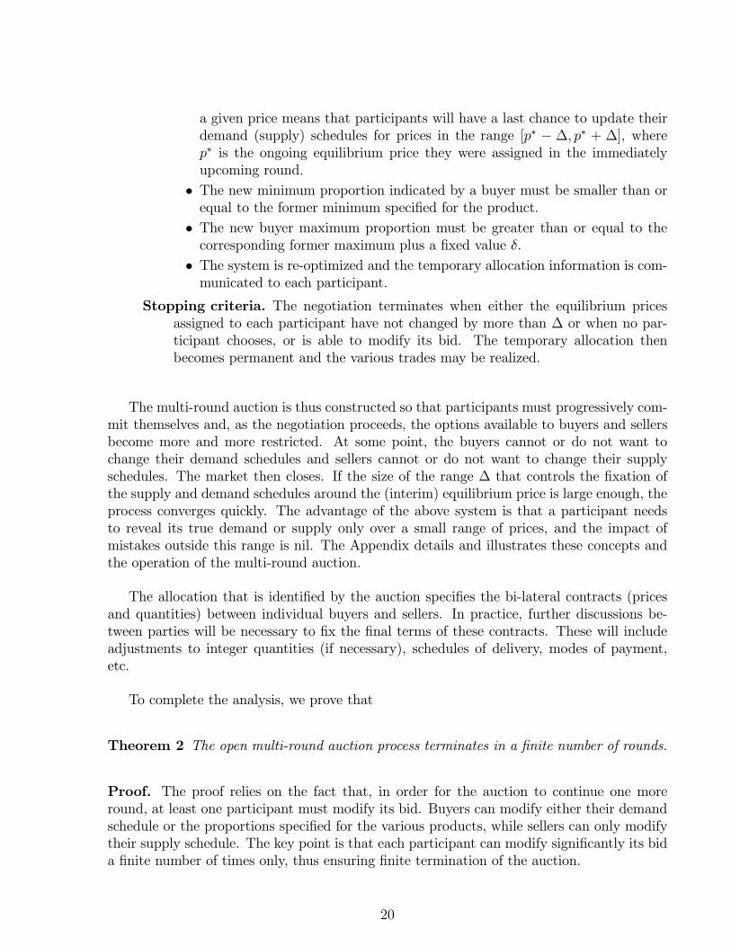
Stopping criteria. The negotiation terminates when either the equilibrium pricesassigned to each participant have not changed by more than ∆ or when no par-ticipant chooses, or is able to modify its bid. The temporary allocation thenbecomes permanent and the various trades may be realized.

The multi-round auction is thus constructed so that participants must progressively com-mit themselves and, as the negotiation proceeds, the options available to buyers and sellersbecome more and more restricted. At some point, the buyers cannot or do not want tochange their demand schedules and sellers cannot or do not want to change their supplyschedules. The market then closes. If the size of the range ∆ that controls the fixation ofthe supply and demand schedules around the (interim) equilibrium price is large enough, theprocess converges quickly. The advantage of the above system is that a participant needsto reveal its true demand or supply only over a small range of prices, and the impact ofmistakes outside this range is nil. The Appendix details and illustrates these concepts andthe operation of the multi-round auction.

The allocation that is identified by the auction specifies the bi-lateral contracts (pricesand quantities) between individual buyers and sellers. In practice, further discussions be-tween parties will be necessary to fix the final terms of these contracts. These will includeadjustments to integer quantities (if necessary), schedules of delivery, modes of payment,etc.

To complete the analysis, we prove that

Theorem 2 The open multi-round auction process terminates in a finite number of rounds.

Proof. The proof relies on the fact that, in order for the auction to continue one moreround, at least one participant must modify its bid. Buyers can modify either their demandschedule or the proportions specified for the various products, while sellers can only modifytheir supply schedule. The key point is that each participant can modify significantly its bida finite number of times only, thus ensuring finite termination of the auction.

20

Regarding product proportions, these range between 0 and 1 and must always be modifiedin a monotonous fashion by at least a fixed amount δ. There can thus be only a limitednumber of such changes.

As for schedules, the schedule for buyer j is fixed in the initial round outside the range[0, c0j(0)], where c

0j(0)] denotes the maximum price declared by this buyer. In subsequent

rounds, the demand schedule becomes fixed for intervals [p∗j −∆, [p∗j +∆], where p∗ standsfor the ongoing equilibrium price assigned to buyer j. At a given iteration, a buyer canchange its schedule around p∗ or for other prices. If the change made is not for p∗ and noother participant changes its bid, this change will be unsignificant and the same equilibriumsolution will be obtained in the next round. This would precipitate the termination of theauction process under the first termination criterion. On the other hand, the buyer canchange its bid quantity for p∗ only if it falls outside a previously fixed range of the schedule,i.e., if it falls in the range [0, c0j(0)] and it differs from previously assigned equilibrium pricesby at least ∆. It is easily remarked that this situation can occur at most (bc0j(0)/∆c + 1)times, since one can place at most (bL/∆c + 1) points spaced ∆ units away in an intervalof length L. Each buyer can therefore make only a limited number of significant changes toits demand schedule.

The reasoning for supply schedules is the same, given the fact that, in the initial round thesupply schedule for lot l is fixed outside the range [0, c0l(Q

l)], where c0l(Ql)] is the maximum

price declared by for lot l. Q.E.D.

It is important to note that the proof above does not depend on whether or not theparticipants declare truthfully their bids. The rules defined above for the multi-round auctionwill always lead to a finite auction process.

5 Applications and Discussion

Wood chip trading in the Province of Quebec is an example of a multi-lateral market withstrong product complementarities, proprietary recipes, geographically dispersed sellers andbuyers, and high transportation costs. It offered us the initial motivation for the workpresented in this paper. Using confidential data on the actual exchanges among wood chipproducers and buyers, we have run simulations in order to estimate the potential cost savingsattainable through the use of an optimized market. In the following, we present and discussthe results of these simulations, examine the issue of the strategic analysis of the associatedmarket game, and examine challenges related to the implementation of optimized markets.

21

5.1 Simulation Analyses

Wood chips are a by-product of the production of lumber wood and the major input inthe production of paper pulp. The annual sales of wood chips from saw mills to paper millsamounts to some 600M$CND in the Province of Quebec alone. Transportation costs accountfor some 20% of the final wood chip cost. The wood chip market is a multi-product market.Saw mills harvest trees, often of different species. Trees are transformed into lumber wood.The excess wood (wood chips) is retrieved and shipped to paper mills. In a given shipment,wood chips from different species are usually mixed up. On arrival at paper mills, wood chipsare weighted and controlled for quality and humidity, and are then stocked according to theirfiber content. It is important to note that most (but not all) buyers need to combine theright proportion of high-density and low-density fibers to respect their specific pulp paperrecipes. Variations in the proportion of high and low-density fibers reduce the quality of thepaper produced. Since buyers typically do not get their wood chips from one source only,they usually combine chips and fibers from different sources for each type of paper produced.There is thus a clear benefit to design auctions that allow bidders to put together efficientcombinations of products at the lowest total acquisition and transportation cost.

We have used 1997 data provided by the Quebec Department of Natural Resources forthe simulations presented herein. The data includes the exact trades in ton between eachpair of buyer and seller. In order to calculate the transportation cost between each sellerand each producer, we have used a matrix containing the distance in kilometers betweeneach paper mills and saw mills and applied the ongoing market price of 0.11$CND per tonper kilometer. Overall 5,79 million tons were traded betweeen 156 saw mills and 33 papermills. The total cost for transporting these tons (based on the assumption of an average costof 0.11$ per ton per kilometer) was 119,4M$CND or an average of 20,63$ per ton, each tontravelling an average of 187,5 kilometers.

Simulations are conducted assuming all necessary information is available and that nomulti-round auction is required. For each simulation, we generate for each seller and buyer asupply or demand curve. The individual supply curves for each saw mill are generated so thatthe quantity supplied at price 100$ corresponds to the actual purchased quantity. Similarly,the individual demand curves for each paper mill are generated so that the quantity askedfor at price 100$ plus their average transportation cost corresponds to the actual purchasedquantity. Hence, the actual trades lie on the respective demand and supply curves. Someassumptions were made for the demand and supply elasticities. However, the elasticityassumptions had little effects on the results of the simulations.

For the first set of simulations, we assumed that all units are equivalent and that thepaper mills are indifferent over the sources of their fibre. These simultations yielded anupper bound on the savings that can be acheived by reallocating trades in the absence ofconstraints on the particular mixtures of wood chips required by buyers. For the secondset of simulations, we assumed that each buyer desires to maintain the same proportions offibres as currently. Estimates of the proportions of high-density, low-density fibers, and grey

22

pine fiber sold by each saw mill depend of the origin region of the lumber and were available.Hence, we could estimate the proportion high-density, low-density fibers, and grey pine fiberpurchased by each paper mill. We imposed that these proportions be preserved. Since, inpractice, paper mills are somewhat more flexible, these simultations establish a lower boundon the savings that can be acheived by reallocating trade. The results of the simulationsfor the entire Qubec market are presented in the Table 2. Quantities are in tons, prices inCanadian dollars.

Quebec Actual trade Simulation I Simulation II(1997) 1 fibre type 3 fibre types

Traded Quantities 5 788 459 5 790 828 5 789 938Average price / ton 100 101,04 100,13Total transportation cost 119 431 175 99 989 592 100 249 121Transportation cost / ton 20,63 17,27 17,31

Table 2: Simulations of Entire Market

Results show overall savings of around 16% in transportation costs per ton. These savingscorrespond to around 19M$. Results do not vary significantly from Simulation I to SimulationII. The average price per ton displayed in the table corresponds to the price received by theproducers. Consequently, compared to the actual trade, producers receive a marginaly higherprice, while buyers pay on average somewhat lower prices as transportation costs go down.The results show that savings are shared by producers and buyers, the buyers receiving mostof the saving in Simulation II.

It is not unreasonable to envision that it could be difficult to bring all the mills of Qubecinto a unique market. Therefore, we have simulated a smaller region and number of firms andexplored the potential savings in this case. We used data from the five paper mills and theirsuppliers within the region of Gaspesia, a remote region in Eastern Qubec. We have fixedthe trade flows among these firms and those outside the region and considered exclusivellythe reallocation of trade within the region. Table 3 presents the results of these simulations.Only the data related to the trade within the region is presented. Similar results to theprevious experiment are observed. Savings around 18% to 19% in transportation cost perton are observed. Compared to the benchmark, producers receive a higher price. Buyerspay on average lower prices in Simulation I but higher prices in Simulation II as savings intransportation costs are upset by the increase in the price paid to producers.

5.2 Strategic Analysis of the Market Game

From a game-theoretical point of view, the process defined by the rules presented in thispaper is hard to analyze. Actually, there is no formal theory about how players interact in adouble-sided market with decreasing demand curves and increasing supply curves. However,there are a few known things about this type of games that allow us to address a number

23

Gaspesia region Actual trade Simulation I Simulation II(1997) 1 fibre type 3 fibre types

Traded Quantities 462 072 462 476 462 478Average price/ton 100 102,15 104,3Total transportation costs 6 921 387 5 579 154 5 694 075Transportation costs / ton 14,97 12,06 12,31

Table 3: Simulations of Restricted Market

of design issues. The main issue is whether the proposed design indeed leads to an efficientallocation of resources and, if not, whether there exist alternative designs that are preferable.

The mechanism proposed in this paper leads to the efficient allocation, if the followingconditions hold: (i) participants truthfully reveal their preferences (cost and demand func-tions, transportations costs, quality evaluation) and (ii) their preferences can be representedwithin the restrictions imposed by our design. Regarding the latter, we believe that for mostcommodity markets, marginal costs are increasing while marginal user values are decreasing.When the representation of preferences and cost structures does not match what is proposedin this paper, the design can be modified. An extreme example is offered by the electricitymarket where significant non-convexities exist in the production functions. In this case, wewould have to modify both the operations research methodology used to optimize the marketand the rules defining how bids may be modified. Most markets do not present such extremeconditions, however, and the required design modifications, if any, are much more benign.

The first condition is more troublesome and, in general, one cannot assume it. In partic-ular, when participants are strategic and large enough to have an impact on the equilibriumprices, then revealing one’s true demand or supply schedule is a dominated strategy. It iswell known that demand (or supply) reduction is a best response against a downward slop-ping excess demand curve (Ausubel and Cramton 1996). If one reduces its demand at themargin, it reduces the price one needs to pay on all sub-marginal units. At the margin, thebenefit of lowering the price outweighs the cost of buying fewer marginal units. Demandreduction and supply reduction leads to fewer trade than what will be socially optimal and,clearly, there will be unexhausted trade gains in the market.

This discussion raises two new questions: (i) to what extent the welfare loss is importantand (ii) does there exist alternative mechanisms that will do better? It appears that nodefinitive answers to these questions exist. The extent of the welfare loss depends on thedegree of competition. If the market is perceived as very competitive, the participants will notbe able to impact prices much and will tend to limit supply and demand reduction. Similarly,it is hard to imagine that one alternative rule will always do better in all circumstances.However, we know that a mechanism that always implements the efficient allocation mustgenerate negative expected returns to the auctioneer (Myerson and Satterthwaite 1983). Inother words, a practical mechanism that always induces efficiency simply does not exist. Onemay consider alternative multi-round auction processes, different pricing rules, or sequential

24

trading mechanisms, the issues of bid and market manipulation will arise still.

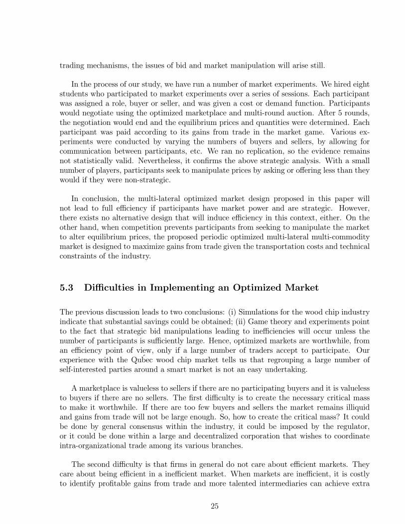
In the process of our study, we have run a number of market experiments. We hired eightstudents who participated to market experiments over a series of sessions. Each participantwas assigned a role, buyer or seller, and was given a cost or demand function. Participantswould negotiate using the optimized marketplace and multi-round auction. After 5 rounds,the negotiation would end and the equilibrium prices and quantities were determined. Eachparticipant was paid according to its gains from trade in the market game. Various ex-periments were conducted by varying the numbers of buyers and sellers, by allowing forcommunication between participants, etc. We ran no replication, so the evidence remainsnot statistically valid. Nevertheless, it confirms the above strategic analysis. With a smallnumber of players, participants seek to manipulate prices by asking or offering less than theywould if they were non-strategic.

In conclusion, the multi-lateral optimized market design proposed in this paper willnot lead to full efficiency if participants have market power and are strategic. However,there exists no alternative design that will induce efficiency in this context, either. On theother hand, when competition prevents participants from seeking to manipulate the marketto alter equilibrium prices, the proposed periodic optimized multi-lateral multi-commoditymarket is designed to maximize gains from trade given the transportation costs and technicalconstraints of the industry.

5.3 Difficulties in Implementing an Optimized Market

The previous discussion leads to two conclusions: (i) Simulations for the wood chip industryindicate that substantial savings could be obtained; (ii) Game theory and experiments pointto the fact that strategic bid manipulations leading to inefficiencies will occur unless thenumber of participants is sufficiently large. Hence, optimized markets are worthwhile, froman efficiency point of view, only if a large number of traders accept to participate. Ourexperience with the Qubec wood chip market tells us that regrouping a large number ofself-interested parties around a smart market is not an easy undertaking.

A marketplace is valueless to sellers if there are no participating buyers and it is valuelessto buyers if there are no sellers. The first difficulty is to create the necessary critical massto make it worthwhile. If there are too few buyers and sellers the market remains illiquidand gains from trade will not be large enough. So, how to create the critical mass? It couldbe done by general consensus within the industry, it could be imposed by the regulator,or it could be done within a large and decentralized corporation that wishes to coordinateintra-organizational trade among its various branches.

The second difficulty is that firms in general do not care about efficient markets. Theycare about being efficient in a inefficient market. When markets are inefficient, it is costlyto identify profitable gains from trade and more talented intermediaries can achieve extra

25

profits. So, naturally, firms invest a lot in market knowledge that could potentially providethem with a competitive advantage. They are unlikely then to move towards a marketenvironment that would render their investment obsolete. One feature of an efficient marketis that information on equilibrium prices is readily accessible, lowering bilateral negotiationcosts. In our discussion with the paper mills, they clearly stated that they did not want tojoin a marketplace, optimized or not, that would provide information on prices. Accordingly,the operator of an electronic marketplace would have a better business model, if it offersa simple trading device (where eventually the negotiated prices remain known only to theinvolved parties) and offers added value services to each individual participant that wishesto pay an extra fee for improved marketing services. Such an offering remains far from theso-called optimized markets.

Despite these previous comments, we believe that the concept of optimized markets willprove fruitful in the long run. Business-to-business electronic commerce seems to moveprogressively towards a more collaborative environment where firms seek to optimize theirjoint efficiency and supply chain. A centralized optimized market may serve as a way toachieve this. When markets remain decentralized, a centralized optimized market modelmay serve as a useful benchmark. Decentralized optimized market mechanisms can also bedeveloped. But these developments are well beyond the scope of the present paper.

6 Conclusions

We presented a design for an optimized, centralized, multi-lateral, periodic commodity mar-ket where all possible multi-lateral trades are solved simultaneously. Commodities are nonhomogeneous and are classified by type or quality. Sellers may offer several commodity typesseparately or mixed up in lots. Buyers need to combine different grades and qualities and,consequently, have to trade with several buyers. Since the complementary commodities areneeded as input to the same process, these trades have to be performed simultaneously.Technological constraints limit the quantities of each type of commodity a buyer may ac-quire. Transportation costs are significant but commodities do not have to pass through ahub on their way from sellers to buyers.

The market clearing mechanism includes explicit optimization tools that seek to allocateresources efficiently, that is to optimize both the production and transportation of resourcesin the industry. Given the information available, the market mechanism identifies an “opti-mal” allocation, which indicated who sells what what to whom, as well as prices, who payswhat to whom. We have detailed the operations research models and the mathematicalprogramming methods required for the efficient computation of the market equilibrium

Since industry participants are usually unwilling or unable to disclose all the pertinentbut very personal and proprietary information required for such an optimized market, we alsointroduced a multi-round auction process that requires significantly less a priori information

26

and allows participants to alter their selling or buying offers in light of the market informationand their own assessment of the market. At each round, the auction makes use of theoptimization procedure to produce a temporary set of allocations and prices. The processcontinues until no one wishes to alter its bid and the efficient bilateral exchanges thenbecome official. Bid changes from one round to the next are governed by eligibility ruleswhose function is to give impetus to the market by prompting participants to be active inthe market and reveal their real needs as early as possible.

The work presented in this paper has shown that building optimized market mechanismsfor complex, multi-lateral, multi-commodity trade is feasible and may be very profitable.Of course, appropriate economic conditions have to exist for firms to desire to join sucha market. We strongly believe such conditions are emerging in a continuously increasingnumber of economic sectors. The methodology proposed may then become the foundationof advanced market mechanisms for those sectors.

Acknowledgments

This project was supported by the Ministry of Natural Resources of Quevec, Bell CanadaUniversity Laboratories, NSERC Canada, the Fonds FCAR of the Province of Quebec, andCIRANO.

References

Abrache, J., Crainic, T.G., and Gendreau, M. (2001). Design Issues for Multi-object Combi-natorial Auctions. In Proceedings of The Fourth International Conference on ElectronicCommerce Research (ICECR-4), volume 2, pages 412—423. Cox School of Business,Southern Methodist University, Dallas TX.

Ausubel, L.M. and Cramton, P. (1996). Demand Reduction and Inefficiency in Multi-UnitAuction. Working paper, University of Maryland.

Bourbeau, B. (1998). Marche periodique optimise: Module d’optimisation. Rapport,CIRANO, Montreal, Canada.

Brewer, P.J. and Plott, C.R. (1996). A Binary Conflict Ascending Price (BICAP) Mechanismfor the Decentralized Allocation of the Right to Use Railroads Tracks. InternationalJournal of Industrial Organization, 14:857—886.

Cramton, P. (1998). Ascending Auctions. European Economic Review, 42:745—756.

De Vries, S. and Vohra, S. (2001). Combinatorial Auctions: A Survey. to appear INFORMSJournal on Computing.

27

DeMartini, C., Kwasnica, A.M., Ledyard, J.O., and Porter, D.P. (1999). A New and Im-proved Design for Multi-object Iterative Auctions. Social Science Working Paper SSWP1054, Caltech.

Fan, M., Stallaert, J., and Whinston, A.B. (1999). A Web-based Financial Trading System.IEEE Computer, 32(4):64—70.

Grether, D.M., Isaac, R.M., and Plott, C.R. (1989). The Allocation Of Scarce Resources:Experimental Economics and the Problem of Allocating Airport Slots. Westview PressUnderground Classics in Economics Series.

Kalagnanam, J.R., Davenport, A.J., and Lee, H.S. (2001). Computational Aspects of Clear-ing Continuous Call Double Auctions with Assignment Constraints and Indivisible De-mand. Electronic Commerce Research, 1(3):221—238.

Ledyard, J.O., Porter, D., and Rangel, A. (1994). Using Computerized Exchange Systemsto Solve an Allocation Problem in Project Management. Journal of OrganizationalComputing, 4(3):271—296.

MacKie-Mason, J.K. (1997). A Smart Market for Resource Reservation in a Multiple Qualityof Service Information Network. Technical report, University of Michigan.

MacKie-Mason, J.K. and Varian, H.R. (1995). Pricing Congestible Network Resources. IEEEJournal of Selected Areas in Communications, 13(7):1141—1149.

Marron, D.B. and Bartels, C.W. (1996). The Use of Computer-Assisted Auctions for Allo-cating Tradable Pollution Permits. In Clearwater, S., editor, Market-Based Control: AParadigm for Distributed Resource Allocation. World Scientific Pub. Co., New York.

Miller, R. (1996). Smart Market Mechanisms: From Practice to Theory. Journal of EconomicDynamics and Control, 20:967—978.

Myerson, R.B. and Satterthwaite, M. (1983). Efficient Mechanisms for Bilateral Trading.Journal of Economic Theory, 28:265—281.

Rassenti, S.J., Smith, V.L., and Bulfin, R.L. (1982). A Combinatorial Auction Mechanismfor Airport Time Slot Allocation. Bell Journal Of Economics, 13(2):402—417.

Rothkopf, M.H., Kahn, E.P., Teisberg, T.J., Eto, J., and Nataf J.-M. (2090). DesigningPurpa Power Purchase Auctions: Theory and Practice. In Plummer, J. and Troppmann,S., editors, Competition in Electricity: New Markets and New Structures, pages 139—194.Public Utilities Reports, Inc., Arlington, VA.

Rothkopf, M.H., Pekec, A., and Harstad, R.M. (1998). Computationally Manageable Com-binatorial Auctions. Management Science, 44:1131—1147.

Sandholm, T. (1999). An Algorithm for Optimal Winner Determination in CombinatorialAuctions. In Proceedings of the International Joint Conference on Artificial Intelligence,pages 542—547.

28

Wilson R. (1997a). Activity Rules for the Power Exchange. Report, The California Trustfor Power Industry Restructuring.

Wilson R. (1997b). Activity Rules for the Power Exchange; Experimental Testing. Report,The California Trust for Power Industry Restructuring.

Appendix

This Appendix details the multi-round auction presented in Section 4. To keep the presen-tation simple, we do not detail the computation of the range ∆ controlling the fixation ofthe demand and supply schedules at each round.

The Preliminary Phase

The preliminary phase initiates the whole process and offers the opportunity to publiclyexchange technical information and to determine the transportation costs. Sellers first an-nounce their technical specifications and their unit transportation costs, that is, the coststhey will have to sustain if they themselves had to handle the transportation of the com-modities sold to buyers, regardless of the transportation mode or carrier used. Buyers thendisclose their quality adjustment factors, calculated on the basis of the seller technical spec-ifications. A second round may then be performed to make the final adjustments to thetechnical specifications and evaluations. This round also offers the opportunity to buyers,sellers, and carriers to compete to offer the best transportation costs between buyers andsellers. As an output of this pre-negotiation phase, the market obtains three sets of infor-mation.

1. The list of commodities K, the set of lots L, as well as the composition of each lotl ∈ L in term of these commodities. This information is provided by sellers.

2. From each buyer j ∈ J , its quality adjustment factors rlj and slj for each lot l ∈ L.3. The matrix of transportation costs tlj indicating the cost of moving one unit of lot l ∈ Lfrom the location of its seller to that of its buyer j ∈ J .

The Initial Bids

Buyers and sellers submit their initial bids that determine the backbone of the computationof the allocation in this and all subsequent rounds.

29

Each buyer must provide a demand schedule, that is, a series of <price, quantity> pairsindicating the number of commodity units (all products) desired and the correspondingprice. Prices must be sorted in descending order, while the associated quantities must bein ascending order. Table 4 illustrates a buyer demand schedule. Prices are the buyer’sacquisition prices and include transportation costs, regardless of who actually pays for theservice. The initial buyer bid must also specify the minimum and maximum proportions ofeach product they wish to obtain in the total quantity they plan to acquire.

Unit Price Quantity Commodity Minimum % Maximum %130 10000 Product 1 50 70125 20000 Product 2 20 50120 30000 Product 3 0 20107 48000

Table 4: Initial Buyer Bid: Demand Schedule and Recipe Table

Using the data in Table 4 as an example, a demand schedule is interpreted as follows(the recipe table is self-explanatory):

1. At a price of 130$, the buyer asks for 10 000 units;

2. At a price between 125$ and 130$, the buyer is ready to buy a quantity between 10000 and 20 000 units;

3. At a price of 125$, the buyer would buy 20 000 units;

4. At a price between 120$ and 125$, the buyer is ready to by between 20 000 and 30 000units; and so on for the subsequent prices;

5. At a price below 107$, the buyer always asks for 48 000 units, which represents itsmaximum demand. By convention, and without the buyer having to specify it, thesystem creates the <price, quantity> pair <0, 48 001> to incorporate the informationdisclosed by the buyer whereby a price below 107$ will have no significant impact onthe quantity it is ready to acquire.

Sellers provide their supply schedules, or bids, one for each lot they want to sell. A supplyschedule is made up of a number of pairs <price, quantity>, both prices and quantities beingordered in ascending order. Table 5 illustrates a seller supply schedule. It is interpreted asfollows:

1. At a price below 80$, the seller offers nothing; by convention, and without the sellerhaving to specify it, the system will create the <price, quantity> pair <79, 0> toincorporate the information disclosed by the seller whereby 80$ is the minimum priceat which it is prepared to sell;

30

2. At a price of 80$, the seller offers 5 000 units;

3. At a price between 80$ and 85$, it is ready to sell between 5 000 and 7 000 units;

4. At a price of 85$, the seller offers 7 000 units;

5. At a price between 85$ and 90$, the seller offers between 7 000 and 8 000 units; andso on for the subsequent prices;

6. At a price above 100$, the seller offers 10 000 units, its maximum supply or productioncapacity. By convention, and without the seller having to specify it, the system createsthe <price, quantity> pair <P, 10 001>, where P is an arbitrarily high price, toincorporate the information disclosed by the seller whereby raising the price above100$ will have no significant impact on the quantity it offers.

Unit Price Quantity80 500085 700090 8000100 10000

Table 5: Initial Seller Bid: Supply Schedule

The first round ends when all buyer and seller bids have been received, or at a pre-determined time. A temporary market allocation and prices are then computed by theoptimization methodology.

Market Optimization and Allocation

In each round, once bids have been submitted or modified, the system calculates optimalallocations (prices and quantities) to maximize the efficiency of the market based on cur-rent information. Buyer utility and seller production cost functions are derived from cur-rent demand schedules and supply schedules, respectively, by connecting the given <price,quantity> points by straight lines. This, plus the required ordering of the schedules ensuresthe desired properties of the functional forms. This information is completed by the currentbuyers’ recipes and the constant data, namely the transportation costs and the technicalrequirements.

The optimized market allocated model (Section 2) is then solved by the quadratic op-timization method of Section 3. The output of this process, the optimal quantities of lot lsold to buyer j, ql∗j and the associated equilibrium prices p

l∗j , make up the temporary market

allocation that will become permanent if no buyer or seller desires to modify its bid.

31

The system communicates the market information to each participant, but each buyerand sellers receives only the information that targets it directly:

Seller: Separate quantities and equilibrium prices for each lot offered;

Buyer: Quantities and equilibrium prices for each lot purchased, the weighted average ofthese prices, and the sum of all quantities obtained;

Non-participating seller: For the non-participating lots, the price to sell a minimal quan-tity, or an indication that the technical characteristics of the lot do not match thebuyers’ requirements;

Non-participating buyer: The minimum price at which it may acquire some small quan-tity, or an indication that its technical requirements are non compatible with the lotson sale.

Unit Price Quantity Commodity Quantity Average Price130 10000 Product 1 17500 121.57125 20000 Product 2 5000 128

122.5 25000 Product 3 2500 118120 30000 Total 25000 122.5107 48000

Table 6: Example of Information Received by the Buyer After the First Round

To illustrate, consider the case of a buyer whose initial bid is given by Table 5. If itstemporary average equilibrium price, for all commodities, is 120$, then the total quantity itreceives is 30 000 units. Obviously, most of the time, the average equilibrium price will notcoincide with a point already in the demand schedule. Then, the total quantity obtainedis computed according to the line segment of the demand schedule to which the averageprice belongs. Thus, for an average equilibrium price of 122.50$, which belongs to the linesegment <120, 20 000> - <125, 30 000>, a total quantity of 25 000 units will be allocated tothe buyer. A new <price, quantity> pair is then added to the demand schedule to indicatethe price and the equilibrium quantity in this particular case (illustrated in Table 6) andfurther refine the approximation of the utility curve of the buyer. Similar manipulations areperformed on seller supply schedules. Note that prices announced to buyers are not be thesame as those announced to sellers, in particular because the latter include the transportationcosts. Based on this information, buyers and sellers may modify their bids as described inthe next subsection.

Bids in Subsequent Rounds

Once the first round allocations are known, buyers and sellers may be interested in alteringtheir bids. Upon the announcement of the start of a new round, participants are authorized

32

to alter their demand or supply schedules. Buyers may also alter their recipe tables. Around ends when the equilibrium prices assigned to each participant have not changed bymore than ∆, at a pre-set time, when all bids have been received, or if no bid modificationsare recorded within a pre-set period. The temporary allocation then becomes permanentand the various trades may be realized.

In an auction process involving successive rounds, it is essential to establish eligibilityrules. These rules aim to give impetus to the market. The idea is to avoid dragging out thenegotiation because “participants” merely watch the market and wait for too long beforeintervening. Eligibility rules also aim to guide the way participants may modify their bids.The goal here is to ensure that the multi-round auction will eventually “converge”. Whentechnological constraints are involved, as in the present case, one also desires to make surethat modifications to these ensure that previous allocations are still feasible. We thus imposeseveral restrictions on bid modification for the auction mechanism we propose (these rulesare quite similar to those proposed in Wilson 1997a, 1997b)):

1. A participant may only raise its bid. That is, at any given price, a buyer or seller mayonly increase the quantities submitted previously;

2. Demand schedules are strictly decreasing in price and increasing in quantity, whilesupply schedules are strictly increasing in both price and quantity;

3. In each round, one new point of the demand (supply) schedule is fixed permanently.In the initial round, it is the point of the demand (supply) schedule with the highestquantity (the lowest price for buyers, the highest price for sellers). In all subsequentperiods, it will be the point associated with (or around) the ongoing equilibrium pricethat will be fixed for the rest of the negotiation;

4. The new minimum proportion indicated by a buyer must be smaller than or equal tothe former minimum specified for the product;

5. The new buyer maximum proportion must be greater than or equal to the correspond-ing former maximum.

The multi-round auction is thus constructed so that participants must progressively com-mit themselves. In the initial round, for example, the last row of a buyer demand scheduleis fixed for ever. This means, the buyer will never be allowed to ask for more than thequantity it initially requested at the lowest price. Because the demand schedule is strictlydecreasing in price and increasing in quantity, the buyer may never demand more at anyother price either. For a buyer for whom Table 5 represents the first round bid, the maxi-mum eligibility quantity is set at 48 000, for all prices. Now, suppose that after round 1, theauctioneer estimates an (interim) equilibrium price of 122.5$ and provides the buyer withthe information displayed in Table 6. The mechanism is thus asking the buyer to commit toa quantity for the price 122.5$, for the rest of the negotiation. Since demand in decreasingin price, the buyer will not be allowed to ask for a greater quantity at prices equal or below

33

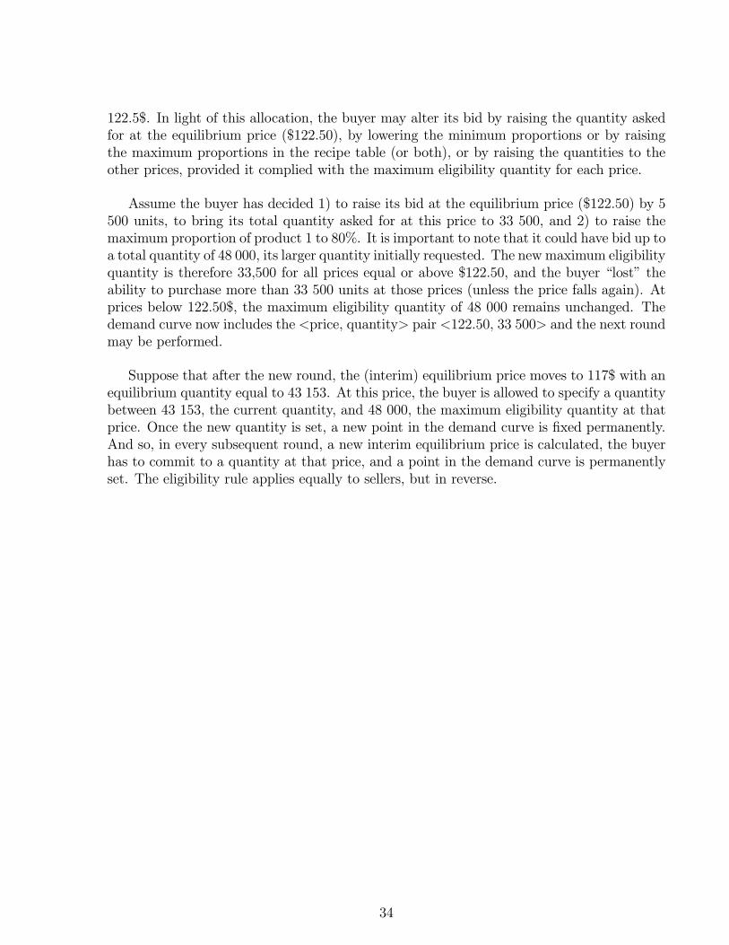
122.5$. In light of this allocation, the buyer may alter its bid by raising the quantity askedfor at the equilibrium price ($122.50), by lowering the minimum proportions or by raisingthe maximum proportions in the recipe table (or both), or by raising the quantities to theother prices, provided it complied with the maximum eligibility quantity for each price.

Assume the buyer has decided 1) to raise its bid at the equilibrium price ($122.50) by 5500 units, to bring its total quantity asked for at this price to 33 500, and 2) to raise themaximum proportion of product 1 to 80%. It is important to note that it could have bid up toa total quantity of 48 000, its larger quantity initially requested. The new maximum eligibilityquantity is therefore 33,500 for all prices equal or above $122.50, and the buyer “lost” theability to purchase more than 33 500 units at those prices (unless the price falls again). Atprices below 122.50$, the maximum eligibility quantity of 48 000 remains unchanged. Thedemand curve now includes the <price, quantity> pair <122.50, 33 500> and the next roundmay be performed.

Suppose that after the new round, the (interim) equilibrium price moves to 117$ with anequilibrium quantity equal to 43 153. At this price, the buyer is allowed to specify a quantitybetween 43 153, the current quantity, and 48 000, the maximum eligibility quantity at thatprice. Once the new quantity is set, a new point in the demand curve is fixed permanently.And so, in every subsequent round, a new interim equilibrium price is calculated, the buyerhas to commit to a quantity at that price, and a point in the demand curve is permanentlyset. The eligibility rule applies equally to sellers, but in reverse.

34