2001 Modeling and control of a flexible-link manipulator

Lakehead University

Knowledge Commons,http://knowledgecommons.lakeheadu.ca

Electronic Theses and Dissertations Retrospective theses

2001

Modeling and control of a flexible-link manipulator

McDonald, Brandeen Ann

http://knowledgecommons.lakeheadu.ca/handle/2453/3180

Downloaded from Lakehead University, KnowledgeCommons

INFORMATION TO USERS

This manuscript has been reproduced from the microfilm master. UMi films the text directly from the original or copy submitted. Thus, some thesis and dissertation copies are in typewriter face, while others may be from any type of computer printer.

The quality of this reproduction is dependent upon the quality of the copy submitted. Broken or indistinct print, colored or poor quality illustrations and photographs, print bleedthrough, substandard margins, and improper alignment can adversely affect reproduction.

In the unlikely event that the author did not send UMI a complete manuscript and tfiere are missing pages, these will be noted. Also, if unauthorized copyright material had to be removed, a note will indicate the deletion.

Oversize materials (e.g., maps, drawings, charts) are reproduced by sectioning the original, beginning at the upper left-hand comer and continuing from left to right in equal sections with small overlaps.

Photographs included in the original manuscript have been reproduced xerographically in this copy. Higher quality 6” x 9" black and white photographic prints are availat)le for any photographs or illustrations appearing in this copy for an additional charge. Contact UMI directly to order.

ProQuest Information and Leaming 300 North Zeeb Road, Ann Arbor, Ml 48106-1346 USA

800-521-0600

UMI

Reproduced with permission of the copyright owner. Further reproduction prohibited without permission.

Reproduced with permission of the copyright owner. Further reproduction prohibited without permission.Reproduced with permission of the copyright owner. Further reproduction prohibited without permission.

Modeling and Control of a Flexible-LInk Manipulator

Brandeen McDonald ® August 14, 2001

A THESIS SUBMITTED IN PARTIAL FULFILLMENT OF THE REQUIREMENTSOF THE MScEng DEGREE

INCONTROL ENGINEERING

FACULTY OF ENGINEERING LAKEHEAD UNIVERSITY

THUNDER BAY, ONTARIO CANADA


1 * 1National Library of Canada

Acquisitions and Bibliographic Sen/ices395 Waffington Street Ottawa ON K1A0N4 Canada

Bibliothèque nationale du Canada

Acquisitions et services bibliographiques395, rue Wettington Ottawa ON K1A0N4 Canada

Y o u rm Votm réêétwno0

Our A» Notrmr4téimK0

The author has granted a nonexclusive licence allowing the National Libraiy of Canada to reproduce, loan, distribute or sell copies of this thesis in microform, paper or electronic formats.

The author retains ownership of the copyri^t in this thesis. Neidier the thesis nor substantial extracts from it may be printed or otherwise reproduced without the author’s permission.

L’auteur a accordé une Licence non exclusive permettant à la Bibliothèque nationale du Canada de reproduire, prêter, distribuer ou vendre des copies de cette thèse sous la forme de microfîche/fîlm, de reproduction sur papim* ou sur format électronique.

L’auteur conserve la propriété du droit d’auteur qui protège cette thèse. Ni la thèse ni des extraits substantiels de celle-ci ne doivent être imprimés ou autrement reproduits sans son autorisation.

0-612-64726-9

Canada


Abstract

The behaviour o f a flexible-Iink robotic manipulator is studied using an experimental apparatus. The system is modeled based on the physical laws governing system dynamics. A non-linear rigid body model is developed which includes backlash and friction. Through comparison o f experimental and simulation results, the small backlash in the system is shown to have little effect on the system behaviour.

Friction is shown to have a considerable effect on the system dynamics. The finite element method is used to develop a flexible body model for the flexible link. Experimental results show that the lateral vibration o f the manipulator exhibits the behaviour o f a clamped-fi:ee beam or a pinned-fiee beam during different stages o f the motion. A combined dynamic model has been developed. The model is comprised of both a clamped-fiee beam model and a pinned-fiw beam model with the choice o f model being determined by the boundary conditions at the hub that change due to the non-linear fiiction term included in the model.

Experimental and simulation results demonstrate that, at low speeds o f rotation, the hub friction causes the pinned frequencies o f vibration to approach the clamped fi^uencies. Vibration suppression controllers are considered based on the coupling torque from the clamped beam model. Different vibration-suppressing controllers are found to be effective in the pinned, high-speed region, the pirmed, low-speed region and the clamped region. The effectiveness o f vibration-suppressing controllers when added to a classical PD controller is studied.

11


Acknowledgements

I would like to thank Dr. K. Natarajan, my thesis supervisor, for providing direction and guidance. The attention to detail shown by Dr. K. Liu in his examination o f the thesis was very helpful and much appreciated. The assistance and advice from Drs. A. Gilbert, K. Liu and M. Liu were sincerely appreciated. 1 would like to thank F. Briden and B. Misner for their help with the C programming language. My classmate Xiaodong Sun deserves thanks for his thoughtfhl discussion. Liz Tse deserves a special mention for her honest opinions. 1 am very grateful to Lori Kapush for proof reading this woric. My heartfelt gratitude goes to my friends and family for their loving support, and not only believing 1 could do it, but also telling me so.

Ill


Table of Contents

A bstract.............................................................................................................................. iiAcknowledgements ................................................................................~.........................iiiT able of C onten ts_______ ......................................_____________________________ ivList o f Figures ................................................................................................................. vList o f Nom enclature________________________ vii1. In troduction __________ ..............................______________________________ 1

1.1 Why Study Flexible Manipulators..............................................................................11.2 Modeling o f Robotic Arm s......................................................................................... 11.3 Control Strategies........................................................................................................ 31.4 Thesis Overview.......................................................................................................... 3

2. The System Under Study.............................................................................................. 52.1 Rigid Body Model with Backlash and Friction.........................................................62.2 Friction Model............................................................................................................112.3 Comparison o f Simulated and Experimental Data..................................................122.4 Effects o f Flexing on Speed......................................................................................152.5 Conclusions................................................................................................................16

3. System Model Combining Rigid Body and Flexible Arm Dynamics ..................... 173.1 Pinned-Free Beam Model..........................................................................................193.2 Clamped-Free Beam Model..................................................................................... 223.3 Strain Gage Reading Estimation..............................................................................273.4 Experimental and Simulated Results.......................................................................273.5 Conclusions............................................................................................................... 32

4. C ontroller Design_________________________ 334 .1 Controller Design Based on Clamped M odel.........................................................344.2 Controller Design Based on Pinned Model without Friction................................ 384.3 Controller for Pinned Model with Friction............................................................. 394.4 Vibration-suppressing Controller Design for the Complete System.................... 434.5 System Response to PD Control with Added Vibration-suppressing Control.. . 434.6 Conclusions............................................................................................................... 49

5. Conclusions and Future Work.................................................................................. SOReferences........................................................................................................................ 52Appendix A .....................................................................................................................54

Determination o f System Constants............................................................................... 54Experiment 1 : Calculating the Motor Constant............................................................ 54Experiment 2: Determining the Viscous and Coulomb Friction in the Motor andShaft (without position potentiometer)..........................................................................55Experiment 3 : Determining Motor Inertia Based on Run-down Curve Data........... 56Experiment 4: Determining the Viscous and Coulomb Friction o f the SystemIncluding the Flexible Arm............................................................................................. 58Experiment 5 : Determination of Static Friction...........................................................59

IV

Reproduced with permission ot the copyright owner. Further reproduction prohibited without permission.

List of Figures

Figure 2.1 Experimental Setup...................................................................................................6Figure 2.2 The flexible arm system........................................................................................... 6Figure 2.3 Moment o f Inertia o f A rm ....................................................................................... 7Figure 2.4 Forces and torques acting on the gears................................................................... 8Figure 2.5 Friction M odel.........................................................................................................12Figure 2.6 Experimental (top) and simulated (bottom) results. Controller settings

P=2.5308, D = 0.6625. Simulation has backlash and friction...........................13Figure 2.7 Experimental Speed, Simulated speed with backlash. Simulated Speed without

backlash....................................................................................................................14Figure 2.8 Experimental Speed, Simulated speed with backlash. Simulated speed without

backlash. Controller rate has been constrained................................................. 15Figure 2.9 Experimental Speed, Base Gage and Second Gage Measurements...................16Figure 3.1 Experimental Second Gage (V) (green) and Speed (rad/s) (blue) for system

with no payload...................................................................................................... 18Figure 3.2 Beam Deflection in the x-y plane.......................................................................... 19Figure 3.3 Beam Deflection in the x-y plane..........................................................................23Figure 3.4. Positive direction o f reaction torque. Mo at the hub caused by flexing o f the

arm due to applied torque %,..................................................................................25Figure 3.5 Experimental and Pinned-Mode Simulation Results using initial calculated

value o f Jm............................................................................................................... 28Figure 3.6 Experimental and Pinned-Mode Simulation Results using adjusted value o f Jm.

..................................................................................................................................29Figure 3.7 Comparison o f Experimental System and Clamped-Mode Simulation............29Figure 3.8 Comparison o f combined system simulation and experimental results............ 30Figure 3.9 Effect on the combined system simulation caused by adding beam damping to

the pinned m odel....................................................................................................31Figure 3.10 Experimental and simulation results for a payload of300g............................. 31Figure 4.1 Block diagram o f PD plus vibration suppression control................................... 34Figure 4.2 The clamped system model response for Kmo = -I and td = 0............................ 35Figure 4.3 The clamped system model response for Kmo = -1 and td = 0.074 sec.............. 36Figure 4.4 The pinned system model (with fiiction) response for Kmo = -1 and td = 0.026

sec.............................................................................................................................37Figure 4.5 Pinned system model response, for Kmo = -1 and td = 0.026 sec., with current

limited to 5A........................................................................................................... 37Figure 4.6 Experimental system response, for Kmo = -1 and td = 0.026 sec., with current

limited to 5 A ........................................................................................................... 38Figure 4.7 The pinned system model response, for Kmo = -1 and td = 0 sec....................... 39Figure 4.8 The pinned system model (with friction) response, for Kmo = -1 and td = 0 sec.

..................................................................................................................................40Figure 4.9 The pinned system model (with friction) response, for Kmo = -1 and td = 0 sec.

plus low-speed fiiction compensation..................................................................40Figure 4 .10 The pinned system model (with fiiction) response, for Kmo = 1 and td = 0 sec.

.................................................................................................................................. 41


Figure 4 .1 1 The pinned system model (with fiiction) response, for Kmo = 1 and tj = 0 sec,plus low-speed fiiction compensation.................................................................41

Figure 4.12 The pinned system model (with fiiction) response, for Kmo = -1 and td = 0sec., with the controller applied at low speed only.............................................42

Figure 4.13 The pinned system model (with fiiction) response, for Kmo = -1 and td = 0 sec., with the controller applied at low speed only plus low-speed fiictioncompensation..........................................................................................................42

Figure 4.14 Complete system model with a combined controller....................................... 43Figure 4.15 System response to a setpoint o f 100® with PD control................................... 44Figure 4.16 System response with PD and combined controller.........................................44Figure 4.17 Total system with PD control and with vibration-suppressing control in the

low-speed pinned region only...............................................................................45Figure 4.18 Total System with PD Control and with vibration-suppressing control at high

speeds only..............................................................................................................45Figure 4.19 Strain Gage Comparisons.................................................................................... 46Figure 4.20 Experimental System with PD control............................................................... 47Figure 4.21 Experiment response for a PD control with vibration-suppressing control at

h i ^ speed............................................................................................................... 48Figure 4.22 Experiment Strain Gage Comparisons............................................................... 49

VI


List of NomenclatureAO- the gear backlash width, in rad.

the magnetic flux, in Vs.- generalized shape (unctions.

0 i{x) — the slope o f the beam at the hub, in rad.Ozix) — the slope o f the beam at the tip, in rad.Oa - the angle o f the arm gear, in rad.0„ - the angle o f the motor gear, in rad.r - the input to the rigid-flexible body system model.Ta - the torque supplied by the motor current, in Nm.Ti - the torque available to the motor load, in Nm.T2 - the load torque on the arm gear side, in Nm. n*,. - arm speed before gear engagement, in rad/s. atj- the arm speed, in rad/s.

- arm speed after gear engagement, in rad/s.0)n. - motor speed before gear engagement, in rad/s. ain- the motor speed in, rad/s.0*,+ - motor speed after gear engagement, in rad/s.A ^ ,C — the state space matrices.ao, a I, a 2 , 0 3 - coefficients in the beam deflection equation. b - the total viscous fiiction o f the system in Nms b„ - the viscous friction o f the motor in Nms.6j - th e viscous fiiction o f the arm shaft in Nms.B t - the damping matrix for the combined rigid-flexible body system model.D - gain o f the derivative controller. di - the length o f the counter balance, in m.

d2 - the length o f the flexible portion o f the arm, in m. dj - the distance to the payload, in m.£ - the modulus o f elasticity for 6061-T6 aluminum, in Pa.Ea - the back em f o f the motor, in V./ / - the force applied between gears due to torque f/, in N.F2 - generalized force on the tip o f the beam, in N. f 2 - the reaction force between die gears due to / / , in N.Fm - force at the tip o f the beam due to 0„ , in N.Fm - the force on the end o f the beam caused by a payload mass, in N./ - t h e area moment o f inertia o f the arm, in m^./ - t h e identity matrix.ia - the current supplied to the motor, in A.J - the total mass moment o f inertia o f the system, in kgm^Ja - the moment o f inertia o f the arm, arm shaft, arm ^ear and any payload, in kgm". Jgi - the moment o f inertia o f the motor gear, in kgm \Jg2 ’ the moment o f inertia o f the arm gear and shaft, in kgm".

VII


Ji - the moment o f inertia o f the arm including payload, in kgm^.Jm - the moment o f inertia o f the motor and motor gear combined, in kgm^.Jm2 - inertia o f counterbalance, in kgm^.Jm2 - the moment o f inertia o f the counterbalance, in kgm“.Jr - the moment o f inertia o f the motor (rotor), in kgm'. k0 - the motor constant in Nm/A.K b - generalized stiffiiess matrix.kij - the elements o f the generalized stiffiiess matrix, Kb-K„o - gain tuning parameter for vibration suppressing controller.Ksg - gain used in calculating the second strain gage reading.K t ~ the stiffiiess matrix for the combined rigd-flexible body system model.£ - the length o f the beam in m.La - the motor inductance, in henrysM{x) - moment at any point along the beam, in Nm.m(x) - the per unit l e n ^ mass o f the beam, in kg/m.M l - generalized moment at the hub, in Nm.m/ - the mass o f the flexible portion o f the arm, in kg.M 2 - generalized moment on the tip o f the beam, in Nm. m2 - the mass o f the counter balance, in kg. m3 - the mass o f the payload, in kg.M b - generalized mass matrix.MBNo_mass ~~ MB'MBPayioad ~ the generalized mass matrix for the system with payload. mij - the elements o f the generalized mass matrix, Mb- Mm - torque at the tip o f the beam due to , in Nm.Mo - reaction torque at the hub (referred to motor gear side) caused by the flexing o f the arm, in Nm.M t - the mass matrix for the combined rigd-flexible body system model.N - the gear ratio, r / r j .P - gain o f the porportional controller.p{x) - the distributed force on the beam, in N/m.Q - the input matrix for the combined rigd-flexible body system model. ri - the radius o f the motor gear, in m. r , - the radius o f the arm gear, in m.Ra - the motor resistance, in ohms SG ~ second strain gage reading, in V./ — time, in seconds.Taf- the arm shaft fiiction (coulomb and static), in Nm.td - delay tuning parameter for vibration suppressing controller.Tf- the total fiiction in the system, in NmT„f - the motor fiiction (coulomb and static), in Nm.u - the state input.v^Jf) - the deflection o f the beam at the tip, in m.X - the distance along the length o f the beam, in m.X - the state variable.y(x,0 - the deflection o f the beam, in m.

Vlll


Chapter 1

Introduction

1.1 Why Study Flexible Manipulators

The large mass and energy requirements o f standard rigid link manipulators have led to a desire for flexible link manipulators characterized by low-mass links and actuators with low power requirements. TWs is particularly desirable in certain applications, such as space systems, where mass and energy requirements must be minimized for transport purposes. Flexible link dynamics are also found in certain mechanical pointing systems [ 18] and in systems with links having high length-to-width ratios. These dynamics make the system outputs such as tip position more difficult to control. If flexibility is not taken into account in controller design the system can become unstable. Therefore, before flexible link manipulators can be realistically implemented, it is necessary to study the nature o f flexible link manipulators and determine effective methods for end-point position control.

1.2 Modeling of Robotic Arms

Studies on the modeling of flexible robotic arms can be divided into two areas - those that use identification based methods and those that develop models based on the physical laws o f the dynamic system.

Identification based methods are advantageous in that they do not require specific system parameters and therefore can be used on systems that are already built and for which the governing equations are complex or system parameters are unknown and cannot be measured. However, in addition to large computation times, time domain identification based methods require a model order which can be difficult to choose as flexible body dynamics involve partial differential equations. The model order selected therefore usually results in over- or under- parameterization. Frequency domain methods have been used in [22] to avoid these problems associated with time domain identification models.


For systems that use the identified model for controller tuning, sufficient time must be available to update the model and tune the controller. It is shown in [23] that good performance results are obtained irrespective o f payload using online identification and controller tuning. However, the identification and tuning o f the controller is too time consuming to be practical. The FFT is used in [22] to reduce the identification time of the first natural fiiequency o f the system. This mode is used to choose the controller gains in a gain scheduling technique. This significantly reduced the controller tuning time. Since addition o f a payload tends to lower the first natural frequency, this method successfully adapts the controller to payload changes and provides good response to step inputs.

The majority o f studies [8,12,5,2,7,9,3] based on the physics o f the system use Lagrange’s equation to construct a suitable state-space representation and include both rigid body and flexible body components. The energr balance nature of the Lagrangian method naturally includes coupling terms between the rigid and flexible bodies. In [3] however, the linear model is decoupled, and the coefficients o f the state-space model are determined via an identification technique. An experimental technique is used in [11] to identify the fi%quencies o f vibration. However, since it measures the beam vibrations after the arm has been rotated through a slew angle, it only measures the clamped-finee frequencies [10]. Previous methods that use physical modeling techniques chose either clamped-fi-ee or pitmed-fi*ee beam models for the flexible body, and use the corresponding eigenfunctions in the system model development. Results for both cases are compared in [9]. In [20] the eigenfunctions are chosen based on the frame o f reference. This seems to imply that the frequency o f vibration for a beam depends on the frame o f reference. The fi-equency o f vibration depends on the boundary conditions o f the system, not the frame o f reference. A different frame o f reference for a model describing the same system should yield the same results.

In [12] the models from [9] are used and it is mentioned that a system with a higher hub inertia will have frequencies closer to the clamped-free frequencies and a system with lower hub inertia will have fr^equencies closer to the pirmed-free fi-equencies. In [7, 6] the higher gear ratio reduces the effect o f the oscillations o f the arm on the motor and causes vibrations closer to the clamped mode. Such a high gear ratio also prevents a rapid response and therefore requires a motor with higher speed capabilities.

Some studies [5, 7] include terms to account for non-linearities such as Coulomb friction. In [7] the friction term is represented by a linear approximation.

Past studies [11,12,3,5,7] on flexible manipulators have used tip sensors to monitor the tip position and how it reacts to flexing. These include accelerometers that provide indirect estimation o f tip position and video camera techniques that provide tip position for a limited range o f movement. Other researchers [8, 9] have used strain gages to monitor the stress in the flexible link. In this case, when the sensor outputs have reached steady state, the tip position is equal to the hub position.


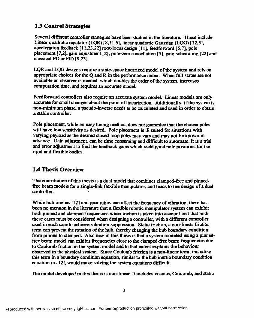
13 Control Strategies

Several different controller strategies have been studied in the literature. These include Linear quadratic regulator (LQR) [8,11,5], linear quadratic Gaussian (LQG) [12,3], acceleration feedback [11,23,22] root-locus design [11], feedforward [5,7], pole placement [7,2], gain adjustment [2], pole-zero cancellation [5], gain scheduling [22] and classical PD or PID [9,23]

LQR and LQG designs require a state-space linearized model o f the system and rely on appropriate choices for the Q and R in the performance index. When full states are not available an observer is needed, which doubles the order o f the system, increases computation time, and requires an accurate model.

Feedforward controllers also require an accurate system model. Linear models are only accurate for small changes about the point o f linearization. Additionally, i f the system is non-minimum phase, a pseudo-inverse needs to be calculated and used in order to obtain a stable controller.

Pole placement, while an easy tuning method, does not guarantee that the chosen poles will have low sensitivity as desired. Pole placement is ill suited for situations with varying payload as the desired closed loop poles may vary and may not be known in advance. Gain adjustment, can be time consuming and difficult to automate. It is a trial and error adjustment to find the feedback gains which yield good pole positions for the rigid and flexible bodies.

1.4 Thesis Overview

The contribution of this thesis is a dual model that combines clamped-fi-ee and piimed- ffee beam models for a single-link flexible manipulator, and leads to the design o f a dual controller.

While hub inertias [12] and gear ratios can affect the frequency o f vibration, there has been no mention in the literature that a flexible robotic manipulator system can exhibit both pinned and clamped frequencies when friction is taken into account and that both these cases must be considered when designing a controller, with a different controller used in each case to achieve vibration suppression. Static friction, a non-linear friction term can prevent the rotation o f the hub, thereby changing the hub boundary condition from pinned to clamped. Also new in this thesis is that a system modeled using a pinned- frree beam model can exhibit frequencies close to the clamped-free beam frequencies due to Coulomb friction in the system model and to that extent explains the behaviour observed in the physical system. Since Coulomb friction is a non-linear term, including this term in a boundary condition equation, similar to the hub inertia boundary condition equation in [ 12], would make solving the system equations difficult.

The model developed in this thesis is non-linear. It includes viscous. Coulomb, and static


fiiction. Both the rigid and the flexible bodies are modeled using the physical laws that govern the system. The equations for the rigid and flexible body motion are derived separately, and then combined. For the clamped model, an explicit reaction term [4,5] is added to couple the two systems. Modeling in this fashion, with an explicit reaction term, allows for the theoretical study of the nature o f the coupling between the rigid and flexible bodies and allows for the design o f a controller which can predict this coupling and reduce its effects on the system. An explicit coupling term caimot be determined for the pinned model. Since the nature of the coupling is different under pinned or clamped conditions, a dual controller is needed.

This thesis also uses strain gages to monitor beam flexing, but differs in that the gages are also used to predict the effects o f flexing on the motor speed and the reaction torque at the hub. The effect o f beam flexing on motor speed and arm position is important since these rigid body variables and the strain gage readings are the only values measured from the experimental system. While the majority of papers with experimental results [3,5,7,6,9,11,1232,23] move the arm th ro u ^ angles ranging from 5 —40 degrees, in this thesis, similar to [21], slew angles of 100 degrees are considered. Rotating the arm through a large angle allows a wider range of behaviours to be observed.

The outline o f this thesis is as follows: Chapter 1 is the introduction. Chapter 2 develops the rigid body model o f the system and explores the contribution o f backlash to system dynamics. Chapter 3 develops the flexible body model o f the system and describes the effects o f fiiction. Chapter 4 shows the results for various control strategies and Chapter 5 gives conclusions and outlines future work.


Chapter 2

The System Under Study

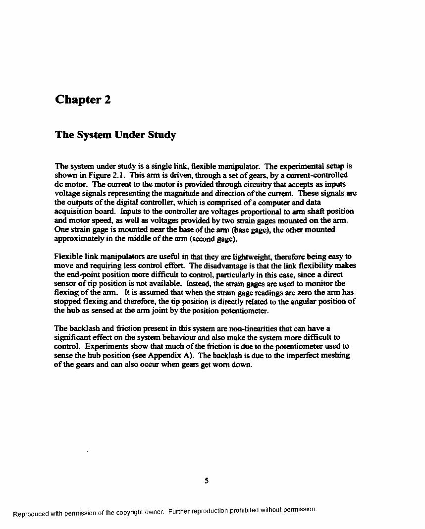
The system under study is a single link, flexible manipulator. The experimental setup is shown in Figure 2.1. This arm is driven, through a set o f gears, by a current-controlled dc motor. The current to the motor is provided through circuitry that accepts as inputs voltage signals representing the magnitude and direction of the current. These signals are the outputs o f the digital controller, which is comprised of a computer and data acquisition board. Inputs to the controller are voltages proportional to arm shaft position and motor speed, as well as voltages provided by two strain gages mounted on the arm. One strain gage is mounted near the base of the arm (base gage), the other mounted approximately in the middle o f the arm (second gage).

Flexible link manipulators are useful in that they are lightweight, therefore being easy to move and requiring less control effort. The disadvantage is that the link flexibility makes the end-point position more difficult to control, particularly in this case, since a direct sensor o f tip position is not available. Instead, the strain gages are used to monitor the flexing o f the arm. It is assumed that when the strain gage readings are zero the arm has stopped flexing and therefore, the tip position is directly related to the angular position o f the hub as sensed at the arm joint by die position potentiometer.

The backlash and friction present in this system are non-linearities that can have a significant effect on the system behaviour and also make the system more difficult to control. Experiments show that much o f the fiiction is due to the potentiometer used to sense the hub position (see Appendix A). The backlash is due to die imperfect meshing o f the gears and can also occur when gears get worn down.


Digital Controller

Single Link Rexible Manipulator

Current Control Circuitry

Position Sensor

DC Motor

Strain Gage Sensor

Motor Current Input

Speed Signal

Figure 2.1 Experimental Setup

2.1 Rigid Body Model with Backlash and Friction

In this section the system is modeled as a rigid body, including the non-linearities o f backlash and fiiction. The backlash width measures the maximum gap between motor gear teeth and arm gear teeth and as such, is the angle, in radians, subtended by the contact surfaces o f the gear teeth at the centre o f the motor gear.

To describe gear backlash, three cases must be described [18]: when the gears are engaged, when the gears are not engaged, and the moment o f impact when the gears engage.

L

Figure 2.2 The flexible arm system.

When the gears are engaged, the system can be described by the general equation:

(2 .1)

where = k0i^ is the torque (in Nm) supplied by the motor current, ia (in A), ^ is a constant, ^ is the magnetic flux (in Vs) [13], and J is the combined moment of inertia (in


kgm^) o f the motor, the gears, the arm and any mass supported by the aim. The variable, b, includes any viscous friction (in Nms). T/is the effect o f static and Coulomb friction, and at, is the angular motor speed.

We can derive Equation (2.1 ) from the system parameters shown in Figure 2.2. The torque available to the load, r , , is the driving motor torque minus the torque needed to overcome the viscous friction in the motor, b„ and the moment of inertia o f the motor,

, and the motor gear, J^i. With J„= Jr-^ Jgi-,

«■.=«■»- Jmôin, - ~ Sgn«U„ ) (2.2)

where

1, fora>„ >0 sgn(a>„ ) = j 0, for = 0

- 1, form„ <0

The load torque as provided by the moment o f inertia o f the arm, , the viscous friction o f the arm, 6 , and the moment o f inertia o f the arm-shafr gear, , must be referred to the motor-gear side before it can be substituted into Equation (2.2). The load torque on the arm-gear side is r^, as calculated in Equation (2.3)

^2 = + Taf sgn(û>„ ) (2.3)

where y , .

Pivot Point

id,d .

tm,

Figure 2.3 Moment o f Inertia o f Arm

rm,

From Figure 2.3, the moment of inertia o f the arm about frie pivot point is:


where

(2.4)

is the moment o f inertia o f the counterbalance, and m/, m2 and are the mass o f the arm, counterbalance and payload respectively.

T„ 0),

Figure 2.4 Forces and torques acting on the gears.

Figure 2.4 illustrates the forces and torques acting on the gears. Gear I, the motor gear, is driven by a torque, r , , at a speed, û)„ . This applied torque provides a force,/]. An equal and opposite fo rc e ,/ , reacts to/ and drives gear 2 , the arm shaft gear, providing a torque equal to r / . This torque, overcomes the combined moment o f inertia o f the arm and gear 2, and causes gear 2 to rotate at speed 04. This is represented mathematically by Equations (2.5), (2.6) and (2.7).

^2 = >'2 / 2 = + 6 ,6), + Sgn(6), )

/ = / 2

Substituting Equations (2.5) and (2.6) into Equation (2.7) we get:

'•2and further substituting for % we get:

(2.5)

(2.6)

(2.7)


= — + 6,6), + r ^ sgn(6),)] (2.8)

Now the linear velocities o f the two gears must be equal, i.e.. the same circumferential distance is covered by the two gears in the same amount o f time. That is;

r,6)„ = r ,6),. (2.9)

Therefore, the angular speed o f gear 2 is related to gear 1 by Equation (2.10).

= - û ) „ (2.10)

Substituting Equation (2.10) into Equation (2.8) gives an equation in terms o f motor speed.

— — + 6, 6)„]+ r,rSgn(û)„). (2 .11)

Substituting this result into Equation (2.2) gives:

■« = + 6„û)„ + sgn(6)„ ), (2.12)

and

= Jà)„, + 66),, + , where

y = + (r, Y

v '2 /

6 = 6„ +J

6, and

T*, =7;^sgn(6)„) + — ^rsgn(6 ),)

Although the gear backlash width, measured in radians, does not appear in the general system equation. Equation (2.1 ), the backlash must be considered when solving the equations for motor angle and arm angle. There are two cases to consider: when the motor is moving in the direction o f positive speed and when the motor is moving in the direction o f negative speed. If an angle reference is chosen such that when the motor is


turning in the positive direction, the arm position is 6„ — )— . Then, when the gears>’2

are engaged in the direction o f negative speed, the arm position is = (0 „ + 0 )— due

to gear backlash o f width radians.>'2

When the gears are not engaged the arm and motor develop speeds separately. The motor torque only has to overcome the motor friction, and the motor and motor gear inertia, as shown in Equation (2.13). The arm is developing speed according to Equation (2.14) where 7 ^ is the torque due to static and Coulomb friction.

Sgn(û)„ ) (2.13)

0 = J„û)„+b^û)^+ sgn(£ü, ) (2.14)

At the moment that the two gears engage, a momentum transfer occurs. From Figure 2.4 we can see that at the moment the gears engage, two equal and opposite forces are present at the point o f contact. As shown below, the integral o f the torque caused by these forces, represents the change in angular momentum o f the respective body.

JTr, X / < / / = ( 2 . 1 5 )

l_ '*2 X f 2dt = (2.16)

Since the forces are perpendicular to the radius o f rotation, the cross product on the right hand side o f Equations (2.1S) and (2.16) reduces to a scalar product and the radius can be brought outside the integral.

(2-17)

jT/yr = - J,(o,_ (2.18)

Since the forces have equal magnitudes but opposite directions, the integrals in Equations (2.17) and (2.18) sum to zero and adding the two equations gives;

n ;

which can be rearranged to

10


=r V

''i(2.19)

/ \

V'2 J

t»-*-

In the direction o f positive speed, the gears will engage when;

6 „ = — 0 „ and 0 „ > — 0 „ or > — ë. (2.20)

In the direction o f negative speed, the gears will engage when;

(^m + A ^) = — and 0 „ < — 0 ., or < — 6», (2.21)

The gears will disengage when;

ïû)„_ ) > 0 and (û)„_ ) < 0 or (û),_ \<o„ ) < 0 . (2.22)

2.2 Friction Model

Figure 2.5 shows the friction model used in this thesis [1]. The static friction occurs when the speed is zero and opposes any applied torque until the value o f that torque exceeds the static friction limit. The static friction then remains constant at this limit.The Coulomb friction occurs when speed is not zero and acts in an opposing direction to the direction o f motion. The viscous friction is proportional to the speed and is the b term in Equation (2.1 ).

11


Total Friction

Torque

Static FrictionCoulomb Friction

ViscousFriction

SpeedFigure 2.5 Friction Model

2 3 Comparison of Simulated and Experimental Data

The system was simulated with the following system constants:

________________ SYSTEM CONSTANTS USED IN SIMULATIONSJ„ = 0.00193 kgm~Tmf= 0.066 Nm (Coulomb)

= 0.09487 Nm (static)Taf= 0.183 Nm (Coulomb)

= 0.21574 Nm (static)= 0.158 + ntsdj^ kgm"

Jhc + Jg2 = 0.00129 kgm"

r, / t 2 = 1/N = 1/1.5 b„ = 0.0008 Nms bs =0.1 Nms

= 0 kg = 1 m

A0 = 0.01164 rad

Table 2.1 Values for system constants used in simulations.

These values were determined experimentally through experiments on the flexible arm system, as a whole, and on the dc motor separately (see Appendix A).

The system setpoint is a 0.2 Hz square wave that oscillates between ±50 degrees. A square wave input is chosen so that the system response can be observed as the arm changes direction o f rotation, causing the engaged gears to disengage before engaging again. A Proportional controller with velocity feedback (PD control) is used in both simulation and experimental systems. The gains P=2.5308 and [>=0.6625 were determined fiom die open loop frequency response o f the experimental system using

12


Ziegler-Nichols tuning rules. Figure 2.6 shows the setpoint, position, motor speed, and control effort for the experimental and simulated system.

4— ••tpoint (rad) control anort (A) position (rad)- spaad (rad/s)

3

210

10 0.5 32.51 1.5 2

4 satpoint (rad)

control atlort (A) position (rad)

- - spaad (rad/s)

3

2

1

0

t0.50 2.5 31 1.5 2

tima (s)

Figure 2.6 Experimental (top) and simulated (bottom) results. Controller settings P-2.5308, D « 0.6625.Simulation has backlash and fiiction.

Although the simulation adequately models the position, the simulation fails to exhibit the behaviour shown in the experimental speed. The simulated speed only shows a minor jump at the setpoint bump, which is caused by the backlash in the simulation. To illustrate that tUs jump in the simulation is caused by backlash. Figure 2.7 shows the experimental speed along with the simulated speed with backlash included and with backlash excluded.

13


4

2

0

20 0.5 1.5 2.5 31 2

lima (s)

Figure 2.7 Experimental Speed, Simulated speed with backlash. Simulated Speed without backlash.

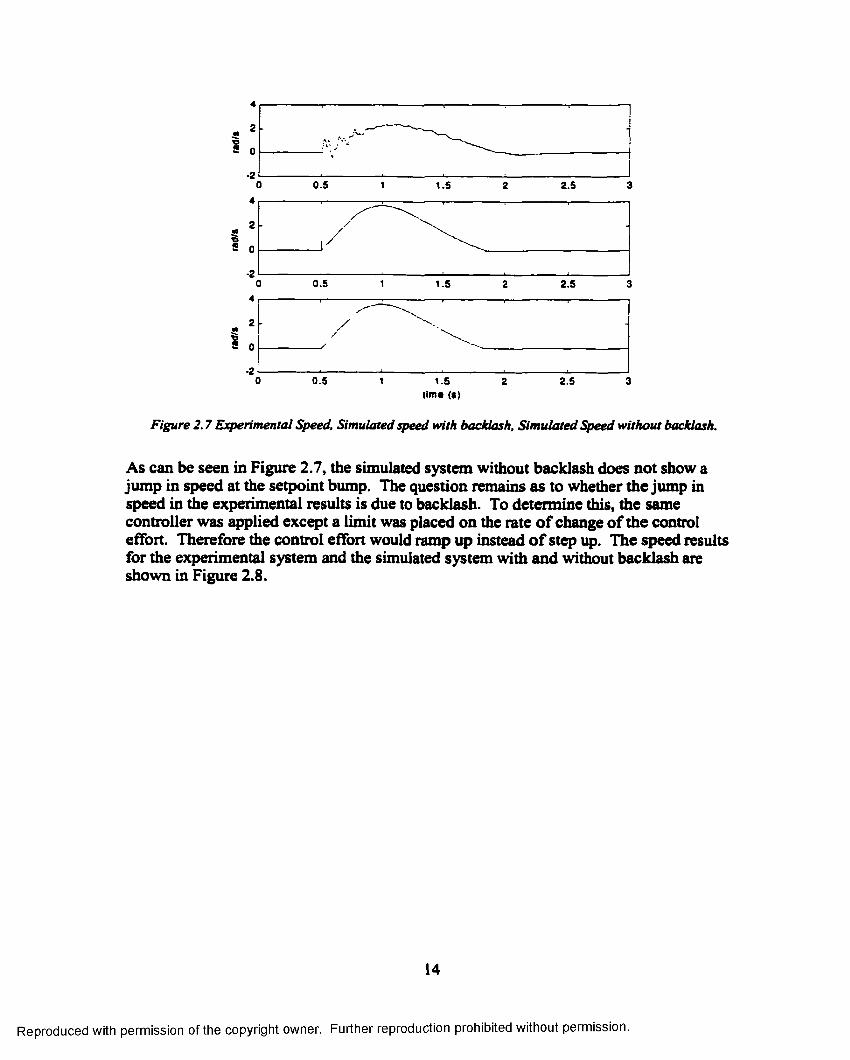
As can be seen in Figure 2.7, the simulated system without backlash does not show a jump in speed at the setpoint bump. The question remains as to whether the jump in speed in the experimental results is due to backlash. To determine this, the same controller was applied except a limit was placed on the rate o f change o f the control effort. Therefore the control effort would ramp up instead o f step up. The speed results for the experimental system and the simulated system with and without backlash are shown in Figure 2.8.

14


titn* (a)

Figure 2.8 Experimental Speed, Simulated speed with backlash. Simulated speed without backlash.Controller rate has been constrained.

The experimental system no longer shows a huge jum p in speed. Oscillations are still present in the speed, however. For the simulated system with backlash a junq) in speed is still visible although it is smaller. The simulated system never shows oscillations in the speed. Additionally, were the jump in speed in the experimental system o f Figure 2.7 (controller not constrained) due to backlash, the system would also show a jump in speed when the speed crossed the zero axis (i.e. the arm changed direction) at about 2 s; however it does not. Therefore we can conclude that backlash has little discernible effect on this system. This is likely due to the fact that the backlash is small (less than one degree) and the friction in the system is quite large.

2.4 Effects of Flexing on Speed

Figure 2.9 is a plot of the experimental results from Figure 2.6 and shows the speed, the base gage reading and the second gage reading. It can be seen that the oscillatory behaviour in the speed is a delayed version o f the oscillatory behaviour exhibited by the second gage. This is significant because the second strain gage monitors beam flexing; therefore the flexing o f the beam is affecting the motor speed. The shape o f the base gage measurement exhibits the oscillatory behaviour o f the second gage measurement, and additionally, has a strong resemblance to the control effort (this is also shown in Figure 4.20 and Figure 4.21). This is expected since both the beam flexing and the control torque will put strain on the beam at the hub.

15


I"

10

I 5

*Î.ri:

- ■

0 0.5 1 1.5 2 2.5 3

•••V'

r- --- - ------^

0 0.5 1 1.5 2 2.5 31

-

V - -

D 0.5 1 1.5 2 2.5 3lima (t)

Figure 2.9 Experimental Speed, Base Cage and Second Cage Measurements

The experimental results show that there is coupling between the motion o f the hub and the arm, and the flexing o f the arm and the hub speed, and thereby demonstrate that the flexible arm dynamics have a significant effect on the total system dynamics. The simulation results show that the system behaviour is not accurately modeled when the flexible arm dynamics are not included in the model, although the backlash has been included. Simulation result in Chapter 3 will show that a model that includes the flexible arm dynamics, while omitting backlash, adequately models the system behaviour.

2.5 Conclusions

Simulation of the system, as a rigid body only, demonstrates that the small backlash present has very little effect on the system dynamics. The remaining significant nonlinearities in the system are Coulomb and static friction. Chapter 3 considers the effects o f these nonlinearities on system behaviour.

The next chapter models the flexible behaviour o f the arm and combines the flexible body and rigid body dynamics into one coupled system. Friction is included in the model. However, bacUash is not. The results in the next chapter will reinforce that backlash can be neglected for this system.

16


Chapter 3

System Model Combining Rigid Body and Flexible Arm Dynamics

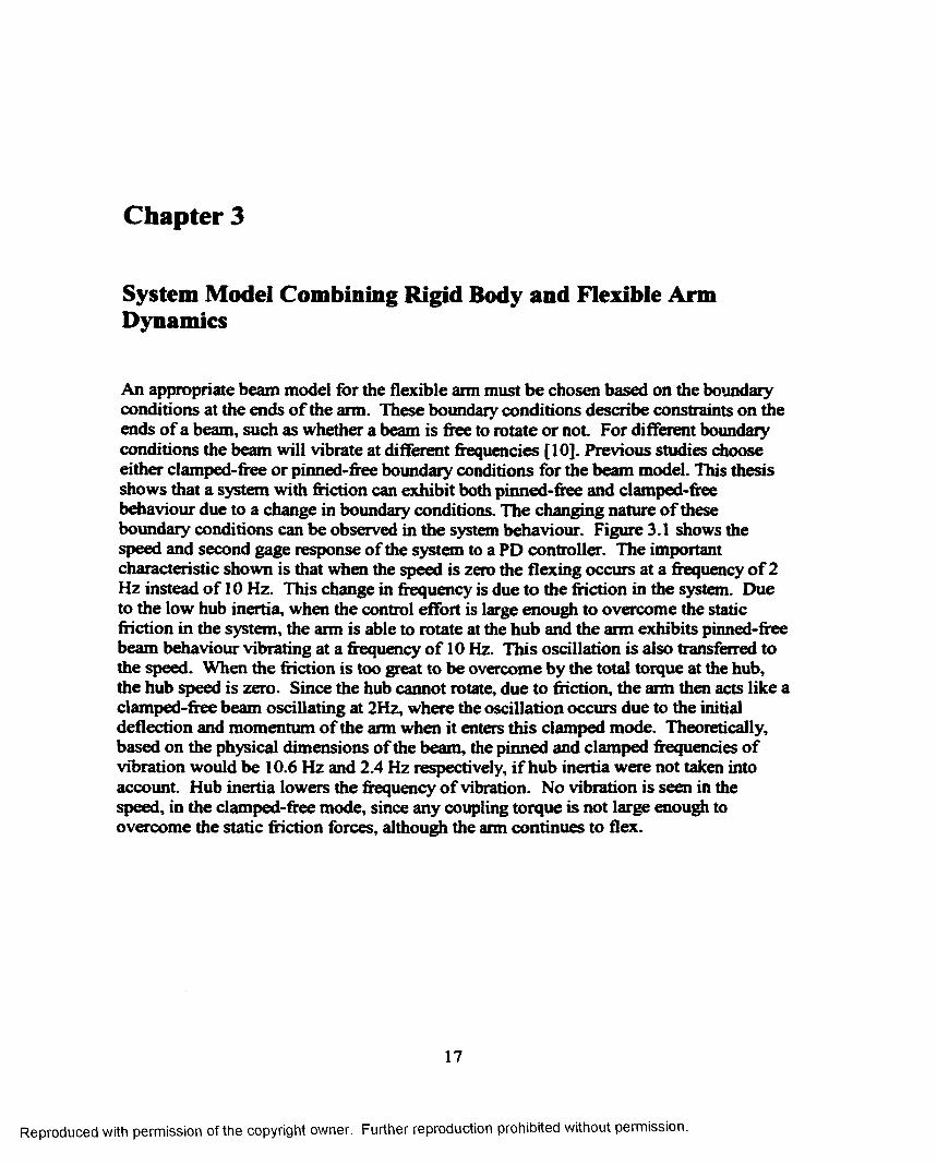
An appropriate beam model for the flexible arm must be chosen based on the boundary conditions at the ends o f the arm. These boundary conditions describe constraints on the ends o f a beam, such as whether a beam is free to rotate or not. For different boundary conditions the beam will vibrate at different frequencies [10]. Previous studies choose either clamped-free or pinned-free boundary conditions for the beam model. This thesis shows that a system with friction can exhibit both piimed-free and clamped-free behaviour due to a change in boundary conditions. The changing nature o f these boundary conditions can be observed in the system behaviour. Figure 3.1 shows the speed and second gage response o f the system to a PD controller. The important characteristic shown is that when the speed is zero the flexing occurs at a frequency o f 2 Hz instead o f 10 Hz. This change in frequency is due to the friction in the system. Due to the low hub inertia, when the control effort is large enough to overcome the static friction in the system, the arm is able to rotate at the hub and the arm exhibits pinned-free beam behaviour vibrating at a frequency o f 10 Hz. This oscillation is also transferred to the speed. When the friction is too great to be overcome by the total torque at the hub, the hub speed is zero. Since the hub cannot rotate, due to friction, the arm then acts like a clamped-free beam oscillating at 2Hz, where the oscillation occurs due to the initial deflection and momentum o f the arm when it enters this clamped mode. Theoretically, based on the physical dimensions o f the beam, the pinned and clamped frequencies o f vibration would be 10.6 Hz and 2.4 Hz respectively, i f hub inertia were not taken into account. Hub inertia lowers the frequency o f vibration. No vibration is seen in the speed, in the clamped-free mode, since any coupling torque is not large enough to overcome the static friction forces, although the arm continues to flex.

17


2.5

1.5

^ 0.5Sa1S(O

-1.5

0 2 2.50.5 3 3.51 1.5 4.5 54tim« (t)

Figure 3.J Experimental Second Gage (V) (green) and Speed (rad/s) (blue) fo r system with no payload

Therefore, two different beam models must be used in modeling the flexible arm portion o f the system — a clamped-free model, and a pinned-free model. The beam models will combine with the rigid body system in different ways — the clamped model will use an explicit coupling term while the pinned model does n o t A combined rigid-flexible body model must be determined for both the pinned and the clamped cases. The boundary conditions o f the simulation will then determine when each model is used.

The flexible body dynamics o f the system refer to the deflection o f the beam from the expected rigid body position. The equations for this motion can be determined using the Lagrange equations and the assumed modes method [19]. If the deflection is assumed to be the sum o f the generalized coordinates multiplied by shape functions, the equations can be determined by computing the generalized mass, generalized stiffness, generalized force, and generalized moment. The generalized coordinates and shape functions can be determined using the finite-element method. This is less labour intensive than solving the Euler-BemouUi beam equation, which is a fourth order partial differential equation [9]. Also, system constants such as hub inertia and payload mass must be included in the boundary conditions when solving the partial differential equation. Thus for any changes in these values the equations must be re-solved before a model can be obtained. In the finite-element method this is not necessary and in the resulting total system such values can be updated directly if they change. This is advantageous when modeling a system with varying payload, especially if the model will be used for real-time control.

18


3.1 Pinned-Free Beam Model

For simplicity, the beam is modeled as a single finite element. This is adequate since the system behaviour is dominated by the first mode, which is a relative simple sluqxe fimction [19]. If a pinned-beam is modeled as a single finite element, there are three generalized (independent) coordinates; slope o f the beam at the hub, 6 i, the tip deflection, vj and the tip slope 6 2 . The deflection of the beam at any point along its length is then:

y(X, t ) = (t)pj (X) + V; ( / ) ^ 2 + 2 ( 0 ^ 3 ( * ) (3.1)

where 0 2 and 0 3 are the shape functions and x is the distance along the beam, âi, and 6 2 are functions o f time only, and 0 i, 0 2 and 0 3 are functions o f space only (distance,x).

M,

Figure 3.2 Beam Deflection in the x-y plane.

The generalized mass, Mb and generalized stiffiiess. Kg, are determined fix>m these shape functions [19]. Knowing these values as well as the generalized forces. A//, M 2 and F^, the equation for the flexible body system is:

A/.' e : ' m ;

2 + ATg =

.^2. M 2 .

(3.2)

The shape functions must be chosen to satisfy the boundary conditions o f the system. For the case o f a pinned-fi’ee beam the boundary conditions are:

y(0,r) = 0 y iL ,t) = \ ’2/(O ,r) = 0, y (Z ,,0 = 2

(3.3)

19


The beam deflection at any time is chosen to be a third-order polynomial in x since this is the lowest order polynomial that can be a solution to the fourth order homogeneous Euler-Bemoulli beam equation. If the beam deflection is chosen as;

y (x ,t) = a^x^ +Û2X^ +û ,x+ûo

Then based on the boundary conditions, the constants are foimd to be;

flo = 0a, =a,

Substituting these constants into Equation (3.4) and rearranging gives;

y (x ,t) = ât(t) ^ 2 x ‘ x M . / - 2x^ 3x2^+ + v,(r) + + 2(0

# 1 * 2

y(x, t) = (r)0 , (x) + V, (t )0 2 (x) + 0 2 (t)A (x)

(3.4)

(3.5)

(3.6)

The generalized mass matrix [19] is given by;

Af a = [m j J where m{x)0 i0 jdx (3.7)

where m(x) is the mass per unit length on the beam (assumed to be constant, i.e. m(x) = m).

The generalized stiffiiess matrix [19] is given by;

- k> J where EI0 ^ jd x (3.8)

where E is the modulus o f elasticity for 6061-T6 Aluminum Alloy and I is the area moment o f inertia o f the arm.

For the pirmed system, the torque at the hub causes the movement o f the arm that leads to a change in 0/ and the subsequent beam vibration. From the rigid body equations in Section 2.1 the torque at hub in terms o f motor gear angle is;

20


The only force acting on the beam is a torque applied at the hub. Therefore,

^1 = - T „ f sgn(0„) ] - ~ “ ( j M2 + J g 2 ) ~ - Sgn(^„)Fj = 0A/, = 0

(3.9)

The moment, Af/, is the equation that links the rigid body to the flexible body. Since the arm angle is related to the motor angle through the gear ratio, the substitution 6i = 0„/N is made in Equation (3.2), and the resulting system has the state variables dm-, vj, and 02,

Therefore, the dynamic equation for the combined rigid-flexible body system is:

M rA ' A A "

2 2 2/2 _ E 2 .

= Qt

where

A/g,, 1 M 2

N ^ B\2

M r = ^ B2\

Afa3i^ B22

Affl23

rK r = K , Q = 0 r = N r , - T f

0

mL' AÜ 131 - 3 Û ^

M — \3L-3 1 }

156- 2 2 1

- 2 2 141:

IT —iW g -420 ^ B

M

MM

A31

A32

A33

Br = 01x2

Ô

Tf = NT„f sgn(^„ ) + sgn(^„ )

ELÜ

AÛ - 6 1 2Û- 6 1 12 - 6 12Û - 6 1 41:

21


These equations are written in state-space format as:

x = Ax+ Buy = Cx (3.10)

where x =

A '^2

^ 2 ^ 2

V2 ^2

Ë 2 .

and u — T — NZg — T f . (3.11)

A —0 : /

Aff'ATr: Mr'Bf (3.12)

B -0

, and C =

l / N 0 0 0 0 00 1 0 0 0 00 0 1 0 0 00 0 0 1 0 00 0 0 0 1 00 0 0 0 0 1

(3.13)

A payload mass acts as a force on the end o f the beam, F«, where . Toinclude a payload in the calculations, only the mass matrix, Mb o f the flexible body equations changes such that:

BPayloatl ^ BNo_mass

0 0 00 ntj 00 0 0

(3.14)

It should be noted that although Equation (3.10) appears linear, due to the dependence o f u on sgn(^„ ) through T/, this equation is nonlinear.

3.2 Clamped-Free Beam Model

For the clamped-free beam modeled as a single finite element, there are only two generalized (independent) coordinates: the tip deflection, vj and the tip slope 02. The

22


deflection o f the beam at any point along its length is then:

y{x,t) = V, (x) + e , (0^2 W (3.15)

where pi and pi are the shape functions and x is the distance along the beam. Note that vj and O2 are functions o f time only, and pi and p2 are functions o f space only.

Figure 3.3 Beam Deflection in the x-y plane.

The generalized mass, Mb and generalized stifhiess, Ks, are determined firom these shape functions. Knowing these values as well as the generalized forces. Mi and F^, the equation for the flexible body system is:

M .A

+ K, * 2

My(3.16)

The shape functions must be chosen to satisfy the boundary conditions o f the system. For the case o f a clamped-free beam the boundary conditions are:

y(0 ,/) = 0 y ( I , / ) = V2y'(0,r) = 0 y \L , t) = Oy

If, as in Section 3.1, the beam deflection at any time is chosen to be a third-order polynomial in x:

y(x ,/) = fl,x^ +ayX^ +ajX+a^

then based on the boundary conditions, the constants evaluate to:

(3.17)

(3.18)

23


a^ = a j = 0_ 3 0y

Û L— . ^2 ~ 1}

Substituting these constants and rearranging gives;

(3.19)

y(x,/) = v,(/) ( - 2 x ^ Zx^ 1Ü 1} + ^ , ( 0

(3.20)

y(x , t) = V , (/)^, (x) + 202

The generalized mass matrix is given by:

M b = WijJ where niy = mix)p^pjdx

The generalized stifrhess matrix is given by:

= k y J where = j^EIp^pjdx

(3.21)

(3.22)

For the combined system, the loading on the clamped beam is caused by the accelerating hub. The acceleration o f the hub, 0^, causes a distributed force on the beam, p(x), whichcan be represented by a force and a moment at the tip o f the beam, F: and Af?. These can be calculated from the generalized force equations:

^ P ix )p (x)dx

Af. = jT pix)p2(x)dx(3.23)

where p{x) = -m 0 ^x is the distributed force on the beam [19,17].

F, = = 2isiL 0_ = F .0 .20

(3.24)20(iV)

(3.25)

24


m û20(A )

Flexible Armhub

Fiffire 3.4. Positive direction o f reaction torque, at the hub caused by flexing o f the arm due to appliedtorque r,.

Figure 3.4 illustrates the positive direction o f the torque acting on the hub {Mo) [16] due to the flexing o f the beam when a torque o f r/ has been applied to the hub. Note that for the deflection shown in Figure 3.4 the value o f Mo will be negative since it opposes the applied torque. The variables T/,û)n, and Mo act on the motor side o f the gears.

The moment at any point along the arm can be found fiiom;

M (x) = E Iy'{x,t)

The equation for the rigid body can now be changed to;

r ,+ M „ = J0 „ ,+ b 6 „ + T f (3.26)

(3.27)

where M„ is the moment on the hub caused by the flexible body referred to the motor side o f the system. The static friction component of 7/must now oppose both Ta and Mo, when the speed is below the static friction threshold.

Combining the flexible and rigid bodies gives the dynamic equation:

M rX ' 'K^2 4-Br ^2 + K r

A . A . X .

= Q t

25


where

0 0 ; J

I ~ A/.

- "0 0 bBt — 0 0 0

- 0 0 0

6EI lE I ; 0 T

^0 e = 0

:o 0

A / , = - mL ■ 156 -2 2 L £7 ' 12 - 6£"420 -2 2 1 4L' ‘ ' T - 6£ 41}

A x+ B u y ~ C x (3.28)

where x =

'*2 V2

^2 ^2, >' =

''2 ^2

A . .

and u — T — x ^ —Tf . (3.29)

sgn(^„ ) + — 7], sgn(^„ )N

M ^'K r(3.30)

B =0

, and C =

l /N 0 0 0 0 00 1 0 0 0 00 0 1 0 0 00 0 0 1 0 00 0 0 0 1 00 0 0 0 0 1

(3.31)

Similar to Section 3.1, if a tip mass is included in the calculations, only the mass matrix, Mb o f the flexible body equations changes such that:

26


^ B P m lo a d ^ B N o ^ m ta sm3 00 0

(3.32)

The rigid body equations change as described in section 2.1.

3 3 Strain Gage Reading Estimation

The second strain gage mounted on the flexible arm gives a measure o f the deflection of the beam referenced to the hub. This strain gage reading can be estimated from the simulated system. The strain on the beam is proportional to the moment on the beam [16]. Therefore, the second strain gage reading is proportional to the moment on the beam at x = 0.55m where the second strain gage is located on the experimental apparatus.

The moment on the beam for the clamped beam is;

M (x) = E Iy'{x,t) = El \2x - 2 6 x \

J)

Therefore, for the clamped model the second strain gage reading can be approximated as;

SG = N ^A /(0.55) = KscEly\(3.55,t) = KscEl{0.6v, +1.3^; ),

where Ksc is a gain introduced by the strain gage circuitry.

In the clamped model and are referenced to the hub, but in the pinned system model they are not, so the strain gage reading for the pinned mode must be approximated by;

SG = K,aM {0.55) = K scEIy\0.55,t) = KscEl{0.6(y, -0^L)+1.3(02 - 0 , ))

By measuring tip deflection and slope for a known strain gage reading Ksc is calculated as 2.27.

3.4 Experimental and Simulated Results

The system is simulated with the same constants used in Section 2.3 and with £ = 68.944 GPa, / = 1.1475e-10 m^, m = 0.42381 kg/m. The system is simulated with a step size o f le-9, using C code, on an SGI Origin 2000 (Cray) and takes approximately twelve hours to run. This long simulation time is due to the small sampling time and the fact that no parallel processing was used.

The systems models are developed for both the pinned and clamped cases separately, and then the models are combined to make one model where the boundary conditions and

27


friction decide what state the model is in. Results are shown for an input current pulse o f 3A, from 0.5 to 1 seconds. At low speeds friction affects system behaviour. Therefore, a large current input was chosen to rotate the arm through a large slew at high speeds, allowing a range o f system behaviour to be seen.

Figure 3.5 and Figure 3.6 show the results for a pinned system with Coulomb friction only. No static friction has been included, since that would theoretically force the system into the clamped mode. Notice that when the speed approaches zero, the Coulomb friction causes the frequency o f vibration o f the system to approach the clamped frrequency. The hub can still rotate and does (however slightly) in this mode as the speed is not yet zero, and therefore, the system is still pinned. The Coulomb friction, which opposes direction o f motion, has a greater effect on system behaviour in this region since as the speed approaches zero it tends to oscillate about zero. Previous studies have mentioned that large hub inertias will cause the pinned frrequency o f vibration to approach the clamped frrequency but this work is the first to note that frriction at low speeds will cause the same effect on a system with small hub inertia.

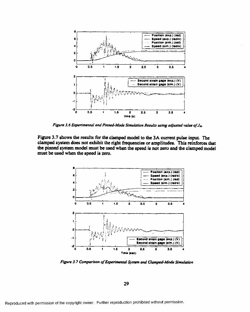
Figure 3.5 shows the system simulation results using the system parameters frrom Table 2.1 in Chapter 2. The frequencies o f vibration for the experimental and simulated case are not an exact match. However, as shown in Figure 3.6, if Jm is adjusted by 0.0003 kgm^ the frrequencies are a better match. This 12% change introduced in the inertia is within the possible experimental error.

Position (oxp.) (rad) Spood (oxp.) (rad/s)— Position (S im .) (rad) Spoad (S im .) (rad/s)

0.5 1.5 2.5 3.5

Second strain gags (oxp.) (V)Second strain gage (sim.) (V)

0.5 1.5 2 2.5time (s)

3.5

Figure 3.5 Experimental and Pinned-Mode Simulation Results using initial calculated value o f

28


Jt

Pod tion (pxp.) (rad) S paad (#%p.) (rad/#)

Position (aim.) (rad) S peed (Sim.) (rad/s)

0.5 1.5 2.5 3.5

Second strain gage (exp.) (V)— Second strain gage (sim.) (V)

‘r t■f

0.5 1.5 2 2.5time (s)

3.5

Figure 3.6 Ejqxrimental and Pinned-Mode Simulation Results using adjusted value o f J„y

Figure 3.7 shows the results for the clamped model to the 3A current pulse input The clamped system does not exhibit the right frequencies or amplitudes. This reinforces that the pinned system model must be used when the speed is not zero and the clamped model must be used when the speed is zero.

f ----- Position (exp.) (rad)----- S peed (exp.) (rad/s) -

Position (sim.) (rad) ----- S peed (S im .) (rad/s) -

i0.5 1.5 2.5 3.5

Socond strain gag# (axp.) (V)Second strain gag# (sim.) (V)

0.5 1.5 2 2.5Tim# (sec)

3.5

Figure 3.7 Comparison o f Experimental System and Clamped-Mode Simulation

29


To accurately model the physical system, the two models must be combined. The simulated system switches between pinned or clamped mode based on the boundary conditions caused by friction. When the speed has remained significantly small for a period o f time, static friction opposes all forces at the hub and the hub wUl no longer rotate. When the hub is not capable o f movement the boundary conditions change and the system switches into clamped mode. Figure 3.8 compares the simulated results for the combined system with the experimental results.

Position (oxp.) (rad) Spaad (axp.) (lad/s) Position (S im .) (rad) Spaad (Sim .) (rad/s)

0.5 1.5 2.5 3.5

I tI ' !4 ,

Second strain g ag e (exp.) (V)- - Second strain gage (sim.) (V)

0.5 1.5 2 2.5 3Time (sec)

3.5

Figure 3.8 Comparison o f combined system simulation and experimental restdts.

Figure 3.9 shows that the smooth oscillations in the physical system can be seen in the simulations if some beam damping is added to the pinned model. This also results in greater amplitude o f vibration, which is closer to the experimental results. However, although there is a physical basis for determining this beam damping, the values o f b and Ttf in Table 2.1 would need to be changed to compensate. Therefore, this damping has not been included in this model. However, the effect on the simulation o f adding damping o f 0.003 Nms to the pinned beam model is shown in Figure 3.9 for interest.

30


Position (oxp.) (rad) Spaad (axp.) (rad/s)

- Position ( S im .) (rad) — Spaad ( S im .) (rad/s)

0.5 1.5 2.5 3.5

Second strain gage (exp.) (V) Second strain gage (sim.) (V)

i0.5 1.5 2 2.5

Time (sec)3.5

Figure 3.9 Effect on the combined system simulation caused by adding beam damping to the pinned model

Position (exp.) (rad)— Speed (exp.) (rad/s)— Position (S im .) (rad) Speed (S im .) (rad/s)

0.5 1.5 2.5 3.5

f.

; 1

Second strain gage (exp.) (V) Second strain gage (sim.) (V)

0.5 1 1.5 2 2.5 3 3.5 4Time (sec)

Figure 3.10 Ejqierimental and simulation results fo r a payload of300g.

Figure 3.10 shows the results o f adding a 300g payload at the end o f the beam. Both simulated and experimental systems show a decrease in the frequency o f oscillation and increase in the amplitude o f the oscillations, which take longer to decay. The advantage o f modeling the flexible beam using the finite element method is that when the payload changes only the value o f m3 must be changed. With the classical methods used in [9] the

31


system equations must be recalculated based on the new boundary condition imposed by the payload.

3.5 Conclusions

The combined flexible/rigid body model predicts the system behaviour more accurately than the rigid body model alone. The rigid body model o f Chapter 2 fails to simulate Üie oscillations in the motor speed, which are due to beam flexing. The flexible body model must be based on the boundary conditions o f the system. While the literature suggests that either a clamped-free or pinned-free beam model can be used, this thesis shows that a system with low hub inertia exhibits both pinned and clamped behaviour due to the friction at the hub therefore the flexible body model must be able to switch between these two models based on the hub speed. When the hub speed is not zero a pinned model must be used, and when the hub speed is zero, due to static friction, a clamped model must be used. For the experimental systems modeled in previous studies [6,7,17] a clamped-free beam model was sufficient since the systems were characterized by high hub inertia or high gear ratio.

Literature has shown that high hub inertia or large gear ratio can cause the pinned mode to asymptotically approach the clamped mode. However, this thesis shows that friction at the hub can cause the pinned frequency o f vibration to ^jproach that o f the clamped mode at low speeds. In this region the hub is still able to rotate, however, and therefore the pinned model must be used. When the hub can no longer rotate due to static friction effects a clamped model must be used.

The finite element model allows for the inclusion o f payload mass as a variable without the need to recalculate the system equations if the payload changes.

Experimental results indicate that hub speed is affected by the flexing of the arm since vibrations in the hub speed are delayed versions o f the vibrations indicated by strain gage readings. Although the clamped model is only appropriate when hub motion is prevented by static fiiction, the clamped model includes a reaction term for the torque on the hub due to beam flexing. This reaction torque can be predicted by the strain gage readings which indicates that strain feedback would be useful in eliminating vibration. Since the pinned model has no explicit reaction term Chapter 4 studies the effect, on the flexible arm vibrations, o f adding the clamped model reaction torque to the control effort.

32


Chapter 4

Controller Design

The model developed in Chapter 3 is a combination o f two separate models that depend on the boundary conditions: a pinned model, and a clamped model. However in terms of behaviour the system can be divided into three separate regions: pinned system under high-speed conditions, pinned system under low-speed conditions, and clamped system. Under low-speed conditions the friction in the system changes the pinned system behaviour, yet the arm can still rotate. When the forces at the hub are no longer able to overcome the friction forces, the system becomes clamped. By simulating the system with different vibration-suppressing controllers it can be shown that the system responds differently to each controller depending on what region it is in.

It has been shown in [11,22,23] that tip acceleration feedback assists in vibration suppression. Strain gage feedback is used in [21] to reduce flexible arm vibration. Previous works have mentioned the intuitive appeal o f using tip acceleration or strain gage feedback for vibration suppression. This diesis uses the strain gage to approximate the coupling torque used in the clamped model developed in Chapter 3. The coupling torque is used to combine the rigid and flexible body equations and suggests that applying a controller to oppose this coupling torque will reduce vibrations at the hub.

Although there are many complex controllers that could be applied to the system model, the vibration-suppressing controller considered here uses signals available for feedback from the experimental system, avoiding the need for an observer, and can be intuitively tuned.

Vibration-suppressing controllers, based on the coupling torque described in Chapter 3, are considered for the two separate models in the three distinct regions o f behaviour, and then for the complete system model. These are discussed in Sections 4.1 - 4.4. In demonstrating the vibration-suppressing controllers no setpoint is used. A current pulse o f 3 A and 0.5 second duration is applied to the motor with the vibration-suppressing controller added directly to this, as in Equation (4.1), as opposed to the traditional negative feedback arrangement, so that the effect o f the vibration-suppressing controller on system behaviour may be observed.

33


2 + ^ jss^ M J L J Æ A f o r0 < t < 0 .5 s

' - ° ' t i ^ z U ) A f o , . > 0 . 5 skijt

The controller is then combined with PD control, based on rigid body hub measurements. In Section 4.5 a comparison is made to PD control alone in response to a setpoint o f 100 degrees.

The results o f the experimental system using vibration-suppressing controllers and PD control are also shown. For the experimental system the control is implemented as shown in Figure 4.1, where the second strain gage is used as an approximation to Mo. In the simulations the calculated value of Mo is used.

Setpont Flexible Manipulator - System

SecondI f f Mo Stwn*\no Estimate

/C|) - Delay K

Figure 4.1 Block diagram o f PD plus vibration suppression control.

/„ = KpCrror — {hub speed) + (4.2)

4.1 Controller Design Based on Clamped Model

In the clamped system model developed in Chq>ter 3, the flexible body is coupled to the rigid body through Mo, given in Equation (3.27), which is repeated here.

£ 7 ^ 6 2 ^M„ =Af(0) = - ^ l — V j ~ — ^ 2 (4.3)

By applying a control effort opposing Mo, it is expected that the effect o f the flexible

34


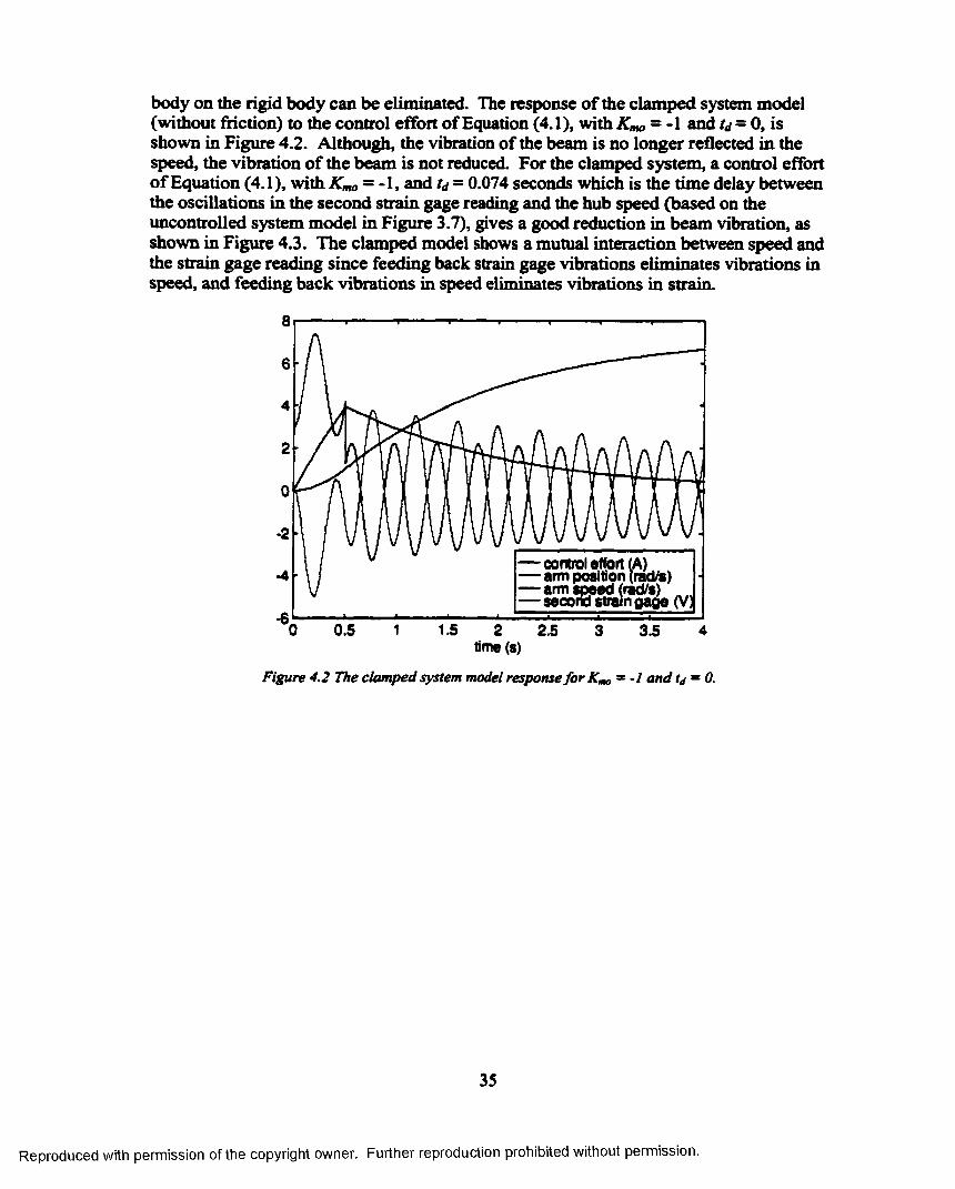
body on the rigid body can be eliminated. The response o f the clamped system model (without friction) to the control effort of Equation (4.1), with Knu> = -1 and td = 0, is shown in Figure 4.2. Although, the vibration of the beam is no longer reflected in the speed, the vibration o f the beam is not reduced. For the clamped system, a control effort o f Equation (4.1), with — -1, and td - 0.074 seconds which is the time delay between the oscillations in the second strain gage reading and the hub speed (based on die uncontrolled system model in Figure 3.7), gives a good reduction in beam vibration, as shown in Figure 4.3. The clamped model shows a mutual interaction between speed and the strain gage reading since feeding back strain gage vibrations eliminates vibrations in speed, and feeding back vibrations in speed eliminates vibrations in strain.

— arm position (rad/fe)— arm sp eed (rad/s)— second sdam g a g e (V |

0.5 1.5 2.5 3.5time(s)

Figure 4.2 The clamped system model response forKmo * -I and tj - 0.

35


roi effort (A) positon (rad/s)— arm positon (rad/s)

— arm sp eed (rad/s)— second strain gage (V)

0.5 1.5 2.5 3.5time (s)

Figure 4.3 The clamped system model response forK^o ~ ~l and tj = 0.074 sec.

The pinned model, which is not explicitly coupled, does not exhibit this behaviour. If a control effort o f Equation (4.1), with Kmo = -1, and td - 0.026 seconds which is the time delay between the oscillations in the second strain gage reading and the hub speed (based on the imcontrolled system model in Figure 3.6), is applied to a pinned system as shown in Figure 4.4, the response is imstable. This indicates that the behaviour o f the pinned and clamped models is different. Therefore, a clamped model will not accurately model a pinned system and a model should be chosen based on the system boundary conations. Figure 4.4 and Figure 4.5 show the simulated results for the pinned system, without and with a current limit of 5 A. Note that for the pinned system the reference for v; and Gj is different and Mo must be calculated using Equation (4.4).

36


— control effort (A)— arm position (rad/s)— arm sp eed (rad/s)— second strain g a g e (V

time (s)

Figure 4.4 The pinned system model (with fiiction) response fo r Kmo = ~J and tj - 0.026 sec.

— control effort (A)— arm position (rad/s)

— — _ j (rad/s) second strain g a g e (V)|

— arm

0.5 1.5 2.5 3.5time (s)

Figure 4.5 Pinned system model response, fo r Kmo ~ -1 and tj = 0.026 sec., with current limited to 5A.

37


10 -

8 ■

6 •

4 ■

2

O-'

-2

-4 •

•6

-8

-10

— control effort (A)— arm position (rad/s) — arm sp eed (rad/s)— second strain g a g e (V

0.5time (8)

Figure 4.6 Experimental system response, fo r Kmo * -I and tj = 0.026 sec., with current limited to 5A.

Figure 4.6 shows the response of the experimental system. It is not surprising that the experimental system is unstable even when the current is limited to SA, since, in Chapter 3. the experimental system showed larger oscillations in the strain gage than the simulated system for the same input and for the experimental system control the second gage reading is used to approximate Mo. When the second strain gage reading is delayed and fed back the controller quickly saturates and continues to oscillate within the saturation limits.

4.2 Controller Design Based on Pinned Model without Friction

Simulation results are shown in Figure 4.7 for the pinned model without Coulomb fiiction. The coupling between the rigid and flexible bodies is not via an explicit coupling term for the piimed system and a reaction torque caimot be determined for this system. However, if a control effort o f Equation (4.1) is applied, with Kmo = -1, and = 0 seconds, and with Mo calculated using Equation (4.4), a reduction o f beam vibration is observed. Mo must be calculated using Equation (4.4) since in the pinned model and 6: are not referenced to the hub.

(4.4)

38


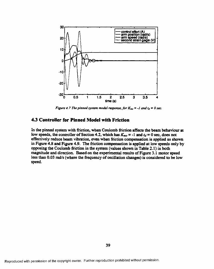
— control effort (A)— arm position (rad/s) — arm sp eed (rad/s)— second strain g a g e (V]

-10

-20

-300.5 1.5 2.5 3.5

tim e(s)

Figure 4.7 The pinned system model response, fo r Kmo ~ -1 and td - Osec.

4.3 Controller for Pinned Model with Friction

In the pinned system with firiction, when Coulomb friction affects the beam behaviour at low speeds, the controller o f Section 4.2, which has Kmo - -1 and r^ = 0 sec, does not effectively reduce beam vibration, even when friction compensation is applied as shown in Figure 4.8 and Figure 4.9. The friction compensation is applied at low speeds only by opposing the Coulomb friction in the system (values shown in Table 2.1) in both magnitude and direction. Based on the experimental results of Figure 3.1 motor speed less than 0.03 rad/s (where the frequency o f oscillation changes) is considered to be low speed.

39


25— control effort (A)— arm position (rad/s) — arm sp eed (rad/s)— second strain g a g e (V;

20

-10

-15

-20

-253.50.5 2.515

tim e(s)

Figure 4.8 The pinned system model (with friction) response, fo r — -I and t j - O sec.

— control effort— arm position — arm sp eed (rad/s)— second strain g a g e (V]|-

1.5 2 2.5time (s)

Figure 4.9 The pinned system mode! (with friction) response, fo r Kmo - -I and = 0 sec. plus low-speedfriction compensation.

The vibration-suppressing controller that is effective in the low-speed region is the controller o f Equation (4.1), with K„o = 1 and ta - 0, plus fiiction compensation. Figure 4.10 shows this controller without fiiction compensation. The controller actually increases the vibrations o f the system until the speed is small where it is effective in suppressing them. Adding fiiction compensation in the low-speed region makes the

40


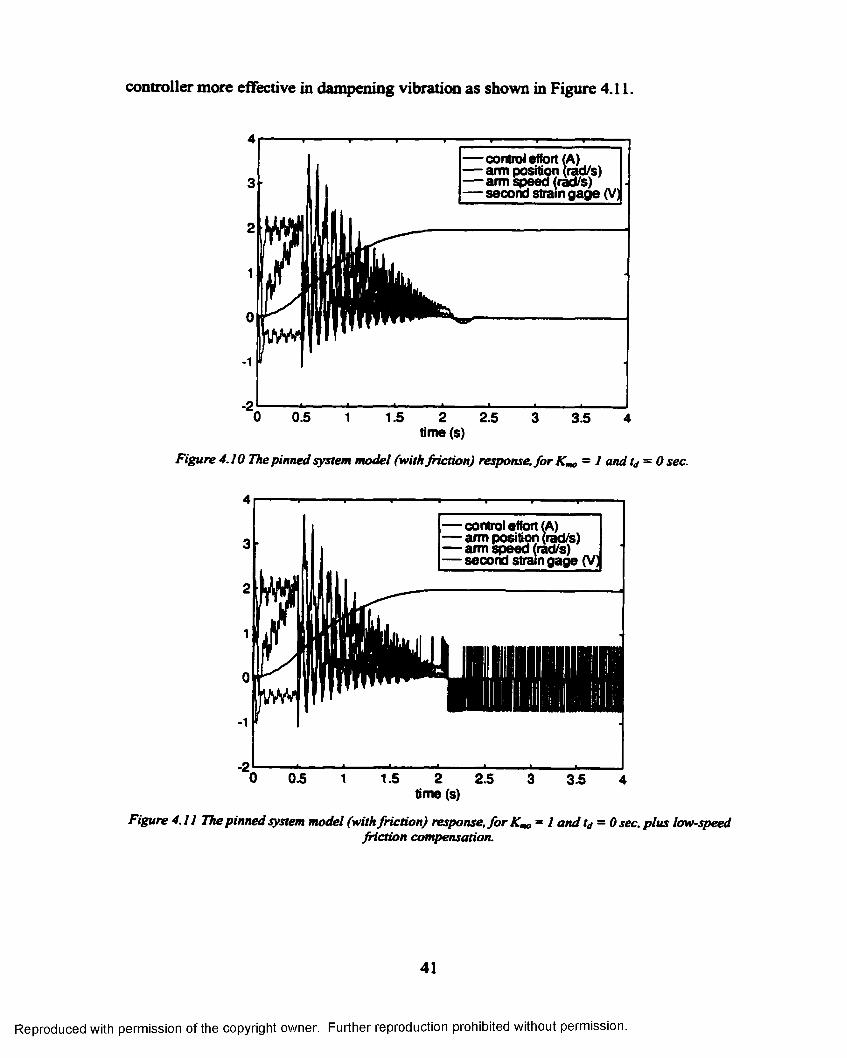
controller more effective in dampening vibration as shown in Figure 4.11.

— control effort (A)(rad/s)— arm position

— arm speed (rad/s)— second strain g a g e (V

tim e(s)

Figure 4.10 The pinned system model (with fiiction) response, fo r = 1 and tj = 0 sec.

— control effort (A)— arm position (rad/s)— arm sp eed (rad/s)— second strain g a g e (V)|

bm efs)

Figure 4. I I The pinned system model (with fiiction) response, fo r K^o = I and = 0 sec. plus low-speedfiiction compensation.

41


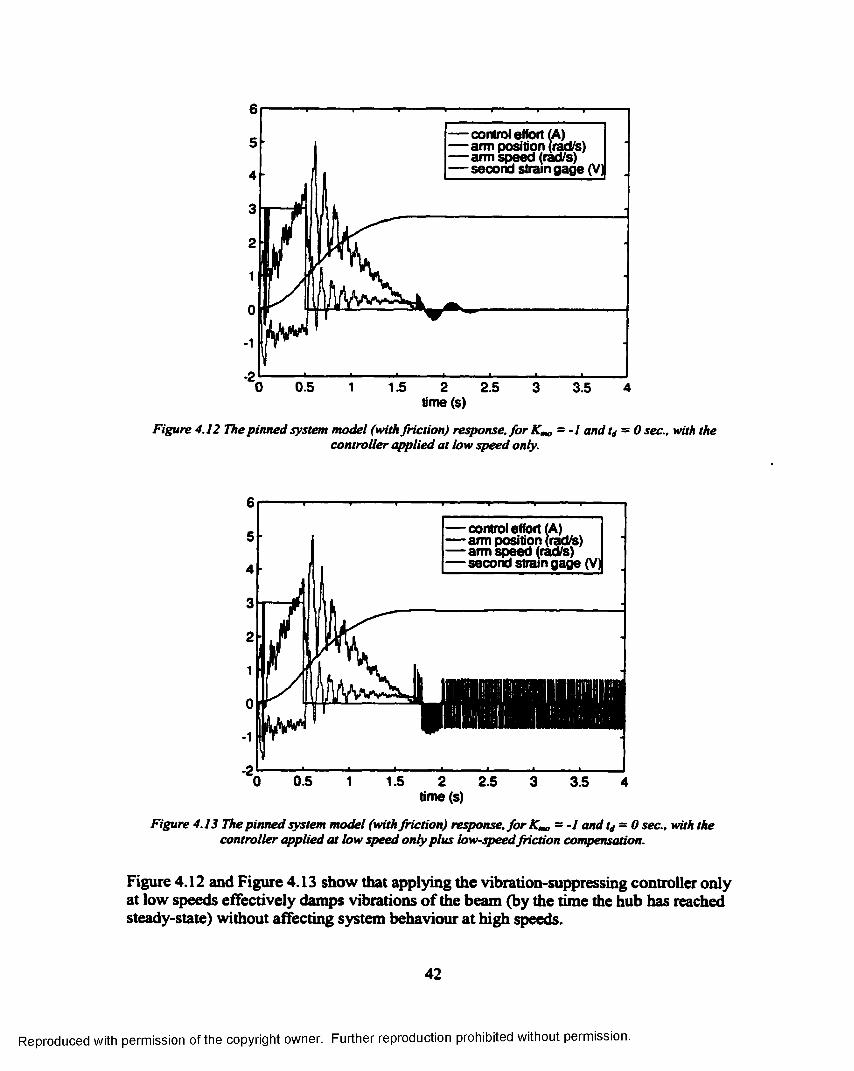
— control effort (A)— arm position (rad/s) — arm sp eed (rad/s)— second strain g a g e (V)

bm e(s)

Figure 4.12 The pinned system model (with fiiction) response, fo r - -I and t j ~ 0 sec., with thecontroller applied at low speed only.

6

— control effort (A)— arm position (rad/s) — arm sp eed (rad/s)— second strain g age (V]

5

4

3

2

1

0

1

■2.0.50 1.5 2 2.5 3 3.51 4

tim e(s)

Figure 4.13 The pinned system model (with fiiction) response, fo r Kmo - -I and tj = 0 sec., with the controller applied at low speed only plus low-speed fiiction compensation.

Figure 4.12 and Figure 4.13 show that s^plying the vibration-suppressing controller only at low speeds effectively damps vibrations o f the beam (by the time the hub has reached steady-state) without affecting system behaviour at high speeds.

42


4.4 Vibration-suppressing Controiler Design for the Complete System

Since the system responds differently to controllers in the pinned, high-speed region (hub speed equal to or greater than 0.03 rad/s), the pinned, low-speed region (hub speed less than 0.03 rad/s) and the clamped region (hub speed equal to zero), the system needs a vibration-suppressing controller that changes depending on the region. The best controller for the pinned region o f system at high speeds is the controller o f Equation (4.1) with K„o — -1 and /</ = 0. For the pinned region o f the system at low speôis the best controller has Kmo ~ 1 and ta - 0 with additional friction compensation. A controller will not be effective in the clamped mode since any control applied in this region will either have no effect ( if it is less than the friction level) or it will force the system into pinned mode where a pinned mode controller would function more effectively. Therefore no controller is suggested for the clamped region. Instead, control should be applied in such a way that when the static friction finally prevents the hub from moving the flexible arm vibrations are already significantly reduced and further control is unnecessary.

Figure 4.14 shows the simulation results for this combined controller. The controller was not constrained to show the system response for the ideal situation o f unlimited control effort.

25— control effort (A)— arm position (rad/s)— arm sp eed (rad/s)— second strain gage (V]

20— arm

-10

-15

-20

-250.5 3.52.5

tim e(s)

Figure 4.14 Complete system model with a combined controller.

4.5 System Response to PD Control with Added Vibration-suppressing Control

It now remains to be seen if this combined vibration-suppressing controller can be an

43


effective addition to a proportional plus velocity feedback controller (PD controller). Figure 4.16 shows the system response for a setpoint o f a 100-degree slew and a controller with PD gains used in Chapter 2 (P=2.5308, D=0.6625) combined with the vibration-suppressing controller while Figure 4.1S shows the response for PD control alone.

— setpoint (rad)— control effort (A)— arm position (rad/s) — arm sp eed (rad/s)— second strain gage (V]

2.5

1.5

0.5

-0.5

-1.5

0.5 2.51.5 3.5tim e(s)

Figure 4.15 System response to a setpoint o f I OOP with PD control.

— setpoint (rad)— control effort (A)— arm position (rad/s)— arm sp eed (rad/s)— secorid strain gage (V]

0 0.5 1

Figure 4.16 System response with PD and combined controller.

44


— arm position (rad/s) — “ rr^ (rad/s)

— second strain g age (V;2.5 — arm

1.5

0.5

-0.5

-1.5

0.5 1.5 2.5 3.5time (s)

Figure 4.17 Total system with PD control and with vibration-suppressing control in the low-speed pinnedregion and clamped region only.

5

4 — arm position (rad/s) — arm sp eed (rad/s)— second strain g a g e (V;3

2

1

0

1

-2

-30.5 1.50 2 2.5 3.51 3 4

time (s)

Figure 4.18 Total System with PD Control and with vibration-suppressing control at high speeds only.

45


0.60.5

0.4

0.3

02a»0.1

- 0.1

— PD Control — PD with -Mo/Mo/_ ContfO

= g g a ......................-0.3 control

.control-0.42 2.51.51 3 3.5 4

time (s)

Figure 4.19 Strain Gage Comparisons.

A comparison o f Figure 4.15 and Figure 4.16 shows that an increase in steady-state hub position error is observed in Figure 4.16. However, by the time the hub position has reached steady-state, the flexible arm vibrations are reduced as compared to Figure 4.15. The system response to PD control with vibration-suppressing control (as per Section 4.4) in the low-speed pinned and clamped regions only is shown in Figure 4.17. From comparison o f Figure 4.15, Figure 4.16 and Figure 4.17, the best results are achieved for vibration suppression control in the low-speed pinned and clamped regions only, added to the PD control. Steady-state hub position error is the same as for PD control alone however flexible arm vibrations at the time the hub speed goes to zero are reduced. Unfortunately, as shown in Figure 4.16, Figure 4.17 and Figure 4.19, when friction compensation is applied at low speeds the system tends to overconqiensate. In a system with noise, this effect is amplified and the overall response is poor. Therefore the most practical controller for suppressing vibration is the vibration-suppressing controller for the high-speed piimed region only (with no vibration-suppressing controller at low speeds), as shown in Figure 4.18, which reduces the oscillations, as much as possible, before static friction prevents the hub rotation.

The experimental results for this controller are shown in Figure 4.21, while Figure 4.20 shows the experimental results for PD control only. The experimental second strain gage reading is used to approximate Mo by multiplying the reading by a gain, K , as shown in Figure 4 .1. Based on comparison o f experimental data with simulated ^ t a a gain o fK - 1.18 was used. The vibration o f the flexible arm when the hub position has reached steady-state is reduced as shown in Figure 4.21, however there is an increase in steady- state hub position error. Figure 4.22 compares the strain gage readings o f Figure 4.20 and Figure 4.21. Additionally, for the experimental system, it is difficult to separate the low-speed pinned region (where the hub can still rotate) from the clamped region (where

46


stade fricdon prevents hub rotadon) due to the noisy speed signal; therefore applying the vibradon-suppressing controller o f Secdon 4.4, for the low-speed regions, would be difficult.

-1

— ««point (rad)— control eflort (A) arm position (rad/s)— arm speed (rad/s)

1 -10 0.5 1 1.5 2 2.5 3 3.5 4 4.5 5

time (s)

(a)

-1

•2

second strain gage (V) base strain gage (V)

0 0.5 1 1.5 2 a s 3 3.5 4 4.5time (s)

(b)Figure 4.20 Experimental System with PD control.

47


setpoint (rad) control effort (A)

ann position (rad/s)— arm spaed (rad/s)

0.5 1.5 2.5 3.5

(a)

2

— second Strain gage (V) base strain gage (V)

0.5 1.5 2.5 3.5time (s)

(b)Figure 4.21 Experiment response fo r a PD control with vibration-suppressing control at high speed.

48


0.8

0.6g

0.4

■0.4

- 0.6 contro

2 2.51.5 3 3.51time (s)

Figure 4.22 Experiment Strain Gage Comparisons.

4.6 Conclusions

The combined model has three main regions o f behaviour—pinned system at high speed, pinned system at low speed and clamped system. Each region responds differently to vibration-suppressing controllers, and theoretically, for maximum effectiveness a different controller should be used in each region. Notably, the controller that effectively suppresses vibration in the clamped-system simulations, is unstable in pinned-system simulations and when applied to the experimental system. Previous studies [21] have noted that a phase shift introduced on strain feedback can make the system unstable.

Friction compensation in the low-speed pinned region tends to overcompensate. The noise in the experimental system would increase these vibrations making the vibration- suppressing control ineffective at low speeds. The most effective vibration suppression controller for the experimental system, therefore, is the vibration-suppressing controller for the high-speed pinned region only, with no vibration-suppressing controller applied at low speeds.

When added to a PD controller the vibration-suppressing controller is effective in reducing the flexible arm vibration by the time the hub position has reached steady-state at a cost o f some steady-state hub position error.

The vibration suppression controller presented in this chapter is advantageous in that it uses available sensor readings and can be intuitively tuned for an experimental system without running simulations. This controller is computationally efficient and inexpensive which makes it easy to implement and maintain.

49


Chapter 5

Conclusions and Future Work

This thesis has produced several new observations on the bdiaviour o f flexible manipulator systems. A flexible manipulator system with friction will exhibit both p in n ^ and clamped frequencies o f vibration. At high speeds, for a system with low hub inertia, the arm is able to rotate and exhibits pinned frequencies. When the speed is zero and static fnction at the hub prevents the arm from rotating, it vibrates at clamped frequencies. Therefore, to model the complete system, a pinned and a clamped model must be used and the boundary condition at the hub must be used to switch between models.

This thesis also demonstrates that at low speeds friction causes the pinned frequencies o f vibration to approach the clamped frequencies. This region differs from the clamped region since die hub is still capable o f small movement. Therefore, a flexible arm system has three different regions of behaviour pinned at high speeds, pinned at low speeds and clamped. In simulation, each o f these regions responds differently to vibration- suppressing controllers, thus requiring a different controller in each region for maximum performance. Vibration suppression controllers based on feedback o f a strain gage reading from the beam are demonstrated for each region through simulation. Practically, while the controller used in the high-speed region provides good vibration suppression, the best control in the low-speed region is no controller due to the noise in the strain gage reading. Experimental and simulation results demonstrate that the final vibration suppression controller design, when added to PD control, reduces arm vibration by the time the hub position reaches steady-state compared to PD control alone.

A non-linear model, which includes friction and is valid for small and large rotation angles, is used to model the system. The small amount o f backlash, due to the gears in the experimental system, has little effect on system bdiaviour and has not been included in the final model. Payload mass can be easily added to the model without the need to recalculate the beam model equations.

Suggestions for future work:

♦ Investigate filtering techniques on strain gage measurements so that feedback in the pinned, low-speed region can be practically iqyplied yet avoid introducing a phase shift which will make die system unstable.

50


♦ Investigate methods of friction compensation such that position control and vibration suppression are improved without a large increase in settling time.

♦ Explore controller design based on an estimation o f payload mass from the fundamental frequency o f the system. It has been shown in [14] that fundamental frequency estimation is possible within a quarter to half cycle o f the period o f die fundamental. Investigate whether the technique o f[14] can be effectively applied to the flexible manipulator system. If this technique were successful it would be an improvement over the estimation times shown in [22,23].

♦ Placing constraints on the rate o f change o f motor current effectively reduced initial beam vibration as shown in Chapter 2. Further investigation is needed to determine the overall effect on system performance o f constraining the rate o f change o f motor current when controllers other than PD controllers are applied.

♦ Investigate improved modeling techniques for determining strain gage dynamics based on flexible arm behaviour.

51


References[1] Atherton, D.P., Nonlinear Control Engineering, ISBN 0-442-30486-2, Van Nostrand Reinhold Co. Ltd., 1982.

[2] Book, W. J., Maizza-Neto, O., and Whitney, D. E., Feedback Control o f Two Beam, Two Joint Systems with Distributed Flexibility. Journal o f Dynamic Systems. Measurement and Control, 1975, pp. 424-431.

[3] Cannon Jr., R. H. and Schmitz, E., Initial Experiments on the End-Point Control o f a Flexible One-Link Robot. International Journal o f Robotics Research, 1984,3(3), pp. 62-75.

[4] Davis, J. H. and Hirschom, R. M., Tracking Control o f a Flexible Robot Link. IEEE Transactions on Automatic Control, 1988,33(3), pp. 238-248.

[5] Feliu, V., Rattan, K. S., Brown Jr., H. B., Modelling and Control o f Single-Link Flexible Arms with Lumped Masses. Journal o f Dynamic Systems, Measurement and Control, 1992,114, pp. 59-69.

[6] Geniele, H., Patel, R. V., and Khorasani, K., Control o f a Flexible-Link Manipulator. Proceedings o f1995 IEEE International Conference on Robotics and Automation, 1995, pp. 1217-1222.

[7] Geniele, H., Patel, R. V., and Khorasani, K., End-Point Control o f a Flexible-Link Manipulator: Theory and Experiments. IEEE Transactions on Control Systems Technology, 1997, 5(6), pp. 556-570.

[8] Hastings, G. G. and Book, W. J., Experiments in Optimal Control o f a Flexible Arm. Proceedings o f the 1985 American Control Conference, 1985, pp. 728-729.

[9] Hastings, G. G. and Book, W. J., Verification of a Linear Dynamic Model for Flexible Robotic Manipulators. Proceedings 1986 IEEE International Conference on Robotics and Automation, 1986, pp. 1024-1029.

[10] Jacobsen, Lydik S., and Ayre, Robert S., Engineering Vibrations, McGraw-Hill Book Company, Inc., 1958.

[11] Kotnik, P. T., Yurkovich, S. and Ozguner, U., Acceleration Feedback Control of a Flexible Manipulator Arm. Journal o f Robotic Systems, 1988,5(3), pp. 181-196.

[12] Krishnan, H. and Vidyasagar, M., Control of Single-Link Flexible Beam Using Hankel-Norm-Based Reduced-Order Model. lEEProc.-Control Theory A ppl, 1998, 145(2), pp. 151-158.

52


[13] Leonard, W., Control o f Electrical Drives, Springer-Verlag, 1985.

[14] Natarajan, K., and Sivakumar, Seshadri, Design o f a fixed-point digital filter for state estimation for UPS applications. Can. J.Elect. & Comp. Eng., 1999,24(4), pp. 155- 161.

[15] Nelder, J. A., and Mead, R.., A Simplex Method for Function Minimization, Computer Journal, vol. 7, pp. 308-313, 1965.

[16] Popov, Egor P., Introduction to mechanics o f solids, Prentice-Hall, Inc., 1968.

[17] Sakawa, S., Matsuno, F., and Fukushima, S., Modeling and Feedback Control o f a Flexible Arm, Journal o f Robotic Systems, 1985,2(4), pp. 453-472.

[18] Taylor, J. H. and Lu, J., Robust Nonlinear Control System Synthesis Method for Electro-Mechanical Pointing System with Flexible Modes. Journal o f Systems Engineering, 1995, 5, pp. 192-204.

[19] Thomson, T. and Dahleh, M.D., Theory o f Vibration with Applications, ISBN 0-13- 651068-X, Prentice-Hall, Inc., 1998.

[20] Wang, D. and Vidyasagar, M., Transfer Functions for a Single Flexible Link. Proceedings 1989 IEEE International Conference on Robotics and Automation, 1989, pp. 1042-1047.

[21] Yu, Sicheng, Control o f a Flexible-Link Manipulator, Masters Thesis, Lakehead University. 1997.

[22] Yurkovich, S., Pacheco, F. E. and Tzes, A. P., On-Line Frequency Domain Information for Control o f a Flexible-Link Robot with Varying Payload. IEEE Transactions on Automatic Control, 1989,34(12), pp. 1300-1304.

[23] Yurkovich, S., Pacheco, F. E., On Controller Tuning for a Flexible-Link Manipulator with Varying Payload. Journal o f Robotic Systems, 1989,6(3), pp. 233-254.

53


Appendix A

Détermination of System Constants

Note: with the exception o f Table A. 1 variables and symbols used in this Appendix are particular to each experiment and are not consistent with the rest o f the thesis.

Experiment 1: Calculating the Motor Constant

Name Plate Data

TYPE: MT30M4-35Serial No: KA 6003Small Electrical Motors Ltd. LondonC-84-44-99CONT. STALL TORQUE: 26 INLB MAX RPM: 4000 Pulse Amps: 52 Volts: 140 INSUL: FTACHO: 9.5V/1000RPM

The objective o f this experiment is to calculate the motor constant k<|>. This was done by measuring Va, la, Ra, and the motor speed, m. Then using the following equations, k0 can be calculated. Ra was measured at several different rotor positions and an average value was taken.

Ra = 1.23 ohms

=kp(o

Experimental Results:

Va(V)

la

(mA)Tacho

(V)CO

(RPM)E(V) Tacho

(rad/s)CO

(rad/s) (Vs/rad)5.431 384.2 1.343 93.7 4.912 14.80 14.71 0.33396.464 397.5 1.630 113.8 5.927 17.97 17.87 0.33177.499 411.4 1.917 133.5 6.944 21.13 20.97 0.33118.488 424.8 2.189 152.5 7.915 24.12 23.95 0.33059.492 429.0 2.461 171.2 8.913 27.12 26.89 0.331510.498 443.4 2.743 190.8 9.899 30.23 29.97 0.330311.503 453.2 3.023 210.3 10.891 33.23 33.03 0.329712.489 466.8 3.298 229.3 11.859 36.35 36.01 0.3293

54


k0 has been found to be approximately 0.33 Vs/rad. This is very close to the value that can be calculated by dividing the Nameplate Data voltage reading by MAX. RPM.

140FA (m R P M *27[/60

= Q35A2Vslrad

The tacho reading in the above table comes from the motor's tachometer. In column 6 it is shown as a value in rad/s, converted using the nameplate data conversion factor o f 9.5 V /1000 RPM. The (o reading in the above table has been measured at the arm shaft. It is necessary to correct for the gear ratio before converting this value to rad/s, since it is the motor speed not the arm speed that we desire to measure. The gear ratio is 1.5 as determined from the number of teeth on the two gears. Therefore the motor turns 1.5 times as fast as the arm.

Experiment 2: Determining the Viscous and Coulomb Friction in the Motor and Shaft (without position potentiometer)

The purpose o f this experiment is to plot — = 6(0 + 7}. As this plot is a straight line, the

numerical values o f b and T f can easily be determined. P is the electrical power to the motor at the armature, which ideally is converted to mechanical power.

Ra = 1.23 ohms

Ra was measured at several different rotor positions and an average value taken. The m referred to in the above equation is the motor speed in (rad/s).

Va(V) Ia(mA) Vtacho(V) Ea(V) P(W ) (0 (rad/s) P/©5.016 375 1.208 4.555 1.708 13.3122 0.12836.000 385 1.493 5.526 2.128 16.4529 0.12937.009 415 1.767 6.499 2.697 19.4723 0.13858.028 424 2.055 7.506 3.183 22.6461 0.14068.997 433 2.323 8.464 3.665 25.5995 0.143210.000 442 2.601 9.456 4.180 28.6630 0.145810.99 453 2.887 10.433 4.726 31.8147 0.1485

12.077 464 3.181 11.506 5.339 35.0546 0.152312.995 477 3.440 12.408 5.919 37.9088 0.156113.011 479 3.445 12.422 5.950 37.9639 0.156713.997 483 3.725 13.403 6.474 41.0495 0.157715.008 492 4.012 14.403 7.086 44.2122 0.1603

55


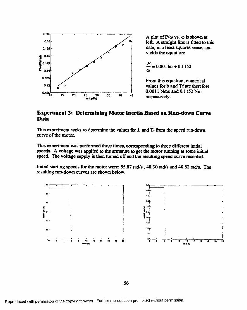
0.165

0.16

0.155

» 0.15

0.135

0.13

0.125.25

A plot o f P/co V S. 00 is shown at left. A straight line is fitted to this data, in a least squares sense, and yields the equation:

— = 0.001 loo+0.115200

From this equation, numerical values for b and T f are therefore 0.0011 Nms and 0.1152 Nm respectively.

Experiment 3: Determining Motor Inertia Based on Run-down Curve Data

This experiment seeks to determine the values for J, and T f ftom the speed run-down curve of the motor.

This experiment was performed three times, corresponding to three different initial speeds. A voltage was applied to the armature to get the motor running at some initial speed. The voltage supply is then turned off and the resulting speed curve recorded.

Initial starting speeds for the motor were: 55.87 rad /s, 48.30 rad/s and 40.82 rad/s. The resulting run-down curves are shown below.

1 .0 -

0 2 4 < • to 12 14 If 20iim# (•)

“ C4S|-

40;- 35 r

— 30 —

i - i. O pJ

2 4 f • 10 12 14 If If 20tint (•)

56


4S|—

40= -

353 0 -

I M-

Î”15-

1 0 -

5

0 10 12 M m # ( • )

The equation for the speed o f the motor based on the system constants with no external torque applied is [13]:

(Û, ( 1)

I f b is assumed to be 0.0011 as previously determined experimentally, we can calculate J and T f using the initial slope o f the curve and the time it takes for the speed to drop to zero.

. By measuring this slope andThe initial slope o f the run-down curve is

knowing ooo and b, J can, theoretically, be determined. To determine T f, the time it takes for the curve to reach 0 rad/s, tc, is determined from the graph. Then with w = 0, b and J known, and tc as determined, T f can be calculated ftom Equation (1). The data for the three experiments is shown in the table below.

coo (rad/s) b(Nms) J(kgm^) tc(s) Tf(Nm) slope(rad/s^) graph of speed55.87 0.0011 0.0006365 0.714 0.02524 -96.5548.30 0.0011 0.0005776 0.625 0.02322 -91.9740.82 0.0011 0.0005212 0.575 0.01898 -86.15

However the value for J seems too small based on the physical size o f this motor. The slope data is somewhat noisy however, so in practice this method is not very good.

If both T f and b are assumed to be the values found in the power balance experiment, and only J is solved for, ftom Equation (1) the following values are obtained.

57


COO (rad/s) b (Nms) J (kgm^) tc(s) Tf(Nm)55.87 0.0011 0.001770 0.714 0.1148.30 0.0011 0.001745 0.625 0.1140.82 0.0011 0.001848 0.575 0.11

These values seem more realistic. For comparison purposes, another method that can be used to find b, J and Tf, is to find the best values for these variables that fit our equation to the rundown curve (from the moment the power is switched off to when the motor stops). This was done using the finins function in Matlab (based on the Nelder Mead technique [15]). The results are shown in the table below. Tfw as assumed to be 0.1192 Nm.

b (Nms) J (kgm“) Tf(Nm) QX) (rad/s)0.00156 0.002032 0.1192 55.870.00136 0.00194 0.1192 48.300.0017 0.002 0.1192 40.82

These values are more consistent with the table above and seem more reliable that just using the initial slope since they use the whole curve.

Experiment 4: Determining the Viscous and Coulomb Friction of the System Including the Flexible Arm.

When the arm is attached to the system, the hub cannot do a full rotation due to physical constraints o f the setup. Therefore, a constant speed cannot be maintained and the previous power experiments cannot be repeated for this case. However, if the speed waveform is periodic in nature then a similar experiment can be performed.

If (Û, is periodic and we integrate both sides o f the equation:

TÛ) - Jûxà+ bû} + Tfû)

With respect to time, over one period, we get:

r / 2 at T / 2 T f l

jro jd t = jjûJd(0+ Jbû?^dt+ jr^axlt- T ' 2 - T U -m

a)

and J J mfù) = 0 thereforeOi

T ' 2 r / 2 r / 2

Jpdt= Jb£0 d/+ ^TfCûdt- r / 2 - r / 2 - r / 2

58

Reproduced with permission o tthe copyright owner. Further reproduction prohibited without permission.

and

r/2 r 2\P d t \Tf<odt7T— = 6 + ^ ------jûJ^dt jû)^dt

- r / 2 - r / 2

which is a straight line with intercept b and slope Tf.

P = EJ„

E a ^ K - I a K

Calculations for the straight-line equation were done for several different data sets, and values o f T f and b were found in each case. These values were then averaged to give T f : 0.188 and b=0.0452, which are the total Coulomb and viscous fiiction respectively.

Experiment 5: Determination of Static Friction

The static fiiction was determined both for the motor and shaft, and for the complete system.

In each case the current to the motor was increased slowly until the speed o f the motor was no longer zero. At this point the current was recorded. By multiplying this current by the motor constant the static fiiction torque is obtained. This experiment was repeated several times and the results averaged. For the motor and shaft only the static fiiction torque was 0.09487 Nm, for the combined system it was 0.2387 Nm.

Calculation o f System Constants

From Experiment 2, the Coulomb fiiction for the motor and shaft was taken as 0.11 Nm, the viscous fiiction was 0.0011 Nms. To isolate the motor fiiction from the shaft fiiction it was assumed that the shaft fnction and motor fiiction were equal. Therefore,

PfcaU PfeotJmotor Pfcouhhaft

where N is the gear ratio. With T&oui = 0.11 Nm then, Tfcouimocor = 0.066 Nm. For the viscous fiiction

^motor

59


With b=0.0011 Nms then bmoior = 0.0008 Nms.

From Experiment 4, the viscous and Coulomb friction for the combined system was taken to be b = 0.0452 Nms and T f = 0.188 Nm. Knowing the friction values for the motor alone, we can solve for the friction values for the arm.

P f 'P fcotdm alor P fam harm

Therefore, T&ouUm, = 0.183 Nm

N 't K

Therefore, b^m = 0.1 Nms

From Experiment 3 the motor inertia was taken as Jm = 0.00193 kgm^. The arm inertia was calculated fit>m the arm dimensions and mass and without payload is 0.15804 kgm^.

With the static friction o f the motor equal to 0.09487 Nm and the total static friction o f the system equal to 0.2387 Nm as determined in experiment 5, the static friction o f the arm is 0.2157 Nm as determined from

T =7*fiu ttia o ta l •* fyuaicm otor •* fiuuicarm

Thus the values used in the simulations are;

System Constant Values used in SimulationJ„ = 0.00193 kgm~ r, / t j = l /N= 1/1.5

- 0.066 Nm (Coulomb) b„ = 0.0008 Nms- 0.09487 Nm (static) bj = 0.1 NmsTgy - 0.183 Nm (Coulomb) m3 = Payload Mass (kg)- 0.21574 Nm (static) ds = I m

= 0.158 + m jd / kgm^ AO = 0.01164

Table A. I System Constant Values used in Simulations

60


2001 Modeling and control of a flexible-link manipulator

Documents

Transcript of 2001 Modeling and control of a flexible-link manipulator