2000-02-14 1 Chinese Cryosphere Information System Li Xin Cold and Arid Regions Environment and...
65
1 2000-02-14 Chinese Cryosphere Information System Li Xin Li Xin Cold and Arid Regions Environment Cold and Arid Regions Environment and Engineering Research and Engineering Research Institute, CAS Institute, CAS
-
Upload
byron-garrett -
Category
Documents
-
view
222 -
download
0
Transcript of 2000-02-14 1 Chinese Cryosphere Information System Li Xin Cold and Arid Regions Environment and...

12000-02-14
Chinese Cryosphere
Information System
Li XinLi Xin
Cold and Arid Regions Environment and Cold and Arid Regions Environment and Engineering Research Institute, CASEngineering Research Institute, CAS

22000-02-14
1. Introduction: Cryosphere and Climate Change 1. Introduction: Cryosphere and Climate Change

32000-02-14
2. Structure of CCIS
data classification andgeo-coding system
system architectureand composition
software and hardwareenvironment
system standard
map projection andscale
data model
databaseimplementation
database
spatial analysis
spatial simulation
application models
application
data exchangeinterface
user interface
systemdemostration
system interface
Ch inese Cryosph eric In fo rm ation System

2000-02-14 4
Hardware and Software Environment in CCIS
ARC/INFO
UNIX Workstation NT Workstation
ArcView
Applications in different environment
PC

52000-02-14
3. Main Case Study Areas of CCIS
Qinghai-Tibet Plateau
Qinghai-Tibet Highway
Urumqi River Basin, Tienshan Mountains

62000-02-14
3.1 CCIS:3.1 CCIS: Qinghai-Tibet PlateauQinghai-Tibet Plateau

72000-02-14
DEMDEM

82000-02-14Map of Frozen GroundMap of Frozen Ground

92000-02-14
Vegetation Map of the QTPVegetation Map of the QTP

102000-02-14
3.2 CCIS:3.2 CCIS: Regions alongRegions along the the Qinghai-Tibet highwayQinghai-Tibet highway
112000-02-14
Database of frozen Soil Engineering Properties along the Qinghai-Tibet Highway

122000-02-14
3.3 CCIS:3.3 CCIS: Urumqi River Urumqi River Basin in the Tienshan Basin in the Tienshan
MountainsMountains

132000-02-14
DEMs of Glacier

2000-02-14 14
4. Spatial Interpolation of Climatic Variables
###
##
#
###
#
#
#
##
#
#### #
#
##
#
#
##
##
# # ##
#
##
##
#
#
#
#
#
#
# # # ##
## # #
## #
##
# #
#
##
# ## ## #
##
#
##
##
#
#
##
##
# # #
#
#
#
#
#
#
#
#
##
#
##
#
##
#
##
#
#
#
#
#
#
#
#
#
#
# #
##
#
#
#
#
#
##
##
#
#
##
# #
# ##
##
##
# ## #
#
##
## ##
##
# ##
105¡ã100¡ã95¡ã90¡ã85¡ã75¡ã 80¡ã
25¡ã
30¡ã
35¡ã
40¡ã
ʨȪºÓ
ÆÕÀ¼
¸ÄÔò
Îé µÀÁº
ÍÐ ÍкÓÂê¶à
¸ñ¶ûľ
ÄÇÇú
ÈÕ¿¦ Ôò ÀÈø
ÄôÀľ
´í ÄÇ
ÓñÊ÷
²ý ¶¼
²ì Óç
Î÷Äþ
ÆøΠ£¨Kriging£©-18--17.6-17.6--16-16--14.5-14.5--12.9-12.9--11.4-11.4--9.8-9.8--8.3-8.3--6.7-6.7--5.2-5.2--3.6-3.6--2.1-2.1--0.5-0.5-11-2.62.6-4.14.1-5.75.7-7.27.2-8
ÆøÏó Õ¾1ÔÂƽ¾ùÆøÎÂ# -18--15# -15--11.9# -11.9--8.9# -8.9--5.8# -5.8--2.8# -2.8-0.3# 0.3-3.4# 3.4-6.4
# 6.4-9.5
# 9.5-12.5
250 0 250 500 750 1000 1250 1500 1750 2000 2250 2500 K ilometersN
Çà²Ø¸ßÔ30Ä꣨1961- 1990£©1ÔÂƽ¾ùÆøΠ·Ö²¼£¨Kr i gi ngÄڲ壩
Missing data estimation
Data gridding

2000-02-14 15
Classification and Procedure of Spatial Interpolation
Geometric method Statistical method Geostatistical method Functional method Stochastic simulation Physical model
simulation Combined method
Data
Model Specification
Estimation of surface mean
Estimation of second order (covariance, variogram)
properties of surface
Model evaluation
Interpolation
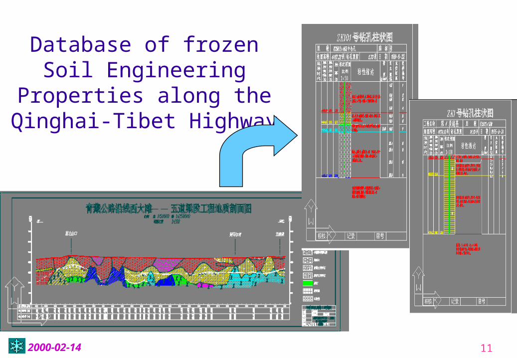
162000-02-14
Meteorological Stations in the Qinghai-Tibet Plateau

2000-02-14 17
Inverse Distance Weighting
n
ip
i
n
iip
i
D
ZD
Z
1
1
)(
1
)(
1

182000-02-14
## ###
#
###
#
#
#
##
#
#### #
#
##
#
#
##
# ## # ##
#
##
##
#
#
#
#
#
#
# # # ##
## # #
## #
##
# #
#
##
# ## ## #
##
#
##
##
#
#
##
## # # #
#
#
#
#
#
#
#
#
##
#
##
#
##
#
##
#
#
#
#
#
#
#
#
#
#
# #
##
#
#
#
#
#
##
# #
#
#
##
# #
# ##
##
##
# ## #
#
##
## ##
##
# ##
105¡ã100¡ã95¡ã90¡ã85¡ã75¡ã 80¡ã
25¡ã
30¡ã
35¡ã
40¡ã
Shiquanhe
Burang
Gerze
Wudaoliang
TutuheMadoi
Golmud
Nagqu
Xigaze Lhasa
NyalamCona
Yushu
Qamdo
Zayu
Xining
Pishan
air temperature (IDW )-17.6 - -16-16 - -14.5-14.5 - -12.9-12.9 - -11.4-11.4 - -9.8-9.8 - -8.3-8.3 - -6.7-6.7 - -5.2-5.2 - -3.6-3.6 - -2.1-2.1 - -0.5-0.5 - 11 - 2.62.6 - 4.14.1 - 5.75.7 - 7.2
air temperature at meteorological stations
# -18 - -15# -15 - -11.9# -11.9 - -8.9# -8.9 - -5.8# -5.8 - -2.8
# -2.8 - 0.3
# 0.3 - 3.4
# 3.4 - 6.4
# 6.4 - 9.5
# 9.5 - 12.5
Interpolation results of inverse distance square

2000-02-14 19
Trend Surface
eAy
qn
pnnnnnnn
qp
qp
aaaaaaaa
aaaaaaaa
aaaaaaaa
A
21212
22
121
222122212
222
212221
121112112
122
111211
1
1
......1
).......( 110220011000 pqT

202000-02-14
## ###
#
###
#
#
#
##
#
#### #
#
##
#
#
##
# ## # ##
#
##
##
#
#
#
#
#
#
# # # ##
## # #
## #
##
# #
#
##
# ## ## #
##
#
##
##
#
#
##
## # ##
#
#
#
#
#
#
#
#
###
##
#
##
#
##
#
#
#
#
#
#
#
#
#
#
# #
###
#
#
#
#
##
# #
#
#
##
# #
# ##
##
##
# ## #
#
##
## ##
##
# ##
105¡ã100¡ã95¡ã90¡ã85¡ã75¡ã 80¡ã
25¡ã
30¡ã
35¡ã
40¡ã
Shiquanhe
Burang
Gerze
Wudaoliang
TutuheMadoi
Golmud
Nagqu
Xigaze Lhasa
NyalamCona
Yushu
Qamdo
Zayu
Xining
Pishanair temperature (trend surface)
-18 - -17.6-17.6 - -16-16 - -14.5-14.5 - -12.9-12.9 - -11.4-11.4 - -9.8-9.8 - -8.3-8.3 - -6.7-6.7 - -5.2-5.2 - -3.6-3.6 - -2.1-2.1 - -0.5-0.5 - 11 - 2.62.6 - 4.14.1 - 5.75.7 - 7.27.2 - 8
air temperature at meteorological stations
# -18 - -15# -15 - -11.9# -11.9 - -8.9# -8.9 - -5.8# -5.8 - -2.8
# -2.8 - 0.3
# 0.3 - 3.4
# 3.4 - 6.4
# 6.4 - 9.5
# 9.5 - 12.5
Interpolation results of trend surface

2000-02-14 21
Kriging methodKriging method
n
iii xzxz
10 )()(
n
ii
1
1
n
iiie xx
10
2 ),(
jxxxx j
n
ijii
),(),( 01

2000-02-14 22
Exploratory Spatial Data AnalysisExploratory Spatial Data Analysis The mathematical expectation of the difference
between two points separated by distance h is zero:
0)]()([( hxZxZE The variance of the difference between two points
separated by distance h is minimized as:
Hence, the semi-variance can be calculated from data samples by the following equation:
)(2]})()({[)]()([ 2'' hxxEhxZxZVar
2
1
])()([2
1)(
n
iii hxzxz
nh

2000-02-14 23
Basic variogram models
0 h
(h)
0 h
(h)
0 h
(h)
0 h
(h)
0 h
(h)
0 h
(h)
Nugget model Spherical model Exponential model
Gaussian model Holesin model Linear model

2000-02-14 24
Cokriging methodCokriging method
cokriging introduces a new hypothesis, the variance of the
difference between two variables is minimized
The equation of cross-variogram is as follows:
)(2)]()([ hxZxZVar kk
)]()(][)()([2
1)(
1
hxzxzhxzxzn
h ik
ik
n
iii
k

252000-02-14
Fit of simple and cross-variogram

262000-02-14
## ###
#
###
#
#
#
##
#
#### #
#
##
#
#
##
# ## # ##
#
##
##
#
#
#
#
#
#
# # # ##
## # #
## #
##
# #
#
##
# #### #
##
#
##
##
#
#
##
## # ##
#
#
#
#
#
#
#
#
###
##
#
##
#
##
#
#
#
#
#
#
#
#
#
#
# #
###
#
#
#
#
##
# #
#
#
##
# #
# ##
##
##
# ## #
#
##
## ##
##
# ##
105¡ã100¡ã95¡ã90¡ã85¡ã75¡ã 80¡ã
25¡ã
30¡ã
35¡ã
40¡ã
Shiquanhe
Burang
Gerze
Wudaoliang
TutuheMadoi
Golmud
Nagqu
Xigaze Lhasa
NyalamCona
Yushu
Qamdo
Zayu
Xining
Pishan
air temperature (cokriging)-18 - -17.6-17.6 - -16-16 - -14.5-14.5 - -12.9-12.9 - -11.4-11.4 - -9.8-9.8 - -8.3-8.3 - -6.7-6.7 - -5.2-5.2 - -3.6-3.6 - -2.1-2.1 - -0.5-0.5 - 11 - 2.62.6 - 4.14.1 - 5.75.7 - 7.27.2 - 8
air temperature at meteorological stations
# -18 - -15# -15 - -11.9# -11.9 - -8.9# -8.9 - -5.8# -5.8 - -2.8
# -2.8 - 0.3
# 0.3 - 3.4
# 3.4 - 6.4
# 6.4 - 9.5
# 9.5 - 12.5
Interpolation results of cokriging

2000-02-14 27
Combined methodCombined method Assuming that spatial variable consists of three
components: one structural component, one
stochastic and spatial correlated component, and
one stochastic noise or residual. Let x denotes a
two-dimensional or three-dimensional vector,
spatial variable Z(x) can be expressed as:
'')(')()( xxmxZ

282000-02-14
Lapse rates of different latitudinal and Lapse rates of different latitudinal and altitudinal zones in the altitudinal zones in the
Qinghai-Tibet Plateau (Qinghai-Tibet Plateau (C/100m)C/100m)
表 4-1 青藏高原气温垂直梯度(℃/100米)
海拔(米) 北 纬
1500-2000 2000-2500 2500-3000 3000-3500 3500-4000 4000-4500 4500-5000 平 均
28° 0. 52 0. 52 0. 52 0. 52 0. 54 0. 52 0. 52 0. 52
30° 0. 48 0. 50 0. 48 0. 50 0. 48 0. 50 0. 50 0. 49
32° 0. 54 0. 52 0. 54 0. 54 0. 54 0. 54 0. 54 0. 54
34° 0. 46 0. 44 0. 46 0. 46 0. 46 0. 46 0. 46 0. 46
36° 0. 48 0. 46 0. 48 0. 46 0. 48 0. 48 0. 46 0. 47
平 均 0. 50 0. 49 0. 50 0. 50 0. 50 0. 50 0. 50 0. 50

292000-02-14
## ###
#
###
#
#
#
##
#
#### #
#
##
#
#
##
# ## # ##
#
##
##
#
#
#
#
#
#
# # # ##
## # #
## #
##
# #
#
##
# ## ## #
##
#
##
##
#
#
##
## # # #
#
#
#
#
#
#
#
#
##
#
##
#
##
#
##
#
#
#
#
#
#
#
#
#
#
# #
##
#
#
#
#
#
##
# #
#
#
##
# #
# ##
##
##
# ## #
#
##
## ##
##
# ##
105¡ã100¡ã95¡ã90¡ã85¡ã75¡ã 80¡ã
25¡ã
30¡ã
35¡ã
40¡ã
ʨȪºÓ
ÆÕÀ¼
¸ÄÔò
Îé µÀÁº
ÍÐÍкÓÂê¶à
¸ñ¶ûľ
ÄÇÇú
ÈÕ¿¦ Ôò ÀÈø
ÄôÀľ´í ÄÇ
ÓñÊ÷
²ý ¶¼
²ì Óç
Î÷Äþ
ÆøΠ£¨3000Ã×£©-17.6--16-16--14.5-14.5--12.9-12.9--11.4-11.4--9.8-9.8--8.3-8.3--6.7-6.7--5.2-5.2--3.6-3.6--2.1-2.1--0.5-0.5-1
ÆøÏó Õ¾1ÔÂƽ¾ùÆøÎÂ# -18--15# -15--11.9# -11.9--8.9# -8.9--5.8# -5.8--2.8# -2.8-0.3# 0.3-3.4# 3.4-6.4
# 6.4-9.5
# 9.5-12.5
250 0 250 500 750 1000 1250 1500 1750 2000 2250 2500 K ilometersN
Çà²Ø¸ßÔ30Ä꣨1961- 1990£©1ÔÂƽ¾ùÆøΠ·Ö²¼£¨3000Ã×̧߶ȣ©

302000-02-14
a sum of nugget, linear and Gaussian variogram models

312000-02-14
## ###
#
###
#
#
#
##
#
#### #
#
##
#
#
##
# ## # ##
#
##
##
#
#
#
#
#
#
# # # ##
## # #
## #
##
# #
#
##
# ## ## #
##
#
##
##
#
#
##
## # # #
#
#
#
#
#
#
#
#
##
#
##
#
##
#
##
#
#
#
#
#
#
#
#
#
#
# #
##
#
#
#
#
#
##
# #
#
#
##
# #
# ##
##
##
# ## #
#
##
## ##
##
# ##
105¡ã100¡ã95¡ã90¡ã85¡ã75¡ã 80¡ã
25¡ã
30¡ã
35¡ã
40¡ã
ʨȪºÓ
ÆÕÀ¼
¸ÄÔò
Îé µÀÁº
ÍÐÍкÓÂê¶à
¸ñ¶ûľ
ÄÇÇú
ÈÕ¿¦ Ôò ÀÈø
ÄôÀľ´í ÄÇ
ÓñÊ÷
²ý ¶¼
²ì Óç
Î÷Äþ
ÆøΠ£¨×ÛºÏ £©-25.4--22.5-22.5--20-20--17.6-17.6--16-16--14.5-14.5--12.9-12.9--11.4-11.4--9.8-9.8--8.3-8.3--6.7-6.7--5.2-5.2--3.6-3.6--2.1-2.1--0.5-0.5-11-2.62.6-4.14.1-5.75.7-7.27.2-8
ÆøÏó Õ¾1ÔÂƽ¾ùÆøÎÂ# -18--15# -15--11.9# -11.9--8.9# -8.9--5.8# -5.8--2.8# -2.8-0.3
# 0.3-3.4
# 3.4-6.4
# 6.4-9.5
# 9.5-12.5
250 0 250 500 750 1000 1250 1500 1750 2000 2250 2500 K ilometersN
Çà²Ø¸ßÔ30Ä꣨1961- 1990£©1ÔÂƽ¾ùÆøΠ·Ö²¼£¨×ÛºÏ ·½·¨ Äڲ壩

322000-02-14
## ####
# ##
#
#### #
#### ##
# #
##
## # ## # ##
######
###
#
## # # ## ## # ### # ##
# ##
### #### ###
### ##
#
### ## # ##
##
#
#
#
##
#
###
## #
##
#
# #
#
#
#
#
## #
##
###
## #
#
###
##
# #
##
##
# ## #
#
##
##
# ## #
#
##
## ##
##
# ##
40¡ã
35¡ã
30¡ã
25¡ã
80¡ã75¡ã 85¡ã 90¡ã 95¡ã 100¡ã 105¡ã
## ####
# ##
#
#### #
#### ##
# #
##
## # ## # ##
######
###
#
## # # ## ### #
## # ### #
#### #### #
##
### ##
#
### ## # ##
# ##
#
#
##
#
###
## #
##
#
# #
#
#
#
#
## #
##
###
## #
#
###
##
# #
##
##
# ## #
#
##
##
# ## #
#
##
## ##
##
# ##
40¡ã
35¡ã
30¡ã
25¡ã
80¡ã75¡ã 85¡ã 90¡ã 95¡ã 100¡ã 105¡ã
·½²î0. 22 - 1. 941. 94 - 3. 663. 66 - 5. 385. 38 - 7. 17. 1 - 8. 828. 82 - 10. 5410. 54 - 12. 2612. 26 - 13. 9813. 98 - 15. 71
500 0 500 1000 1500 2000 2500 3000 Kilometers
Cokr i gi ngºÍ ×ÛºÏ ·½·¨ ÄÚ²å ·½²î ±È½Ï
N

2000-02-14 33
ConclusionConclusion Spatial interpolation is a very important spatial analysis tool
in GIS. As for the cryospheric regions with sparsely and irrationally distributed meteorological stations, spatial interpolation is a basic method for the study of spatial distribution of climatic variables and also a prerequisite for the establishment of cryospheric models based on GIS.
There is no absolutely optimal spatial interpolation method; there is only relatively optimal interpolation method in special situation. Hence, the best spatial interpolation method should be selected in accordance with the qualitative analysis of the data, exploratory spatial data analysis and repeated experiments.

342000-02-14
5. Response of Permafrost to Global 5. Response of Permafrost to Global
Change on the Qinghai-Tibet Plateau Change on the Qinghai-Tibet Plateau
- A GIS Aided Model- A GIS Aided Model

2000-02-14
Permafrost Response to Climate Change
Permafrost Forecast
Physical ModelFrost Number Model
Altitude Model
Permafrost Map
GCM Model
Climate Change Scenarios
Geocode l ongi tude Lati tude Ai r Temperatureof WarmestMonth
Ai r Temperatureof Col destMonth
180 100. 65 35. 27 11. 65 -13. 22181 101. 98 35. 90 19. 21 -6. 22182 101. 47 35. 03 8. 71 -14. 63183 102. 45 35. 82 19. 86 -5. 34184 102. 08 35. 50 16. 03 -7. 96185 104. 08 35. 85 18. 93 -7. 95186 103. 18 35. 58 17. 96 -6. 92187 103. 87 35. 37 18. 47 -7. 36188 105. 15 35. 63 18. 14 -6. 95189 104. 60 35. 50 18. 28 -7. 77190 105. 00 35. 38 14. 70 -8. 80191 80. 08 32. 50 13. 51 -12. 29192 84. 42 32. 15 11. 52 -13. 23193 90. 02 31. 37 8. 52 -11. 03194 91. 10 32. 35 7. 66 -14. 73
GIS

2000-02-14
H 3650 0 003 2537 14282exp[ . ( . ) ]
Ph H
h H
1
0
,
,
Altitude Altitude ModelModel

2000-02-14
Geo thermal Regime
GCM Scenarios
Data Flow in the Altitude Model

2000-02-14
DEM of Qinghai-Tibet PlateauDEM of Qinghai-Tibet Plateau

392000-02-14
Diagram of HADCM2Diagram of HADCM2

402000-02-14
# #
#
#
#
##
# #
#
#
#
40¡ã
35¡ã
30¡ã
25¡ã
80¡ã75¡ã 85¡ã 90¡ã 95¡ã 100¡ã 105¡ã
Î÷Äþ
²ý ¶¼
ÓñÊ÷
´í ÄÇ
ÄôÀľ
ÀÈøÈÕ¿¦ Ôò
ÄÇÇú
¸ñ¶ûľ
ÍÐÍкÓ
Îé µÀÁº
ʨȪºÓ ÆøΠÉý¸ß·ù ¶È0.17-0.480.48-0.800.80-1.111.11-1.421.42-1.741.74-2.052.05-2.362.36-2.682.68-2.99
500 0 500 1000 1500 2000 2500 K ilometers
N
2049ÄêÇà²Ø¸ßÔÆøΠÉý¸ß·ù ¶È
The Air Temperature Rise on the The Air Temperature Rise on the Qinghai-Tibet Plateau in 2049Qinghai-Tibet Plateau in 2049

412000-02-14
# #
#
#
#
#
#
40¡ã
35¡ã
30¡ã
25¡ã
80¡ã75¡ã 85¡ã 90¡ã 95¡ã 100¡ã 105¡ã
Golmu
Shiquanhe
Lasa
Cuona
Yushu
Changdu
Xining
Selingcuo Lake
Namuchu Lake
Qinghai Lake
legendPermafrostSeasonalFrozenGroundGlacierDesertLake
500 0 500 1000 1500 2000 2500 Kilometers
N
SimulationResultoftheAltitueModel

2000-02-14
FDDF
DDF DDT
Nelson Frost Number ModelNelson Frost Number Model

432000-02-14
# #
#
#
#
#
#
40¡ã
35¡ã
30¡ã
25¡ã
80¡ã75¡ã 85¡ã 90¡ã 95¡ã 100¡ã 105¡ã
Golmu
Shiquanhe
Lasa
Cuona
Yushu
Changdu
Xining
Selingcuo Lake
Namuchu Lake
Qinghai Lake
Legendcontinouspermafrostdiscontinouspermafrostseasonalfrozengroundglacierdesertlake
500 0 500 1000 1500 2000 2500 Kilometers
N
EW
S
Permafrost Distribution on the Qinghai-Xizang PLateau(Using the Frost Number Model)

2000-02-14 44
Assumptions:Assumptions: The Gaussian function that describes high altitude
permafrost distribution will not change according to the climate warming.
If air temperature increases 1C, the vertical zonation will rise a certain height agreeing on the lapse rate, the lower limit of the high-altitude permafrost will rise the same height. Therefore, a relation can be established between the air temperature rise (ΔT) and the increased height of permafrost lower limit (ΔH). The relation is:
T
H
Lakes, glaciers, deserts will not change

452000-02-14
40¡ã
35¡ã
30¡ã
25¡ã
80¡ã75¡ã 85¡ã 90¡ã 95¡ã 100¡ã 105¡ã
# #
#
#
#
#
#
Golmu
Shiquanhe
Lasa
Cuona
Yushu
Changdu
Xining
Se lingc uo LakeNamucuo Lake
Qinghai Lake
40¡ã
35¡ã
30¡ã
25¡ã
80¡ã75¡ã 85¡ã 90¡ã 95¡ã 100¡ã 105¡ã
500 0 500 1000 1500 2000 Kilometers
LegendPermafrostSeasonalFrozenGroundGlacierDesertLake
N
40¡ã
35¡ã
30¡ã
25¡ã
80¡ã75¡ã 85¡ã 90¡ã 95¡ã 100¡ã 105¡ã
Present Permafrost Distribution
40¡ã
35¡ã
30¡ã
25¡ã
80¡ã75¡ã 85¡ã 90¡ã 95¡ã 100¡ã 105¡ã40¡ã
35¡ã
30¡ã
25¡ã
80¡ã75¡ã 85¡ã 90¡ã 95¡ã 100¡ã 105¡ã
40¡ã
35¡ã
30¡ã
25¡ã
80¡ã75¡ã 85¡ã 90¡ã 95¡ã 100¡ã 105¡ã
Permafrost Change when Air Temperature Rise 0.51°C
Permafrost Change when Air Temperature Rise 1.10°C
Permafrost Change when Air Temperature Rise 2.91°C

462000-02-14
1190
1056
541
1294
0.00
0.51
1.10
2.91
0
200
400
600
800
1000
1200
1400
1990 2009 2049 2099
0.00
0.50
1.00
1.50
2.00
2.50
3.00
3.50Permafrost Area
Air Temperature Rise
Permafrost Change on the Qinghai-Tibet Permafrost Change on the Qinghai-Tibet PlateauPlateau
8.03
18.45
58.18

4799-11-20
6. Other Models6. Other Models

482000-02-14
6.1 6.1 Solar Radiation Model over Rugged TerrainSolar Radiation Model over Rugged Terrain
Duration of possible sunshine Ω: defined as the set of duration when the sloping grid can receive direct solar radiation during the entire day.
Isotropic view factor Viso: defined as the ratio of the area of the visi
ble part to the area of semi-sphere on a sloping grid. It stands for the influence of the surrounding terrain to the isotopic diffuse radiation.
Circum-solar view factor V1: defined as the ratio of the exoatmosph
eric radiance obstructed by surrounding and self-shadowing to the exoatmospheric radiance obstructed only by self-shadowing. It stands for the influence of the surrounding terrain to the circum-solar diffuse radiation.
Shape factor Fij: defined as the ratio of the energy reached another sloping
grid to the energy emitted from the source sloping grid.

492000-02-14
Duration of Possible SunshineDuration of Possible Sunshine1 ) T h e c r i t e r i a f o r t h e e x i s t e n c e ( h a s r e a l r o o t s ) o f c r i t i c a l - t i m e ω h 1 a n d ω h 2 o n a
s lo p i n g g r id1 . 1 I f f o r a n y [ , ]h h1 2 , t h e r e i s c o r r e s p o n d in g s o la r r a d ia t io n e n e r g y S 0 > = 0,
t h e n
[ , ] [ , ]r s h h 1 2 ( 1 )
1 . 2 I f f o r a n y [ , ]h 1 , a n d [ , ]h 2 , t h e r e i s c o r r e s p o n d in g s o la r r a d ia t io ne n e r g y S 0 > = 0, t h e n
[ , ] [ , ] [ , ]h r s h1 2 ( 2 )
1 . 3 I f f o r a n y [ , ] , t h e r e i s c o r r e s p o n d in g s o la r r a d i a t io n e n e r g y S 0 < 0, t h e n
( 3 )2) T h e c r i t e r i a f o r t h e n o n - e x i s t e n c e ( h a s i m a g i n a r y r o o t s ) o f c r i t i c a l - t i m e ω h 1 a n d ω
h 2 o n a s lo p i n g g r id2 . 1 I f f o r a n y [ , ] , t h e r e i s c o r r e s p o n d in g s o la r r a d i a t io n e n e r g y S 0 > = 0, t h e n
[ , ]r s ( 4)2 . 2 I f f o r a n y [ , ] , t h e r e i s c o r r e s p o n d in g s o la r r a d i a t io n e n e r g y S 0 < 0, t h e n
( 5)

2000-02-14 50
Obstruction of solar radiation by the Obstruction of solar radiation by the surrounding terrainsurrounding terrain
x
y
z
被地形遮蔽的光线
未被地形遮蔽的光线
12
34

2000-02-14 51
开始
设置追踪深度
追踪数 =0;遮蔽 =假
是否与多边形相交
求交点
追踪单元小于追踪深度
交点是否在多边形内
结束
否
是
是
遮蔽 =真
是
否
否
Ray trace Ray trace algorithmalgorithm

2000-02-14 52
x
y
z
h
Isotropic View FactorIsotropic View Factor
n
iiiso h
nV
1
)sin1(1
ihk sin1

2000-02-14 53
Shape FactorShape Factor
ji
A A
ji
iij dAHIDdA
rAF
i j
2
coscos1
i jA A
jijjjii
ij dzdzrdydyrdxdxrA
F ))ln()ln()(ln(ln(2
1
HIDd
F jiij 2
coscos
ri
j
A i
dA i
A jdAj

2000-02-14 54
太阳辐射分量计算
n
i
t dSE
Qis
ir1
00
,
,
cos2
)]1)(cos1(2
1
cos
cos[
001 h
hdir
isoZ
h
hdirh
diftdif Q
QV
Q
QVQQ
)}1)](1([8.0)1(5.0{330 awroro
hhdif QQ
ttdir QQ 0
n
iij
tidif
tidir
ti
tjref FQQAQ
1,,, )(
tref
tdif
tdir
t QQQQ

552000-02-14
--with a Windows 95 Style User Interface--with a Windows 95 Style User InterfaceSpectral reflectance Inverse Spectral reflectance Inverse

562000-02-14
Obstruct in winterObstruct in winter
Obstruct in summerObstruct in summer

2000-02-14 57
Result - Net Solar Radiation

582000-02-14
R2=0. 6886-1. 5
-1. 0
-0. 5
0. 0
0. 5
1. 0
-300 -200 -100 0 100
测点平均物质平衡(mm)
5-9月平均气温(0C) 1号冰川
R2=0. 619124
25
26
27
28
-300 -200 -100 0 100测点平均物质平衡(mm)
最大可能辐射
(MJ/cm2.d)
1号冰川
R2=0. 9886-0. 5
0. 5
1. 5
2. 5
3. 5
4. 5
-300. 0 -200. 0 -100. 0 0. 0 100. 0测点平均物质平衡(mm)
5-9月平均气温(0C)
Gries冰川
R2=0. 1407
15
17
19
21
23
25
-300. 0 -200. 0 -100. 0 0. 0 100. 0
测点平均物质平衡(mm)
最大可能辐射
(MJ/cm2.d)
Gri es冰川
6.2 Relationship between mass balance, solar radiation and air temperature

592000-02-14
Relationship between mass balance, solar Relationship between mass balance, solar radiation and air temperature of Glacier No. 1radiation and air temperature of Glacier No. 1
Bj=844—71.3T —37.3Ip
correlation coefficient (R)=0.9121; R2=0.8320

602000-02-14
- 300- 250- 200- 150- 100- 50
050
3768. 4 3843. 7 3933. 7 4006. 2 4077. 4
(m)高度
(mm)
平均物质平衡
计算值
实测值

612000-02-14
Present
2009
2049
2099
6.3 Change of Permafrost-Engineering 6.3 Change of Permafrost-Engineering Properties along the Qinghai-Tibet Properties along the Qinghai-Tibet
Highway (Tutuhe )Highway (Tutuhe )
<-5C: Extreme Stable type-5C to -3C: Stable type-3C to -1.5C: Sub-stable type-1.5C to -0.5C: Transit type-0.5C to 0.5C: Unstable type>0.5C: Extreme unstable type

622000-02-14
The change of permafrost stability alongThe change of permafrost stability alongthe Qinghai-Tibet Highwaythe Qinghai-Tibet Highway
%青藏公路沿线地温带各年代的面积变化(
)
0
5
10
15
20
25
30
35
40
<-5.0 0C -5.0 to -3.0 0C -3.0 to -1.5 0C -1.5 to -0.5 0C -0.5 to +0.5 0C >+0.5 0C
ÏÖÔÚ
2009Äê
2049Äê
2099Äê
Present200920492099
Extreme stable type Stable type Sub-stable type Transit type unstable type Extreme unstable type
%

632000-02-14
6.4 A Distributed Calculation Method 6.4 A Distributed Calculation Method for Glacier Volume Changefor Glacier Volume Change
1964

642000-02-14
Calculation of glacier mass Calculation of glacier mass balance using GISbalance using GIS
S
x iy i
)( )(1k
ji
n
kjkiji SSSHHSVVV

652000-02-14
Thanks