20-km-Mesh Global Climate Simulations Using JMA-GSM Model ...

Journal of the Meteorological Society of Japan, Vol. 84, No. 1, pp. 165--185, 2006 165

20-km-Mesh Global Climate Simulations Using JMA-GSM Model

—Mean Climate States—

Ryo MIZUTA, Kazuyoshi OOUCHI

Advanced Earth Science and Technology Organization, MRI, Tsukuba, Japan

Hiromasa YOSHIMURA, Akira NODA

Meteorological Research Institute, Tsukuba, Japan

Keiichi KATAYAMA

Japan Meteorological Agency, Tokyo, Japan

Seiji YUKIMOTO, Masahiro HOSAKA, Shoji KUSUNOKI

Meteorological Research Institute, Tsukuba, Japan

Hideaki KAWAI and Masayuki NAKAGAWA

Japan Meteorological Agency, Tokyo, Japan

(Manuscript received 20 April 2005, in final form 28 October 2005)

Abstract

A global atmospheric general circulation model, with the horizontal grid size of about 20 km, hasbeen developed, making use of the Earth Simulator, the fastest computer available at present for mete-orological applications. We examine the model’s performance of simulating the present-day climate fromsmall scale through global scale by time integrations of over 10 years, using a climatological sea surfacetemperature.

Global distributions of the seasonal mean precipitation, surface air temperature, geopotential height,zonal-mean wind and zonal-mean temperature agree well with the observations, except for an excessiveamount of global precipitation, and warm bias in the tropical upper troposphere. This model improvesthe representation of regional-scale phenomena and local climate, by increasing horizontal resolutiondue to better representation of topographical effects and physical processes, with keeping the quality ofrepresentation of global climate. The model thus enables us to study global characteristics of small-scalephenomena and extreme events in unprecedented detail.

Corresponding author: Ryo Mizuta, AdvancedEarth Science and Technology Organization, Me-teorological Research Institute, 1-1 Nagamine,Tsukuba, Ibaraki 305-0052, Japan.E-mail: [email protected]( 2006, Meteorological Society of Japan

1. Introduction

To evaluate the possible affect of globalwarming upon the meteorological phenomenaof small scales in time and space is important,not only from the scientific, but also from thesocio-economic viewpoints. As concentrationsof greenhouse gases increase in the atmo-sphere, the Intergovernmental Panel on Cli-mate Change (IPCC) report (IPCC 2001) pro-jected increase of surface air temperature, morehot days, and fewer cold days and frost daysover nearly all land areas. Diurnal temperaturerange is projected to decrease. Heavy precipi-tation possibly increases, due to water vaporincrease in the atmosphere. While possiblechanges of extreme events induced by theglobal warming was described in the IPCCreport, the description remained qualitative,partly due to the limited resolution of the ex-isting climate models. Even the directions ofthe projected changes were almost uncertainfor some kinds of the extreme events. By therecent advances in the computational environ-ment, however, we have become able to run aclimate model, with resolution high enough toinvestigate global characteristics of small-scalephenomena, and extreme events in detail.

We have developed a 20-km-mesh superhigh-resolution global atmospheric general cir-culation model on the Earth Simulator (ES).The ES is a parallel-vector supercomputer sys-tem, consisting of 5120 processors (Habata etal. 2004), which was ranked as the fastest com-puter in the world when our calculations werecarried out. Our goal is to obtain scientific in-sights into the possible affects of global warm-ing on small-scale phenomena, such as tropicalcyclones and Baiu fronts in the East Asiansummer monsoon, with this high resolutionglobal atmospheric climate model. The model isdeveloped to enable us to simulate a realisticclimate with high accuracy, through the im-provements for calculation schemes and physi-cal processes.

So far, no existing global climate models, thatstand long time integration, conserve mass, andsimulate realistic global climate, have usedresolution as fine as 20-km mesh. The 10-km-mesh model, the highest resolution of globalatmospheric models, has succeeded in simulat-ing tropical cyclones, extratropical cyclones with

fronts as the initial value problem (Ohfuchi etal. 2004), but its integration period was limitedto a couple of weeks. Short-term integrations ofglobal models with even higher resolution aretried by several groups. As long-term climatesimulations, Duffy et al. (2003) performed an11-year simulation with T239L18 (50-km mesh),using National Center for Atmospheric Re-search (NCAR) CCM3 model. Ohfuchi et al.(2004) also conducted a 12-year simulation withT319L24 (40-km mesh). With the increase ofhorizontal resolution up to 20-km mesh, themodel becomes able to represent interactionsamong the phenomena of meso-beta scale andsynoptic or planetary scale more explicitly thanother existing models. The phenomena in whichthe multi-scales disturbances play importantroles, such as developments of tropical cyclonesor Baiu fronts, become possible to see in detailin the climate simulation. Taking constraints ofcomputational resources into consideration, wechose the resolution in order that we can per-form long-term integrations within a reason-able calculation time. As for technical aspects,we expect that we can apply the same parame-terizations as the coarser-resolution modelsto the 20-km-mesh global model without sub-stantial modification, since similar parameter-izations have already been used in a 20-km-mesh regional model.

Regional climate models have been conven-tionally used for climate simulations withhigh horizontal resolutions up to 20-km mesh,where lateral boundary conditions are nestedfrom either global atmospheric models oratmosphere-ocean coupled models. Comparedwith these regional models, the high-resolutionglobal model has advantages that it can avoidproblems with the lateral boundary condition,and that it can incorporate interactions be-tween global scale and regional scale ex-plicitly. Moreover, as a matter of course, theglobal model gives information on regions thatregional models have not covered.

A present-day climate simulation was per-formed over 10 years, using the 20-km-meshmodel with the ES, by prescribing an observedclimatological sea surface temperature (SST) asa lower boundary condition. In this paper, wedescribe the model’s performance of simulatingthe present-day climate.

As we use a higher resolution model than be-

Journal of the Meteorological Society of Japan166 Vol. 84, No. 1

fore, smaller-scale phenomena is representedexplicitly. Such phenomena can interact withlarger-scale phenomena and can influenceglobal-scale features. Before investigating si-mulated small-scale phenomena, and impactsof global climate change on them, it is neces-sary to examine whether the model can realis-tically simulate global-scale, long-term meanclimate state as well. In this paper, we presentthe model’s performance of representing global-scale, long-term mean climate state, and repre-senting regional-scale climate state in someaspects. Several lower-resolution simulations,with the same model framework, are also con-ducted to compare the results with those fromthe high-resolution model to examine resolu-tion dependence. Details about the simulatedsmall-scale phenomena and extreme events,such as tropical cyclones and Baiu front, arereported in separate publications.

Descriptions of the model, and the develop-ments for the 20-km-mesh model are in thenext section. The design of the experiments isin Section 3. The model’s performance of repre-senting present-day climate state is discussedin Section 4, and concluding remarks are pre-sented in Section 5.

2. Model developments

2.1 Model outlineThe model used in this study is a prototype of

the next generation of global atmospheric modelof the Japan Meteorological Agency (JMA).Meteorological Research Institute (MRI), andJMA are in collaboration to develop the modelfor the use of both climate simulations andweather predictions. The model is based on theglobal numerical weather prediction (NWP)model of JMA (JMA-GSM0103), upon whichmodifications and improvements have beenimplemented.

Since detailed description of the JMA-GSM0103 model is available in JMA (2002),we give only an outline here. The dynamicalframework is a full primitive equation system,originally designed by Kanamitsu et al. (1983).It uses a spectral transform method of spheri-cal harmonics, and a sigma-pressure hybrid co-ordinate as the vertical coordinate. The cumu-lus convection scheme proposed by Arakawaand Schubert (1974) is implemented. The ver-tical profile of the upward mass flux is assumed

to be a linear function of height, as proposed byMoorthi and Suarez (1992). The mass flux atthe cloud base is determined by solving a prog-nostic equation (Randall and Pan 1993; Panand Randall 1998). Clouds are prognosticallydetermined in a similar fashion to that ofSmith (1990), in which the cloud amount andthe cloud water content are estimated by asimple statistical approach proposed by Som-meria and Deardorff (1977). The phase of cloudis assumed liquid above 0�C and ice below�15�C, and the fraction of each changes line-arly with temperature between �15�C and 0�C.The parameterization of the conversion ratefrom cloud water to precipitation follows thescheme proposed by Sundqvist (1978). The level2 turbulence closure scheme by Mellor and Ya-mada (1974) is used to represent the verticaldiffusion of momentum, heat and moisture. Theorographic gravity wave drag scheme devel-oped by Iwasaki et al. (1989) is used, in whichgravity waves are partitioned into long waves(wavelength > 100 km) and short waves (wave-length@ 10 km). The long waves propagateupward and deposit momentum in the middleatmosphere, while the short waves are trappedin the troposphere and exert drag there.

2.2 Developments implemented on the modelModifications described below have been im-

plemented on JMA-GSM0103 to build the modelin this study.

First, a new quasi-conservative semi-Lagrangian scheme (Yoshimura and Matsu-mura 2003) has been developed and introducedfor stable and efficient time integrations. Hori-zontal and vertical advections are calculatedseparately in this scheme. The vertical fluxis determined with rigorous conservation ina conservative semi-Lagrangian scheme. Thehorizontal advection is calculated in a standardsemi-Lagrangian scheme, but mass, watervapor, and cloud water are conserved using acorrection method similar to Priestley (1993)and Gravel and Staniforth (1994). Prognosticvariables have been changed from vorticity anddivergence, to zonal and meridional wind com-ponents with the introduction of the semi-Lagrangian scheme (Ritchie et al. 1995). Sincetime steps are not constrained by the CFLcriterion when the semi-Lagrangian schemeis used, we can use much longer time steps in

R. MIZUTA et al. 167February 2006

the scheme than in a conventional Eulerianscheme. Furthermore, a two-time-level semi-Lagrangian scheme has been introduced in-stead of a three-time-level scheme, which pro-vides a doubling of efficiency in principle(Temperton et al. 2001; Hortal 2002; Yoshi-mura and Matsumura 2005). These improve-ments of efficiency enable us to perform high-resolution, long-term integrations.

Second, some physical process schemes havebeen improved. A cumulus parameterizationscheme has been improved to include the en-trainment and detrainment effects between thecloud top and cloud base in convective down-draft instead of reevapolation of convectiveprecipitation (Nakagawa and Shimpo 2004).This reduces cooling bias in the tropical lowertroposphere of the model, as cooling by thereevapolation is reduced. The cloud ice fallscheme, based on an analytically integrated so-lution by Rotstayn (1997), has been introduced(Kawai 2003), instead of a rather simple pa-rameterization in which cloud ice falls only intothe next layer, or to the ground. The prognosticcloud scheme has been modified to reduce thedependence of precipitation on the integrationtime step. In order to represent subtropicalmarine stratocumulus off the west coasts of thecontinents, a new stratocumulus parameter-ization scheme has been introduced, following asimple and classical one proposed by Slingo(1987), with some modifications (Kawai 2004).Cloud is formed in the model when there is in-version at the top of boundary layer, and mix-ing layer is formed near the sea surface.

2.3 Schemes and settings for a climate modelThe radiation scheme and the land surface

scheme, developed for a climate model MRI/JMA98 GCM (Shibata et al. 1999), has beenintroduced to the model with some modifica-tions. We use these detailed schemes, insteadof the simplified but fast original schemes de-veloped for the use of NWP.

A multi-parameter random model, based onShibata and Aoki (1989), is used for terrestrialradiation. Absorption due to CH4 and N2O istreated in the present version, in addition toH2O, CO2, and O3. The model calculates solarradiation formulated by Shibata and Uchiyama(1992), with delta-two-stream approximation.An explicit treatment of the direct effect of sul-

fate aerosols is considered in the presentscheme.

The treatment of land surface has been im-proved from the Simple Biosphere model (Sell-ers et al. 1986), mainly in the soil and snowschemes. In the soil scheme, the 3 layers for thesoil water equation are shared with the heatbudget equation, and the phase changes of wa-ter are included, so that the water and energycan be conserved in the soil layers. It alsohas the 4th layer as a heat buffer. In the snowscheme, the number of snow layers varies up to3, depending on the snow amount, and the heatand water fluxes are calculated. Snow albedodepends on the snow age (Aoki et al. 2003).

The simulations were performed at a trian-gular truncation 959, with the linear Gaussiangrid (TL959) in the horizontal, in which thetransform grid uses 1920 � 960 grid cells, cor-responding to the grid size of about 20 km. Thelinear Gaussian grid has a smaller number ofgrid points than the ordinary ‘quadratic’ Gaus-sian grid, for the same spectral resolution. Wecan use the linear grid, because quadraticEulerian advection terms which bring aboutaliasing do not appear in the semi-Lagrangianscheme. Details about the linear Gaussian gridcan be found in Hortal (2002) and the refer-ences therein. The model uses 60 levels in thevertical, with the model top at 0.1 hPa. If weuse an Eulerian scheme of the same horizontalresolution, we need a time step less than about1 minute to satisfy the CFL criterion. But thetime step we use in this study is 6 minutes,since it is not constrained by the criterion whenwe use a semi-Lagrangian scheme. The timestep of 6 minutes is chosen in consideration ofcomputational instabilities unrelated to theCFL criterion.

2.4 Physical parameterizationsOriginally, all the settings in the physical

parameterizations were ‘tuned’ at the reso-lutions of 300 to 60 km. When the settings wereapplied to the 20-km-mesh resolution withoutany modification, many problems arose fromcharacteristics depending on resolution. For in-stance, 1) the amount of global average precipi-tation increased, 2) the temperature at tropicalupper troposphere became higher, and 3) cloudamount decreased as the horizontal resolutiongot higher. In addition to these resolution de-


pendences, resolution independent character-istics of the model, which did not need to beconsidered at lower resolutions, became con-spicuous; convection was obviously less or-ganized in meso-beta scale than observation,and frequency of tropical cyclones generationwas less than observation. Therefore, some pa-rameterizations of sub-grid scale physical pro-cesses were adjusted in order to reduce thesebiases. We tried several sets of the adjustmentsdescribed below, but we could not do systematicparameter sweep experiments, due to con-straint of computation resources and the timeschedule.

Inhomogeneity of field variables (e.g., tem-perature, wind speed, etc.) of the model in acertain large (say, 300 km) fixed domain wouldincrease with higher resolution, even thoughthe area-mean values do not change. Evapora-tion therefore increases, since it is a functionof the square of wind speed. So we make 10%less estimation of evaporation in the TL959model than in the other resolution models.The amount of precipitation, however, is notchanged so much, since negative feedbackworks against the modification.

On the other hand, a deviation from the grid-mean value, which cannot be resolved by themodel would become smaller as the resolutionbecomes finer. Therefore, assumed sub-gridvariance of water vapor is set to be 10% smallerin the cloud scheme of the TL959 model. Thismodification decreases the over-estimated con-densation, and prevents instability from dis-solving too fast, resulting in promoting organi-zation of convection. This is effective also indecreasing the resolution dependence of globalaverage precipitation.

We decreased the amount of detrainment ofcloud water at the top of the cumulus con-vection, as well as transformation speed fromcloud water to precipitation in the cloudscheme. These are implemented in order thatcumulus and layer cloud increase, and resolu-tion dependence decreases. These are also ef-fective in decreasing the amount of global aver-age precipitation. Values of parameters areselected so that the radiation balance is consis-tent with observations.

Among a number of modifications imple-mented in the physical processes of the TL959model, the most effective one for improving the

representation of tropical cyclones is to de-crease the vertical transport of horizontalmomentum in the convection scheme. Theensemble effect of the convective momentumtransport is generally downgradient, and actsto reduce the vertical wind shear of tropical cy-clones. When a convective-scale pressure gradi-ent force (Wu and Yanai 1993; Gregory et al.1999) is not included in the convection scheme,the downgradient momentum transport is over-estimated, which weakens tropical cyclones ex-cessively. Therefore, as a simple approximationof the effect of the pressure gradient force, wereduce the estimation of the effect of the mo-mentum transport by 60%, resulting in morerealistic organization of tropical cyclones.

We set the surface roughness length over theocean to be larger, in order to enhance thermalinteraction between sea surface and boundarylayer. This also improves the representation oftropical cyclones. We set gravity wave drag co-efficient for short waves, to be increased inorder to control excessive developments of ex-tratropical cyclones. As for the time step, be-cause of the introduction of a semi-Lagrangianscheme, the time step used in the TL959 is notshorter than the one used in a coarser-resolutionversion with a Eulerian scheme. Therefore, ef-fects by the time step on the physical parame-terizations are not so crucial in the TL959.

2.5 Computational environmentsThe model development and calculations

have been carried out on the ES. The ES is adistributed memory parallel computer system,which consists of 640 processor nodes. Eachprocessor node is a shared memory system,which contains 8 vector processors. We haveoptimized the model codes for the ES. TheMessage Passing Interface (MPI) library isused for inter-node parallelization, and micro-tasking, which is shared memory parallel pro-gramming, is used for intra-node paralleliza-tion. The computing efficiency is better than30% of the peak performance. It takes about 4hours to execute one-month integration of theTL959L60 model using 30 nodes (240 CPUs) ofthe ES.

3. Experimental design

Time integration over 10 years was carriedout with the resolution of TL959L60 as a pres-


ent-day climate simulation of the global atmo-spheric model. Its performance of representingclimate is examined by the result. As boundaryconditions, we used the monthly mean climato-logical sea surface temperature (SST), and seaice concentration by Reynolds and Smith (1994),averaged from November 1981 to December1993. The SST is updated daily using linear in-terpolation from the monthly climatology. Con-centrations of the greenhouse gases are setconstant at 348 ppmv for CO2, 1.650 ppmv forCH4, and 0.306 ppmv for N2O. Climatologicalmonthly mean three-dimensional distributionsof sulfate aerosols, calculated on the globalchemical transport model by MRI (Tanaka etal. 2003), are incorporated into the model.

The initial condition is provided by a globalobjective analysis of the JMA at July 9, 2002.After a spin-up with slight parameter changefor 5 and a half years, the integration for 10years was conducted. Although no interannualvariation of the external forcing (i.e., SST,greenhouse gases, etc.) is imposed in the ex-periment, there exists interannual variability,caused by internal variability of the atmo-sphere. We discuss here the time mean climatestate averaged over the 10 years. We use SSTwithout interannual variability as a boundarycondition, because this calculation is used as acontrol run against a time-slice experimentof future climate, in which SST difference,between present-day and warmed climateatmosphere-ocean coupled GCM, is added tothe SST given here.

To examine resolution dependence of theresults, we also performed simulations withthree lower spatial resolutions, using thesame model frame-work. The resolutions areTL63L40 (128 � 64 grid cells and 40 verticallevels up to 0.4 hPa, about 270 km grid size),TL95L40 (192 � 96, 180 km) and TL159L40(320 � 160, 110 km). In these additional simu-lations, the parameter adjustments describedin Section 2 were not included, except for themodification on vertical transport of horizontalmomentum. The time steps are 30 minutes inall three resolutions.

4. Results

This section demonstrates fundamentalmodel performance of reproducing global-scaleclimatologies of precipitation, global-mean en-

ergybudgets, zonal-mean temperatureandwind,geopotential height, surface air temperature,and storm track activity. Subsequently, simu-lated regional-scale climate phenomena willbe shown for typical concerns, Asian summermonsoon, wintertime precipitation distributionin Japan, and snow cover in Europe. A morecomplete set of large-scale climatologies, andtheir comparisons with observational estimateswill be available on our website (http://www.mri-jma.go.jp/Project/RR2002/k4-1-en.html).

4.1 PrecipitationGeographical distributions of precipitation

of the 10-year mean integration during borealwinter (December, January, and February),and summer (June, July, August) are shown inFigs. 1a and 2a, respectively. Their zonalmeans are shown on the right side (Figs. 1band 2b), compared with data sets from obser-vation (CMAP: Xie and Arkin 1997; and GPCP:Huffman et al. 1997). Geographical distribu-tions of CMAP (Figs. 1c and 2c), and differencesbetween the model and CMAP (Figs. 1d and2d), are also presented. The results agree wellwith the observations in terms of spatial pat-terns, such as ITCZ, SPCZ, Asian summermonsoon, and storm tracks in the north Pacificand the north Atlantic in winter. Quantita-tively, around the tropics of JJA, the amount isunder-estimated in the western Pacific region,and over-estimated around the Bay of Bengal,the eastern Pacific and the Atlantic.

We can see precipitation patterns associatedwith topography. Contrast in the amount ofprecipitation between both sides of mountainsis well simulated in New Zealand, Tasmania,south of the Andes of JJA, and in the west coastof North America and Scandinavia in DJF,which are located at the end of storm tracks. Amore detailed pattern in Asian summer is alsosimulated, and will be presented later.

Zonal mean in both seasons (Figs. 1b and 2b)in the midlatitudes is close to that of GPCP,while that in lower latitudes is close to that ofCMAP. The amount of precipitation in thetropics are over-estimated, both in winterand summer, resulting in overestimation ofthe global amount. The annual mean globalamount of precipitation (3.06 mm/day) is about15% larger than the estimations from GPCP(2.62 mm/day) and CMAP (2.68 mm/day).


Figure 3 shows dependence of annual meanprecipitation on the model resolutions, globalaverage, average over tropics, and average inmiddle and high latitudes. Comparing the re-sult of TL959L60 with TL63L40 (about 270-kmmesh) and TL159L40 (about 110-km mesh)models, the global average of precipitation in-creases with the resolution. As the resolutionincreases, the amount of convective precipita-tion decreases and that of grid-scale precipita-tion increases. Note that parameter adjust-ments are added in the TL959 model, resultingin reduction of the increase of precipitation.Comparing the models of TL63, TL95 andTL159, in which the same parameter sets are

used, a systematic tendency is found that theaverage in the tropics increases with resolu-tion, while any remarkable dependence on thehorizontal resolution is not seen in the extra-tropics.

As the resolution increases, vertical velocityis much more resolved horizontally, and ampli-tude of vertical velocity becomes larger, sincethe size of each grid cell becomes smaller. Spa-tial structure of humidity is also resolved moreclearly, and water vapor become easily satu-rated in a small grid cell than in a large one.Therefore precipitation due to grid-scale con-densation increases. Precipitation due to con-vective parameterization scheme is expected to

Fig. 1. Horizontal distribution of 10-year-average precipitation in DJF for (a) the TL959 model,(c) climatological estimates of CMAP and (d) difference between the TL959 model and CMAP. Thedifference is calculated on the grid cells of CMAP (2.5� � 2.5�) by averaging the model results onthe cells. (b) is the zonal mean precipitation of the model (thick solid line), CMAP (thin solid line)and GPCP (thin dashed line). Units are mm/day.


Fig. 2. As Fig. 1, but in JJA.

Fig. 3. Annual mean precipitation for 10-year-average for various resolutions of the model, com-pared with climatological estimates of GPCP and CMAP. Units are mm/day. For the models, darkshaded is convective precipitation, and light shaded is large-scale precipitation. (left) global aver-age, (center) average in the tropics (30 S–30 N), and (right) average in the extratropics (90 S–30 S,30 N–90 N).


decrease, and the amount of decrease is ex-pected to be equal to the amount of increaseof grid-scale precipitation. In our results, theincrease of grid-scale precipitation is slightlygreater than the decrease of convective precipi-tation. Consequently, the total amount in-creases with higher resolution. The resolu-tion dependence that the precipitation amountdue to grid-scale condensation increases withmore-resolved vertical velocity is consistentwith those of many resolution dependencestudies with atmospheric general circulationmodels (Williamson et al. 1995; Stratton 1999;Brankovic and Gregory 2001; Duffy et al. 2003;Kobayashi and Sugi 2004).

4.2 Cloud coverFigure 4 shows seasonal averages of zonal-

mean cloud cover in DJF simulated in the

models of TL959, TL159 and TL63 resolutions.As the resolution increases, cloud cover gener-ally decreases. Note that some increase is seenin the tropics of middle-upper troposphere inthe TL959 model (Fig. 4d), since many adjust-ments for the high-resolution model is in-cluded. The pattern of the difference betweenthe TL159 model and the TL63 model (Fig. 4e)is a typical one of the resolution dependence inthis model, and it was emphasized in the TL959model without any adjustment (not shown).Decreases in the upper troposphere and lowertroposphere are larger than in the other re-gions. Cloud cover in the extratropics from50�N to 60�N, and from 50�S to 60�S in themiddle troposphere also decreases.

Kiehl and Williamson (1991) examined thedependence of the cloud fraction on horizontalresolution, using their atmospheric climate

Fig. 4. Seasonal averages of zonal-mean cloud cover in units of % in DJF for (a) the TL959 model,(b) the TL159 model, and (c) the TL63 model. (d) is difference between the TL959 and the TL63models, and (e) is difference between the TL159 and the TL63 models. Negative values are shadedin (d) and (e). Contour intervals are 2.5% in (a–c), and 1% in (d, e).


model, and found a systematic decrease ofcloud amount when the resolution increasesfrom R15 (@ 4.5� � 7.5�) to T106 (@ 1.1� � 1.1�).Decreases in the lower troposphere in the trop-ics and in the lower and upper troposphere inthe extratropics are apparent in their results.They argue that the decrease of cloud in thelower atmosphere is due to increased advectivedrying by stronger subsidence, which resultsfrom stronger upward motion in the convectiveregion. Decrease in the lower level (@ 800 hPa)in Figs. 4d and 4e is consistent with that ex-amination, and as on increase of precipitation,a similar tendency is reported in other studieson resolution dependence (Phillips et al. 1995;Williamson et al. 1995; Pope and Stratton2002). The dependence of cloud cover in theupper level and the extratropics seems to de-pend on the physics embedded in the model.It was attributed to a correction factor toeliminate negative moisture in Kiehl and Wil-liamson (1991), and to a tuning parameter forradiative balance in Pope and Stratton (2002).In our model, it is reported that the amount ofcloud ice fall become excessive as the time stepbecomes smaller (Kawai 2005). The change ofcloud ice fall causes a large part of the depen-dence of cloud cover in the upper level and theextratropics in our model, as shown in Fig. 4d.

4.3 Energy budgetTable 1 shows global annual-mean quantities

related to the energy budget for three reso-lutions of the model. The observed values listedon the table are taken from Kiehl and Tren-

berth (1997). Zonal-mean outgoing longwaveand shortwave radiations at the top of atmo-sphere in January and July in the TL959 modeland the TL63 model are shown in Fig. 5, whichare compared with the plots from satellitemeasurements, between 1985 and 1988 byERBE (Harrison et al. 1990). Note that theglobal-mean longwave radiation in the TL959model has been reduced to agree with the ob-servation through the parameter adjustmentdescribed in Section 2. As a result of the ad-justment, outgoing longwave radiation agreewith the observation also in the zonal-meandistribution (Figs. 5a and 5b). The global meanof outgoing shortwave at the top of the atmo-sphere is slightly larger than the observation(Table 1). Overestimation of the shortwave fluxis found in the low latitudes (Figs. 5c and 5d),associated with overestimation of clouds aroundthe western Pacific and the Indian Ocean. Onthe other hand, the global mean of clear-skyoutgoing shortwave is smaller than the obser-vation for any horizontal resolutions. It is at-tributed to a contribution from the ocean, espe-cially in the summer hemisphere. Settings ofthe ocean surface albedo, and underestimationof scattering by aerosols, may have caused thedifference.

As for the resolution dependence, Figs. 5a, 5band Table 1 indicate that outgoing longwaveradiation at the top of the atmosphere in-creases as resolution increases. This is con-sistent with the decrease of cloud cover in theupper troposphere, as the decrease of uppercloud makes the lower atmosphere exposed more

Table 1. Global annual mean quantities related to the energy budget for 10years of the models compared with observations or best estimates by Kiehland Trenberth (1997). Units are W/m2.

Quantity TL63L40 TL159L40 TL959L60 Observations

Outgoing shortwave at TOA 109.8 108.6 109.2 107Outgoing longwave at TOA 233.3 234.6 235.1 235Net outgoing budget at TOA 1.0 0.9 2.2 0Clear-sky outgoing shortwave at TOA 47.3 47.4 48.8 56Clear-sky outgoing longwave at TOA 264.0 265.3 265.9 264Net absorbed shortwave at surface 165.9 167.0 164.7 168Net outgoing longwave at surface 61.5 61.1 60.7 66Sensible heat flux 19.0 18.8 19.3 24Latent heat flux 85.9 88.2 87.8 78Net outgoing budget at surface 0.6 1.1 3.0 0


to the space. Latent heat flux also increases,associated with the increase of precipitationresulting from an enhanced hydrological cycle.

4.4 Zonal-mean wind and temperatureSeasonal averages of zonal-mean zonal wind

velocities of the model are shown in Figs. 6aand 6d. Compared with ERA40 (Simmons andGibson 2000) reanalysis data (Figs. 6b and 6e),differences of zonal winds are within 2 m/s inmost region of the troposphere, and 95% signif-icant difference is seen only in the polar regionin the southern hemisphere, and the strato-sphere. Figures 6c and 6f are the difference be-tween the results for the TL63 model and thereanalysis data. We can see difference fromERA40 is obviously decreased as resolution in-creases. Note that the differences with baro-

tropic structure seen in Figs. 6c and 6f are notsignificant, due to large interannual variability,and can be reduced to some extent by changingthe gravity wave drag coefficient (not shown).

Figures 7a and 7d show seasonal averages ofzonal-mean temperatures. Although differencesfrom ERA40 (Figs. 7b and 7e) are within 2 K inlarge part of the troposphere, temperature inthe lower troposphere below 700 hPa is lower,and that above 700 hPa is higher than the re-analysis data in both seasons. The difference islarge and significant in the tropics of the uppertroposphere. Compared with the difference be-tween the TL63 model and the reanalysis data(Figs. 7c and 7f ), temperature in the middleand upper troposphere gets higher as resolu-tion increases. This results from enhanced con-densation heating associated with enhanced

Fig. 5. Monthly averages of zonal-mean outgoing longwave (a, b) and shortwave (c, d) radiation inJanuary (a, c) and July (b, d). Thick solid lines are the TL959 model results, and thin solid linesare the TL63 model results. Dashed lines indicate those from satellite measurements from 1985 to1988 by ERBE.


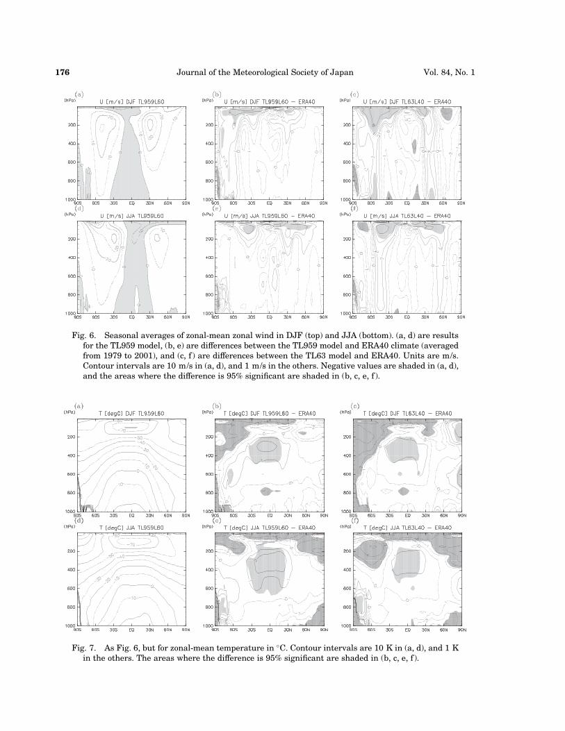
Fig. 6. Seasonal averages of zonal-mean zonal wind in DJF (top) and JJA (bottom). (a, d) are resultsfor the TL959 model, (b, e) are differences between the TL959 model and ERA40 climate (averagedfrom 1979 to 2001), and (c, f ) are differences between the TL63 model and ERA40. Units are m/s.Contour intervals are 10 m/s in (a, d), and 1 m/s in the others. Negative values are shaded in (a, d),and the areas where the difference is 95% significant are shaded in (b, c, e, f ).

Fig. 7. As Fig. 6, but for zonal-mean temperature in �C. Contour intervals are 10 K in (a, d), and 1 Kin the others. The areas where the difference is 95% significant are shaded in (b, c, e, f ).


latent heat transport, and enhanced precipita-tion in the tropics as shown in Figs. 1, 2 andTable 1.

Temperature in the lower and middle strato-sphere is lower than the ERA40 climate. Sincethe stratosphere involves large interannualvariabilities, it is necessary to perform manyyears of integration for comparing with the ob-servational climatology. For that reason, thestratosphere were left ‘‘untuned’’ in the presentversion of the model. Resolution dependence ofthe stratospheric temperature is smaller thanthe difference from the analysis.

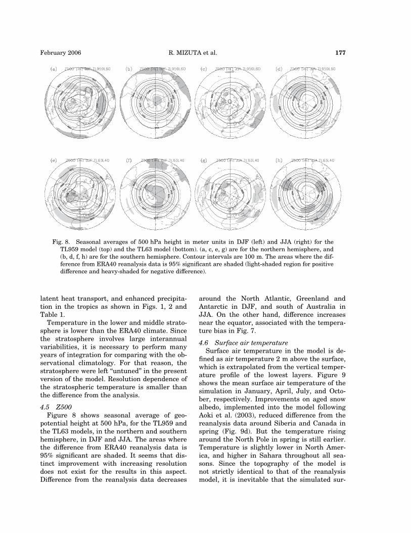
4.5 Z500Figure 8 shows seasonal average of geo-

potential height at 500 hPa, for the TL959 andthe TL63 models, in the northern and southernhemisphere, in DJF and JJA. The areas wherethe difference from ERA40 reanalysis data is95% significant are shaded. It seems that dis-tinct improvement with increasing resolutiondoes not exist for the results in this aspect.Difference from the reanalysis data decreases

around the North Atlantic, Greenland andAntarctic in DJF, and south of Australia inJJA. On the other hand, difference increasesnear the equator, associated with the tempera-ture bias in Fig. 7.

4.6 Surface air temperatureSurface air temperature in the model is de-

fined as air temperature 2 m above the surface,which is extrapolated from the vertical temper-ature profile of the lowest layers. Figure 9shows the mean surface air temperature of thesimulation in January, April, July, and Octo-ber, respectively. Improvements on aged snowalbedo, implemented into the model followingAoki et al. (2003), reduced difference from thereanalysis data around Siberia and Canada inspring (Fig. 9d). But the temperature risingaround the North Pole in spring is still earlier.Temperature is slightly lower in North Amer-ica, and higher in Sahara throughout all sea-sons. Since the topography of the model isnot strictly identical to that of the reanalysismodel, it is inevitable that the simulated sur-

Fig. 8. Seasonal averages of 500 hPa height in meter units in DJF (left) and JJA (right) for theTL959 model (top) and the TL63 model (bottom). (a, c, e, g) are for the northern hemisphere, and(b, d, f, h) are for the southern hemisphere. Contour intervals are 100 m. The areas where the dif-ference from ERA40 reanalysis data is 95% significant are shaded (light-shaded region for positivedifference and heavy-shaded for negative difference).


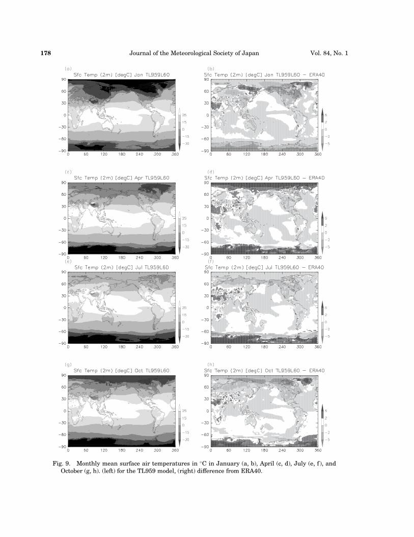
Fig. 9. Monthly mean surface air temperatures in �C in January (a, b), April (c, d), July (e, f ), andOctober (g, h). (left) for the TL959 model, (right) difference from ERA40.


face temperatures differ from the reanalysisdata associated with the difference of elevation,especially in mountain regions.

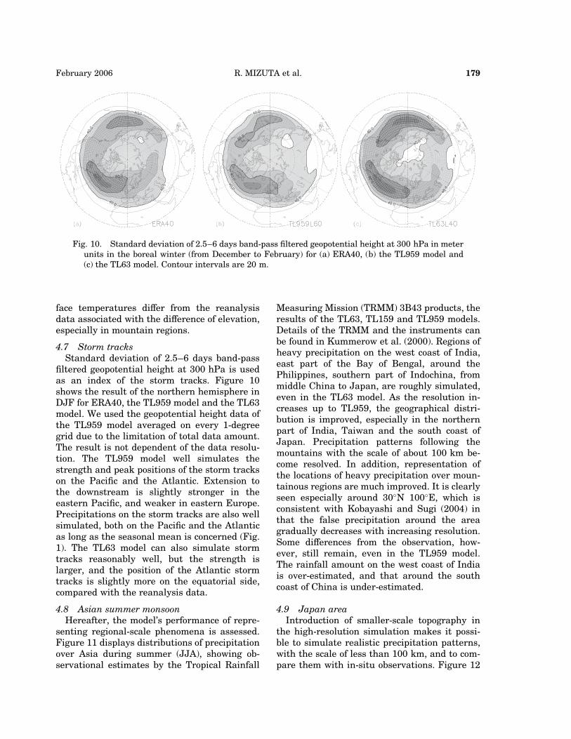
4.7 Storm tracksStandard deviation of 2.5–6 days band-pass

filtered geopotential height at 300 hPa is usedas an index of the storm tracks. Figure 10shows the result of the northern hemisphere inDJF for ERA40, the TL959 model and the TL63model. We used the geopotential height data ofthe TL959 model averaged on every 1-degreegrid due to the limitation of total data amount.The result is not dependent of the data resolu-tion. The TL959 model well simulates thestrength and peak positions of the storm trackson the Pacific and the Atlantic. Extension tothe downstream is slightly stronger in theeastern Pacific, and weaker in eastern Europe.Precipitations on the storm tracks are also wellsimulated, both on the Pacific and the Atlanticas long as the seasonal mean is concerned (Fig.1). The TL63 model can also simulate stormtracks reasonably well, but the strength islarger, and the position of the Atlantic stormtracks is slightly more on the equatorial side,compared with the reanalysis data.

4.8 Asian summer monsoonHereafter, the model’s performance of repre-

senting regional-scale phenomena is assessed.Figure 11 displays distributions of precipitationover Asia during summer (JJA), showing ob-servational estimates by the Tropical Rainfall

Measuring Mission (TRMM) 3B43 products, theresults of the TL63, TL159 and TL959 models.Details of the TRMM and the instruments canbe found in Kummerow et al. (2000). Regions ofheavy precipitation on the west coast of India,east part of the Bay of Bengal, around thePhilippines, southern part of Indochina, frommiddle China to Japan, are roughly simulated,even in the TL63 model. As the resolution in-creases up to TL959, the geographical distri-bution is improved, especially in the northernpart of India, Taiwan and the south coast ofJapan. Precipitation patterns following themountains with the scale of about 100 km be-come resolved. In addition, representation ofthe locations of heavy precipitation over moun-tainous regions are much improved. It is clearlyseen especially around 30�N 100�E, which isconsistent with Kobayashi and Sugi (2004) inthat the false precipitation around the areagradually decreases with increasing resolution.Some differences from the observation, how-ever, still remain, even in the TL959 model.The rainfall amount on the west coast of Indiais over-estimated, and that around the southcoast of China is under-estimated.

4.9 Japan areaIntroduction of smaller-scale topography in

the high-resolution simulation makes it possi-ble to simulate realistic precipitation patterns,with the scale of less than 100 km, and to com-pare them with in-situ observations. Figure 12

Fig. 10. Standard deviation of 2.5–6 days band-pass filtered geopotential height at 300 hPa in meterunits in the boreal winter (from December to February) for (a) ERA40, (b) the TL959 model and(c) the TL63 model. Contour intervals are 20 m.


Fig. 11. Seasonal mean precipitation over Asian monsoon region in units of mm/day in JJA, for (a)the average from 1998 to 2002 estimated from TRMM 3B43, (b) for the TL63 model, (c) for theTL159 model, and (d) for the TL959 model. Note that TRMM 3B43 dataset covers only the equa-torial side of 40 degrees north/south. Vectors in (b), (c), and (d) shows seasonal mean wind velocityat 850 hPa.

Fig. 12. Monthly mean precipitation over Japan in January. (a) 10-year-average from 1991 to 2000for Radar-AMeDAS analysis, (b) 10-year-average for the TL959 model.


shows monthly mean precipitation around theJapan area in January. Figure 12a is an esti-mation of the radar-AMeDAS precipitationanalysis averaged for 10 years. The radar-AMeDAS precipitation analysis is a datasetcovering the Japan Islands and its coastal re-gions. It is estimated from observations ofradars calibrated using densely distributed(about 17-km mesh) rain gauges. The calibra-tion algorithm is described in Makihara (1996).The spatial resolution is approximately 5 km.In winter, a large amount of snow is observedon the northwest coast of Japan, due to steadywinter monsoon northwesterlies from the Eur-asian continent blocked by the topography ofthe Japan Islands. The results of the TL959model presented in Fig. 12b show the modelcan simulate such detailed distributions of pre-cipitation on the northwest coast of Japan.

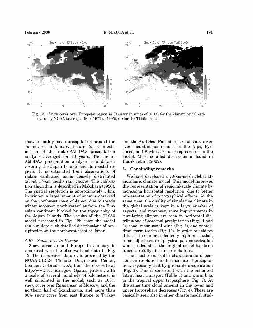
4.10 Snow cover in EuropeSnow cover around Europe in January is

compared with the observational data in Fig.13. The snow-cover dataset is provided by theNOAA-CIRES Climate Diagnostics Center,Boulder, Colorado, USA, from their website athttp://www.cdc.noaa.gov/. Spatial pattern, witha scale of several hundreds of kilometers, iswell simulated in the model, such as 100%snow cover over Russia east of Moscow, and thenorthern half of Scandinavia, and more than30% snow cover from east Europe to Turkey

and the Aral Sea. Fine structure of snow coverover mountainous regions in the Alps, Pyr-enees, and Kavkaz are also represented in themodel. More detailed discussion is found inHosaka et al. (2005).

5. Concluding remarks

We have developed a 20-km-mesh global at-mospheric climate model. This model improvesthe representation of regional-scale climate byincreasing horizontal resolution, due to betterrepresentation of topographical effects. At thesame time, the quality of simulating climate inthe global scale is kept in a large number ofaspects, and moreover, some improvements insimulating climate are seen in horizontal dis-tributions of seasonal precipitation (Figs. 1 and2), zonal-mean zonal wind (Fig. 6), and winter-time storm tracks (Fig. 10). In order to achievethis at the unprecedentedly high resolution,some adjustments of physical parameterizationwere needed since the original model has beentuned carefully at coarse resolutions.

The most remarkable characteristic depen-dent on resolution is the increase of precipita-tion, especially that by grid-scale condensation(Fig. 3). This is consistent with the enhancedlatent heat transport (Table 1) and warm biasin the tropical upper troposphere (Fig. 7). Atthe same time cloud amount in the lower andupper troposphere decreases (Fig. 4). These arebasically seen also in other climate model stud-

Fig. 13. Snow cover over European region in January in units of %. (a) for the climatological esti-mates by NOAA (averaged from 1971 to 1995), (b) for the TL959 model.


ies (e.g., Kiehl and Williamson 1991), althoughsub-grid scale parameterizations are differentwith each other.

The model’s performance of simulating theIndian and East Asian summer monsoons im-proves with finer resolution, consistent withprevious studies (Tibaldi et al. 1990; Sperber etal. 1994; Stephenson et al. 1998; Kobayashi andSugi 2004). Improvement is found not only inthe locations of precipitation, but also in quan-titative aspect. Details about this issue are notpresented here but can be found in Kusunokiet al. (2005).

This paper is intended to demonstrate acapability of simulating large-scale, seasonal-mean climate state, even in such a high-resolution model. The model thus enables usto study global characteristics of small-scalephenomena and extreme events. It is also pos-sible to focus on regions where regional climatemodels could not cover. A number of analyseson the small-scale issues have been, or areplanned to be, reported in separate publica-tions, including tropical cyclones (Oouchi et al.2005), Baiu fronts (Kusunoki et al. 2005), indi-ces of extreme events (Kamiguchi et al. 2005;Mizuta et al. 2005), and diurnal cycles of pre-cipitation (Arakawa et al. 2005). These phe-nomena have been found to be simulated wellin this model. Note that the treatment of seaice has room for improvement, since a moresophisticated scheme used in the previous cli-mate model of MRI has not been implementedin the present model. Therefore, care must betaken when one interprets the simulated re-sults relevant to sea ice.

We have already performed four sets of cli-mate simulations of over 10 years, using the20-km-mesh model: 1) a present-day climatesimulation using the observed climatologicalsea surface temperature (SST) as boundaryconditions (10 years), 2) a global warmingsimulation forced by climatological SST plusanomalies around the year 2090 obtained fromatmosphere-ocean coupled model simulations(10 years), 3) a present-day climate simulation(1979–1998) forced by the SST from a coupledmodel simulation (20 years), and 4) a globalwarming simulation (2080–2099) forced by theSST from a coupled model simulation (20years). In this paper, only the results about themean climate states of 1) were presented to ex-

amine fundamental performance of simulatingthe present-day climate. The results comparingthese experiments for projection of globalwarming are also reported in the publicationsmentioned above. At the same time, simu-lations with a nonhydrostatic regional climatemodel have been performed (Yoshizaki et al.2005; Yasunaga et al. 2005), of which lateralboundary conditions are provided by the calcu-lations of this paper. They focus on East Asiansummer monsoon, with horizontal grid size of5 km.

The resolution used in the present model isalmost the highest limit at which the pa-rameterizations including cumulus convectiveschemes work in expected manner as in thecoarser-resolution models. Based on a theoreti-cal inference, hydrostatic approximation seemsto be valid in this horizontal resolution, butmay be violated in the higher-resolution model.At that stage, nonhydrostatic cloud-resolvingglobal model will be necessary.

Acknowledgments

This work is a part of the ‘‘Kyosei Project 4:Development of Super High Resolution Globaland Regional Climate Models’’ supported byMinistry of Education, Culture, Sports, Scienceand Technology (MEXT). The developmentsand calculations were carried out by theKyosei-4 global modeling group. The authorswould like to thank Prof. A. Arakawa, Dr. T.Tokioka, Dr. K. Ninomiya and Dr. K. Masudafor comments on the earlier version of the high-resolution model, and Earth Simulator Centerfor providing computational environments.GFD-DENNOU Library are used for the draw-ings. The authors also thank two anonymousreviewers whose comments improved themanuscript.

References

Aoki, T., A. Hachikubo, and M. Hori, 2003: Effectsof snow physical parameters on shortwavebroadband albedos. J. Geophys. Res., 108(D19),4616, doi:10.1029/2003JD003506.

Arakawa, A. and W.H. Schubert, 1974: Interaction ofcumulus cloud ensemble with the large-scaleenvironment. Part I. J. Atmos. Sci., 31, 674–701.

Arakawa, O. and A. Kitoh, 2005: Rainfall diurnalvariation over the Indonesian Maritime Conti-


nent simulated by 20 km-mesh GCM. SOLA, 1,109–112.

Brankovic, C. and D. Gregory, 2001: Impact of hori-zontal resolution on seasonal integrations. Cli-mate Dyn., 18, 123–143.

Duffy, P.B., B. Govindasamy, J.P. Iorio, J. Milovich,K.R. Sperber, K.E. Taylor, M.F. Wehner, andS.L. Thompson, 2003: High-resolution simu-lations of global climate, part 1: present cli-mate. Climate Dyn., 21, 371–390.

Gravel, S. and A. Staniforth, 1994: A mass-conserving semi-Lagrangian scheme for theshallow water equations. Mon. Wea. Rev., 122,243–248.

Gregory, D., R. Kershaw, and P.M. Innes, 1997:Parameterization of momentum transport byconvection. II: Tests in single-column and gen-eral circulation models. Quart. J. Roy. Meteor.Soc., 123, 1153–1183.

Habata, S., K. Umezawa, M. Yokokawa, and S. Kita-waki, 2004: Hardware system of the EarthSimulator. Parallel Computing, 30, 1287–1313.

Harrison, E.F., P. Minnis, B.R. Barkstrom, V. Ram-anathan, R.D. Cess, and G.G. Gibson, 1990:Seasonal variation of cloud radiative forcingderived from the Earth Radiation Budget Ex-periment. J. Geophys. Res., 95, 18,687–18,703.

Hortal, M., 2002: The development and testing ofa new two-time-level semi-Lagrangian scheme(SETTLS) in the ECMWF forecast model.Quart. J. Roy. Meteor. Soc., 128, 1671–1687.

Hosaka, M., D. Nohara, and A. Kitoh, 2005: Changesin snow cover and snow water equivalent dueto global warming simulated by a 20 km-meshglobal atmospheric model. SOLA, 1, 93–96.

Huffman, G.J., R.F. Adler, P. Arkin, A. Chang, R.Ferraro, A. Gruber, J. Janowiak, A. McNab,and B. Schneider, 1997: The Global Precipita-tion Climatology Project (GPCP) combinedprecipitation data set. Bull. Amer. Meteor. Soc.,78, 5–20.

IPCC, 2001: Climate Change 2001: The ScientificBasis. J.T. Houghton et al. Eds., CambridgeUniversity Press, UK, 881 pp.

Iwasaki, T., S. Yamada, and K. Tada, 1989: A pa-rameterization scheme of orographic gravitywave drag with the different vertical partition-ing, part 1: Impact on medium range forcast. J.Meteor. Soc. Japan, 67, 11–41.

JMA, 2002: Outline of the operational numericalweather prediction at the Japan MeteorologicalAgency (Appendix to WMO numerical weatherprediction progress report). Japan Meteorolog-ical Agency, 157pp. (available online at http://www.jma.go.jp/JMA_HP/jma /jma-eng/jma-center/nwp/outline-nwp/index.htm)

Kamiguchi, K., A. Kitoh, T. Uchiyama, R. Mizuta,and A. Noda, 2005: Changes in precipitation-based extremes indices due to global warmingprojected by a global 20-km-mesh atmosphericmodel. SOLA, submitted.

Kanamitsu, T., K. Tada, T. Kudo, N. Sato, and S. Isa,1983: Description of the JMA operational spec-tral model. J. Meteor. Soc. Japan, 61, 812–828.

Kawai, H., 2003: Impact of a cloud ice fall schemebased on an analytically integrated solution.CAS/JSC WGNE Research Activities in Atmo-spheric and Ocean Modeling, 33, 4.11–4.12.

———, 2004: Impact of a parameterization for sub-tropical marine stratocumulus. CAS/JSCWGNE Research Activities in Atmospheric andOcean Modeling, 34, 4.13–4.14.

———, 2005: Improvement of a cloud ice fall schemein GCM. CAS/JSC WGNE Research Activitiesin Atmospheric and Ocean Modeling, 35, 4.11–4.12.

Kiehl, J.T. and K.E. Trenberth, 1997: Earth’s annualglobal mean energy budget. Bull. Amer. Me-teor. Soc., 78, 197–208.

——— and D.L. Williamson, 1991: Dependence ofcloud amount on horizontal resolution in theNational Center for Atmospheric ResearchCommunity Climate Model. J. Geophys. Res.,96, 10,955–10,980.

Kobayashi, C. and M. Sugi, 2004: Impact of horizon-tal resolution on the simulation of the Asiansummer monsoon and tropical cyclones in theJMA global model. Climate Dyn., 93, 165–176.

Kusunoki, S., J. Yoshimura, H. Yoshimura, A. Noda,K. Oouchi, and R. Mizuta, 2005: Change ofBaiu in global warming projection by an atmo-spheric general circulation model with 20-kmgrid size. J. Meteor. Soc. Japan. submitted.

Kummerow, C. and Coauthors, 2000: The statusof the Tropical Rainfall Measuring Mission(TRMM) after two years in orbit. J. Appl. Me-teor., 39, 1965–1982.

Makihara, Y., 1996: A method for improving radarestimates of precipitation by comparing datafrom radars and raingauges. J. Meteor. Soc.Japan, 74, 459–480.

Mellor, G.L. and T. Yamada, 1974: A hierarchy ofturbulence closure models for planetaryboundary layers. J. Atmos. Sci., 31, 1791–1806.

Mizuta, R., T. Uchiyama, K. Kamiguchi, A. Kitoh,and A. Noda, 2005: Changes in extremes indi-ces over Japan due to global warming projectedby a global 20-km-mesh atmospheric model.SOLA, 1, 153–156.

Moorthi, S. and M.J. Suarez, 1992: RelaxedArakawa-Schubert: A parameterization ofmoist convection for general circulationmodels. Mon. Wea. Rev., 120, 978–1002.


Nakagawa, M. and A. Shimpo, 2004: Developmentof a cumulus parameterization scheme for theoperational global model at JMA. RSMCTokyo-Typhoon Center Techninal Review, 7,10–15.

Ohfuchi, W., H. Nakamura, M.K. Yoshioka, T. Eno-moto, K. Takaya, X. Peng, S. Yamane, T. Nish-imura, Y. Kurihara, and K. Ninomiya, 2004:10-km mesh meso-scale resolving simulationsof the global atmosphere on the Earth Simula-tor—preliminary outcomes of AFES (AGCMfor the Earth Simulator)—, J. Earth Simula-tor, 1, 8–34.

Oouchi, K., J. Yoshimura, H. Yoshimura, R. Mizuta,S. Kusunoki, and A. Noda, 2006: Tropical cy-clone climatology in a global-warming climateas simulated in a 20 km-mesh global atmo-spheric model. J. Meteor. Soc. Japan, in press.

Pan, D.-M. and D. Randall, 1998: A cumulus param-eterization with a prognostic closure. Quart. J.Roy. Meteor. Soc., 124, 949–981.

Phillips, T.J., L.C. Corsetti, and S.L. Grotch, 1995:The impact of horizontal resolution on moistprocesses in the ECMWF model. Climate Dyn.,11, 85–102.

Pope, V.D. and R.A. Stratton, 2002: The processesgoverning horizontal resolution sensitivity in aclimate model. Climate Dyn., 19, 211–236.

Priestley, A., 1993: A quasi-conservative version ofthe semi-Lagrangian advection scheme. Mon.Wea. Rev., 121, 621–629.

Randall, D. and D.-M. Pan, 1993: Implementation ofthe Arakawa-Schubert cumulus parameter-ization with a prognostic closure. Meteorologi-cal Monograph/The representation of cumulusconvection in numerical models, 46, 145–150.

Reynolds, R.W. and T.M. Smith, 1994: Improvedglobal sea surface temperature analysis usingoptimum interpolation. J. Climate., 7, 929–948.

Ritchie, H., C. Temperton, A. Simmons, M. Hortal, T.Davies, D. Dent, and M. Hamrud, 1995: Imple-mentation of the semi-Lagrangian method in ahigh-resolution version of the ECMWF forecastmodel. Mon. Wea. Rev., 123, 489–514.

Sellers, P.J., Y. Mints, Y.C. Sud, and A. Dalcher,1986: A simple biosphere model (SiB) for usewithin general circulation models. J. Atmos.Sci., 43, 505–531.

Shibata, K., H. Yoshimura, M. Ohizumi, M. Hosaka,and M. Sugi, 1999: A simulation of tropo-sphere, stratosphere and mesosphere with anMRI/JMA98 GCM. Pap. Meteor. Geophys., 50,15–53.

Simmons, A.J. and Gibson, J.K., 2000: The ERA-40Project Plan, ERA-40 Project Report Series 1.ECMWF. Shinfield Park, Reading, UK, 63pp.

Slingo, J.M., 1987: The development and verificationof a cloud prediction scheme in the ECMWFmodel. Quart. J. Roy. Meteor. Soc., 113, 899–927.

Smith, R.N.B., 1990: A scheme for predicting layerclouds and their water content in a generalcirculation model. Quart. J. Roy. Meteor. Soc.,116, 435–460.

Sommeria, G. and J.W. Deardorff, 1977: Subgrid-scale condensation in models of nonprecipi-tating clouds. J. Atmos. Sci., 34, 344–355.

Sperber, K.R., S. Hamed, G.L. Potter, and J.S. Boyle,1994: Simulation of the northern summermonsoon in the ECMWF model: sensitivity tohorizontal resolution. Mon. Wea. Rev., 122,2461–2481.

Stephenson, D.B., F. Chauvi, and J.-F. Royer, 1998:Simulation of the Asian Summer Monsoon andits dependence on model horizontal resolution.J. Meteor. Soc. Japan, 76, 237–265.

Stratton, R.A., 1999: A high resolution AMIP in-tegration using the Hadley Centre model Ha-dAM2b. Climate Dyn., 15, 9–28.

Sundqvist, H., 1978: A parameterization scheme fornon-convective condensation including predic-tion of cloud water content. Quart. J. Roy. Me-teor. Soc., 104, 677–690.

Tanaka, T.Y., Orito, K., Sekiyama, T., Shibata, K.,Chiba, M., and Tanaka, H., 2003: MASINGAR,a global tropospheric aerosol chemical trans-port model coupled with MRI/JMA98 GCM:Model description. Pap. Meteor. Geophys., 53,119–138.

Temperton, C., M. Hortal, and A.J. Simmons, 2001:A two-time-level semi-Lagrangian global spec-tral model. Quart. J. Roy. Meteor. Soc., 127,111–127.

Tibaldi, S., T.N. Palmer, C. Brankovic, and U. Cu-basch, 1990: Extended range predictions withECMWF models: influence of horizontal reso-lution on systematic error and forecast skill.Quart. J. Roy. Meteor. Soc., 116, 835–866.

Williamson, D.L., J.T. Kiehl, and J.J. Hack, 1995:Climate sensitivity of the NCAR CommunityClimate model (CCM2) to horizontal resolu-tion. Climate Dyn., 11, 377–397.

Wu, X. and M. Yanai, 1994: Effects of vertical windshear on the cumulus transport of momentum:Observations and parameterization. J. Atmos.Sci., 51, 1640–1660.

Xie, P. and P.A. Arkin, 1997: Global precipitation: a17-year monthly analysis based on gauge ob-servations, satellite estimates, and numericalmodel outputs. Bull. Amer. Meteor. Soc., 78,2539–2558.

Yasunaga, K., M. Yoshizaki, Y. Wakazuki, C. Muroi,K. Kurihara, A. Hashimoto, S. Kanada, T.


Kato, S. Kusunoki, K. Oouchi, H. Yoshimura,R. Mizuta, and A. Noda, 2006: Changes in theBaiu frontal activity in the global warmingclimate simulated by super-high-resolutionglobal and cloud-resolving regional models. J.Meteor. Soc. Japan, 84, 199–220.

Yoshimura, H. and T. Matsumura, 2003: A semi-Lagrangian scheme conservative in the verticaldirection. CAS/JSC WGNE Research Activitiesin Atmospheric and Ocean Modeling, 33, 3.19–3.20.

——— and T. Matsumura, 2005: A two-time-levelvertically-conservative semi-Lagrangian semi-implicit double Fourier series AGCM. CAS/JSCWGNE Research Activities in Atmospheric andOcean Modeling, 35, 3.27–3.28.

Yoshizaki, M., C. Muroi, S. Kanada, Y. Wakazuki, K.Yasunaga, A. Hashimoto, T. Kato, K. Kurihara,A. Noda, and S. Kusunoki, 2005: Changesof Baiu (Mei-yu) frontal activity in theglobal warming climate simulated by a non-hydrostatic regional model. SOLA, 1, 25–28.


20-km-Mesh Global Climate Simulations Using JMA-GSM Model ...

Documents

Transcript of 20-km-Mesh Global Climate Simulations Using JMA-GSM Model ...