20 century drought in the conterminous United … et al. 1 20 th century drought in the conterminous...
49
Andreadis et al. 1 20 th century drought in the conterminous United States Konstantinos M. Andreadis 1 , Elizabeth A. Clark 1 , Andrew W. Wood 1 , Alan F. Hamlet 1 , and Dennis P. Lettenmaier 1 1 Department of Civil and Environmental Engineering, Box 352700, University of Washington, Seattle, WA 98195; (206)543-2532; [email protected]
Transcript of 20 century drought in the conterminous United … et al. 1 20 th century drought in the conterminous...

Andreadis et al.
1
20th century drought in the conterminous United States
Konstantinos M. Andreadis1, Elizabeth A. Clark1, Andrew W. Wood1, Alan F. Hamlet1,
and Dennis P. Lettenmaier1
1Department of Civil and Environmental Engineering, Box 352700, University of
Washington, Seattle, WA 98195; (206)543-2532; [email protected]

Andreadis et al.
2
Abstract
Droughts can be characterized by their severity, frequency and duration, and areal
extent. Depth-area-duration analysis, widely used to characterize precipitation extremes,
provides a basis for evaluation of drought severity when storm depth is replaced by an
appropriate measure of drought severity. We used gridded precipitation and temperature
data to force a physically-based macroscale hydrologic model at 1/2o spatial resolution
over the continental U.S., and then constructed a drought history from 1920 to 2003
based on the model-simulated soil moisture and runoff. A clustering algorithm was used
to identify individual drought events and their spatial extent from monthly summaries of
the simulated data. A series of severity-area-duration (SAD) curves were constructed to
relate the area of each drought to its severity. An envelope of the most severe drought
events in terms of their SAD characteristics was then constructed. Our results show that
a) the droughts of the 1930s and 1950s were the most severe of the 20th century for large
areas; b) the early 2000s drought in the western U.S. is among the most severe in the
period of record, especially for small areas and short durations; c) the most severe
agricultural droughts were also among the most severe hydrologic droughts – however,
the early 2000s western U.S. drought occupies a larger portion of the hydrologic drought
envelope curve than does its agricultural companion; d) runoff tends to recover in
response to precipitation more quickly than soil moisture, so the severity of hydrologic
drought during the 1930s and 1950s was dampened by short wet spells while the severity
of the early 2000s drought remained high due to the relative absence of these short term
phenomena.

Andreadis et al.
3
1. Introduction
Drought is among the most costly natural disasters. In 1995, the U.S. Federal
Emergency Management Agency (FEMA, 1995) estimated that the annual cost of U.S.
droughts was in the range of $6-8B. According to NOAA's National Climate Data Center
(2003), the 1988 drought alone, cost nearly $62B (in 2002 dollars), making it the most
costly natural disaster in U.S. history. Webb et al. (2004) suggest that the recent western
U.S. drought could be the most severe in the last 500 years, based on tree ring analysis.
Dai et al. (2004) report a tendency towards more extreme droughts over the past two to
three decades due to global warming. Furthermore, the drying of soils associated with
this warming enhances the risk of long duration droughts.
To assess the potential impacts of drought, water managers often compare current
or potential drought severity for a given location (or river basin) with the severity of
historical droughts. However, this approach overlooks the effects of areal extent on
drought intensity. The potential for costly and widespread drought conditions argues for
the development of more comprehensive methods for drought characterization.
The overall impact of a drought depends on several factors, including not only its
severity, but also frequency, area, and duration. Several drought indices have been
defined (primarily for the characterization of drought severity), which typically describe
one of four drought types: agricultural, hydrologic, meteorological, and socioeconomic.
Generally, agricultural drought is related to soil moisture, hydrologic drought to runoff
and streamflow, meteorological drought to precipitation, and socioeconomic drought to
the disparity between supply and demand for water (Wilhite and Glantz 1985). This paper
focuses on agricultural and hydrologic drought over the continental U.S.

Andreadis et al.
4
For long-term drought characterization, the Palmer Drought Severity Index
(PDSI; Palmer 1965) is the most widely used drought index. PDSI is a measure of
meteorological drought; however, the method accounts for evapotranspiration and soil
moisture conditions as well as precipitation, both of which are determinants of hydrologic
drought (Alley 1984) therefore it is related to hydrologic (and agricultural) drought as
well. Dai et al. (2004) report correlations between annual PDSI and streamflow globally.
They also find a positive correlation between PDSI and soil moisture during warm
seasons at a regional or river-basin scale, although they note that PDSI should not be used
as a measure of soil moisture in cold seasons or at high latitudes because snow interferes
with soil moisture calculations in PDSI. For these (and other) reasons, PDSI is generally
considered inadequate for characterization of agricultural or hydrologic drought.
Nonetheless, the attraction to PDSI is its standardization, which theoretically
should enable comparisons of drought intensity across heterogeneous regions. Palmer
(1965) provides a clear indication of how the initialization and termination of drought can
be estimated using PDSI. However, PDSI values are highly sensitive to termination
criteria, which are somewhat arbitrary (Alley 1984). As a result, spatial patterns of PDSI
sometimes defy physical explanation, with some areas commonly experiencing severe
droughts and others rarely experiencing drought (Willeke et al., 1994) despite climate
conditions that would suggest otherwise. Although other drought indicators, such as soil
moisture in the case of agricultural drought or runoff as a measure of hydrologic drought,
reflect an adequate physical basis for interpretation, they are often constrained by data
availability.
Soulé (1993) notes that when analyzing drought trends, fine-scale data should be
used to account for the spatial heterogeneity of drought patterns. Because stream gauges

Andreadis et al.
5
integrate over relatively large spatial areas (especially in the case of the relatively small
number of gages that have been operated continuously for half a century or more), and
because stream gauges are often located to benefit water resources operations, they do not
generally resolve spatial variability of hydrologic drought adequately. Long-term soil
moisture data (i.e., records longer than a few decades) are virtually non-existent in the
U.S. (except in Illinois and Iowa, Robock et al. 2000), hence direct estimation of long-
term statistics of agricultural drought for the continental U.S. is essentially impossible.
These factors are a major reason for the widespread use of PDSI, despite its known
shortcomings. A standard approach to mapping drought is to assign a single PDSI value,
based on station data, to each of 344 climatic divisions of the contiguous U.S. (e.g. Soulé
1993). Alternately, several studies have interpolated tree-ring chronologies to produce
gridded PDSI data sets, thereby extending the record of drought as far back as 1700 (Karl
and Koscielny 1982; Cook et al. 1999).
An alternative to these methods is to use physically-based hydrologic models to
simulate variables (soil moisture; runoff) from which agricultural and hydrologic drought
can be computed using consistent gridded data sets of the model meteorological forcings.
The output of these models can be used to map the spatial extent of drought. NOAA's
Climate Prediction Center (CPC, 2005), for example, estimates soil moisture, evaporation
and runoff from observed temperature and precipitation using a one-layer hydrological
model (Huang et al. 1996). Although spatially contiguous data sets of relevant parameters
have been developed, relationships between the area of an individual drought event and
its severity have not been fully explored.
The U.S. Drought Monitor (2003) produces maps of drought extent and severity
using a combination of several drought indicators, including PDSI, CPC simulated soil

Andreadis et al.
6
moisture (percentiles), U.S. Geological Survey weekly observed streamflow (percentiles),
standardized precipitation index, and a satellite vegetation health index. The weighting of
these indicators combines objective and subjective characterization techniques to reflect
conditions in various regions and at different times of year. CPC is also experimenting
with more objective blends of drought indicators as a supplemental tool.
Following the CPC, we employ a macroscale hydrologic model to simulate soil
moisture and runoff for the conterminous U.S.. Rather than using climate division data,
we perform a retrospective analysis of historical droughts from 1920 through 2003 using
recently released digitized Cooperative Observer Network (Co-op) station data from
NOAA's National Climate Data Center (NCDC), which we grid to one-half degree spatial
resolution. For simplicity, and to maintain objectivity in the weighting of factors, we use
soil moisture percentile anomalies as an indicator of agricultural drought severity. The
relative severity of agricultural droughts is then compared with that of hydrologic drought
as designated by runoff percentile anomalies.
The purpose of this study is to identify the major drought events of the 20th
century in the continental U.S. based not only on their severity, but also on their areal
extent and duration. Several studies have used principal component analysis of gridded
PDSI, derived from historical climate data, to delineate spatially homogeneous areas of
drought and to relate these to global-scale climate patterns, such as the El Niño Southern
Oscillation or the Pacific Decadal Oscillation (e.g. Karl and Koscielny 1982; Dai et al.
1998; Dai et al. 2004; Schubert et al. 2004). Fewer studies have examined the relative
extent of individual drought events or the relationship between drought severity and areal
extent. Sheffield et al. (2004) have evaluated drought severity and extent using

Andreadis et al.
7
macroscale simulation model output similar to ours, but with somewhat different
analytical methods.
Others have used historical drought records to relate drought severity to duration
and frequency. Dalezios et al. (2000) developed a severity-duration-frequency analysis,
using PDSI data for 1957-1983, based on intensity-duration-frequency relationships that
are typically used to synthesize design-storms. We adapt another tool typically used to
characterize storm precipitation: depth-area-duration (DAD) analysis (WMO, 1969). For
drought analysis we simply replace depth of precipitation with a measure of drought
severity. In so doing, we take advantage of the high resolution spatial data, simulated by a
physically-based hydrologic model, to include area in our definition of drought intensity.
We will refer to this technique as severity-area-duration analysis (SAD).
2. Data set description
The recent availability of Cooperative Observer station meteorological daily data
(DSI-3206) for the pre-1949 period enabled extension of our analysis from the 1950-2000
period used by Sheffield et al. (2004) (based in turn on the derived hydrologic data
archive for the continental U.S. described by Maurer et al. (2002)) to encompass the early
20th century as well. The NCDC now maintains electronic archives of digitized versions
of all data provided by its Cooperative Observers within the 50 states, as well as in Puerto
Rico and the U.S. Virgin Islands. We merged these data with a previously released
cooperative station data set (DSI-3200) to create a continuous record for the 1915 to 2003
period. Like DSI-3200, DSI-3206 includes air temperature with observation times at 7
am, 2 pm, and 9 pm; daily maximum, minimum and mean temperatures; total
precipitation, snowfall, and depth of snow on ground; prevailing wind direction and total
Andreadis et al.
8
wind movement; evaporation; sky condition; and occurrence of weather and obstructions
to vision (NCDC, 2003) – although the data density for precipitation and air temperature
maxima and minima is generally much higher than for the other variables. We gridded
data from 2489 stations for precipitation and 1904 for temperature to ½ degree spatial
resolution using methods outlined in Maurer et al. (2002) then aggregated the data to over
the North American Land Data Assimilation System (NLDAS) domain, which includes
all of North America from 25 to 53 degrees N latitude (Mitchell et al. 2004).
We applied methods described in Hamlet and Lettenmaier (2005) to correct for
temporal heterogeneities in the data. This method essentially adjusts the gridded data to
have decadal scale variability comparable to that of the U.S. Historical Climatology
Network (HCN) in the U.S. (and the Historical Canadian Climate Database (HCCD) in
Canada). HCN (Karl et al. 1990) and HCCD (Mekis and Hogg, 1999; Vincent et al,
1999) are high quality station data sets which have been carefully adjusted for effects of
changes in instrumentation and other factors not related to natural climate variability over
the period of record. The resultant adjusted data set reproduces the monthly precipitation
and temperature trends of the HCN and HCCD data, while retaining the spatial
information from the larger number of stations in the Co-op records. The final forcing
data set also includes a topographical precipitation correction described in Maurer et al.
(2002) based on the Precipitation Regression on Independent Slopes Method (PRISM)
precipitation maps (Daly et al. 1994).
3. Hydrology model description
We used the Variable Infiltration Capacity (VIC) model (Liang et al. 1994; 1996;
Cherkauer et al. 2003) to simulate historical soil moisture and runoff over the NLDAS

Andreadis et al.
9
domain. The VIC model balances energy and moisture fluxes over each grid cell (one
half degree latitude by longitude in this case). The model includes a soil-vegetation-
atmosphere transfer scheme (SVAT) which represents the controls exerted by vegetation
and soil moisture on land-atmosphere moisture and energy fluxes. VIC accounts for the
effects of sub-grid scale variability in soil, vegetation, precipitation, and topography on
grid scale fluxes. It represents the subsurface as three layers – a relatively thin surface
layer, from which surface or “fast” runoff is generated, and two progressively deeper
layers which control subsurface runoff generation. In this study, we used the same soils,
vegetation, and topographic data as in Maurer et al. (2002), aggregated to the one-half
degree spatial resolution. The Maurer et al. data are in turn quite similar to those used in
NLDAS (Mitchell et al. 2004).
Several studies have successfully simulated runoff and streamflow using the VIC
model over large river basins and at continental to global scales for multi-decadal periods
(e.g. Abdulla et al. 1996; Lohmann et al. 1998; Nijssen et al. 1997, 2001; Wood et al.
1997; Maurer et al. 2002). Nijssen et al. (2001) report good correspondence between the
annual cycle and spatial patterns of soil moisture simulated by VIC and the observed soil
moisture in central Illinois and in central Eurasia. Likewise, Maurer et al. (2002) find that
observed soil moisture persistence is better represented by the VIC model than the Huang
et al. (1996) model used by the U.S. Drought Monitor. They also note that over shorter
time-scales, VIC-derived soil moisture is well-suited for use in diagnostic studies.
Furthermore, Robock et al. (2003) showed good agreement of spatially averaged soil
moisture between VIC and Mesonet stations over the southern Great Plains, although
VIC underestimated the seasonal variation of soil moisture.
Andreadis et al.
10
For this study, the period for which simulations were performed was January
1915 through December 2003, using a daily time step in water balance mode (which
means that the surface temperature was set to surface air temperature, rather than being
iterated for energy balance closure). As in Maurer et al. (2002), soil depths varied from
0.1 to 0.5 m for the upper layer, 0.2 to 2.4 m for the middle layer, and 0.1 to 2.5 m for the
lower layer. Exploratory analysis indicated that as much as a decade is necessary to fully
remove the effects of initial soil moisture conditions, especially in dry regions. To
minimize the spinup period, we averaged January soil moisture values (to coincide with
the starting date of our simulations), from an uninitialized simulation for the period 1925
to 2003 and took these as initial soil moisture for subsequent runs. Exploratory analyses
have suggested that the soil moisture equilibration time required for VIC, ranges from 6
months (Cosgrove et al., 2003) to a decade. Therefore, we used the period 1915-1919 for
spin-up, and performed our analysis for the period 1920-2003.
4. Soil moisture and runoff percentiles
One approach to defining drought severity is to measure the degree of departure
from normal. In this paper, we use soil moisture anomalies as a measure of agricultural
drought and runoff anomalies as a measure of hydrologic drought. Our desire is to
develop a method that allows direct comparison of droughts across the domain. Use of
absolute magnitude (e.g., of soil moisture deficits) is not appropriate for this purpose
because anomalies in absolute terms reflect different severities in different parts of the
domain. The use of percentiles, which by construct have a range from zero to one (and
are uniformly distributed over this range) is more appropriate for our purposes.

Andreadis et al.
11
Monthly percentiles were calculated for each grid cell based on the climatology of
the 84 year study period. Soil moisture in each of the three soil layers was accumulated
for each month to produce a single value of total column soil moisture. Empirical
cumulative probability distributions were formed for each grid cell and each month for
soil moisture and runoff (using the Weibull plotting position), and the raw total column
soil moisture and runoff were replaced by their percentiles.
5. Drought identification in space and time
Fundamental descriptors of droughts include their intensity and duration (Dracup
et al. 1980b). Duration can be defined as the number of consecutive time steps that the
time series (of soil moisture or runoff) is below a specified threshold level (Byun and
Wilhite 1999), intensity as the averaged cumulative departure from the threshold level for
that duration, while severity is defined as the product of intensity and duration
(cumulative departure from the drought threshold). Because droughts are regional
phenomena that can cover large areas for long periods of time, the spatial extent of a
drought is an equally important feature. Most previous studies have focused their analysis
of the spatial patterns of drought on readily available point data (Soulé 1993). Statistical
methods, such as correlation analysis (Oladipo 1986) and empirical orthogonal functions
(EOF) have been used (Dai et al. 1998; 2004; Cook et al. 1999; Hisdal and Tallaksen
2003), to estimate the regional characteristics of droughts as estimated from point or
gridded data. These methods group stations that exhibit similar behavior in a statistical
sense, for regionalization purposes. In this paper, we instead exploit the areal estimates of
hydrologic variables provided by VIC simulations to evaluate drought extent. Our
simulations provide spatially and temporally continuous mapping of (transformed) soil
Andreadis et al.
12
moisture and runoff over our domain, and it is therefore possible to evaluate spatial
patterns of drought directly from the derived data, using methods outlined below.
An objective definition of drought events is elusive, and many have been given
depending on the context of the application. One of the most widely used methods for
drought classification is based on defining a threshold level below which a drought is said
to have occurred (Dracup et al. 1980a). An important aspect of this method is the
selection of the threshold (or truncation) value. The PDSI, for example, is highly
sensitive to termination criteria (Alley 1984). A relatively high moisture threshold, such
as the mean of a streamflow time series, would result in a large number of drought
events. Given the temporal and spatial dimensions of the study domain, it is more
appropriate to focus on moderate to extreme droughts. The CPC classifies droughts based
on simulated soil moisture percentiles (from a 70-year record, 1931-2000) amongst other
indicators, and uses the following classification scheme: moderate drought (11-20 %),
severe drought (6-10 %), extreme drought (3-5 %), and exceptional drought (0-2 %)
(U.S. Drought Monitor 2003; CPC 2005). Following this scheme, we define the
beginning and end of drought conditions based on a soil moisture (or runoff) percentile
value of 20%.
The spatial identification procedure is based on a simple clustering algorithm that
incorporates spatial contiguity. The process involves the initial partitioning of the data,
for each month of the time series, into a number of clusters, and the subsequent merging
of those based on minimum area constraints. Because droughts are regional phenomena,
it can be argued that the prominent spatial characteristic of a drought event is the
contiguity of its extent. Consequently, the distance between pixels that are under drought,
should facilitate the regionalization procedure.

Andreadis et al.
13
The algorithm begins with a spatial smoothing pre-processing step. The spatial
filter selected is a 3x3 median filter, which ensures minimum distortion of the original
data. At each monthly timestep, all pixels that have a soil moisture (or runoff) percentile
value below 20% are considered as being "under drought". Those pixels are then
classified into drought classes using a simple clustering algorithm. The first pixel under
drought is assigned to the first class. Then the 3x3 neighborhood of this pixel is searched
for pixels under drought which are classified in the same drought cluster. This procedure
is repeated until no pixels in the 3x3 neighborhood of the current pixel are under drought,
and a new cluster is created for the next pixel below the drought threshold. After the
initial partitioning step, the final classification step is to apply a minimum area threshold
to each cluster (taken here as 10 pixels). If a cluster contains less than 10 pixels, it is not
included in any of the subsequent calculations. At the end of this step, the remaining
clusters are defined as separate drought events for the current timestep.
Using this procedure, drought events are allowed to have variable duration and
spatial extent, and are not confined to a pre-defined climate region. Therefore, we have to
take into account the cases when multiple clusters merge to form a larger drought in later
time steps, or a drought event breaks up into multiple smaller droughts. In both cases, the
smaller droughts are considered part of the larger drought, but their spatial extents and
severities are calculated separately by imposing a contiguity constraint. This is
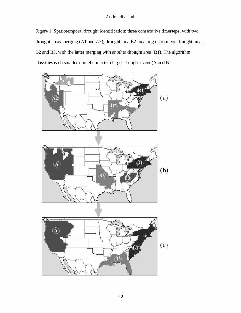
demonstrated in Figure 1, which shows how the algorithm classifies two drought events
for three consecutive time steps. In time step 1 (Figure 1a), there are four drought events.
The two droughts in the western U.S. however, merge into one spatially larger event in
time step 2 (Figure 1b), which also occupies the same area over the next time step.
Obviously the two drought areas (A1 and A2) in time step 1 should be considered as

Andreadis et al.
14
belonging to the same drought event. On the other hand, the drought area covering the
southeastern U.S. in time step 1 breaks off into two sub-droughts in time step 2 (B2 and
B3). These areas are classified in the same larger drought event, but their corresponding
severities are computed separately during the time steps during which they are not
spatially contiguous. In time step 3 (Figure 1c), one of the drought areas that broke off
merges with the drought over the northeastern region. Our approach is to re-classify all
these areas as belonging to the same larger event, on the basis that the driving climatic
variables are the same.
6. Construction of drought Severity-Area-Duration curves
DAD relationships of precipitation are used in engineering studies to estimate an
areal reduction factor (ARF) for the reduction of point to areal precipitation (Grebner and
Roesch 1997). This areal precipitation is then used in runoff volume computations to
determine design storms for design of small flood control structures (Dhar and Nandargi
1993). Just as depths of precipitation characterize extreme wet events, deficits of
moisture characterize extreme dry events. Based on the distribution of these deficits in
time and space, we can also characterize drought using its areal extent and duration.
Therefore, we translate the DAD approach to evaluate drought conditions by replacing
depth with a measure of severity. For the purposes of this paper, severity (S) is defined
as S=(1-ΣP/t)*100%, where ΣP is the monthly percentile of soil moisture or runoff
summed over duration t (with t in months). Because model output is gridded, we do not
need to construct isohyetal maps as is done in classical DAD analysis of storms. Instead,
we adapted the computational method of WMO (1969) to calculate the average severity
corresponding to each standard area. For this study, we examine durations of 3, 6, 9, 12,

Andreadis et al.
15
24, 36, 48, and 72 months and areas from 10 grid cells, or approximately 25,000 km2, to
the maximum drought extent of about 106 km2, in increments of 20 grid cells, or
approximately 50,000 km2.
The process used to calculate drought severity at each duration starts with the grid
cells being ranked by severity. Those cells with the maximum severity are used as
potential "drought centers," corresponding to the storm centers of DAD analysis. The 3-
by-3 neighborhood of the first drought center is identified, and the area of the
neighboring cell with the highest severity is added to that of the first. Their severities are
averaged, and the two cells collectively form an intermediate drought area. Then the cells
neighboring this intermediate drought area are identified, and the area of the cell with the
maximum severity is added to the intermediate drought area. Once the first standardized
area is reached, the severity and area are recorded. The process continues until all cells
areas under drought are summed and severities averaged.
Because the area surrounding the first drought center might not match the
maximum severity for a given area interval, we repeat this procedure on each of the
remaining drought centers. For each duration, the combination of concurrent months that
experienced the highest severity provides the severity for its corresponding area interval.
The resultant plots reflect a drought-centered, absolute SAD relationship, which can be
used to estimate absolute drought magnitudes without being constrained to an individual
basin or area (see Grebner and Roesch 1997).
After calculating SAD relationships for each drought event, we identify the
maximum severity events for each area interval and duration. These are used to
generalize an enveloping relationship of the most extreme drought events in the U.S.
between 1920 and 2003.

Andreadis et al.
16
7. Results
a. Soil moisture droughts
Based on the drought threshold selected for the soil moisture-based analysis
(20%), and the drought definition used in this study, 248 drought events were identified
over the simulation period (1920 to 2003). However, only four of these spanned the
maximum duration of our analysis (72 months), while most lasted for less than 6 months
(189 events). The longest droughts occurred during the 1930s (1932-1938), 1950s (1950-
1957), 1960s (1960-1967), and late 1980s (1987-1993); each of these had a duration of 6-
7 years. Other notably long events included events in 1975-1979, 1958-1962, 1998-2003,
and 1928-1932. With respect to spatial extent, the drought events that stand out occurred
during the 1930s and 1950s and covered almost the entire continental U.S. Not
surprisingly, other spatially expansive events coincided with the longest duration events,
but with differences in the relative order. In terms of spatial extent, they ranked, from
largest to smallest, as follows: 1987-93, 1998-2003, 1960-67, 1975-79, 1928-32 and
1938-41.
The spatial patterns of each of the major agricultural droughts identified (using
soil moisture) are shown in Figure 2, as the monthly soil moisture-derived drought
severity for the four major drought events. The months shown were selected based on the
average severity of each pixel in the drought times the pixel area. It is clear from these
maps that the 1930s, 1950s and 1988 droughts were the most extensive events in the 20th
century. The maps also verify that the 1960s, late 1970s, and early 2000s droughts had a
large spatial extent as well, with the early 2000s drought having a much larger impact on
the western U.S.

Andreadis et al.
17
Figure 3 shows the percentage area characterized as being in agricultural (soil
moisture) drought, in the western, eastern, central and continental U.S. Also shown on the
same figure are the soil moisture percentiles averaged over the respective areas. The
2000s drought stands out as the prominent feature of the time series for the West. The
1930s and late 1980s droughts also appear as severe events, with the late 1980s drought
being as severe as the 1930s drought but at a smaller spatial extent. The 1977 drought
appears as a major event, in agreement with past studies (Keyantash and Dracup, 2004).
The 1930s and 1950s droughts have the largest spatial extent for the central U.S., with the
latter event being the most severe. An interesting feature of the eastern U.S. soil moisture
time series is the large month to month variability, indicating that dry (and wet) spells in
this region are much less persistent both temporally and spatially than in the central and
western U.S.
The envelope curve was constructed by first finding the maximum severity for
each pre-defined duration at area increments of 100 pixels from the SAD curves of all
drought events identified. Each point in the envelope curve was then associated with the
event from which it was derived. Figure 4 shows the envelope curve of agricultural
droughts (based on soil moisture) for selected event durations, along with maps of the
cells over which severity was averaged to produce selected points on the curves. The
results were similar for the durations not shown on the figure. The 3-month envelope
curve is mostly dominated by the 1930s drought, with the early 2000s drought appearing
for relatively small areas. The early 2000s drought is also most severe when averaged
over small areas (up to 2 x 10⁶ km2, or about 24% of the total area of the conterminous
U.S.) for the 6-, 12- and 24-month durations. It is interesting to note that this event ranks
as the most severe drought when averaged over areas up to 2 x 10⁶ km2 , covering almost

Andreadis et al.
18
the entire western U.S., for a 2-year duration (2001-2003). The 1930s drought dominates
the larger spatial extents of the 3- and 6-month duration curves, but it only appears on the
12-month curve when averaged over very large areas (larger than 5.5 million km2).
Based on our simulations, the 1950s drought appears to be the most severe at an
increasing number of area values as durations become longer, especially for 1-year
durations and longer. In particular, the 1950s drought is the most severe for the 12- and
24-month durations, and areas ranging from 1.5 to almost 7 million km2 (about 20-90%
of the continental U.S.) The 1950s drought is most severe at all areas for the 48- and 72-
month envelope curves.
More insight into the characteristics of individual droughts may be gained by
examining their SAD curves for different durations. For the 3-month duration (Figure
5a), we can see that the 1930s, 1950s , late 1970s, and early 2000s droughts are very
close, in terms of severity, for areas up to about 2 million km2. As the areas increase,
however, the 1930s drought dominates. For areas larger than about 3 million km2, the
1930s drought is much more intense than the 1950s drought. In the 12-month SAD
curves (Figure 5b), the 1950s drought dominates for most of the area values, with the
exception of the smaller spatial extents where the early 2000s drought ranked as the worst
one-year drought. The same result appears on the two-year SAD curves (Figure 5c). The
early 2000s and the 1950s droughts are much more severe than the others. Note that at
areas higher than 2 million km2, the early 2000s drought curve shows a steep decrease in
slope. This is because about half of the area corresponding to this drought experienced a
recovery during the two-year period (of the SAD curve) and hence the average severity is
much lower compared to that averaged over a smaller area that remained in drought
conditions for most of the two year period. Notice that the 1988 drought shows severe

Andreadis et al.
19
conditions even for the largest areas (Figures 5a, 5b, and 5c); however, because its
severity is much smaller than that of the other major events, the 1988 drought does not
appear on the envelope curve. Figure 5d shows SAD curves for the four-year duration.
The 1950s drought, in this case, is much more severe than the other major drought events.
From the short duration figures, we would expect the 1930s drought to be more
severe than the 1950s drought, at least when averaged over the largest areas. Nonetheless,
because our analysis technique prevented the 30s drought from continuing during 1932,
due to a one month recovery and subsequent relocation, the drought was split into two
events, one in 1928-1932 and one in 1932-1938. The effect of this is most evident in the
longest duration results, as is shown in Figure 5.
b. Runoff droughts
The number of drought events identified based on streamflow data (251) was
similar to that based on soil moisture data. Two events lasted for a continuous period of
72 months; not surprisingly, these were the 1930s and 1950s droughts (1932-1938 and
1950-1957). Hydrologic droughts with durations longer than 4 years also included events
during 1928-32, 1987-91, and 1999-2003. In terms of spatial extent, the largest droughts
were 1932-38, 1950-57, 1999-2003, 1987-91, 1928-32, 1938-41, and 1975-78, in order of
decreasing area. The major events identified using runoff percentiles are essentially the
same as those identified from the soil moisture-based analysis. It is interesting to note,
though that the 1930s drought is split into 3 distinct events, while the 1950s drought
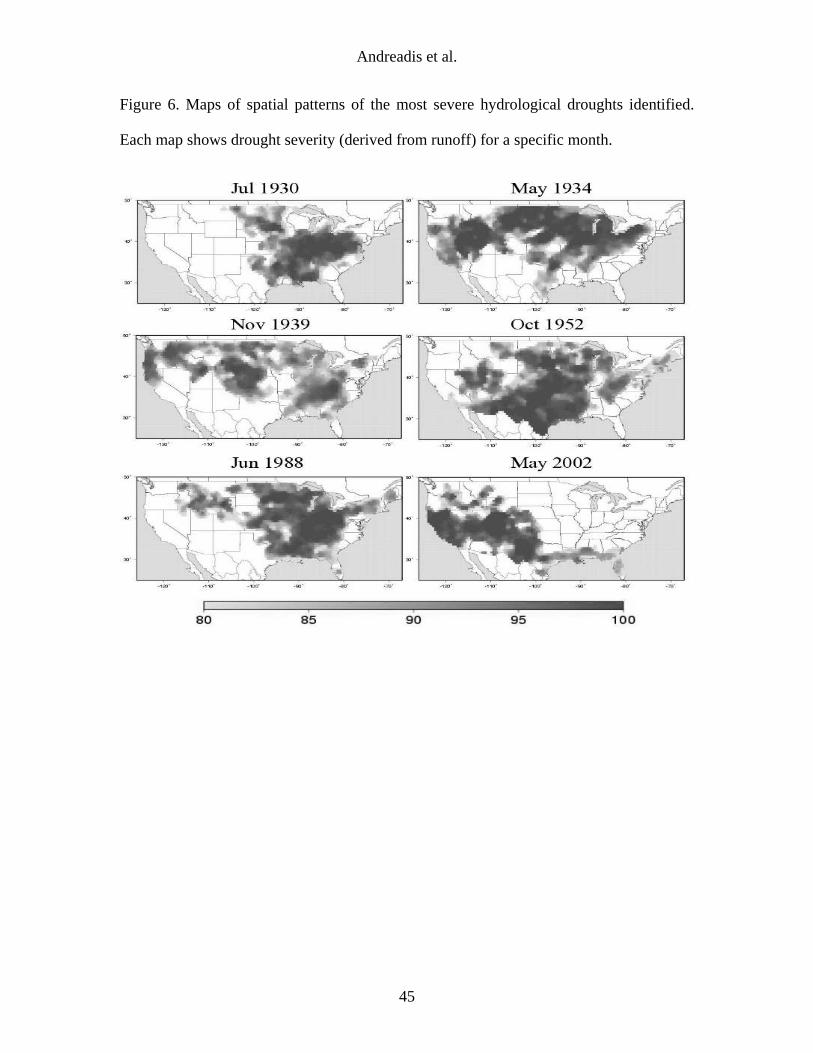
again is identified as a single continuous event. Figure 6 shows spatial maps of each of
the major runoff-derived droughts for a specific month. The displayed month was
selected using the same approach as in Figure 2. The maps show that the ‘Dust Bowl’ had
Andreadis et al.
20
the largest impact, in terms of streamflow, in the mid-1930s. The 1950s drought had a
very large spatial extent covering the Great Plains and reaching southward to Texas and
parts of Colorado. Finally, the 1988 and early 2000s drought spatial patterns agree well
with the ones derived from soil moisture.
The temporal variations of hydrological drought area over the continental U.S.
and areally averaged runoff percentiles are shown in Figure 7. The trends in the time
series of runoff appear similar with the ones from soil moisture. However, the magnitude
of the 1930s and 1950s droughts in terms of runoff appears less pronounced than in the
soil moisture analysis. Another difference with the soil moisture time series is that the
month to month variability is much larger, which is in agreement with the memory
associated with the processes governing soil moisture variability. Nonetheless, the
drought events appearing as the most severe are the same as those identified from soil
moisture.
The envelope curve is rather different than the soil moisture envelope curve.
Figure 8 shows the runoff-based envelope curve for selected durations and area
increments up to 7 million km2. The prominent feature of the curve is that the early
2000s drought occupies a larger portion of the 3- to 24-month curves than in the soil
moisture analysis. As we can see in the accompanying spatial maps, the early 2000s
drought effectively covers the entire western U.S., and is the most severe drought of
record for durations up to 2 years. This suggests that there were minimal recovery periods
for the entire region, amplifying its severity. The 1930s drought stands out as the most
severe drought for the mid to larger spatial extents with decreasing frequency from the 3-
month to the 1-year duration curves. The 1950s drought is the most severe event for the
largest spatial extents and longest duration curves. In fact, it is always the most severe
Andreadis et al.
21
drought for areas larger than 2.5 million km2 (30% of the continental U.S.) and for 24-,
48-month durations. Moreover, the 72-month envelope curve is occupied exclusively by
the 1950s drought. For the smallest areas the 1975-1978 drought in the Great Lakes
region occupies the leftmost part of the 3-month curve.
Figure 9 shows the SAD curves for these events for durations of 3, 12, 24, and 48
months. In the 3-month curves (Figure 9a) the 1932-1938, 1975-1978 and 1999-2003
droughts plot close for small to mid-size areas, with the latter two events displaying an
expected decrease in severity for larger areas where the 1930s drought dominates. In
Figure 9b (12-month duration) the early 2000s drought dominates for areas up to 3
million km2, with the 1950s drought having a similar (and eventually larger) severity as
area increases. The 1932-1938 drought appears as the last point on the envelope curve,
but had a much smaller relative severity for smaller areas. This is also the case for the
other 1930s drought (1928-1932), which has a convex shape. This is an effect of the SAD
technique; that is, the contiguity constraint forces the algorithm to search for the largest
severity pixels in the neighborhood of the area already computed. Therefore, for some of
the smaller areas the average severity is smaller than the average severity of the larger
areas. In the 24-month SAD curves (Figure 9c), the early 2000s drought is clearly the
dominant for small spatial extents, but for mid to larger areas the 1950s drought occupies
the envelope curve, although it has a similar severity to the 1930s drought events. The
48-month SAD curves (Figure 9d) show that the 1950s drought is the most severe
drought with the exception of the very small areas that show the early 2000s drought as
the one having the largest severity.

Andreadis et al.
22
8. Discussion
Table 1 lists the major droughts in the 20th century as identified in the literature
using a variety of methods. In this section we evaluate our results in comparison with the
other studies summarized in Table 1. All of the events shown in Table 1 were also
identified in our analysis. An interesting comparison can be made with the results from
Cook et al. (1999), who used tree-ring chronologies to reconstruct U.S. droughts from
1700-1978 using monthly PDSI. They then used principal components analysis to
identify climate regions and then examined the average signal over the U.S. for severe
drought events. They found that the 1930s "Dust Bowl" was the most severe drought in
the continental U.S. during their period of analysis (1700-1978). They also found that the
3rd most severe drought occurred in 1977, which qualitatively agrees with our results
which show that the mid to late 70s drought is the most severe hydrological drought for
small spatial extents. Although the 1950s drought was found as a notable drought event
by Cook et al., it did not have the same magnitude as shown in our analysis.
Nevertheless, in terms of the temporal resolution of the Cook et al. study (monthly) our
results seem to be in accordance, in particular our finding that the 1930s was the most
intense drought period (high severity for short durations) on average in the U.S.
Conceptually, the sequence of drought types begins with meteorological drought
and as its duration increases, agricultural (soil moisture) drought and hydrologic
(streamflow) drought follow. Simplistically, one would expect that the most severe
droughts for runoff should be about the same as for soil moisture, especially taking into
account the time scales of our analysis. However, our results showed that although the
early 2000s drought had a relatively high soil moisture-based severity, it occupied a much
larger portion of the runoff-based envelope curve. It is worth exploring the causes of this
Andreadis et al.
23
difference, especially when taking into account the socioeconomic importance of the
early 2000s western U.S. drought.
The SAD curves are constructed based on average cumulative severity of different
areas that are experiencing drought over a given duration. Runoff is affected by soil
moisture deficits; if we examine the spatially averaged correlation coefficient between
soil moisture and runoff for the periods of the three major drought events (1930s, 1950s
and early 2000s), we find that the correlation is much higher for the early 2000s drought
(Table 2). A possible explanation might be inferred from the correlations between soil
moisture and runoff with precipitation, in the context of drought recovery. Table 2 shows
the correlations between the spatially averaged (over the western U.S.) soil moisture,
runoff and precipitation percentiles. Precipitation has a much higher correlation with
runoff than with soil moisture. This follows from the fact that soil moisture is relatively
more persistent than runoff, and that the latter responds more quickly to precipitation
signals. The early 2000s hydrological drought is more severe (when compared to the
relative position of the respective agricultural drought on the SAD envelope curve)
mainly for the 6- and 12-month durations and for areas that occupy the middle part of the
curves. Figure 10 shows the autocorrelation of the spatially averaged monthly
precipitation for the three drought events and lags from 1 to 12 months. The
autocorrelation is significantly higher for the early 2000s drought, which suggests that
dry (or wet) spells during that drought event were longer than during the other two
droughts. Because runoff responds faster to precipitation, parts of the areas under
hydrological drought in the 1930s and 1950s recovered, thus decreasing the average
severity.

Andreadis et al.
24
The above discussion simply describes the processes that drive drought events of
large magnitude. An increasing number of studies have looked at the relationship
between extreme droughts and climate teleconnections, such as the El Nino Southern
Oscillation (ENSO) and Pacific Decadal Oscillation (PDO) (e.g. Trenberth et al. 1988;
Schubert et al. 2004). A simple correlation analysis between the VIC simulated end-of-
summer soil moisture and runoff, and January SST anomalies (not shown here) exhibits
strong correlations in the northwestern and southwestern U.S., as expected. However, a
similar analysis of end-of-summer soil moisture and runoff for individual persistent
severe drought events did not display any characteristic spatial structure, suggesting that
a more complicated climate signal is associated with these extreme droughts (Hoerling
and Kumar 2003).
9. Summary and Conclusions
Retrospective simulations of soil moisture and runoff across the continental U.S.
were performed for the period 1920-2003. An empirical probability distribution was fit to
these data to produce percentiles corresponding to the monthly soil moisture and runoff
for each half degree grid cell. Contiguous grid cells experiencing lower than 20th
percentile soil moisture, or streamflow, at each monthly timestep were considered to
constitute drought events. These events were then reclassified based on their temporal
continuity. Grid cells included in the final drought classification were then input to a
scheme termed Severity-Area-Duration analysis, which represents the relationship
between these drought characteristics for each drought event. Envelope curves for each
drought duration were then produced, representing the most severe drought events in the
study period over the study domain.

Andreadis et al.
25
Drought severity calculated using the simulated soil moisture and runoff
percentiles is limited by errors and biases inherent in the model physics, parameters, and
forcing data. Nonetheless, validation of VIC soil moisture and streamflow predictions in
different regions of the U.S., and the identification of drought events that have already
been cited as extreme droughts in the 20th century, support our use of an approach based
on soil moisture and runoff derived from VIC model simulations. The model products
provide a spatially and temporally continuous dataset of hydrologic variables, which are
estimated using a physically based model that accounts for various land surface processes
(such as cold land processes), in contrast with other drought indices that employ simple
water balance models. The technique presented in this paper employs a physically-based
criterion for drought identification that is applicable across climate regions. Since many
of the most severe droughts in the U.S. cross climate region boundaries, regionalization
that other studies have employed limits the maximum spatial component of drought
impacts – a limitation that our method avoids. Whereas many studies produce time-series
of regional drought evolution, SAD analysis directly characterizes specific drought
events, both spatially and temporally. SAD is thus meant to be a supplementary tool in
drought characterization.
The primary features of the evolution of 20th century U.S. droughts, as reflected in
the constructed SAD and envelope curves, can be summarized as follows:
• The drought events of the 1930s and 1950s were the most severe
experienced in the (last 80 years of the) 20th century for large areas.
However, in our analysis the 1930s “Dust Bowl” was the most intense
drought (largest severity for short durations), a conclusion that agrees with
previous studies that examined drought severity over short timescales. On

Andreadis et al.
26
the other hand, the 1950s drought was the most persistent event, having
the largest severity for long durations.
• The early 2000s drought in the western U.S. is among the most severe in
the period of record, especially when averaged over small areas and short
durations. Since the early 2000s drought is still developing, it is possible
that it may appear among the most severe droughts at longer durations.
• In general, the most severe agricultural droughts (defined by simulated
soil-moisture) were also among the most severe hydrologic droughts
(defined by simulated runoff). The early 2000s drought, however,
occupies a larger portion of the hydrologic drought envelope curve than
does its agricultural companion.
• Runoff tends to recover in response to precipitation more quickly than soil
moisture, so the severity of hydrologic drought during the 1930s and
1950s was dampened by short wet spells while the severity of the early
2000s drought remained high due to the relative absence of these short
term phenomena.
In theory, SAD curves can be treated similarly to DAD curves, in terms of water
management. The primary purpose of this type of characterization is to provide a
historical perspective when planning for future drought mitigation. However, because of
model uncertainty, this technique should only be used in conjunction with existing
drought planning tools. SAD could also be applied in the context of climate change
analysis to assess whether climate trends are changing (or have the potential to alter) the
severity of drought occurrence. An interesting application of this technique would be the
coupling of a General Circulation Model (GCM) with a land surface scheme (e.g. VIC) to

Andreadis et al.
27
provide the input dataset to the SAD technique. In a hydrologic forecasting context,
ensemble techniques could be incorporated and corresponding probabilities of drought
occurrence can be estimated. Future studies may include real-time applications of this
technique across the continental U.S. with an emphasis on the probability of recovery.

Andreadis et al.
28
References
Alley, W.M., 1984: The Palmer Drought Severity Index: limitations and assumptions. J.
Clim. Appl. Met., 23, 1100-1109.
Atlas, R., N. Wolfson, and J. Terry, 1993: The effect of SST and soil moisture anomalies
on GLA model simulations of the 1988 U.S. summer drought. J. Climate, 6, 2034-
2048.
Climate Prediction Center, 2005: U.S. Soil Moisture Monitoring.
http://www.cpc.ncep.noaa.gov/soilmst/.
Cook, E.R., and G.C. Jacoby Jr., 1977: Tree-ring-drought relationships in the Hudson
Valley, New York. Science, 198, 399-401.
Cook, E.R., D.M. Meko, D.W. Stahle, and M.K. Cleaveland, 1999: Drought
reconstructions for the continental United States. J. Climate, 12, 1145-1162.
Dai, A., K.E. Trenberth, and T.R. Karl, 1998: Global Variations in Droughts and Wet
Spells, Geophys. Res. Lett., 25, 3367-3370.
Dai, A., K.E. Trenberth, and T. Qian, 2004: A global data set of Palmer Drought Severity
Index for 1870-2002: relationship with soil moisture and effects of surface warming.
J. Hydrometeor., 5, 1117-1130.
Dalezios, N.R., A. Loukas, L. Vasiliades, and E. Liakopoulos, Severity-Duration-
Frequency Analysis of Droughts and Wet Periods in Greece, Hydrol. Scienc., 45,
751-769.
Daly, C., R.P. Neilson, D.L. Phillips, 1994: A statistical-topographic model for mapping
climatological precipitation over mountainous terrain. J. Appl. Meteor., 33, 140-158.

Andreadis et al.
29
Dhar, O.N., and S. Nandargi, 1993: Envelope depth-area-duration rain depths for
different homogeneous rainstorm zones of the Indian region. Theoret. and Appl.
Climatology, 47, 117-125.
Dracup, J.A., K.S. Lee, and E.G. Paulson, Jr., 1980a: On the definition of droughts.
Water Resour. Res., 16, 297-302.
Dracup, J.A., K.S. Lee, and E.G. Paulson, Jr., 1980b: On the statistical characteristics of
drought events. Water Resour. Res., 16, 289-296.
Felch, R.E., 1978: Drought: characteristics and assessment. North American Droughts,
N.J. Rosenberg, ed., Amer. Assoc. Adv. Sci. Selected Symp., vol. 15, Westview
Press, 25-42.
Grebner, D., and T. Roesch, 1997: Regional dependence and application of DAD
relationships, FRIEND '97--Regional Hydrology: Concepts and Models for
Sustainable Water Resource Management (Proceedings of the Postojna, Slovenia,
Conference, September-October 1997), eds. A.Gustard, S. Blazkova, M. Brilly, S.
Demuth, J. Dixon, H. van Lanen, C. Llasat, S. Mkhandi, and E. Servat. IAHS Publ.
no. 246, 223-230.
Hamlet, A.F., and D.P. Lettenmaier, 2005: Production of temporally consistent gridded
precipitation and temperature fields for the continental U.S., J. Hydromet (in press).
Hansen, M.C., R.S. DeFries, J.R.G. Townshend, and R. Sohlberg, 2000: Global land
cover classification at 1 km spatial resolution using a classification tree approach.
Int. J. Remote Sens., 21, 1331-1364.
Hisdal, H., and L.M. Tallaksen, 2003: Estimation of regional meteorological and
hydrological drought characteristics: A case study for Denmark. J. Hydrol., 281, 230-
247.

Andreadis et al.
30
Hoerling, M., and A. Kumar, 2003: The Perfect Ocean for Drought, Science, 299, 691-
694.
Huang, J., H.M. Van den Dool, and K. P. Georgakakos, 1996: Analysis of model
calculated soil moisture over the United States (1931-1993) and applications to long-
range temperature forecasts. J. Climate, 9, 1350-1362.
Karl, T.R., Williams, C.N. Jr., Quinlan F.T., and Boden T.A., 1990: United States
Historical Climatology Network (HCN) serial temperature and precipitation data,
Environmental Science Division Publication No. 3404, Carbon Dioxide Information
and Analysis Center, Oak Ridge National Laboratory, Oak Ridge, TN, 389 pp
Karl, T.R., and A.J. Koscielny, 1982: Drought in the United States: 1895-1981. J. of
Climatol., 2, 313-329.
Karl, T.R., and R. G. Quayle, 1981: The 1980 summer heat wave and drought in
historical perspective. Mon. Wea. Rev., 109, 2055-2073.
Keyantash, J.A., and J.A. Dracup, 2004: An Aggregate Drought Index; Assessing
Drought Severity Based on Fluctuations in the Hydrologic Cycle and Surface Water
Storage. Water Resour. Res., W09304, doi:10.1029/2003WR002610.
Liang, X., D.P. Lettenmaier, E.F. Wood, and S.J. Burges, 1994: A simple hydrologically
based model of land surface water and energy fluxes for GSMs. J. Geophys. Res., 99,
14415-14428.
Liang, X., D.P. Lettenmaier, E.F. Wood, and S.J. Burges, 1996: One-dimensional
statistical dynamic representation of subgrid spatial variability of precipitation in the
two-layer variable infiltration capacity model. J. Geophys. Res., 101, 21403-21422.
Ludlum, D.M., 1982: The American Weather Book. Houghton-Mifflin, 296 pp.

Andreadis et al.
31
Maurer, E.P., A.W. Wood, J.C. Adam, and D.P. Lettenmaier, 2002: A long-term
hydrologically based dataset of land surface fluxes and states for the conterminous
United States. J. Climate, 15, 3237-3251.
Mekis, E. and Hogg W.D., 1999: Rehabilitation and analysis of Canadian daily
precipitation time series. Atmosphere-Ocean, 37, 53-85
National Climatic Data Center (NCDC), 2003: Data Documentation for Data Set 3206
(DSI-3206): Coop Summary of the Day -- CDMP -- Pre 1948. Asheville, NC,
http://www4.ncdc.noaa.gov/ol/documentlibrary/datasets.html
Nicks, A.D., and F.A. Igo, 1980: A depth-area-duration model of storm rainfall in the
Southern Great Plains. Water Resour. Res., 16, 939-945.
Nijssen, B., R. Schnur, and D.P. Lettenmaier, 2001: Global Retrospective Estimation of
Soil Moisture Using the Variable Infiltration Capacity Land Surface Model, 1980-93.
J. Climate, 14, 1790-1808.
Oladipo, E.O., 1986: Spatial patterns of drought in the Interior Plains of North America.
J. of Climatol., 6, 495-513.
Palmer, W.C., 1965: Meteorological Drought, Res. Paper no. 45. U.S. Department of
Commerce, Weather Bureau, 58 pp.
Robock, A., K.Y. Vinnikov, G. Srinivasan, J.K. Entin, S.E. Hollinger, N.A. Speranskaya,
S. Liu, and A. Namkhai, 2000: The Global Soil Moisture Data Bank. Bull. Amer.
Meteor. Soc., 81, 1281-1299.
Robock, A., et al., 2003: Evaluation of the North American Land Data Assimilation
System Over the Southern Great Plains During the Warm Season. J. Geophys. Res.,
108(D22), 8846, doi:10.1029/2002JD003245.

Andreadis et al.
32
Sheffield, J., G. Goteti, F. Wen, and E.F. Wood, 2004: A simulated soil moisture based
drought analysis for the USA. J. Geophys. Res., 109, D24108, doi:
10.1029/2004JD005182..
Schubert, S.D., M.J. Suarez, P.J. Pegion, R.D. Koster, and J.T. Bacmeister, 2004: On the
cause of the 1930s Dust Bowl. Science, 303, 1855-1859.
Soulé, P.R., 1993: Hydrologic drought in the contiguous United States, 1900-1989:
spatial patterns and multiple comparison of means. Geophys. Res. Letters, 20, 2367-
2370.
Trenberth, K.E., G.W. Branstator., and P.A. Arkin, 1988: Origins of the 1988 North
American drought. Science, 242, 1640-1645.
U.S. Drought Monitor, 2003: Drought monitor: state-of-the-art blend of science and
subjectivity, National Drought Mitigation Center.
http://drought.unl.edu/dm/archive/99/classify.htm.
Vincent L.A., and Gullett D.W., 1999: Canadian historical and homogeneous
temperature datasets for climate change analyses, International Journal of
Climatology, 19, 1375-1388
Webb, R.H., G.J. McCabe, R. Hereford, and C. Wilkowske, 2004: Climate fluctuations,
drought, and flow in the Colorado River. USGS Fact Sheet 3062-04.
Wilhite, D.A. and M.H. Glantz, 1985: Understanding the drought phenomenon: The role
of definitions, Water Int’l, 10, 111-120.
Willeke, G., J.R.M. Hosking, J.R. Wallis, and N.B. Guttman, 1994: The National
Drought Atlas. IWR Report 94-NDS-4, 587 pp.

Andreadis et al.
33
World Meteorological Organization (WMO), 1969: Manual for Depth-Area-Duration
Analysis of Storm Precipitation, WMO (Series): no. 237.TP.129. Secretariat of
WMO, 114 pp.

Andreadis et al.
34
List of Tables
Table 1. Notable 20th century droughts in the conterminous United States
Table 2. Correlations between spatially averaged (over the western U.S.) precipitation,
soil moisture, runoff percentiles for three different drought events (1930s, 1950s, and
early 2000s)

Andreadis et al.
35
List of Figures
Figure 1. Spatiotemporal drought identification: three consecutive timesteps, with two
drought areas merging (A1 and A2); drought area B2 breaking up into two drought areas,
B2 and B3, with the latter merging with another drought area (B1). The algorithm
classifies each smaller drought area to a larger drought event (A and B).
Figure 2. Maps of spatial patterns of the most severe agricultural droughts identified.
Each map shows drought severity (derived from soil moisture) for a specific month.
Figure 3. Monthly time series of percent area characterized as agricultural drought, and
spatially averaged drought severity (derived from soil moisture). The subplots correspond
to the entire, western, central, and eastern U.S. respectively.
Figure 4. SAD envelope curves based on soil moisture. Each curve corresponds to a
specific drought duration (3, 6, 12, 24, 48 and 72 months). Different colors correspond to
the drought events from which the specific point was derived.
Figure 5. SAD curves for the major drought events identified from soil moisture. Each
subplot corresponds to different analysis duration: (a) 3 months, (b) 12 months, (c) 24
months, and (d) 48 months.
Figure 6. Maps of spatial patterns of the most severe hydrological droughts identified.
Each map shows drought severity (derived from runoff) for a specific month.

Andreadis et al.
36
Figure 7. Monthly time series of percent area characterized as hydrological drought, and
spatially averaged drought severity (derived from runoff). The subplots correspond to the
entire, western, central, and eastern U.S. respectively.
Figure 8. SAD envelope curves based on runoff. Each curve corresponds to a specific
drought duration (3, 6, 12, 24, 48 and 72 months). Different colors correspond to the
drought events from which the specific point was derived.
Figure 9. SAD curves for the major drought events identified from runoff. Each subplot
corresponds to different analysis duration: (a) 3 months, (b) 12 months, (c) 24 months,
and (d) 48 months.
Figure 10. Autocorrelation coefficient of the spatially averaged (over the western U.S.)
precipitation for three different periods corresponding to three drought events (1930s,
1950s, and 2000s). Values of the autocorrelation coefficient up to a lag of 12 months are
shown.

Andreadis et al.
37
Table 1. Notable 20th century droughts in the conterminous U.S.
Dates Location Type of Data Sources
1910-
1913
Western Kansas PDSI Palmer (1965); Ludlum (1982)
1931-
1940
Great Plains eastward to
Great Lakes, southwestern
U.S.
Precipitation,
temperature;
Reconstructed
PDSI
Schubert et al. (2004); Cook et al.
(1999); Weakly (1965), as cited in
Bark (1978); Ludlum (1982)
1947 Central Iowa PDSI Palmer (1965)
Mid-
1950s
Great Plains to southeastern
U.S.
Reconstructed
PDSI
Cook et al. (1999); WWB, Stahl
and Cleaveland (1988); Palmer
(1965); Weakly (1965), as cited in
Bark (1978); Ludlum (1982); Karl
and Quayle (1981)
1961-
1966
Northeastern U.S., North
Dakota
PDSI,
reconstructed
PDSI
Cook and Jacoby (1977); Cook et
al. (1999); Palmer (1965); Ludlum
(1982)
Mid-
1970s
Western U.S. PDSI, Aggregate
Drought Index
Felch (1978); Webb et al. (2004),
citing NOAA (2004); Ludlum
(1982); Keyantash and Dracup
(2004)

Andreadis et al.
38
Dates Location Type of Data Sources
1980-
1981
Southern and southeastern
U.S.
PDSI, Z-index,
population-
weighted cooling
degree days as
related to
electrical energy
sales
Karl and Quayle (1981)
1987-
1988
West coast, northwestern
U.S., north central U.S., Great
Plains, Utah
Precipitation,
PDSI, Aggregate
Drought Index
Trenberth et al. (1988); Webb et al.
(2004), citing NOAA (2004); Atlas
et al. (1993); Keyantash and Dracup
(2004)
1996 Utah PDSI Webb et al. (2004); citing NOAA
(2004)

Andreadis et al.
39
Table 2. Correlations between spatially averaged (over the western U.S.) precipitation,
soil moisture, runoff percentiles for three different drought events (1930s, 1950s, and
2000s).
Correlation Coefficient R2
Drought
Event Runoff-Soil
Moisture
Precipitation-
Runoff
Precipitation-Soil
Moisture
1930s 0.686 0.655 0.232
1950s 0.766 0.759 0.357
2000s 0.922 0.799 0.570
Andreadis et al.
40
Figure 1. Spatiotemporal drought identification: three consecutive timesteps, with two
drought areas merging (A1 and A2); drought area B2 breaking up into two drought areas,
B2 and B3, with the latter merging with another drought area (B1). The algorithm
classifies each smaller drought area to a larger drought event (A and B).

Andreadis et al.
41
Figure 2. Maps of spatial patterns of the most severe agricultural droughts identified.
Each map shows drought severity (derived from soil moisture) for a specific month.

Andreadis et al.
42
Figure 3. Monthly time series of percent area characterized as agricultural drought (solid
line), and spatially averaged drought severity (derived from soil moisture; dotted line).
The subplots correspond to the entire, western, central, and eastern U.S. respectively.

Andreadis et al.
43
Figure 4. SAD envelope curves based on soil moisture. Each curve corresponds to a
specific drought duration (3, 6, 12, 24, 48 and 72 months). Different colors correspond to
the drought events from which the specific point was derived.

Andreadis et al.
44
Figure 5. SAD curves for the major drought events identified from soil moisture. Each
subplot corresponds to different analysis duration: (a) 3 months, (b) 12 months, (c) 24
months, and (d) 48 months.
(a) 3 Month Duration (b) 12 Month Duration
(c) 24 Month Duration (d) 48 Month Duration
Andreadis et al.
45
Figure 6. Maps of spatial patterns of the most severe hydrological droughts identified.
Each map shows drought severity (derived from runoff) for a specific month.

Andreadis et al.
46
Figure 7. Monthly time series of percent area characterized as hydrological drought (solid
line), and spatially averaged drought severity (derived from runoff; dotted line). The
subplots correspond to the entire, western, central, and eastern U.S. respectively.

Andreadis et al.
47
Figure 8. SAD envelope curves based on runoff. Each curve corresponds to a specific
drought duration (3, 6, 12, 24, 48 and 72 months). Different colors correspond to the
drought events from which the specific point was derived.

Andreadis et al.
48
Figure 9. SAD curves for the major drought events identified from runoff. Each subplot
corresponds to different analysis duration: (a) 3 months, (b) 12 months, (c) 24 months,
and (d) 48 months.
(a) 3 Month Duration (b) 12 Month Duration
(c) 24 Month Duration (d) 48 Month Duration

Andreadis et al.
49
Figure 10. Autocorrelation coefficient of the spatially averaged (over the western U.S.)
precipitation for three different periods corresponding to three drought events (1930s,
1950s, and 2000s). Values of the autocorrelation coefficient up to a lag of 12 months are
shown.