2

Outline

• Introduction– Motivation and Goals– Grayscale Chromosome Images– Multi-spectral Chromosome Images

• Contributions

• Results

• Conclusions

3

Motivation and Goals

• Chromosomes store genetic information• Chromosome images can indicate genetic disease,

cancer, radiation damage, etc.• 325 clinical cytogenetic US labs perform over

250,000 diagnostic studies per year involving chromosome analysis

• Research goals:– Locate and classify each chromosome in an image– Locate chromosome abnormalities

4

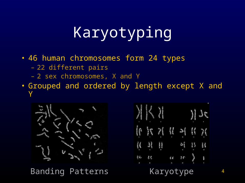
Karyotyping

• 46 human chromosomes form 24 types– 22 different pairs– 2 sex chromosomes, X and Y

• Grouped and ordered by length except X and Y

Banding Patterns Karyotype

5

Chromosome Abnormalities

• Abnormal number– Turner’s Syndrome (1 X, no Y chromosome)– Down’s Syndrome (3 of type 21)

• Translocations: Chronic myelogenous leukemia (type 9 and type 22)

• Deletions of genetic material: William’s Syndrome (gene missing in type 7)

• Research goals:– Locate and classify each chromosome in an image– Locate chromosome abnormalities

6

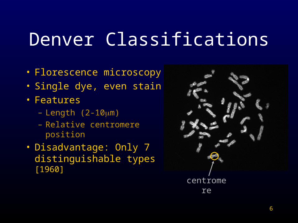
Denver Classifications

• Florescence microscopy• Single dye, even stain• Features

– Length (2-10m)

– Relative centromereposition

• Disadvantage: Only 7 distinguishable types [1960]

centromere

7

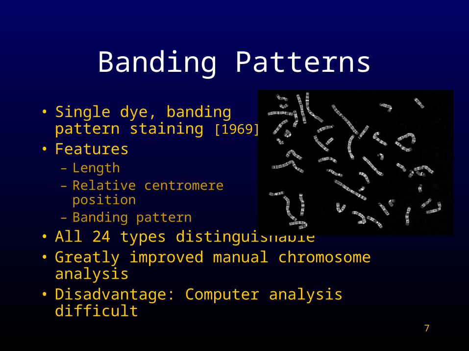
Banding Patterns

• Single dye, bandingpattern staining [1969]

• Features– Length– Relative centromere

position– Banding pattern

• All 24 types distinguishable• Greatly improved manual chromosome analysis• Disadvantage: Computer analysis difficult

8

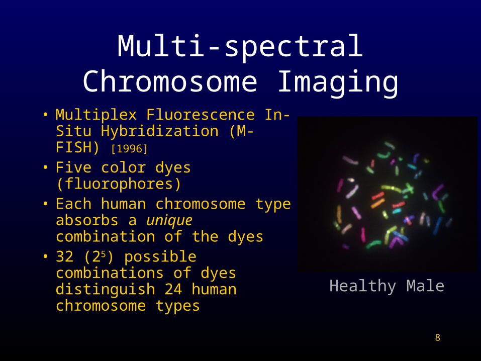
Multi-spectral Chromosome Imaging

• Multiplex Fluorescence In-Situ Hybridization (M-FISH) [1996]

• Five color dyes (fluorophores)• Each human chromosome type

absorbs a unique combination of the dyes

• 32 (25) possible combinations of dyes distinguish 24 human chromosome types

Healthy Male

9

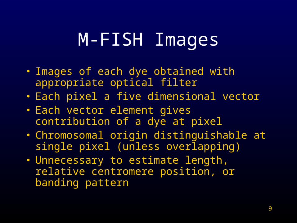
M-FISH Images

• Images of each dye obtained with appropriate optical filter

• Each pixel a five dimensional vector• Each vector element gives contribution of a dye

at pixel• Chromosomal origin distinguishable at single

pixel (unless overlapping)• Unnecessary to estimate length, relative

centromere position, or banding pattern

10

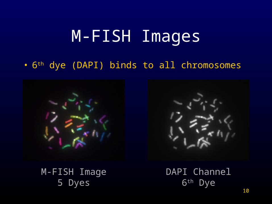
M-FISH Images

• 6th dye (DAPI) binds to all chromosomes

DAPI Channel6th Dye

M-FISH Image5 Dyes

11

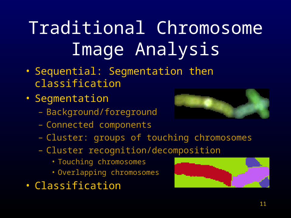
Traditional Chromosome Image Analysis

• Sequential: Segmentation then classification• Segmentation

– Background/foreground

– Connected components

– Cluster: groups of touching chromosomes

– Cluster recognition/decomposition• Touching chromosomes

• Overlapping chromosomes

• Classification

12

Boundary

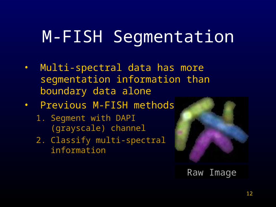
M-FISH Segmentation

• Multi-spectral data has more segmentation information than boundary data alone

• Previous M-FISH methods1. Segment with DAPI

(grayscale) channel

2. Classify multi-spectralinformation

Raw Image

13

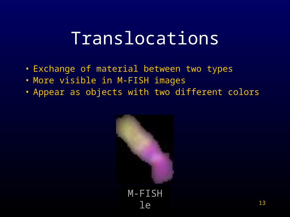
Translocations

• Exchange of material between two types• More visible in M-FISH images• Appear as objects with two different colors

Grayscale

M-FISH

14

Outline

• Introduction• Contributions

1. Chromosome segmentation using multi-spectral information

2. Joint segmentation and classification3. Aberration scoring

• Results • Conclusions

15

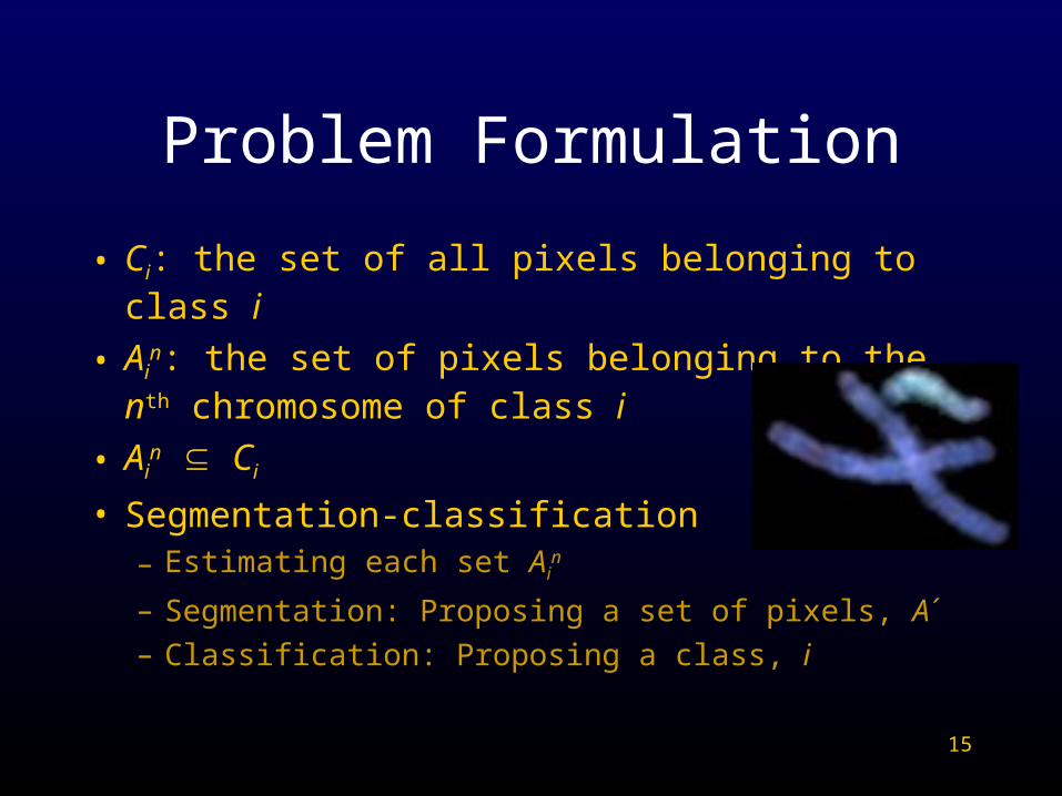
Problem Formulation

• Ci: the set of all pixels belonging to class i

• Ain: the set of pixels belonging to the nth chromosome of class i

• Ain Ci• Segmentation-classification

– Estimating each set Ain

– Segmentation: Proposing a set of pixels, A´

– Classification: Proposing a class, i

16

Proposed Approach

• Develop a measure of quality for segmentation-classification possibilities– Must be a function of both segmentation and

classification

– Measure is also a likelihood

• Choose a reasonable set of segmentation-classification possibilities

• Maximize the measure over the set of possibilities

17

Maximum Likelihood Formulation

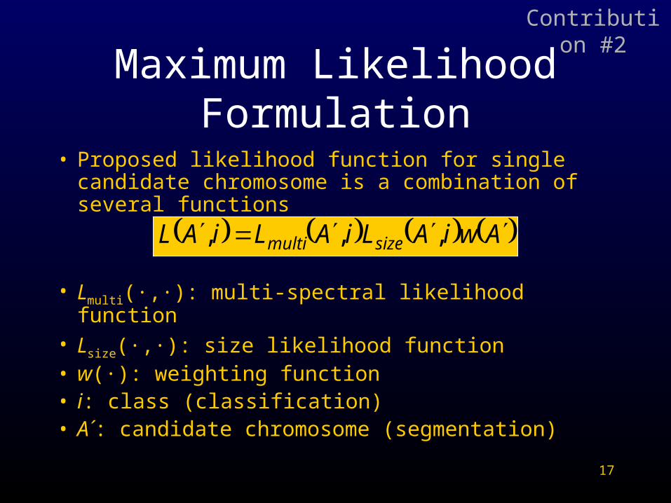
• Proposed likelihood function for single candidate chromosome is a combination of several functions

• Lmulti(·,·): multi-spectral likelihood function• Lsize(·,·): size likelihood function• w(·): weighting function• i: class (classification)• A´: candidate chromosome (segmentation)

AwiALiALiAL sizemulti ,,,

Contribution #2

18

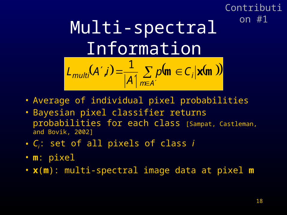
Multi-spectral Information

• Average of individual pixel probabilities• Bayesian pixel classifier returns probabilities for

each class [Sampat, Castleman, and Bovik, 2002]

• Ci: set of all pixels of class i

• m: pixel• x(m): multi-spectral image data at pixel m

Am

imulti CpA

iAL mxm1

,

Contribution #1

19

Size Information

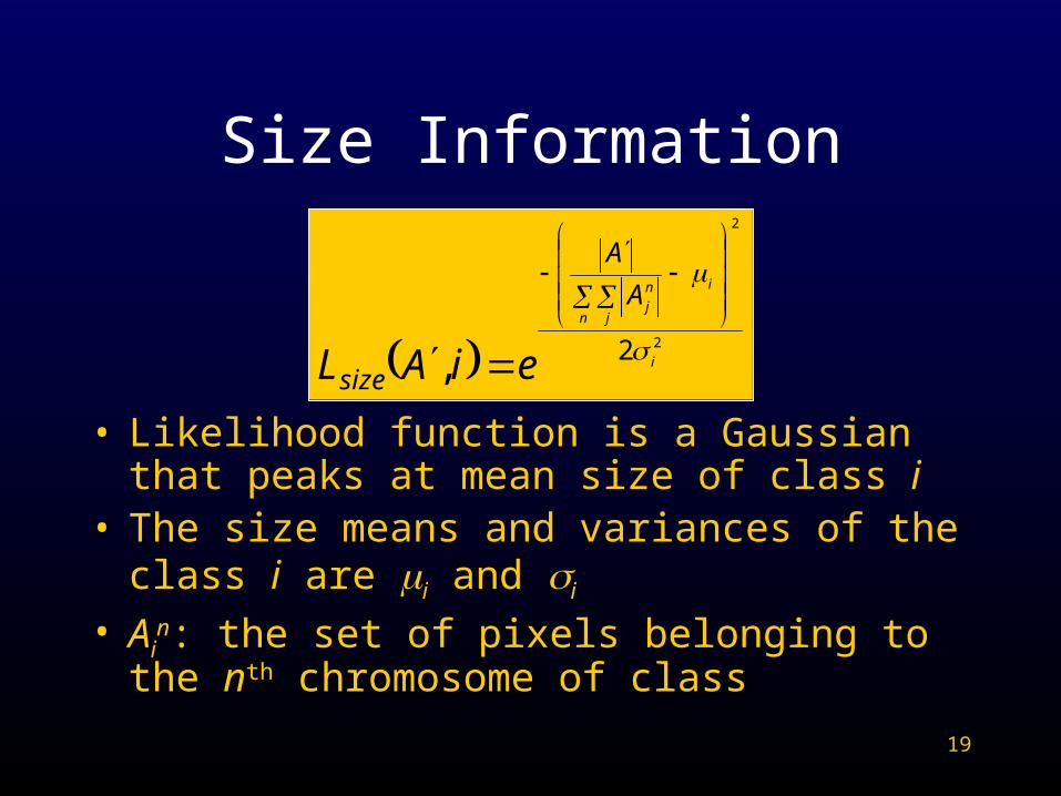
• Likelihood function is a Gaussian that peaks at mean size of class i

• The size means and variances of the class i are i and i

• Ain: the set of pixels belonging to the nth chromosome of class

2

2

2, i

i

n j

n

jA

A

size eiAL

20

Weighting Function

• Measures the certainty of the likelihoods• w(·) is the percentage of visible, or non-

overlapped, pixels in the candidate chromosome • Forces more certain non-overlapped chromosomes

segments to be combined first• Precludes possibility of a segment being left out of

the middle of a chromosome

21

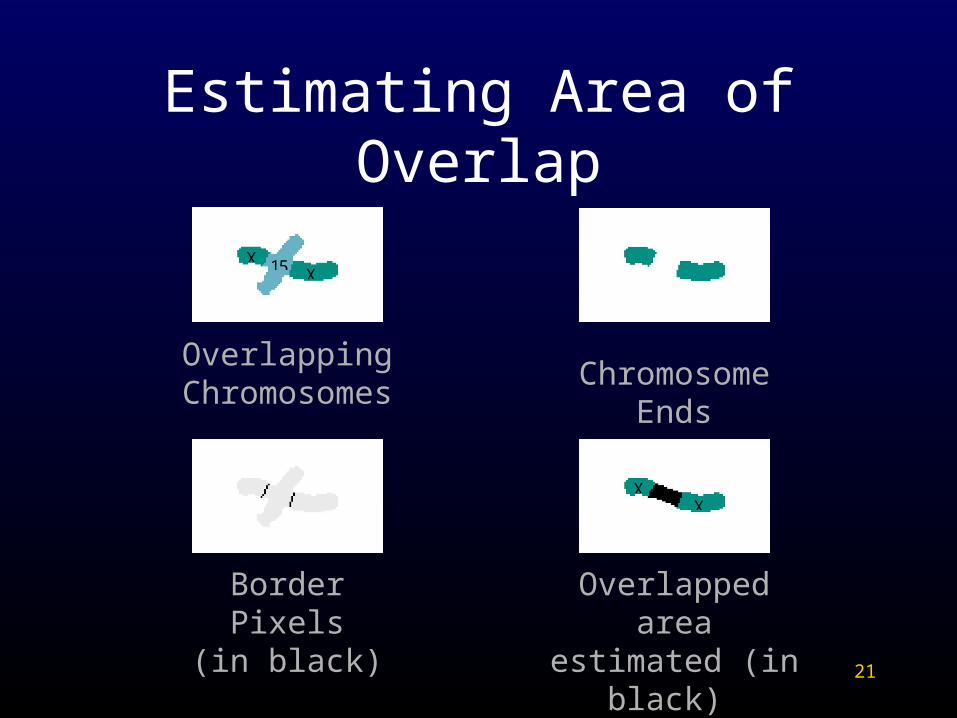
Estimating Area of Overlap

Overlapping Chromosomes

15 X X

Chromosome Ends

Border Pixels(in black)

X X

Overlapped area estimated (in black)

22

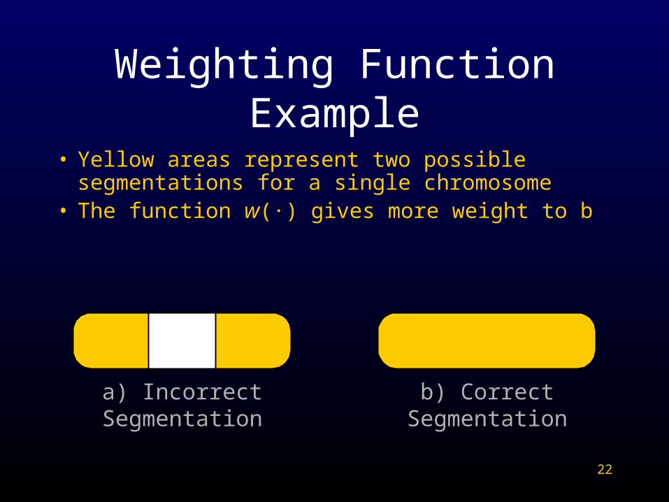
Weighting Function Example

• Yellow areas represent two possible segmentations for a single chromosome

• The function w(·) gives more weight to b

a) Incorrect Segmentation

b) Correct Segmentation

23

Segmentation Implementation

• Use multi-spectral information to determine segmentation possibilities

• Strategy: Oversegment and merge segments– Use pixel classification and post-processing to

determine initial segments

– Merge segments as long as the merging increases the proposed likelihood function

24

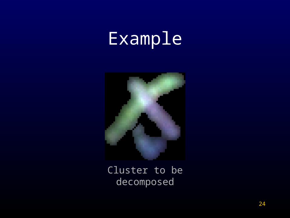
Example

Cluster to be decomposed

25

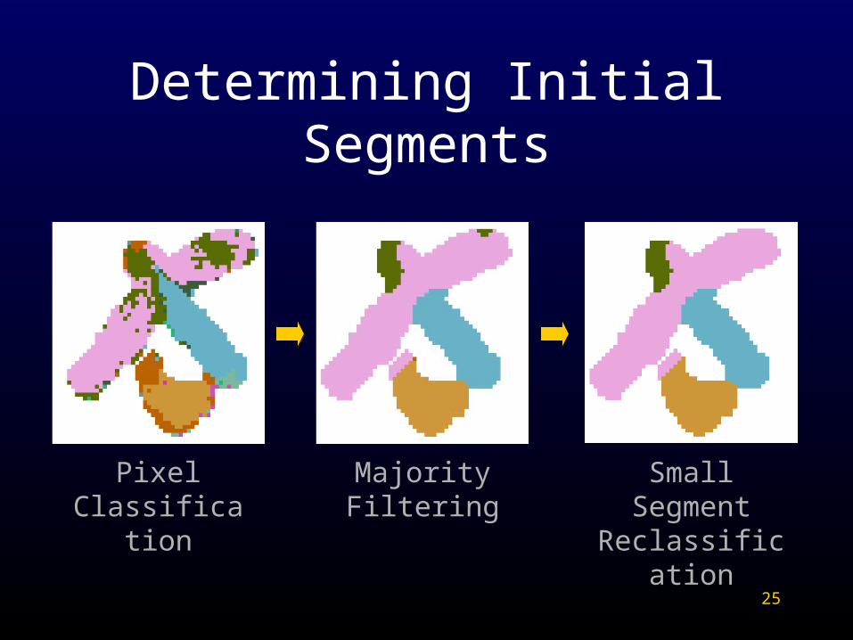
Determining Initial Segments

Pixel Classification

Majority Filtering

Small Segment Reclassification

26

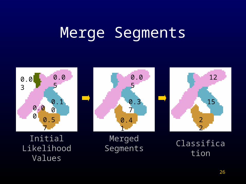
Merge Segments

0.37

0.05

0.41

Merged Segments

0.03 0.05

0.00

0.57

0.10

Initial Likelihood Values

12

15

22

Classification

27

Aberration Scoring

• Aberration scoring: assigning a value to the likelihood of abnormality

• Design of likelihood function has allowed for straightforward aberration scoring– Segments with low likelihood can be flagged as likely

abnormalities– Low likelihood values also identify incorrect

segmentation and classification– Likelihood values help direct user

Contribution #3

28

Outline

• Introduction

• Contributions

• Results– Segmentation– Classification– Aberration Scoring

• Conclusions

29

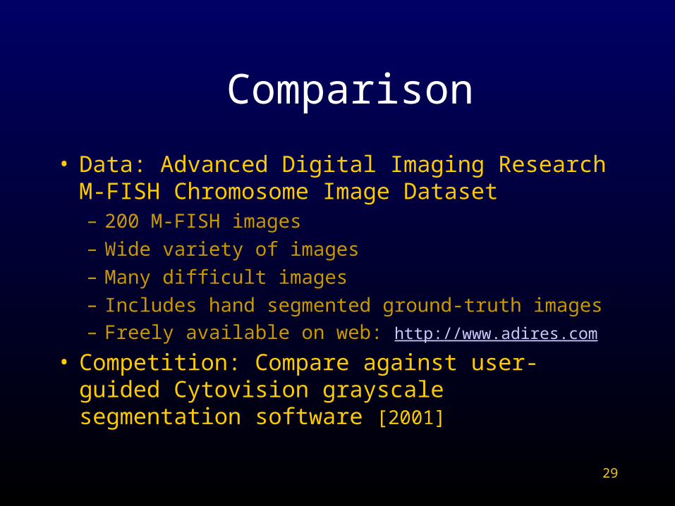
Comparison

• Data: Advanced Digital Imaging ResearchM-FISH Chromosome Image Dataset– 200 M-FISH images

– Wide variety of images

– Many difficult images

– Includes hand segmented ground-truth images– Freely available on web: http://www.adires.com

• Competition: Compare against user-guided Cytovision grayscale segmentation software [2001]

30

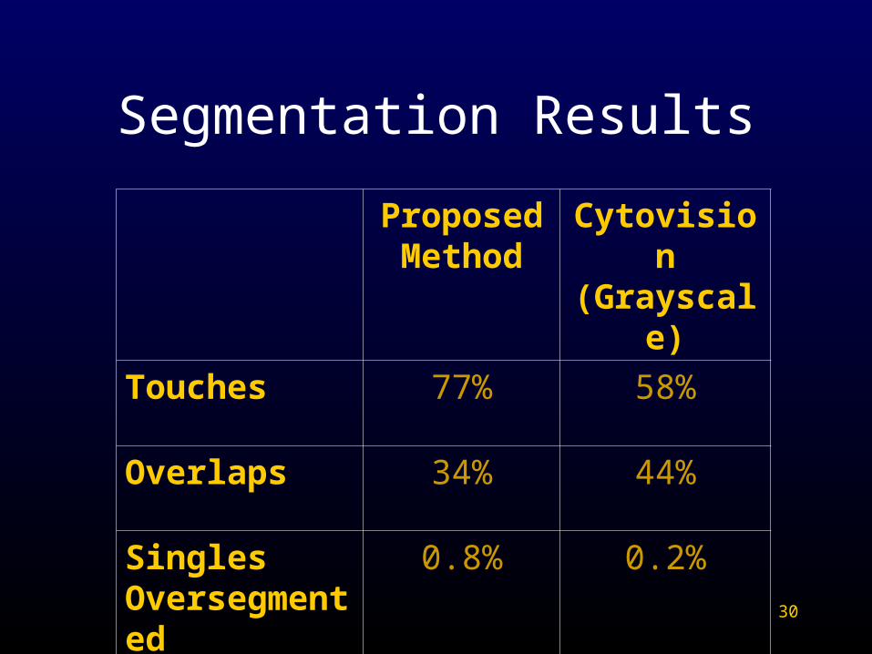
Segmentation Results

Proposed Method

Cytovision(Grayscale)

Touches 77% 58%

Overlaps 34% 44%

Singles Oversegmented

0.8% 0.2%

31

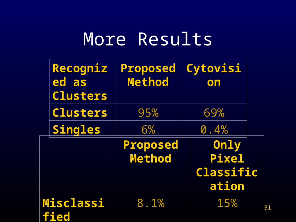
More Results

Recognized as Clusters

Proposed Method

Cytovision

Clusters 95% 69%

Singles 6% 0.4%

Proposed Method

Only Pixel Classification

Misclassified 8.1% 15%

32

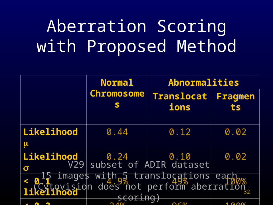
Aberration Scoring with Proposed Method

Normal Chromosomes

Abnormalities

Translocations Fragments

Likelihood 0.44 0.12 0.02

Likelihood 0.24 0.10 0.02

< 0.1 likelihood 4.9% 49% 100%

< 0.3 likelihood 34% 96% 100%V29 subset of ADIR dataset15 images with 5 translocations each

(Cytovision does not perform aberration scoring)

33

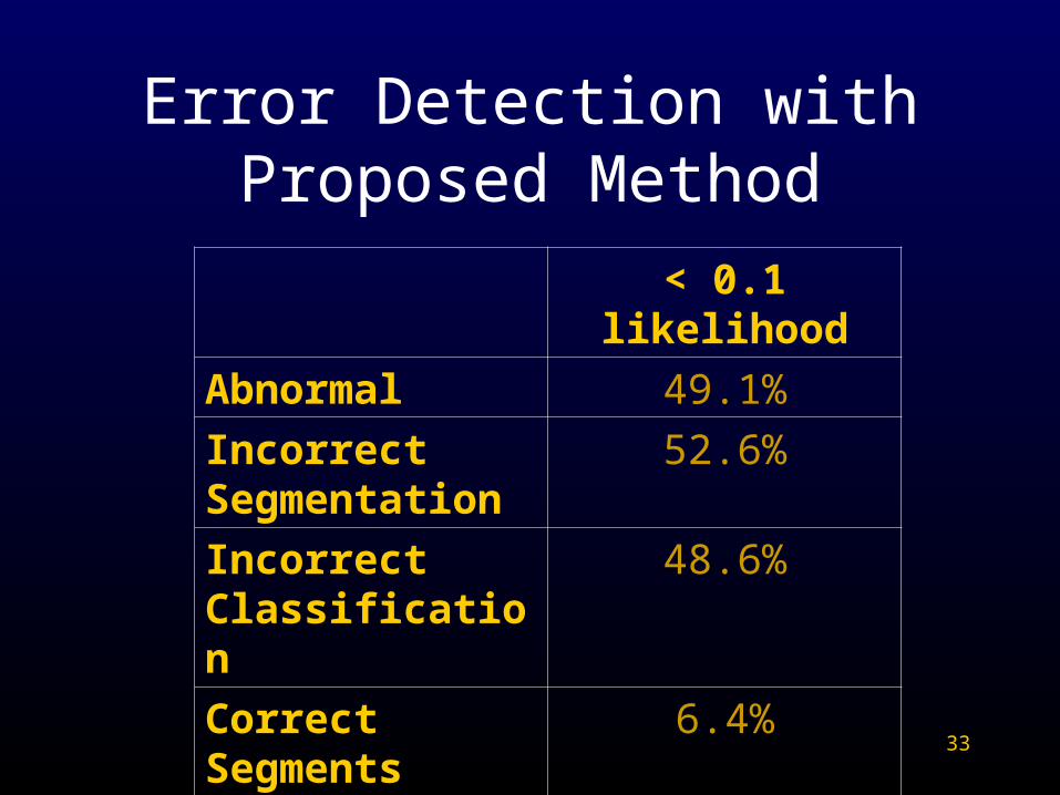
Error Detection withProposed Method

< 0.1 likelihood

Abnormal 49.1%

Incorrect Segmentation

52.6%

Incorrect Classification

48.6%

Correct Segments 6.4%

34

Contributions

• Derived single, unified maximum likelihood hypothesis test framework

• Decomposed chromosome clusters using M-FISH multi-spectral data

• Combined segmentation and classification for increased accuracy in both

• Demonstrated effective aberration scoring• Implemented joint segmentation-classification

algorithm in C (2-3 minutes/image on 167MHz Unix machine)

35

Future Work

• Improvements in likelihood function– Shape

– Number

• Pixel classification• Overcome “greedy” algorithm difficulties• Combine geometric, grayscale, and multi-spectral

information for complete algorithm