2 Huffman Coding

2Huffman Coding

Huffman coding is a popular method for compressing data with variable-length codes.Given a set of data symbols (an alphabet) and their frequencies of occurrence (or, equiv-alently, their probabilities), the method constructs a set of variable-length codewordswith the shortest average length and assigns them to the symbols. Huffman codingserves as the basis for several applications implemented on popular platforms. Someprograms use just the Huffman method, while others use it as one step in a multistepcompression process. The Huffman method [Huffman 52] is somewhat similar to theShannon–Fano method, proposed independently by Claude Shannon and Robert Fanoin the late 1940s ([Shannon 48] and [Fano 49]). It generally produces better codes, andlike the Shannon–Fano method, it produces the best variable-length codes when theprobabilities of the symbols are negative powers of 2. The main difference between thetwo methods is that Shannon–Fano constructs its codes from top to bottom (and thebits of each codeword are constructed from left to right), while Huffman constructs acode tree from the bottom up (and the bits of each codeword are constructed from rightto left).

Since its inception in 1952 by D. Huffman, the method has been the subject ofintensive research in data compression. The long discussion in [Gilbert and Moore 59]proves that the Huffman code is a minimum-length code in the sense that no otherencoding has a shorter average length. A much shorter proof of the same fact wasdiscovered by Huffman himself [Motil 07]. An algebraic approach to constructing theHuffman code is introduced in [Karp 61]. In [Gallager 78], Robert Gallager shows thatthe redundancy of Huffman coding is at most p1 + 0.086 where p1 is the probability ofthe most-common symbol in the alphabet. The redundancy is the difference betweenthe average Huffman codeword length and the entropy. Given a large alphabet, such

62 2. Huffman Coding

as the set of letters, digits and punctuation marks used by a natural language, thelargest symbol probability is typically around 15–20%, bringing the value of the quantityp1 + 0.086 to around 0.1. This means that Huffman codes are at most 0.1 bit longer(per symbol) than an ideal entropy encoder, such as arithmetic coding (Chapter 4).

This chapter describes the details of Huffman encoding and decoding and coversrelated topics such as the height of a Huffman code tree, canonical Huffman codes, andan adaptive Huffman algorithm. Following this, Section 2.4 illustrates an importantapplication of the Huffman method to facsimile compression.

David Huffman (1925–1999)

Being originally from Ohio, it is no wonder that Huffman went to Ohio State Uni-versity for his BS (in electrical engineering). What is unusual washis age (18) when he earned it in 1944. After serving in the UnitedStates Navy, he went back to Ohio State for an MS degree (1949)and then to MIT, for a PhD (1953, electrical engineering).

That same year, Huffman joined the faculty at MIT. In 1967,he made his only career move when he went to the University ofCalifornia, Santa Cruz as the founding faculty member of the Com-puter Science Department. During his long tenure at UCSC, Huff-man played a major role in the development of the department (heserved as chair from 1970 to 1973) and he is known for his motto“my products are my students.” Even after his retirement, in 1994, he remained activein the department, teaching information theory and signal analysis courses.

Huffman developed his celebrated algorithm as a term paper that he wrote in lieuof taking a final examination in an information theory class he took at MIT in 1951.The professor, Robert Fano, proposed the problem of constructing the shortest variable-length code for a set of symbols with known probabilities of occurrence.

It should be noted that in the late 1940s, Fano himself (and independently, alsoClaude Shannon) had developed a similar, but suboptimal, algorithm known today asthe Shannon–Fano method ([Shannon 48] and [Fano 49]). The difference between thetwo algorithms is that the Shannon–Fano code tree is built from the top down, whilethe Huffman code tree is constructed from the bottom up.

Huffman made significant contributions in several areas, mostly information theoryand coding, signal designs for radar and communications, and design procedures forasynchronous logical circuits. Of special interest is the well-known Huffman algorithmfor constructing a set of optimal prefix codes for data with known frequencies of occur-rence. At a certain point he became interested in the mathematical properties of “zerocurvature” surfaces, and developed this interest into techniques for folding paper intounusual sculptured shapes (the so-called computational origami).

2.1 Huffman Encoding 63

2.1 Huffman Encoding

The Huffman encoding algorithm starts by constructing a list of all the alphabet symbolsin descending order of their probabilities. It then constructs, from the bottom up, abinary tree with a symbol at every leaf. This is done in steps, where at each step twosymbols with the smallest probabilities are selected, added to the top of the partial tree,deleted from the list, and replaced with an auxiliary symbol representing the two originalsymbols. When the list is reduced to just one auxiliary symbol (representing the entirealphabet), the tree is complete. The tree is then traversed to determine the codewordsof the symbols.

This process is best illustrated by an example. Given five symbols with probabilitiesas shown in Figure 2.1a, they are paired in the following order:1. a4 is combined with a5 and both are replaced by the combined symbol a45, whoseprobability is 0.2.2. There are now four symbols left, a1, with probability 0.4, and a2, a3, and a45, withprobabilities 0.2 each. We arbitrarily select a3 and a45 as the two symbols with smallestprobabilities, combine them, and replace them with the auxiliary symbol a345, whoseprobability is 0.4.3. Three symbols are now left, a1, a2, and a345, with probabilities 0.4, 0.2, and 0.4,respectively. We arbitrarily select a2 and a345, combine them, and replace them withthe auxiliary symbol a2345, whose probability is 0.6.4. Finally, we combine the two remaining symbols, a1 and a2345, and replace them witha12345 with probability 1.

The tree is now complete. It is shown in Figure 2.1a “lying on its side” with itsroot on the right and its five leaves on the left. To assign the codewords, we arbitrarilyassign a bit of 1 to the top edge, and a bit of 0 to the bottom edge, of every pair ofedges. This results in the codewords 0, 10, 111, 1101, and 1100. The assignments of bitsto the edges is arbitrary.

The average size of this code is 0.4× 1 + 0.2× 2 + 0.2× 3 + 0.1× 4 + 0.1× 4 = 2.2bits/symbol, but even more importantly, the Huffman code is not unique. Some of thesteps above were chosen arbitrarily, because there were more than two symbols withsmallest probabilities. Figure 2.1b shows how the same five symbols can be combineddifferently to obtain a different Huffman code (11, 01, 00, 101, and 100). The averagesize of this code is 0.4 × 2 + 0.2 × 2 + 0.2 × 2 + 0.1 × 3 + 0.1 × 3 = 2.2 bits/symbol, thesame as the previous code.

� Exercise 2.1: Given the eight symbols A, B, C, D, E, F, G, and H with probabilities1/30, 1/30, 1/30, 2/30, 3/30, 5/30, 5/30, and 12/30, draw three different Huffman treeswith heights 5 and 6 for these symbols and compute the average code size for each tree.

� Exercise 2.2: Figure Ans.1d shows another Huffman tree, with height 4, for the eightsymbols introduced in Exercise 2.1. Explain why this tree is wrong.

It turns out that the arbitrary decisions made in constructing the Huffman treeaffect the individual codes but not the average size of the code. Still, we have to answerthe obvious question, which of the different Huffman codes for a given set of symbolsis best? The answer, while not obvious, is simple: The best code is the one with the


0.4

0.1

0.2

0.2

0.1

0.4

0.1

0.2

0.2

0.1

(a) (b)

a3

a345

a4

a45

a5

a2

a2345

a12345a1

a3

a4

a5

a2

a23

a45

a1 a145

0.2

0.4

0

0

0

0

0

0

0

0

1

1

1

1

0.2

0.4

0.6

1

1

11

1.00.6

1.0

Figure 2.1: Huffman Codes.

smallest variance. The variance of a code measures how much the sizes of the individualcodewords deviate from the average size. The variance of the code of Figure 2.1a is

0.4(1 − 2.2)2 + 0.2(2 − 2.2)2 + 0.2(3 − 2.2)2 + 0.1(4 − 2.2)2 + 0.1(4 − 2.2)2 = 1.36,

while the variance of code 2.1b is

0.4(2 − 2.2)2 + 0.2(2 − 2.2)2 + 0.2(2 − 2.2)2 + 0.1(3 − 2.2)2 + 0.1(3 − 2.2)2 = 0.16.

Code 2.1b is therefore preferable (see below). A careful look at the two trees shows howto select the one we want. In the tree of Figure 2.1a, symbol a45 is combined with a3,whereas in the tree of 2.1b a45 is combined with a1. The rule is: When there are morethan two smallest-probability nodes, select the ones that are lowest and highest in thetree and combine them. This will combine symbols of low probability with symbols ofhigh probability, thereby reducing the total variance of the code.

If the encoder simply writes the compressed data on a file, the variance of the codemakes no difference. A small-variance Huffman code is preferable only in cases wherethe encoder transmits the compressed data, as it is being generated, over a network. Insuch a case, a code with large variance causes the encoder to generate bits at a rate thatvaries all the time. Since the bits have to be transmitted at a constant rate, the encoderhas to use a buffer. Bits of the compressed data are entered into the buffer as they arebeing generated and are moved out of it at a constant rate, to be transmitted. It is easyto see intuitively that a Huffman code with zero variance will enter bits into the bufferat a constant rate, so only a short buffer will be needed. The larger the code variance,the more variable is the rate at which bits enter the buffer, requiring the encoder to usea larger buffer.

The following claim is sometimes found in the literature:It can be shown that the size of the Huffman code of a symbolai with probability Pi is always less than or equal to �− log2 Pi�.

2.1 Huffman Encoding 65

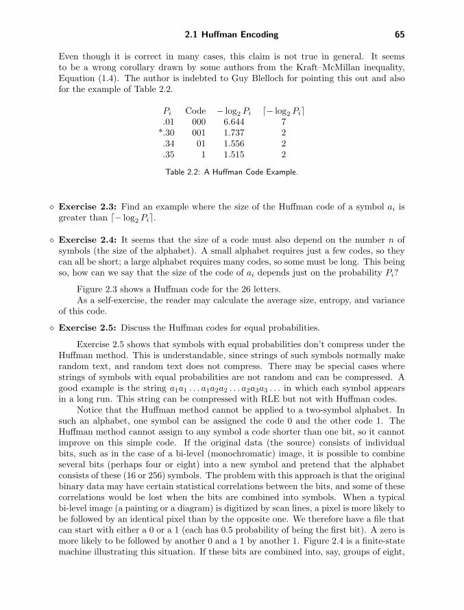
Even though it is correct in many cases, this claim is not true in general. It seemsto be a wrong corollary drawn by some authors from the Kraft–McMillan inequality,Equation (1.4). The author is indebted to Guy Blelloch for pointing this out and alsofor the example of Table 2.2.

Pi Code − log2 Pi �− log2 Pi�.01 000 6.644 7

*.30 001 1.737 2.34 01 1.556 2.35 1 1.515 2

Table 2.2: A Huffman Code Example.

� Exercise 2.3: Find an example where the size of the Huffman code of a symbol ai isgreater than �− log2 Pi�.

� Exercise 2.4: It seems that the size of a code must also depend on the number n ofsymbols (the size of the alphabet). A small alphabet requires just a few codes, so theycan all be short; a large alphabet requires many codes, so some must be long. This beingso, how can we say that the size of the code of ai depends just on the probability Pi?

Figure 2.3 shows a Huffman code for the 26 letters.As a self-exercise, the reader may calculate the average size, entropy, and variance

of this code.

� Exercise 2.5: Discuss the Huffman codes for equal probabilities.

Exercise 2.5 shows that symbols with equal probabilities don’t compress under theHuffman method. This is understandable, since strings of such symbols normally makerandom text, and random text does not compress. There may be special cases wherestrings of symbols with equal probabilities are not random and can be compressed. Agood example is the string a1a1 . . . a1a2a2 . . . a2a3a3 . . . in which each symbol appearsin a long run. This string can be compressed with RLE but not with Huffman codes.

Notice that the Huffman method cannot be applied to a two-symbol alphabet. Insuch an alphabet, one symbol can be assigned the code 0 and the other code 1. TheHuffman method cannot assign to any symbol a code shorter than one bit, so it cannotimprove on this simple code. If the original data (the source) consists of individualbits, such as in the case of a bi-level (monochromatic) image, it is possible to combineseveral bits (perhaps four or eight) into a new symbol and pretend that the alphabetconsists of these (16 or 256) symbols. The problem with this approach is that the originalbinary data may have certain statistical correlations between the bits, and some of thesecorrelations would be lost when the bits are combined into symbols. When a typicalbi-level image (a painting or a diagram) is digitized by scan lines, a pixel is more likely tobe followed by an identical pixel than by the opposite one. We therefore have a file thatcan start with either a 0 or a 1 (each has 0.5 probability of being the first bit). A zero ismore likely to be followed by another 0 and a 1 by another 1. Figure 2.4 is a finite-statemachine illustrating this situation. If these bits are combined into, say, groups of eight,


000 E .1300 0010 T .0900 0011 A .0800 0100 O .0800

0101 N .07000110 R .06500111 I .0650

10000 H .060010001 S .060010010 D .040010011 L .035010100 C .030010101 U .030010110 M .030010111 F .020011000 P .020011001 Y .020011010 B .015011011 W .015011100 G .015011101 V .0100111100 J .0050111101 K .0050111110 X .0050

1111110 Q .00251111111 Z .0025 .005

.11

.010

.010.020

.025

.045

.070

.115

.305

.420

.580

.30

.28

.1951.0

1

1

00

1

0

10

01

0

1

Figure 2.3: A Huffman Code for the 26-Letter Alphabet.

the bits inside a group will still be correlated, but the groups themselves will not becorrelated by the original pixel probabilities. If the input data contains, e.g., the twoadjacent groups 00011100 and 00001110, they will be encoded independently, ignoringthe correlation between the last 0 of the first group and the first 0 of the next group.Selecting larger groups improves this situation but increases the number of groups, whichimplies more storage for the code table and longer time to calculate the table.

� Exercise 2.6: How does the number of groups increase when the group size increasesfrom s bits to s + n bits?

A more complex approach to image compression by Huffman coding is to createseveral complete sets of Huffman codes. If the group size is, e.g., eight bits, then severalsets of 256 codes are generated. When a symbol S is to be encoded, one of the sets isselected, and S is encoded using its code in that set. The choice of set depends on thesymbol preceding S.

2.2 Huffman Decoding 67

0 1

s

0,50% 1,50%

0,40% 1,60%

1,33%

0,67%

Start

Figure 2.4: A Finite-State Machine.

� Exercise 2.7: Imagine an image with 8-bit pixels where half the pixels have values 127and the other half have values 128. Analyze the performance of RLE on the individualbitplanes of such an image, and compare it with what can be achieved with Huffmancoding.

Which two integers come next in the infinite sequence 38, 24, 62, 12, 74, . . . ?

2.2 Huffman Decoding

Before starting the compression of a data file, the compressor (encoder) has to determinethe codes. It does that based on the probabilities (or frequencies of occurrence) of thesymbols. The probabilities or frequencies have to be written, as side information, onthe output, so that any Huffman decompressor (decoder) will be able to decompressthe data. This is easy, because the frequencies are integers and the probabilities canbe written as scaled integers. It normally adds just a few hundred bytes to the output.It is also possible to write the variable-length codes themselves on the output, but thismay be awkward, because the codes have different sizes. It is also possible to write theHuffman tree on the output, but this may require more space than just the frequencies.

In any case, the decoder must know what is at the start of the compressed file,read it, and construct the Huffman tree for the alphabet. Only then can it read anddecode the rest of its input. The algorithm for decoding is simple. Start at the rootand read the first bit off the input (the compressed file). If it is zero, follow the bottomedge of the tree; if it is one, follow the top edge. Read the next bit and move anotheredge toward the leaves of the tree. When the decoder arrives at a leaf, it finds there theoriginal, uncompressed symbol (normally its ASCII code), and that code is emitted bythe decoder. The process starts again at the root with the next bit.

This process is illustrated for the five-symbol alphabet of Figure 2.5. The four-symbol input string a4a2a5a1 is encoded into 1001100111. The decoder starts at theroot, reads the first bit 1, and goes up. The second bit 0 sends it down, as does thethird bit. This brings the decoder to leaf a4, which it emits. It again returns to theroot, reads 110, moves up, up, and down, to reach leaf a2, and so on.


1

2

3

4

5

1

1

0

0

Figure 2.5: Huffman Codes for Equal Probabilities.

2.2.1 Fast Huffman Decoding

Decoding a Huffman-compressed file by sliding down the code tree for each symbol isconceptually simple, but slow. The compressed file has to be read bit by bit and thedecoder has to advance a node in the code tree for each bit. The method of this section,originally conceived by [Choueka et al. 85] but later reinvented by others, uses presetpartial-decoding tables. These tables depend on the particular Huffman code used, butnot on the data to be decoded. The compressed file is read in chunks of k bits each(where k is normally 8 or 16 but can have other values) and the current chunk is usedas a pointer to a table. The table entry that is selected in this way can decode severalsymbols and it also points the decoder to the table to be used for the next chunk.

As an example, consider the Huffman code of Figure 2.1a, where the five codewordsare 0, 10, 111, 1101, and 1100. The string of symbols a1a1a2a4a3a1a5 . . . is compressedby this code to the string 0|0|10|1101|111|0|1100 . . .. We select k = 3 and read this stringin 3-bit chunks 001|011|011|110|110|0 . . .. Examining the first chunk, it is easy to seethat it should be decoded into a1a1 followed by the single bit 1 which is the prefix ofanother codeword. The first chunk is 001 = 110, so we set entry 1 of the first table (table0) to the pair (a1a1, 1). When chunk 001 is used as a pointer to table 0, it points to entry1, which immediately provides the decoder with the two decoded symbols a1a1 and alsodirects it to use table 1 for the next chunk. Table 1 is used when a partially-decodedchunk ends with the single-bit prefix 1. The next chunk is 011 = 310, so entry 3 oftable 1 corresponds to the encoded bits 1|011. Again, it is easy to see that these shouldbe decoded to a2 and there is the prefix 11 left over. Thus, entry 3 of table 1 should be(a2, 2). It provides the decoder with the single symbol a2 and also directs it to use table 2next (the table that corresponds to prefix 11). The next chunk is again 011 = 310, soentry 3 of table 2 corresponds to the encoded bits 11|011. It is again obvious that theseshould be decoded to a4 with a prefix of 1 left over. This process continues until theend of the encoded input. Figure 2.6 is the simple decoding algorithm in pseudocode.

Table 2.7 lists the four tables required to decode this code. It is easy to see thatthey correspond to the prefixes Λ (null), 1, 11, and 110. A quick glance at Figure 2.1ashows that these correspond to the root and the four interior nodes of the Huffman codetree. Thus, each partial-decoding table corresponds to one of the four prefixes of thiscode. The number m of partial-decoding tables therefore equals the number of interiornodes (plus the root) which is one less than the number N of symbols of the alphabet.


i←0; output←null;repeatj←input next chunk;(s,i)←Tablei[j];append s to output;

until end-of-input

Figure 2.6: Fast Huffman Decoding.

T0 = Λ T1 = 1 T2 = 11 T3 = 110000 a1a1a1 0 1|000 a2a1a1 0 11|000 a5a1 0 110|000 a5a1a1 0001 a1a1 1 1|001 a2a1 1 11|001 a5 1 110|001 a5a1 1010 a1a2 0 1|010 a2a2 0 11|010 a4a1 0 110|010 a5a2 0011 a1 2 1|011 a2 2 11|011 a4 1 110|011 a5 2100 a2a1 0 1|100 a5 0 11|100 a3a1a1 0 110|100 a4a1a1 0101 a2 1 1|101 a4 0 11|101 a3a1 1 110|101 a4a1 1110 − 3 1|110 a3a1 0 11|110 a3a2 0 110|110 a4a2 0111 a3 0 1|111 a3 1 11|111 a3 2 110|111 a4 2

Table 2.7: Partial-Decoding Tables for a Huffman Code.

Notice that some chunks (such as entry 110 of table 0) simply send the decoderto another table and do not provide any decoded symbols. Also, there is a trade-offbetween chunk size (and thus table size) and decoding speed. Large chunks speed updecoding, but require large tables. A large alphabet (such as the 128 ASCII charactersor the 256 8-bit bytes) also requires a large set of tables. The problem with large tablesis that the decoder has to set up the tables after it has read the Huffman codes from thecompressed stream and before decoding can start, and this process may preempt anygains in decoding speed provided by the tables.

To set up the first table (table 0, which corresponds to the null prefix Λ), thedecoder generates the 2k bit patterns 0 through 2k − 1 (the first column of Table 2.7)and employs the decoding method of Section 2.2 to decode each pattern. This yieldsthe second column of Table 2.7. Any remainders left are prefixes and are convertedby the decoder to table numbers. They become the third column of the table. If noremainder is left, the third column is set to 0 (use table 0 for the next chunk). Each ofthe other partial-decoding tables is set in a similar way. Once the decoder decides thattable 1 corresponds to prefix p, it generates the 2k patterns p|00 . . . 0 through p|11 . . . 1that become the first column of that table. It then decodes that column to generate theremaining two columns.

This method was conceived in 1985, when storage costs were considerably higherthan today (early 2007). This prompted the developers of the method to find ways tocut down the number of partial-decoding tables, but these techniques are less importanttoday and are not described here.


2.2.2 Average Code Size

Figure 2.8a shows a set of five symbols with their probabilities and a typical Huffmantree. Symbol A appears 55% of the time and is assigned a 1-bit code, so it contributes0.55 ·1 bits to the average code size. Symbol E appears only 2% of the time and isassigned a 4-bit Huffman code, so it contributes 0.02 ·4 = 0.08 bits to the code size. Theaverage code size is therefore easily computed as

0.55 · 1 + 0.25 · 2 + 0.15 · 3 + 0.03 · 4 + 0.02 · 4 = 1.7 bits per symbol.

Surprisingly, the same result is obtained by adding the values of the four internal nodesof the Huffman code tree 0.05 + 0.2 + 0.45 + 1 = 1.7. This provides a way to calculatethe average code size of a set of Huffman codes without any multiplications. Simply addthe values of all the internal nodes of the tree. Table 2.9 illustrates why this works.

A 0.55

B 0.25

C 0.15

D 0.03

E 0.02

0.05

0.2

0.45

1

0.02

0.03

0.051

d

(b)

(a)

ad−2

a1

Figure 2.8: Huffman Code Trees.

(Internal nodes are shown in italics in this table.) The left column consists of the valuesof all the internal nodes. The right columns show how each internal node is the sum of


.05 = .02+ .03

.20 = .05+ .15 = .02+ .03+ .15

.45 = .20+ .25 = .02+ .03+ .15+ .251 .0 = .45+ .55 = .02+ .03+ .15+ .25+ .55

Table 2.9: Composition of Nodes.

0 .05 = = 0.02 + 0.03 + · · ·a1 = 0 .05 + . . .= 0.02 + 0.03 + · · ·a2 = a1 + . . .= 0.02 + 0.03 + · · ·... =ad−2 = ad−3 + . . .= 0.02 + 0.03 + · · ·1 .0 = ad−2 + . . .= 0.02 + 0.03 + · · ·Table 2.10: Composition of Nodes.

some of the leaf nodes. Summing the values in the left column yields 1.7, and summingthe other columns shows that this 1.7 is the sum of the four values 0.02, the four values0.03, the three values 0.15, the two values 0.25, and the single value 0.55.

This argument can be extended to the general case. It is easy to show that, in aHuffman-like tree (a tree where each node is the sum of its children), the weighted sumof the leaves, where the weights are the distances of the leaves from the root, equalsthe sum of the internal nodes. (This property has been communicated to the author byJ. Motil.)

Figure 2.8b shows such a tree, where we assume that the two leaves 0.02 and 0.03have d-bit Huffman codes. Inside the tree, these leaves become the children of internalnode 0.05, which, in turn, is connected to the root by means of the d− 2 internal nodesa1 through ad−2. Table 2.10 has d rows and shows that the two values 0.02 and 0.03are included in the various internal nodes exactly d times. Adding the values of all theinternal nodes produces a sum that includes the contributions 0.02 · d + 0.03 · d fromthe two leaves. Since these leaves are arbitrary, it is clear that this sum includes similarcontributions from all the other leaves, so this sum is the average code size. Since thissum also equals the sum of the left column, which is the sum of the internal nodes, it isclear that the sum of the internal nodes equals the average code size.

Notice that this proof does not assume that the tree is binary. The property illus-trated here exists for any tree where a node contains the sum of its children.

2.2.3 Number of Codes

Since the Huffman code is not unique, the natural question is: How many different codesare there? Figure 2.11a shows a Huffman code tree for six symbols, from which we cananswer this question in two different ways as follows:

Answer 1. The tree of 2.11a has five interior nodes, and in general, a Huffman codetree for n symbols has n − 1 interior nodes. Each interior node has two edges comingout of it, labeled 0 and 1. Swapping the two labels produces a different Huffman codetree, so the total number of different Huffman code trees is 2n−1 (in our example, 25 or32). The tree of Figure 2.11b, for example, shows the result of swapping the labels ofthe two edges of the root. Table 2.12a,b lists the codes generated by the two trees.

Answer 2. The six codes of Table 2.12a can be divided into the four classes 00x,10y, 01, and 11, where x and y are 1-bit each. It is possible to create different Huffmancodes by changing the first two bits of each class. Since there are four classes, this isthe same as creating all the permutations of four objects, something that can be donein 4! = 24 ways. In each of the 24 permutations it is also possible to change the values


1

2

3

4

5

6

.11

.12

.13

.14

.24

.26

.11

.12

.13

.14

.24

.26

0

1

0

00

0

11

1

11

2

3

4

5

6

0

1

0

00

01

1

1

1

(a) (b)

000 100 000001 101 001100 000 010101 001 01101 11 1011 01 11

(a) (b) (c)

Figure 2.11: Two Huffman Code Trees. Table 2.12.

of x and y in four different ways (since they are bits) so the total number of differentHuffman codes in our six-symbol example is 24 × 4 = 96.

The two answers are different because they count different things. Answer 1 countsthe number of different Huffman code trees, while answer 2 counts the number of differentHuffman codes. It turns out that our example can generate 32 different code trees butonly 94 different codes instead of 96. This shows that there are Huffman codes thatcannot be generated by the Huffman method! Table 2.12c shows such an example. Alook at the trees of Figure 2.11 should convince the reader that the codes of symbols 5and 6 must start with different bits, but in the code of Table 2.12c they both start with1. This code is therefore impossible to generate by any relabeling of the nodes of thetrees of Figure 2.11.

2.2.4 Ternary Huffman Codes

The Huffman code is not unique. Moreover, it does not have to be binary! The Huffmanmethod can easily be applied to codes based on other number systems. Figure 2.13ashows a Huffman code tree for five symbols with probabilities 0.15, 0.15, 0.2, 0.25, and0.25. The average code size is

2×0.25 + 3×0.15 + 3×0.15 + 2×0.20 + 2×0.25 = 2.3 bits/symbol.

Figure 2.13b shows a ternary Huffman code tree for the same five symbols. The treeis constructed by selecting, at each step, three symbols with the smallest probabilitiesand merging them into one parent symbol, with the combined probability. The averagecode size of this tree is

2×0.15 + 2×0.15 + 2×0.20 + 1×0.25 + 1×0.25 = 1.5 trits/symbol.

Notice that the ternary codes use the digits 0, 1, and 2.

� Exercise 2.8: Given seven symbols with probabilities 0.02, 0.03, 0.04, 0.04, 0.12, 0.26,and 0.49, construct binary and ternary Huffman code trees for them and calculate theaverage code size in each case.


(a)

.15 .15 .20 .15 .15 .20

.50 .25 .25

.25

.45.30.25

.55

1.0

1.0

(b)

(c) (d)

.02 .03 .04 .02 .03 .04

.09 .04 .12

.26 .25 .49

.04

.08

.13 .12

.25.26

.51.49

1.0

1.0

.05

Figure 2.13: Binary and Ternary Huffman Code Trees.

2.2.5 Height of a Huffman Tree

The height of the code tree generated by the Huffman algorithm may sometimes beimportant because the height is also the length of the longest code in the tree. TheDeflate method (Section 3.3), for example, limits the lengths of certain Huffman codesto just three bits.

It is easy to see that the shortest Huffman tree is created when the symbols haveequal probabilities. If the symbols are denoted by A, B, C, and so on, then the algorithmcombines pairs of symbols, such A and B, C and D, in the lowest level, and the rest of thetree consists of interior nodes as shown in Figure 2.14a. The tree is balanced or closeto balanced and its height is �log2 n�. In the special case where the number of symbolsn is a power of 2, the height is exactly log2 n. In order to generate the tallest tree, we


need to assign probabilities to the symbols such that each step in the Huffman methodwill increase the height of the tree by 1. Recall that each step in the Huffman algorithmcombines two symbols. Thus, the tallest tree is obtained when the first step combinestwo of the n symbols and each subsequent step combines the result of its predecessorwith one of the remaining symbols (Figure 2.14b). The height of the complete tree istherefore n − 1, and it is referred to as a lopsided or unbalanced tree.

It is easy to see what symbol probabilities result in such a tree. Denote the twosmallest probabilities by a and b. They are combined in the first step to form a nodewhose probability is a + b. The second step will combine this node with an originalsymbol if one of the symbols has probability a + b (or smaller) and all the remainingsymbols have greater probabilities. Thus, after the second step, the root of the treehas probability a + b + (a + b) and the third step will combine this root with one ofthe remaining symbols if its probability is a + b + (a + b) and the probabilities of theremaining n− 4 symbols are greater. It does not take much to realize that the symbolshave to have probabilities p1 = a, p2 = b, p3 = a+b = p1 +p2, p4 = b+(a+b) = p2 +p3,p5 = (a + b) + (a + 2b) = p3 + p4, p6 = (a + 2b) + (2a + 3b) = p4 + p5, and so on(Figure 2.14c). These probabilities form a Fibonacci sequence whose first two elementsare a and b. As an example, we select a = 5 and b = 2 and generate the 5-numberFibonacci sequence 5, 2, 7, 9, and 16. These five numbers add up to 39, so dividingthem by 39 produces the five probabilities 5/39, 2/39, 7/39, 9/39, and 15/39. TheHuffman tree generated by them has a maximal height (which is 4).

000 001 010 011 100 101 110 111

(a) (b) (c)

a+b

a+2b

2a+3b

3a+5b

5a+8b

a b

0

10

110

1110

11110 11111

Figure 2.14: Shortest and Tallest Huffman Trees.

In principle, symbols in a set can have any probabilities, but in practice, the proba-bilities of symbols in an input file are computed by counting the number of occurrencesof each symbol. Imagine a text file where only the nine symbols A through I appear.In order for such a file to produce the tallest Huffman tree, where the codes will havelengths from 1 to 8 bits, the frequencies of occurrence of the nine symbols have to form aFibonacci sequence of probabilities. This happens when the frequencies of the symbolsare 1, 1, 2, 3, 5, 8, 13, 21, and 34 (or integer multiples of these). The sum of thesefrequencies is 88, so our file has to be at least that long in order for a symbol to have8-bit Huffman codes. Similarly, if we want to limit the sizes of the Huffman codes of aset of n symbols to 16 bits, we need to count frequencies of at least 4,180 symbols. Tolimit the code sizes to 32 bits, the minimum data size is 9,227,464 symbols.


If a set of symbols happens to have the Fibonacci probabilities and therefore resultsin a maximal-height Huffman tree with codes that are too long, the tree can be reshaped(and the maximum code length shortened) by slightly modifying the symbol probabil-ities, so they are not much different from the original, but do not form a Fibonaccisequence.

2.2.6 Canonical Huffman Codes

The code of Table 2.12c has a simple interpretation. It assigns the first four symbols the3-bit codes 0, 1, 2, and 3, and the last two symbols the 2-bit codes 2 and 3. This is anexample of a canonical Huffman code. The word “canonical” means that this particularcode has been selected from among the several (or even many) possible Huffman codesbecause its properties make it easy and fast to use.

Canonical (adjective): Conforming to orthodox or well-established rules or patterns,as of procedure.

Table 2.15 shows a slightly bigger example of a canonical Huffman code. Imaginea set of 16 symbols (whose probabilities are irrelevant and are not shown) such thatfour symbols are assigned 3-bit codes, five symbols are assigned 5-bit codes, and theremaining seven symbols are assigned 6-bit codes. Table 2.15a shows a set of possibleHuffman codes, while Table 2.15b shows a set of canonical Huffman codes. It is easy tosee that the seven 6-bit canonical codes are simply the 6-bit integers 0 through 6. Thefive codes are the 5-bit integers 4 through 8, and the four codes are the 3-bit integers 3through 6. We first show how these codes are generated and then how they are used.

1: 000 011 9: 10100 010002: 001 100 10: 101010 0000003: 010 101 11: 101011 0000014: 011 110 12: 101100 0000105: 10000 00100 13: 101101 0000116: 10001 00101 14: 101110 0001007: 10010 00110 15: 101111 0001018: 10011 00111 16: 110000 000110

(a) (b) (a) (b)

length: 1 2 3 4 5 6numl: 0 0 4 0 5 7first: 2 4 3 5 4 0

Table 2.15. Table 2.16.

The top row (length) of Table 2.16 lists the possible code lengths, from 1 to 6 bits.The second row (numl) lists the number of codes of each length, and the bottom row(first) lists the first code in each group. This is why the three groups of codes start withvalues 3, 4, and 0. To obtain the top two rows we need to compute the lengths of allthe Huffman codes for the given alphabet (see below). The third row is computed bysetting “first[6]:=0;” and iterating

for l:=5 downto 1 do first[l]:=�(first[l+1]+numl[l+1])/2�;This guarantees that all the 3-bit prefixes of codes longer than three bits will be lessthan first[3] (which is 3), all the 5-bit prefixes of codes longer than five bits will beless than first[5] (which is 4), and so on.


Now for the use of these unusual codes. Canonical Huffman codes are useful incases where the alphabet is large and where fast decoding is mandatory. Because of theway the codes are constructed, it is easy for the decoder to identify the length of a codeby reading and examining input bits one by one. Once the length is known, the symbolcan be found in one step. The pseudocode listed here shows the rules for decoding:

l:=1; input v;while v<first[l]append next input bit to v; l:=l+1;endwhile

As an example, suppose that the next code is 00110. As bits are input and appendedto v, it goes through the values 0, 00 = 0, 001 = 1, 0011 = 3, 00110 = 6, while l isincremented from 1 to 5. All steps except the last satisfy v<first[l], so the laststep determines the value of l (the code length) as 5. The symbol itself is found bysubtracting v− first[5] = 6− 4 = 2, so it is the third symbol (numbering starts at 0)in group l = 5 (symbol 7 of the 16 symbols).

The last point to be discussed is the encoder. In order to construct the canoni-cal Huffman code, the encoder needs to know the length of the Huffman code of everysymbol. The main problem is the large size of the alphabet, which may make it imprac-tical or even impossible to build the entire Huffman code tree in memory. There is analgorithm—described in [Hirschberg and Lelewer 90], [Sieminski 88], and [Salomon 07]—that solves this problem. It calculates the code sizes for an alphabet of n symbols usingjust one array of size 2n.

Considine’s Law. Whenever one word or letter can change the entire meaning of asentence, the probability of an error being made will be in direct proportion to theembarrassment it will cause.

—Bob Considine

One morning I was on my way to the market and met a man with four wives(perfectly legal where we come from). Each wife had four bags, containing four dogseach, and each dog had four puppies. The question is (think carefully) how many weregoing to the market?

2.3 Adaptive Huffman Coding

The Huffman method assumes that the frequencies of occurrence of all the symbols ofthe alphabet are known to the compressor. In practice, the frequencies are seldom, ifever, known in advance. One approach to this problem is for the compressor to read theoriginal data twice. The first time, it only counts the frequencies; the second time, itcompresses the data. Between the two passes, the compressor constructs the Huffmantree. Such a two-pass method is sometimes called semiadaptive and is normally too slowto be practical. The method that is used in practice is called adaptive (or dynamic)Huffman coding. This method is the basis of the UNIX compact program. The method

2.3 Adaptive Huffman Coding 77

was originally developed by [Faller 73] and [Gallager 78] with substantial improvementsby [Knuth 85].

The main idea is for the compressor and the decompressor to start with an emptyHuffman tree and to modify it as symbols are being read and processed (in the case of thecompressor, the word “processed” means compressed; in the case of the decompressor, itmeans decompressed). The compressor and decompressor should modify the tree in thesame way, so at any point in the process they should use the same codes, although thosecodes may change from step to step. We say that the compressor and decompressorare synchronized or that they work in lockstep (although they don’t necessarily worktogether; compression and decompression normally take place at different times). Theterm mirroring is perhaps a better choice. The decoder mirrors the operations of theencoder.

Initially, the compressor starts with an empty Huffman tree. No symbols have beenassigned codes yet. The first symbol being input is simply written on the output in itsuncompressed form. The symbol is then added to the tree and a code assigned to it.The next time this symbol is encountered, its current code is written on the output, andits frequency incremented by 1. Since this modifies the tree, it (the tree) is examined tosee whether it is still a Huffman tree (best codes). If not, it is rearranged, an operationthat results in modified codes.

The decompressor mirrors the same steps. When it reads the uncompressed formof a symbol, it adds it to the tree and assigns it a code. When it reads a compressed(variable-length) code, it scans the current tree to determine what symbol the codebelongs to, and it increments the symbol’s frequency and rearranges the tree in thesame way as the compressor.

It is immediately clear that the decompressor needs to know whether the itemit has just input is an uncompressed symbol (normally, an 8-bit ASCII code, but seeSection 2.3.1) or a variable-length code. To remove any ambiguity, each uncompressedsymbol is preceded by a special, variable-size escape code. When the decompressor readsthis code, it knows that the next eight bits are the ASCII code of a symbol that appearsin the compressed file for the first time.

Escape is not his plan. I must face him. Alone.—David Prowse as Lord Darth Vader in Star Wars (1977)

The trouble is that the escape code should not be any of the variable-length codesused for the symbols. These codes, however, are being modified every time the tree isrearranged, which is why the escape code should also be modified. A natural way to dothis is to add an empty leaf to the tree, a leaf with a zero frequency of occurrence, that’salways assigned to the 0-branch of the tree. Since the leaf is in the tree, it is assigneda variable-length code. This code is the escape code preceding every uncompressedsymbol. As the tree is being rearranged, the position of the empty leaf—and thus itscode—change, but this escape code is always used to identify uncompressed symbols inthe compressed file. Figure 2.17 shows how the escape code moves and changes as thetree grows.


1 0

0 1 0

1 0

0

1

1 0

1 0

1 0 1 0

1 0

0

000Figure 2.17: The Escape Code.

2.3.1 Uncompressed Codes

If the symbols being compressed are ASCII characters, they may simply be assignedtheir ASCII codes as uncompressed codes. In the general case where there may be anysymbols, uncompressed codes of two different sizes can be assigned by a simple method.Here is an example for the case n = 24. The first 16 symbols can be assigned the numbers0 through 15 as their codes. These numbers require only 4 bits, but we encode them in 5bits. Symbols 17 through 24 can be assigned the numbers 17−16−1 = 0, 18−16−1 = 1through 24−16−1 = 7 as 4-bit numbers. We end up with the sixteen 5-bit codes 00000,00001, . . . , 01111, followed by the eight 4-bit codes 0000, 0001, . . . , 0111.

In general, we assume an alphabet that consists of the n symbols a1, a2, . . . , an. Weselect integers m and r such that 2m ≤ n < 2m+1 and r = n− 2m. The first 2m symbolsare encoded as the (m + 1)-bit numbers 0 through 2m − 1. The remaining symbols areencoded as m-bit numbers such that the code of ak is k − 2m − 1. This code is alsocalled a phased-in binary code (also a minimal binary code).

2.3.2 Modifying the Tree

The chief principle for modifying the tree is to check it each time a symbol is input. Ifthe tree is no longer a Huffman tree, it should be rearranged to become one. A glanceat Figure 2.18a shows what it means for a binary tree to be a Huffman tree. The tree inthe figure contains five symbols: A, B, C, D, and E. It is shown with the symbols andtheir frequencies (in parentheses) after 16 symbols have been input and processed. Theproperty that makes it a Huffman tree is that if we scan it level by level, scanning eachlevel from left to right, and going from the bottom (the leaves) to the top (the root),the frequencies will be in sorted, nondescending order. Thus, the bottom-left node (A)has the lowest frequency, and the top-right node (the root) has the highest frequency.This is called the sibling property.

� Exercise 2.9: Why is this the criterion for a tree to be a Huffman tree?

Here is a summary of the operations needed to update the tree. The loop startsat the current node (the one corresponding to the symbol just input). This node is aleaf that we denote by X, with frequency of occurrence F . Each iteration of the loopinvolves three steps as follows:

1. Compare X to its successors in the tree (from left to right and bottom to top). Ifthe immediate successor has frequency F + 1 or greater, the nodes are still in sortedorder and there is no need to change anything. Otherwise, some successors of X have


identical frequencies of F or smaller. In this case, X should be swapped with the lastnode in this group (except that X should not be swapped with its parent).2. Increment the frequency of X from F to F + 1. Increment the frequencies of all itsparents.3. If X is the root, the loop stops; otherwise, it repeats with the parent of node X.

Figure 2.18b shows the tree after the frequency of node A has been incrementedfrom 1 to 2. It is easy to follow the three rules above to see how incrementing thefrequency of A results in incrementing the frequencies of all its parents. No swaps areneeded in this simple case because the frequency of A hasn’t exceeded the frequency ofits immediate successor B. Figure 2.18c shows what happens when A’s frequency hasbeen incremented again, from 2 to 3. The three nodes following A, namely, B, C, andD, have frequencies of 2, so A is swapped with the last of them, D. The frequenciesof the new parents of A are then incremented, and each is compared with its successor,but no more swaps are needed.

Figure 2.18d shows the tree after the frequency of A has been incremented to 4.Once we decide that A is the current node, its frequency (which is still 3) is compared tothat of its successor (4), and the decision is not to swap. A’s frequency is incremented,followed by incrementing the frequencies of its parents.

In Figure 2.18e, A is again the current node. Its frequency (4) equals that of itssuccessor, so they should be swapped. This is shown in Figure 2.18f, where A’s frequencyis 5. The next loop iteration examines the parent of A, with frequency 10. It shouldbe swapped with its successor E (with frequency 9), which leads to the final tree ofFigure 2.18g.

2.3.3 Counter Overflow

The frequency counts are accumulated in the Huffman tree in fixed-size fields, andsuch fields may overflow. A 16-bit unsigned field can accommodate counts of up to216 − 1 = 65,535. A simple solution to the counter overflow problem is to watch thecount field of the root each time it is incremented, and when it reaches its maximumvalue, to rescale all the frequency counts by dividing them by 2 (integer division). Inpractice, this is done by dividing the count fields of the leaves, then updating the countsof the interior nodes. Each interior node gets the sum of the counts of its children. Theproblem is that the counts are integers, and integer division reduces precision. This maychange a Huffman tree to one that does not satisfy the sibling property.

A simple example is shown in Figure 2.18h. After the counts of the leaves are halved,the three interior nodes are updated as shown in Figure 2.18i. The latter tree, however,is no longer a Huffman tree, since the counts are no longer in sorted order. The solutionis to rebuild the tree each time the counts are rescaled, which does not happen veryoften. A Huffman data compression program intended for general use should thereforehave large count fields that would not overflow very often. A 4-byte count field overflowsat 232 − 1 ≈ 4.3 × 109.

It should be noted that after rescaling the counts, the new symbols being read andcompressed have more effect on the counts than the old symbols (those counted beforethe rescaling). This turns out to be fortuitous since it is known from experience thatthe probability of appearance of a symbol depends more on the symbols immediatelypreceding it than on symbols that appeared in the distant past.


A B C D

E

(1) (2) (2) (2)

(3) (4)

(16)

(9)

(7)

AB CD

E

(2) (2) (2) (3)

(4) (9)

A B C D

E

(2) (2) (2)

(9)

AB CD

E

(2) (2) (2) (4)

(4) (6)(9)

(10)

AB CD

E

(2) (2) (2) (4)

(4) (6)

(19)

(9)(10)

A

B

C

D

E

(2) (2)

(2)

(5)(4)

(6)

(19)

(9)

(10)

A

B

C

D

E

(2) (2)

(2)

(5)(4)

(6)(9)

(11)

(20)

155 155 310 310

310 620

930

77 77 155 155

154 310

464

(a)

(19)

(2)

(4) (4)

(8)

(17) (18)

(9)

(5)

(b) (c)

(d) (e) (f)

(g) (h) (i)

Figure 2.18: Updating the Huffman Tree.


2.3.4 Code Overflow

An even more serious problem is code overflow. This may happen when many symbolsare added to the tree, and it becomes tall. The codes themselves are not stored in thetree, since they change all the time, and the compressor has to figure out the code of asymbol X each time X is input. Here are the details of this process:

1. The encoder has to locate symbol X in the tree. The tree has to be implemented asan array of structures, each a node, and the array is searched linearly.2. If X is not found, the escape code is emitted, followed by the uncompressed code ofX. X is then added to the tree.3. If X is found, the compressor moves from node X back to the root, building thecode bit by bit as it goes along. Each time it goes from a left child to a parent, a “1”is appended to the code. Going from a right child to a parent appends a “0” bit to thecode (or vice versa, but this should be consistent because it is mirrored by the decoder).Those bits have to be accumulated someplace, since they have to be emitted in thereverse order in which they are created. When the tree gets taller, the codes get longer.If they are accumulated in a 16-bit integer, then codes longer than 16 bits would causea malfunction.

One solution to the code overflow problem is to accumulate the bits of a code in alinked list, where new nodes can be created, limited in number only by the amount ofavailable memory. This is general but slow. Another solution is to accumulate the codesin a large integer variable (perhaps 50 bits wide) and document a maximum code sizeof 50 bits as one of the limitations of the program.

Fortunately, this problem does not affect the decoding process. The decoder readsthe compressed code bit by bit and uses each bit to move one step left or right downthe tree until it reaches a leaf node. If the leaf is the escape code, the decoder reads theuncompressed code of the symbol off the compressed data (and adds the symbol to thetree). Otherwise, the uncompressed code is found in the leaf node.

� Exercise 2.10: Given the 11-symbol string sir�sid�is, apply the adaptive Huffmanmethod to it. For each symbol input, show the output, the tree after the symbol hasbeen added to it, the tree after being rearranged (if necessary), and the list of nodestraversed left to right and bottom up.

2.3.5 A Variant

This variant of the adaptive Huffman method is simpler but less efficient. The ideais to calculate a set of n variable-length codes based on equal probabilities, to assignthose codes to the n symbols at random, and to change the assignments “on the fly,” assymbols are being read and compressed. The method is inefficient because the codes arenot based on the actual probabilities of the symbols in the input. However, it is simplerto implement and also faster than the adaptive method described earlier, because it hasto swap rows in a table, rather than update a tree, when updating the frequencies ofthe symbols.

The main data structure is an n× 3 table where the three columns store the namesof the n symbols, their frequencies of occurrence so far, and their codes. The table isalways kept sorted by the second column. When the frequency counts in the second


Name Count Codea1 0 0a2 0 10a3 0 110a4 0 111

(a)


(b)


(c)


(d)

Table 2.19: Four Steps in a Huffman Variant.

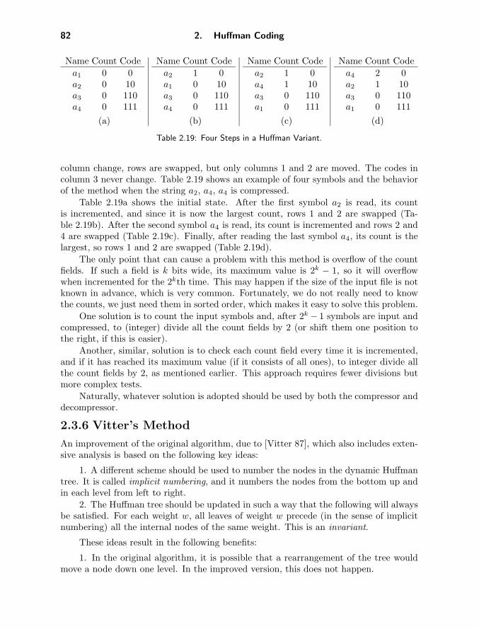
column change, rows are swapped, but only columns 1 and 2 are moved. The codes incolumn 3 never change. Table 2.19 shows an example of four symbols and the behaviorof the method when the string a2, a4, a4 is compressed.

Table 2.19a shows the initial state. After the first symbol a2 is read, its countis incremented, and since it is now the largest count, rows 1 and 2 are swapped (Ta-ble 2.19b). After the second symbol a4 is read, its count is incremented and rows 2 and4 are swapped (Table 2.19c). Finally, after reading the last symbol a4, its count is thelargest, so rows 1 and 2 are swapped (Table 2.19d).

The only point that can cause a problem with this method is overflow of the countfields. If such a field is k bits wide, its maximum value is 2k − 1, so it will overflowwhen incremented for the 2kth time. This may happen if the size of the input file is notknown in advance, which is very common. Fortunately, we do not really need to knowthe counts, we just need them in sorted order, which makes it easy to solve this problem.

One solution is to count the input symbols and, after 2k − 1 symbols are input andcompressed, to (integer) divide all the count fields by 2 (or shift them one position tothe right, if this is easier).

Another, similar, solution is to check each count field every time it is incremented,and if it has reached its maximum value (if it consists of all ones), to integer divide allthe count fields by 2, as mentioned earlier. This approach requires fewer divisions butmore complex tests.

Naturally, whatever solution is adopted should be used by both the compressor anddecompressor.

2.3.6 Vitter’s Method

An improvement of the original algorithm, due to [Vitter 87], which also includes exten-sive analysis is based on the following key ideas:

1. A different scheme should be used to number the nodes in the dynamic Huffmantree. It is called implicit numbering, and it numbers the nodes from the bottom up andin each level from left to right.

2. The Huffman tree should be updated in such a way that the following will alwaysbe satisfied. For each weight w, all leaves of weight w precede (in the sense of implicitnumbering) all the internal nodes of the same weight. This is an invariant.

These ideas result in the following benefits:

1. In the original algorithm, it is possible that a rearrangement of the tree wouldmove a node down one level. In the improved version, this does not happen.


2. Each time the Huffman tree is updated in the original algorithm, some nodesmay be moved up. In the improved version, at most one node has to be moved up.

3. The Huffman tree in the improved version minimizes the sum of distances fromthe root to the leaves and also has the minimum height.

A special data structure, called a floating tree, is proposed to make it easy tomaintain the required invariant. It can be shown that this version performs much betterthan the original algorithm. Specifically, if a two-pass Huffman method compresses aninput file of n symbols to S bits, then the original adaptive Huffman algorithm cancompress it to at most 2S + n bits, whereas the improved version can compress it downto S + n bits—a significant difference! Notice that these results do not depend on thesize of the alphabet, only on the size n of the data being compressed and on its nature(which determines S).

“I think you’re begging the question,” said Haydock, “and I can see looming aheadone of those terrible exercises in probability where six men have white hats and sixmen have black hats and you have to work it out by mathematics how likely it is thatthe hats will get mixed up and in what proportion. If you start thinking about thingslike that, you would go round the bend. Let me assure you of that!”

—Agatha Christie, The Mirror Crack’d

History of Fax. Fax machines have been popular since the mid-1980s, so it is naturalto assume that this is new technology. In fact, the first fax machine was invented in1843, by Alexander Bain, a Scottish clock and instrument makerand all-round inventor. Among his many other achievements, Bainalso invented the first electrical clock (powered by an electromagnetpropelling a pendulum), developed chemical telegraph receivers andpunch-tapes for fast telegraph transmissions, and installed the firsttelegraph line between Edinburgh and Glasgow.

The patent for the fax machine (grandly titled “improvementsin producing and regulating electric currents and improvements intimepieces and in electric printing and signal telegraphs”) was grantedto Bain on May 27, 1843, 33 years before a similar patent (for thetelephone) was given to Alexander Graham Bell.

Bain’s fax machine transmitter scanned a flat, electrically conductive metal surfacewith a stylus mounted on a pendulum that was powered by an electromagnet. Thestylus picked up writing from the surface and sent it through a wire to the stylus ofthe receiver, where the image was reproduced on a similar electrically conductive metalsurface. Reference [hffax 07] has a figure of this apparatus.

Unfortunately, Bain’s invention was not very practical and did not catch on, whichis easily proved by the well-known fact that Queen Victoria never actually said “I’ll dropyou a fax.”

In 1850, Frederick Bakewell, a London inventor, made several improvements onBain’s design. He built a device that he called a copying telegraph, and received a patent


on it. Bakewell demonstrated his machine at the 1851 Great Exhibition in London.In 1862, Italian physicist Giovanni Caselli built a fax machine (the pantelegraph),

that was based on Bain’s invention and also included a synchronizing apparatus. Itwas more successful than Bain’s device and was used by the French Post and Telegraphagency between Paris and Lyon from 1856 to 1870. Even the Emperor of China heardabout the pantelegraph and sent officials to Paris to study the device. The Chineseimmediately recognized the advantages of facsimile for Chinese text, which was impos-sible to handle by telegraph because of its thousands of ideograms. Unfortunately, thenegotiations between Peking and Caselli failed.

Elisha Gray, arguably the best example of the quintessential loser, invented thetelephone, but is virtually unknown today because he was beaten by Alexander GrahamBell, who arrived at the patent office a few hours before Gray on the fateful day of March7, 1876. Born in Barnesville, Ohio, Gray invented and patented many electrical devices,including a facsimile apparatus. He also founded what later became the Western ElectricCompany.

Ernest A. Hummel, a watchmaker from St. Paul, Minnesota, invented, in 1895a device he dubbed a copying telegraph, or telediagraph. This machine was based onsynchronized rotating drums, with a platinum stylus as an electrode in the transmitter.It was used by the New York Herald to send pictures via telegraph lines. An improvedversion (in 1899) was sold to several newspapers (the Chicago Times Herald, the St.Louis Republic, the Boston Herald, and the Philadelphia Inquirer) and it, as well asother, very similar machines, were in use to transmit newsworthy images until the 1970s.

A practical fax machine (perhaps the first practical one) was invented in 1902 byArthur Korn in Germany. This was a photoelectric device and it was used to transmitphotographs in Germany from 1907.

In 1924, Richard H. Ranger, a designer for the Radio Corporation of America(RCA), invented the wireless photoradiogram, or transoceanic radio facsimile. Thismachine can be considered the true forerunner of today’s fax machines. On November 29,1924, a photograph of the American President Calvin Coolidge that was sent from NewYork to London became the first image reproduced by transoceanic wireless facsimile.

The next step was the belinograph, invented in 1925 by the French engineer EdouardBelin. An image was placed on a drum and scanned with a powerful beam of light. Thereflection was converted to an analog voltage by a photoelectric cell. The voltage was sentto a receiver, where it was converted into mechanical movement of a pen to reproducethe image on a blank sheet of paper on an identical drum rotating at the same speed.The fax machines we all use are still based on the principle of scanning a document withlight, but they are controlled by a microprocessor and have a small number of movingparts.

In 1924, the American Telephone & Telegraph Company (AT&T) decided to im-prove telephone fax technology. The result of this effort was a telephotography machinethat was used to send newsworthy photographs long distance for quick newspaper pub-lication.

By 1926, RCA invented the Radiophoto, a fax machine based on radio transmissions.The Hellschreiber was invented in 1929 by Rudolf Hell, a pioneer in mechanical

image scanning and transmission. During WW2, it was sometimes used by the Germanmilitary in conjunction with the Enigma encryption machine.

2.4 Facsimile Compression 85

In 1947, Alexander Muirhead invented a very successful fax machine.On March 4, 1955, the first radio fax transmission was sent across the continent.Fax machines based on optical scanning of a document were developed over the

years, but the spark that ignited the fax revolution was the development, in 1983, of theGroup 3 CCITT standard for sending faxes at rates of 9,600 bps.

More history and pictures of many early fax and telegraph machines can be foundat [hffax 07] and [technikum29 07].

2.4 Facsimile Compression

Data compression is especially important when images are transmitted over a communi-cations line because a person is often waiting at the receiving end, eager to see somethingquickly. Documents transferred between fax machines are sent as bitmaps, so a stan-dard compression algorithm was needed when those machines became popular. Severalmethods were developed and proposed by the ITU-T.

The ITU-T is one of four permanent parts of the International TelecommunicationsUnion (ITU), based in Geneva, Switzerland (http://www.itu.ch/). It issues recommen-dations for standards applying to modems, packet switched interfaces, V.24 connectors,and similar devices. Although it has no power of enforcement, the standards it recom-mends are generally accepted and adopted by industry. Until March 1993, the ITU-Twas known as the Consultative Committee for International Telephone and Telegraph(Comite Consultatif International Telegraphique et Telephonique, or CCITT).

CCITT: Can’t Conceive Intelligent Thoughts Today

The first data compression standards developed by the ITU-T were T2 (also knownas Group 1) and T3 (Group 2). These are now obsolete and have been replaced by T4(Group 3) and T6 (Group 4). Group 3 is currently used by all fax machines designed tooperate with the Public Switched Telephone Network (PSTN). These are the machineswe have at home, and at the time of writing, they operate at maximum speeds of 9,600baud. Group 4 is used by fax machines designed to operate on a digital network, suchas ISDN. They have typical speeds of 64K bits/sec (baud). Both methods can producecompression factors of 10 or better, reducing the transmission time of a typical page toabout a minute with the former, and a few seconds with the latter.

One-dimensional coding. A fax machine scans a document line by line, con-verting each scan line to many small black and white dots called pels (from PictureELement). The horizontal resolution is always 8.05 pels per millimeter (about 205 pelsper inch). An 8.5-inch-wide scan line is therefore converted to 1728 pels. The T4 stan-dard, though, recommends to scan only about 8.2 inches, thereby producing 1664 pelsper scan line (these numbers, as well as those in the next paragraph, are all to within±1% accuracy).

The word facsimile comes from the Latin facere (make) and similis (like).


The vertical resolution is either 3.85 scan lines per millimeter (standard mode) or7.7 lines/mm (fine mode). Many fax machines have also a very-fine mode, where theyscan 15.4 lines/mm. Table 2.20 assumes a 10-inch-high page (254 mm), and showsthe total number of pels per page, and typical transmission times for the three modeswithout compression. The times are long, illustrating the importance of compression infax transmissions.

Scan Pels per Pels per Time Timelines line page (sec.) (min.)

978 1664 1.670M 170 2.821956 1664 3.255M 339 5.653912 1664 6.510M 678 11.3Ten inches equal 254 mm. The number of pelsis in the millions, and the transmission times, at9600 baud without compression, are between 3and 11 minutes, depending on the mode. How-ever, if the page is shorter than 10 inches, or ifmost of it is white, the compression factor canbe 10 or better, resulting in transmission timesof between 17 and 68 seconds.

Table 2.20: Fax Transmission Times.

To derive the Group 3 code, the committee appointed by the ITU-T counted all therun lengths of white and black pels in a set of eight “training” documents that they feltrepresent typical text and images sent by fax, and then applied the Huffman algorithmto construct a variable-length code and assign codewords to all the run length. (Theeight documents are described in Table 2.21 and can be found at [funet 07].) The mostcommon run lengths were found to be 2, 3, and 4 black pixels, so they were assignedthe shortest codes (Table 2.22). Next come run lengths of 2–7 white pixels, which wereassigned slightly longer codes. Most run lengths were rare and were assigned long, 12-bitcodes. Thus, Group 3 uses a combination of RLE and Huffman coding.

Image Description

1 Typed business letter (English)2 Circuit diagram (hand drawn)3 Printed and typed invoice (French)4 Densely typed report (French)5 Printed technical article including figures and equations (French)6 Graph with printed captions (French)7 Dense document (Kanji)8 Handwritten memo with very large white-on-black letters (English)

Table 2.21: The Eight CCITT Training Documents.


� Exercise 2.11: A run length of 1,664 white pels was assigned the short code 011000.Why is this length so common?

Since run lengths can be long, the Huffman algorithm was modified. Codes wereassigned to run lengths of 1 to 63 pels (they are the termination codes in Table 2.22a)and to run lengths that are multiples of 64 pels (the make-up codes in Table 2.22b).Group 3 is therefore a modified Huffman code (also called MH). The code of a run lengthis either a single termination code (if the run length is short) or one or more make-upcodes, followed by one termination code (if it is long). Here are some examples:1. A run length of 12 white pels is coded as 001000.2. A run length of 76 white pels (= 64 + 12) is coded as 11011|001000.3. A run length of 140 white pels (= 128 + 12) is coded as 10010|001000.4. A run length of 64 black pels (= 64 + 0) is coded as 0000001111|0000110111.5. A run length of 2,561 black pels (2560 + 1) is coded as 000000011111|010.

� Exercise 2.12: There are no runs of length zero. Why then were codes assigned toruns of zero black and zero white pels?

� Exercise 2.13: An 8.5-inch-wide scan line results in 1,728 pels, so how can there be arun of 2,561 consecutive pels?

Each scan line is coded separately, and its code is terminated by the special 12-bitEOL code 000000000001. Each line also gets one white pel appended to it on the leftwhen it is scanned. This is done to remove any ambiguity when the line is decoded onthe receiving end. After reading the EOL for the previous line, the receiver assumes thatthe new line starts with a run of white pels, and it ignores the first of them. Examples:1. The 14-pel line is coded as the run lengths 1w 3b 2w2b 7w EOL, which become 000111|10|0111|11|1111|000000000001. The decoder ignoresthe single white pel at the start.2. The line is coded as the run lengths 3w 5b 5w 2bEOL, which becomes the binary string 1000|0011|1100|11|000000000001.

� Exercise 2.14: The Group 3 code for a run length of five black pels (0011) is also theprefix of the codes for run lengths of 61, 62, and 63 white pels. Explain this.

In computing, a newline (also known as a line break or end-of-line / EOL character)is a special character or sequence of characters signifying the end of a line of text.The name comes from the fact that the next character after the newline will appearon a new line—that is, on the next line below the text immediately preceding thenewline. The actual codes representing a newline vary across hardware platforms andoperating systems, which can be a problem when exchanging data between systemswith different representations.

—From http://en.wikipedia.org/wiki/End-of-line

The Group 3 code has no error correction, but many errors can be detected. Becauseof the nature of the Huffman code, even one bad bit in the transmission can cause thereceiver to get out of synchronization, and to produce a string of wrong pels. Thisis why each scan line is encoded separately. If the receiver detects an error, it skips


(a)

White Black White BlackRun code- code- Run code- code-

length word word length word word0 00110101 0000110111 32 00011011 0000011010101 000111 010 33 00010010 0000011010112 0111 11 34 00010011 0000110100103 1000 10 35 00010100 0000110100114 1011 011 36 00010101 0000110101005 1100 0011 37 00010110 0000110101016 1110 0010 38 00010111 0000110101107 1111 00011 39 00101000 0000110101118 10011 000101 40 00101001 0000011011009 10100 000100 41 00101010 000001101101

10 00111 0000100 42 00101011 00001101101011 01000 0000101 43 00101100 00001101101112 001000 0000111 44 00101101 00000101010013 000011 00000100 45 00000100 00000101010114 110100 00000111 46 00000101 00000101011015 110101 000011000 47 00001010 00000101011116 101010 0000010111 48 00001011 00000110010017 101011 0000011000 49 01010010 00000110010118 0100111 0000001000 50 01010011 00000101001019 0001100 00001100111 51 01010100 00000101001120 0001000 00001101000 52 01010101 00000010010021 0010111 00001101100 53 00100100 00000011011122 0000011 00000110111 54 00100101 00000011100023 0000100 00000101000 55 01011000 00000010011124 0101000 00000010111 56 01011001 00000010100025 0101011 00000011000 57 01011010 00000101100026 0010011 000011001010 58 01011011 00000101100127 0100100 000011001011 59 01001010 00000010101128 0011000 000011001100 60 01001011 00000010110029 00000010 000011001101 61 00110010 00000101101030 00000011 000001101000 62 00110011 00000110011031 00011010 000001101001 63 00110100 000001100111

(b)

White Black White BlackRun code- code- Run code- code-

length word word length word word64 11011 0000001111 1344 011011010 0000001010011

128 10010 000011001000 1408 011011011 0000001010100192 010111 000011001001 1472 010011000 0000001010101256 0110111 000001011011 1536 010011001 0000001011010320 00110110 000000110011 1600 010011010 0000001011011384 00110111 000000110100 1664 011000 0000001100100448 01100100 000000110101 1728 010011011 0000001100101512 01100101 0000001101100 1792 00000001000 same as576 01101000 0000001101101 1856 00000001100 white640 01100111 0000001001010 1920 00000001101 from this704 011001100 0000001001011 1984 000000010010 point768 011001101 0000001001100 2048 000000010011832 011010010 0000001001101 2112 000000010100896 011010011 0000001110010 2176 000000010101960 011010100 0000001110011 2240 000000010110

1024 011010101 0000001110100 2304 0000000101111088 011010110 0000001110101 2368 0000000111001152 011010111 0000001110110 2432 0000000111011216 011011000 0000001110111 2496 0000000111101280 011011001 0000001010010 2560 000000011111

Table 2.22: Group 3 and 4 Fax Codes: (a) Termination Codes, (b) Make-Up Codes.


bits, looking for an EOL. This way, one error can cause at most one scan line to bereceived incorrectly. If the receiver does not see an EOL after a certain number of lines,it assumes a high error rate, and it aborts the process, notifying the transmitter. Sincethe codes are between two and 12 bits long, the receiver detects an error if it cannotdecode a valid code after reading 12 bits.

Each page of the coded document is preceded by one EOL and is followed by six EOLcodes. Because each line is coded separately, this method is a one-dimensional codingscheme. The compression ratio depends on the image. Images with large contiguousblack or white areas (text or black and white images) can be highly compressed. Imageswith many short runs can sometimes produce negative compression. This is especiallytrue in the case of images with shades of gray (such as scanned photographs). Suchshades are produced by halftoning, which covers areas with many alternating black andwhite pels (runs of length 1).

� Exercise 2.15: What is the compression ratio for runs of length one (i.e., strictlyalternating pels)?

The T4 standard also allows for fill bits to be inserted between the data bits andthe EOL. This is done in cases where a pause is necessary, or where the total number ofbits transmitted for a scan line must be a multiple of 8. The fill bits are zeros.

Example: The binary string 000111|10|0111|11|1111|000000000001 becomes000111|10|0111|11|1111|00|0000000001 after two zeros are added as fill bits, bringing thetotal length of the string to 32 bits (= 8× 4). The decoder sees the two zeros of the fill,followed by the 11 zeros of the EOL, followed by the single 1, so it knows that it hasencountered a fill followed by an EOL.

Two-dimensional coding. This variant was developed because one-dimensionalcoding produces poor results for images with gray areas. Two-dimensional coding isoptional on fax machines that use Group 3 but is the only method used by machinesintended to work in a digital network. When a fax machine using Group 3 supports two-dimensional coding as an option, each EOL is followed by one extra bit, to indicate thecompression method used for the next scan line. That bit is 1 if the next line is encodedwith one-dimensional coding, and 0 if it is encoded with two-dimensional coding.

The two-dimensional coding method is also called MMR, for modified modifiedREAD, where READ stands for relative element address designate. The term “mod-ified modified” is used because this is a modification of one-dimensional coding, whichitself is a modification of the original Huffman method. The two-dimensional codingmethod is described in detail in [Salomon 07] and other references, but here are its mainprinciples. The method compares the current scan line (called the coding line) to itspredecessor (referred to as the reference line) and records the differences between them,the assumption being that two consecutive lines in a document will normally differ byjust a few pels. The method assumes that there is an all-white line above the page, whichis used as the reference line for the first scan line of the page. After coding the first line,it becomes the reference line, and the second scan line is coded. As in one-dimensionalcoding, each line is assumed to start with a white pel, which is ignored by the receiver.

The two-dimensional coding method is more prone to errors than one-dimensionalcoding, because any error in decoding a line will cause errors in decoding all its successorsand will propagate throughout the entire document. This is why the T.4 (Group 3)


standard includes a requirement that after a line is encoded with the one-dimensionalmethod, at most K − 1 lines will be encoded with the two-dimensional coding method.For standard resolution K = 2, and for fine resolution K = 4. The T.6 standard(Group 4) does not have this requirement, and uses two-dimensional coding exclusively.

Chapter Summary

Huffman coding is one of the basic techniques of data compression. It is also fast,conceptually simple, and easy to implement. The Huffman encoding algorithm startswith a set of symbols whose probabilities are known and constructs a code tree. Oncethe tree is complete, it is used to determine the variable-length, prefix codewords for theindividual symbols. Each leaf of the tree corresponds to a data symbol and the prefixcode of a symbol S is determined by sliding down the tree from the root to the leafthat corresponds to S. It can be shown that these codewords are the best possible inthe sense that they feature the shortest average length. However, the codewords are notunique and there are several (perhaps even many) different sets of codewords that havethe same average length. Huffman decoding starts by reading bits from the compressedfile and using them to slide down the tree from node to node until a leaf (and thus adata symbol) is reached. Section 2.2.1 describes an interesting method for fast decoding.

The Huffman method requires knowledge of the symbols’ probabilities, but in prac-tice, these are not always known in advance. This chapter lists the following methodsfor handling this problem.

Use a set of training documents. The implementor of a Huffman codec (compres-sor/decompressor) selects a set of documents that are judged typical or average. Thedocuments are analyzed once, counting the number of occurrences (and hence also theprobability) of each data symbol. Based on these probabilities, the implementor con-structs a Huffman code (a set of codewords for all the symbols in the alphabet) andhard-codes this code in both encoder and decoder. Such a code may not conform to thesymbols’ probabilities of any particular input file that’s being compressed, and so doesnot produce the best compression, but this approach is simple and fast. The compressionmethod used by fax machines (Section 2.4) is based on this approach.

A two-pass compression job produces the ideal codewords for the input file, but isslow. In this approach, the input file is read twice. In the first pass, the encoder countssymbol occurrences. Between the passes, the encoder uses this information to computesymbol probabilities and constructs a set of Huffman codewords for the particular databeing compressed. In the second pass the encoder actually compresses the data byreplacing each data symbol with its Huffman codeword.

An adaptive compression algorithm achieves the best of both worlds, being botheffective and fast, but is more difficult to implement. The principle is to start withan empty Huffman code tree and to update the tree as input symbols are read andprocessed. When a symbol is input, the tree is searched for it. If the symbol is in thetree, its codeword is used; otherwise, it is added to the tree and a new codeword isassigned to it. In either case, the tree is examined and may have to be rearranged to

Chapter Summary 91

keep it a Huffman code tree. This process has to be designed carefully, to make surethat the decoder can perform it in the same way as the encoder (in lockstep). Such anadaptive algorithm is discussed in Section 2.3.

The Huffman method is simple, fast, and produces excellent results, but is not aseffective as arithmetic coding (Chapter 4). The conscientious reader may benefit fromthe discussion in [Bookstein and Klein 93], where the authors argue in favor of Huffmancoding.

Self-Assessment Questions

1. In a programming language of your choice, implement Huffman encoding andtest it on the five symbols of Figure 2.1.

2. Complete the decoding example in the second paragraph of Section 2.2.1.3. The fax compression standard of Section 2.4 is based on eight training documents

selected by the CCITT (the predecessor of the ITU-T). Select your own set of eighttraining documents (black and white images on paper) and scan them at 200 dpi todetermine the frequencies of occurrence of all the runs of black and white pels. Sortthe runs in ascending order and compare their probabilities to the lengths of the codesof Table 2.22 (your most-common runs should correspond to the shortest codes of thistable).

The novelty of waking up to a fax machine next to your bed going off

in the middle of the night with an order from Japan wears off.

—Naomi Bradshaw

http://www.springer.com/978-1-84800-071-1

2 Huffman Coding

Documents

Transcript of 2 Huffman Coding