2 Handling Data

Basic Medical Statistics CourseOctober 2010W. Heemsbergen w.heemsbergen@nki.nl

Example of a database

1

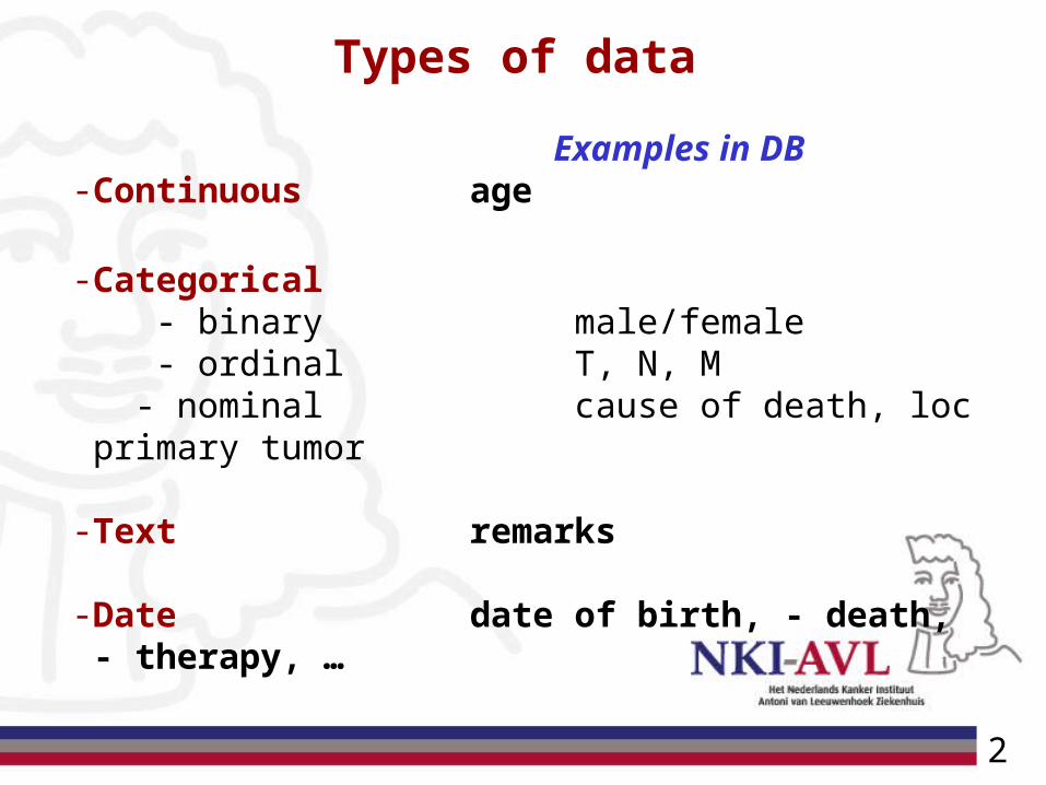
Types of data

Examples in DB- Continuous age

- Categorical - binary male/female - ordinal T, N, M - nominal cause of death, loc primary tumor

- Text remarks

- Date date of birth, - death, - therapy, …

2

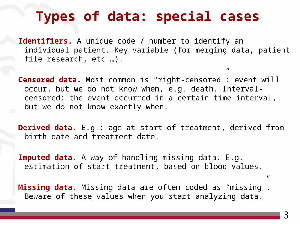
Types of data: special cases

Identifiers. A unique code / number to identify an individual patient. Key variable (for merging data, patient file research, etc …).

Censored data. Most common is “right-censored”: event will occur, but we do not know when, e.g. death. Interval-censored: the event occurred in a certain time interval, but we do not know exactly when.

Derived data. E.g.: age at start of treatment, derived from birth date and treatment date.

Imputed data. A way of handling missing data. E.g. estimation of start treatment, based on blood values.

Missing data. Missing data are often coded as “missing”. Beware of these values when you start analyzing data.

3

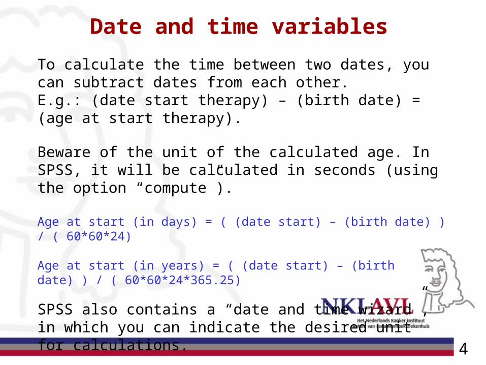
Date and time variables

To calculate the time between two dates, you can subtract dates from each other. E.g.: (date start therapy) – (birth date) = (age at start therapy).

Beware of the unit of the calculated age. In SPSS, it will be calculated in seconds (using the option “compute”).

Age at start (in days) = ( (date start) – (birth date) ) / ( 60*60*24)

Age at start (in years) = ( (date start) – (birth date) ) / ( 60*60*24*365.25)

SPSS also contains a “date and time wizard”, in which you can indicate the desired unit for calculations.

4

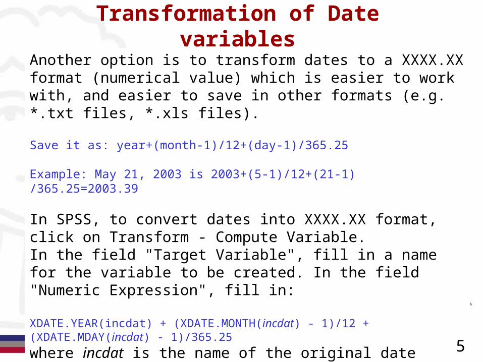
Transformation of Date variables

Another option is to transform dates to a XXXX.XX format (numerical value) which is easier to work with, and easier to save in other formats (e.g. *.txt files, *.xls files).

Save it as: year+(month-1)/12+(day-1)/365.25

Example: May 21, 2003 is 2003+(5-1)/12+(21-1) /365.25=2003.39

In SPSS, to convert dates into XXXX.XX format, click on Transform - Compute Variable. In the field "Target Variable", fill in a name for the variable to be created. In the field "Numeric Expression", fill in:

XDATE.YEAR(incdat) + (XDATE.MONTH(incdat) - 1)/12 + (XDATE.MDAY(incdat) - 1)/365.25

where incdat is the name of the original date variable.

5

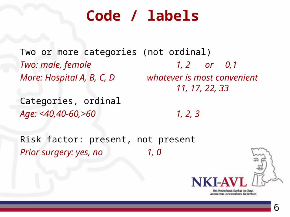
Code / labels

Two or more categories (not ordinal)Two: male, female 1, 2 or 0,1More: Hospital A, B, C, D whatever is most

convenient 11, 17, 22, 33

Categories, ordinalAge: <40,40-60,>60 1, 2, 3

Risk factor: present, not presentPrior surgery: yes, no 1, 0

6

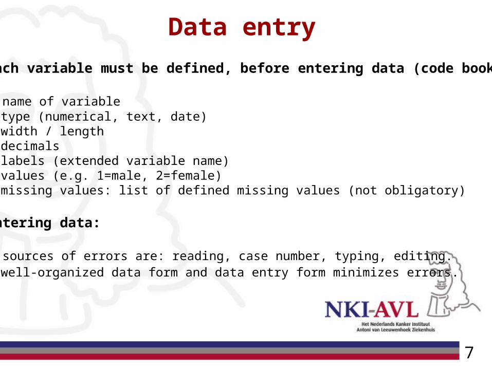
Data entry

Each variable must be defined, before entering data (code book):

- name of variable- type (numerical, text, date)- width / length- decimals- labels (extended variable name)- values (e.g. 1=male, 2=female)- missing values: list of defined missing values (not obligatory)

Entering data:

- sources of errors are: reading, case number, typing, editing.- well-organized data form and data entry form minimizes errors.

7

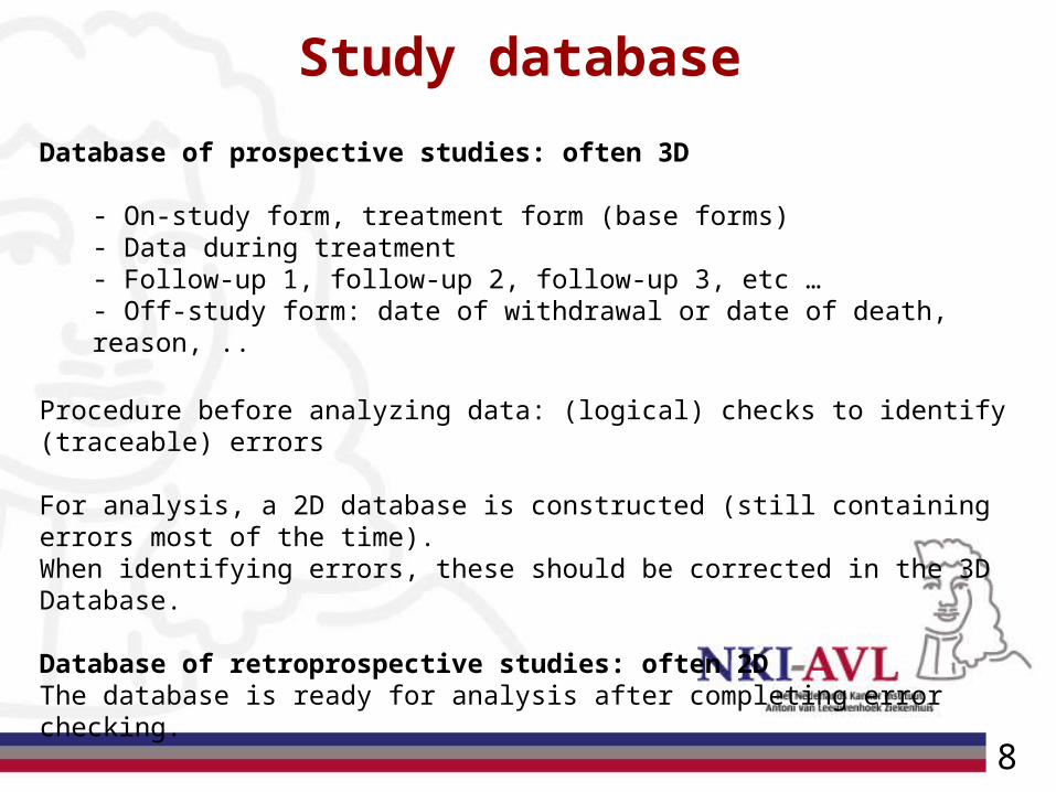
Study database

Database of prospective studies: often 3D

- On-study form, treatment form (base forms)- Data during treatment- Follow-up 1, follow-up 2, follow-up 3, etc …- Off-study form: date of withdrawal or date of death, reason, ..

Procedure before analyzing data: (logical) checks to identify (traceable) errors

For analysis, a 2D database is constructed (still containing errors most of the time).When identifying errors, these should be corrected in the 3D Database.

Database of retroprospective studies: often 2DThe database is ready for analysis after completing error checking.

8

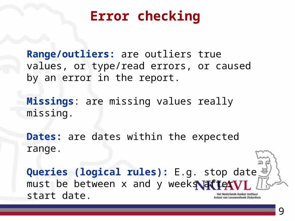
Error checking

Range/outliers: are outliers true values, or type/read errors, or caused by an error in the report.

Missings: are missing values really missing.

Dates: are dates within the expected range.

Queries (logical rules): E.g. stop date must be between x and y weeks after start date.

9

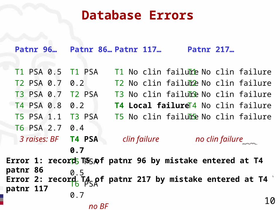
Database Errors

Patnr 96…

T1 PSA 0.5T2 PSA 0.7T3 PSA 0.7T4 PSA 0.8T5 PSA 1.1T6 PSA 2.7 3 raises: BF

Patnr 117…

T1 No clin failureT2 No clin failureT3 No clin failureT4 Local failureT5 No clin failure

clin failure

Error 1: record T5 of patnr 96 by mistake entered at T4 patnr 86Error 2: record T4 of patnr 217 by mistake entered at T4 patnr 117

Patnr 86…

T1 PSA 0.2T2 PSA 0.2T3 PSA 0.4T4 PSA 0.7T5 PSA 0.5T6 PSA 0.7 no BF

Patnr 217…

T1 No clin failureT2 No clin failureT3 No clin failureT4 No clin failureT5 No clin failure

no clin failure

10

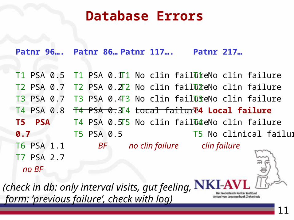
Database Errors

Patnr 96….

T1 PSA 0.5

T2 PSA 0.7

T3 PSA 0.7

T4 PSA 0.8

T5 PSA 0.7

T6 PSA 1.1

T7 PSA 2.7

no BF

Patnr 117….

T1 No clin failure

T2 No clin failure

T3 No clin failure

T4 Local failure

T5 No clin failure

no clin failure

Patnr 86…

T1 PSA 0.1

T2 PSA 0.2

T3 PSA 0.4

T4 PSA 0.3

T4 PSA 0.5

T5 PSA 0.5

BF

Patnr 217…

T1 No clin failure

T2 No clin failure

T3 No clin failure

T4 Local failure

T4 No clin failure

T5 No clinical failure

clin failure

(check in db: only interval visits, gut feeling, form: ’previous failure’, check with log)

11

Your own database

Your DB should be a transparant box, not a black box.- Keep a (short) paper file that you can consult (study forms, copies data sources,

short summaries in a Word document, …).

- Enter data preferably in a database environment (Excel: no, Access, SPSS, DBase: yes).

- Construct a code book (SPSS: labels, descriptions, and/or text file).

- Keep your original data well-organized.

- Save and backup the original data, apart from derived data / data obtained with formula’s.

- Use a text field to comment on every patient in your db, update at each update

(e.g.: “emigrated, lost f-up”, “no tox form at visit 2y”)

- Check and double-check the data.

12

Do- Throw away old databases with errors, or keep them in a

separate dir, or name them: “wrong database”.

- Add an indication of the date (e.g. sep2010) to the file name (version nr).

- Change format of a variable: first make a copy of the data column.

- … Don’t- Enter data and sort a row in Excel (it totally messes up your

database).- Rely on “file date” to know what the right database is.- Leave the database open and let computer turn in sleep mode

(hitting a key can delete data !).- …

13

2 Handling Data: descriptives & displaying dataBasic Medical Statistics CourseOctober 2010W. Heemsbergen

Describing data

To start with an extensive and good description of your data is the key to a succesful and efficient analysis of your data.

- The description of your database is needed for documentation.

- Errors can be traced more easily and at an early stage.

- You get to know your data well, which will generate good ideas about interesting analyses, as well as information about impossible analyses (e.g. too few observations per category, or too much missing data).

- You have a look-up document when you start the more complex analysis (e.g. How many patients per group were available ? Was the variable normally distributed ? Are there cases with missing values ?)

14

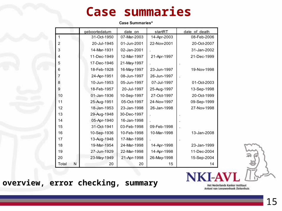
Case summaries

overview, error checking, summary

15

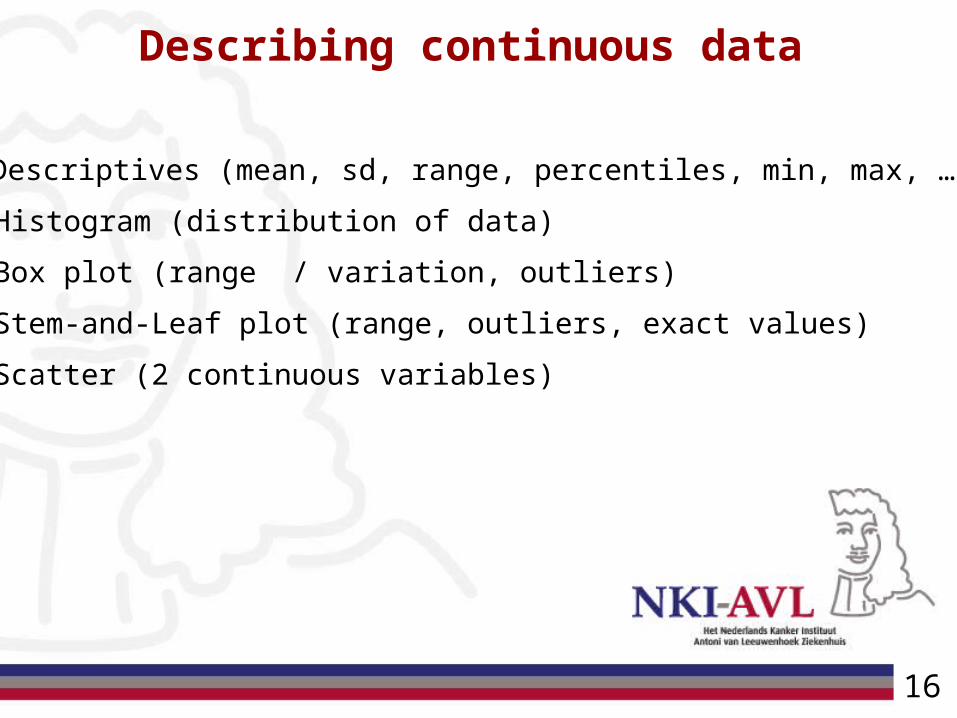
Describing continuous data

- Descriptives (mean, sd, range, percentiles, min, max, …)

- Histogram (distribution of data)

- Box plot (range / variation, outliers)

- Stem-and-Leaf plot (range, outliers, exact values)

- Scatter (2 continuous variables)

16

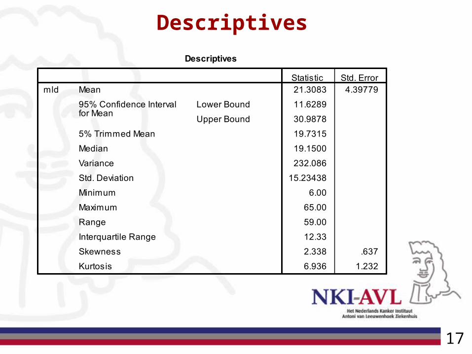
Descriptives

17

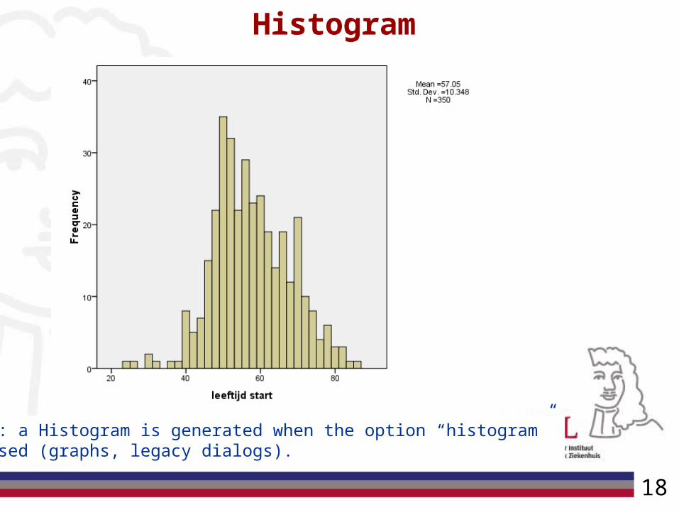
Histogram

SPSS: a Histogram is generated when the option “histogram” is used (graphs, legacy dialogs).

18

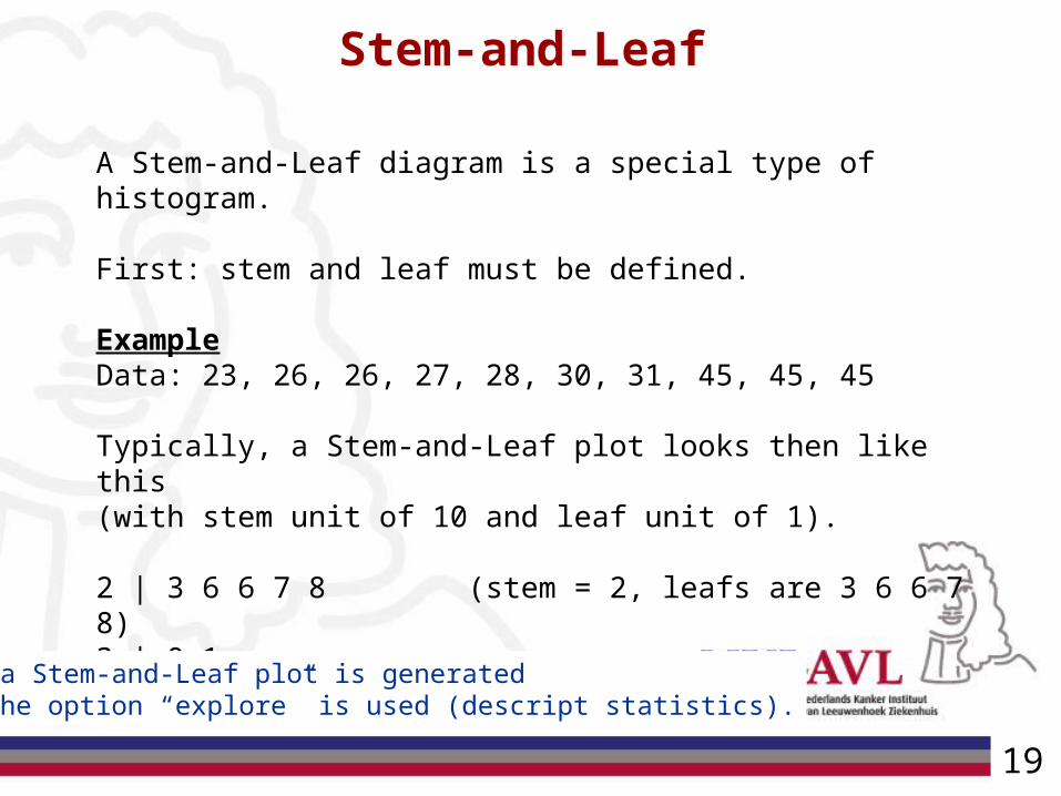
Stem-and-Leaf

A Stem-and-Leaf diagram is a special type of histogram.

First: stem and leaf must be defined.

ExampleData: 23, 26, 26, 27, 28, 30, 31, 45, 45, 45

Typically, a Stem-and-Leaf plot looks then like this (with stem unit of 10 and leaf unit of 1).

2 | 3 6 6 7 8 (stem = 2, leafs are 3 6 6 7 8)3 | 0 14 | 5 5 5

SPSS: a Stem-and-Leaf plot is generated when the option “explore” is used (descript statistics).

19

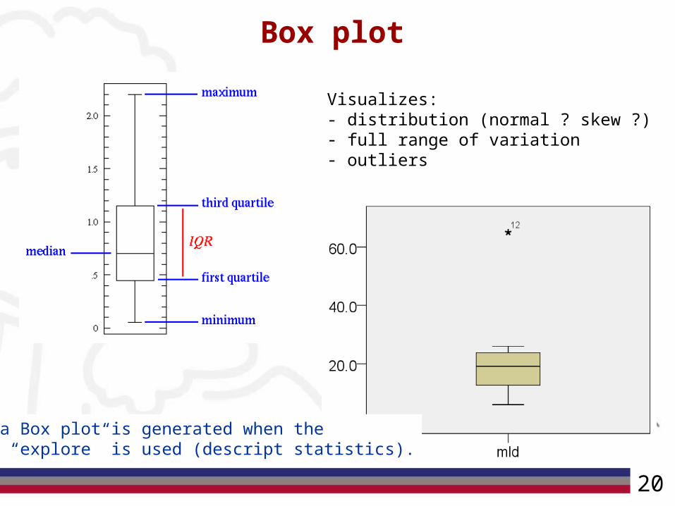
Box plot

Visualizes:- distribution (normal ? skew ?) - full range of variation - outliers

SPSS: a Box plot is generated when the option “explore” is used (descript statistics).

20

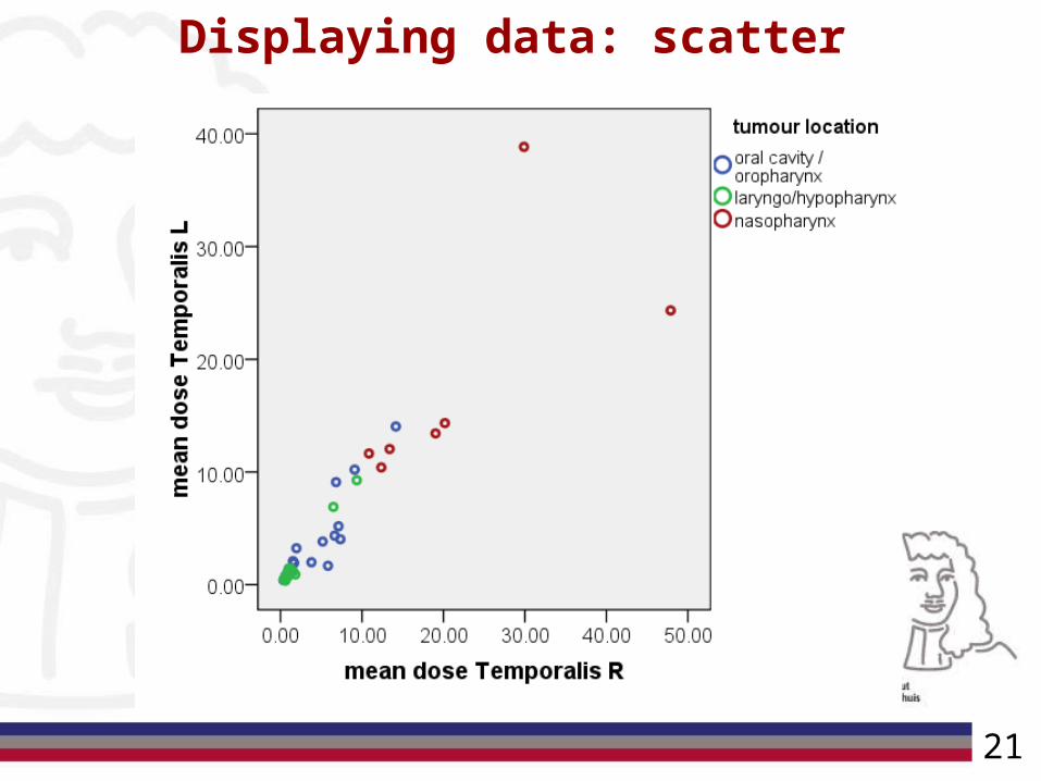
Displaying data: scatter

21

Describing categorical/ordinal data

Data can be described in absolute values (numbers) and/or in relative values (%).

Data can be described with or without missing values.

- Frequency tables- Crosstabs (at least 2 variables)- Graphs: bars, pie charts, …

22

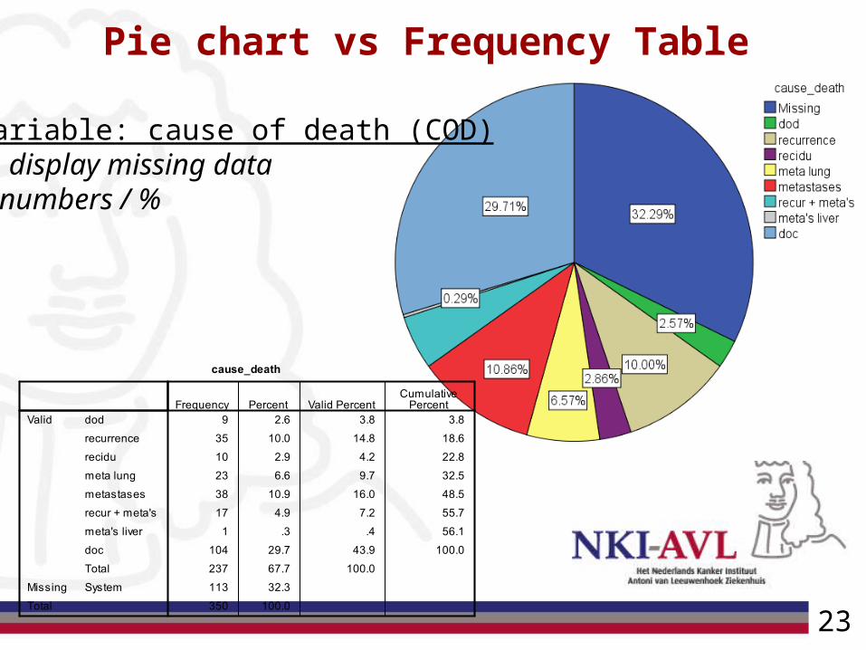
Pie chart vs Frequency Table

Variable: cause of death (COD)- display missing data- numbers / %

23

24

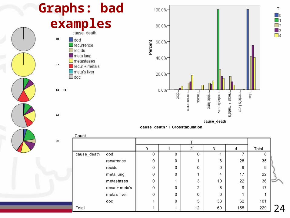
Graphs: bad examples