2. FLUID-FLOW EQUATIONS SPRING...

CFD 2 – 1 David Apsley

2. FLUID-FLOW EQUATIONS SPRING 2019

2.1 Introduction

2.2 Conservative differential equations

2.3 Non-conservative differential equations

2.4 Non-dimensionalisation

Summary

Examples

2.1 Introduction

Fluid dynamics is governed by conservation equations for:

mass;

momentum;

energy;

(for a non-homogenous fluid) other constituents.

Equations for these can be expressed mathematically as:

integral (control-volume) equations;

differential equations.

This course focuses on the control-volume approach (the basis of the finite-volume method)

because it relates naturally to physical quantities, is intrinsically conservative and is easier to

apply in modern, unstructured-mesh CFD with complex geometries. However, the equivalent

differential equations are easier to write down, manipulate and, in a few cases, solve

analytically.

Although there are many different physical quantities, most satisfy a single

generic equation: the scalar-transport or advection-diffusion equation.

(1)

The finite-volume method is a natural discretisation of this.

V


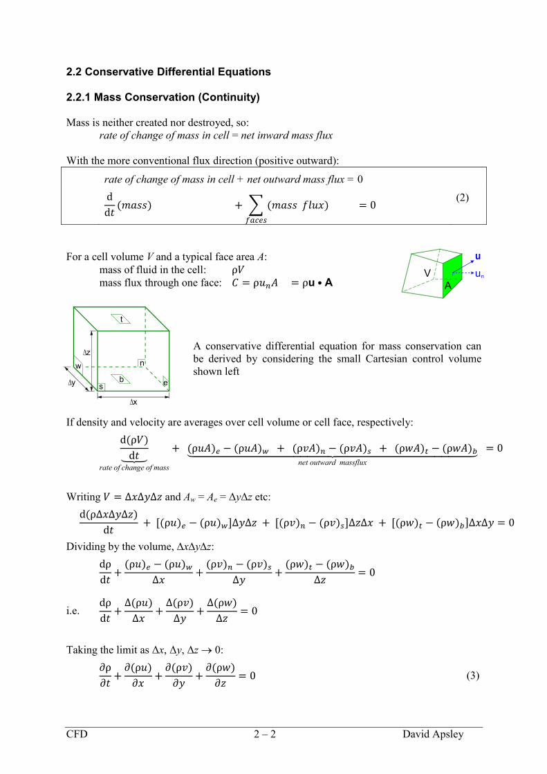
2.2 Conservative Differential Equations 2.2.1 Mass Conservation (Continuity)

Mass is neither created nor destroyed, so:

rate of change of mass in cell = net inward mass flux

With the more conventional flux direction (positive outward):

rate of change of mass in cell + net outward mass flux = 0

(2)

For a cell volume V and a typical face area A:

mass of fluid in the cell:

mass flux through one face:

A conservative differential equation for mass conservation can

be derived by considering the small Cartesian control volume

shown left

If density and velocity are averages over cell volume or cell face, respectively:

Writing and Aw = Ae = ΔyΔz etc:

Dividing by the volume, xyz:

i.e.

Taking the limit as Δx, Δy, Δz 0:

(3)

V

A

u

un

x

y

z

s e

nw

b

t


This analysis is analogous to the finite-volume procedure, but there the control volume does

not shrink to a point (finite-volume, not infinitesimal-volume) and cells can be any shape.

(*** Advanced / Optional ***)

For an arbitrary volume V with closed surface ∂V:

(4)

For a fixed control volume, take d/dt under the integral sign and apply the divergence

theorem to turn the surface integral into a volume integral:

Since V is arbitrary, the integrand must be identically zero. Hence,

(5)

Incompressible Flow

For incompressible flow, volume as well as mass is conserved, so that:

Substituting for face areas, dividing by volume and proceeding to the limit as above produces

(6)

This is usually taken as the continuity equation in incompressible flow. Note that it is

irrelevant whether the flow is time-dependent or not.


2.2.2 Momentum

Newton’s Second Law: rate of change of momentum = force

rate of change of momentum in cell + net outward momentum flux = force

(7)

For a cell volume V and a typical face area A:

momentum of fluid in the cell = mass u

momentum flux through a face =

Momentum and force are vectors, giving (in principle) 3 equations.

Fluid Forces

There are two main types:

surface forces (proportional to area; act on control-volume faces)

body forces (proportional to volume)

(i) Surface forces are usually expressed in terms of stress:

or

The main surface forces are:

pressure p: acts normal to a surface;

viscous stresses τ: frictional forces arising from relative motion.

For a simple shear flow there is only one non-zero stress component:

but, in general, τij is a symmetric tensor with a more complex

expression for its components. In incompressible flow1,

or, for a general component,

1 There is a slightly extended expression in compressible flow; see the recommended textbooks.

V

A

u

un

y

U

11

21

12

22

11

2212

x

y

21


(ii) Body forces are often expressed as forces per unit volume, or force densities.

The main body forces are:

● gravity: the force per unit volume is

(For constant-density fluids, pressure and weight can be combined as a piezometric

pressure p* = p + ρgz; gravity then no longer appears explicitly in the flow equations.)

centrifugal and Coriolis forces (apparent forces in a rotating reference frame):

centrifugal force:

Coriolis force:

Because the centrifugal force can be written as the gradient of some quantity – in this

case

– it can also be absorbed into a modified pressure and removed from the

momentum equation; see the Examples.

Differential Equation For Momentum

Consider a fixed Cartesian control volume with sides Δx, Δy, Δz. Follow

the same process as for mass conservation.

For the x-component of momentum:

Substituting cell dimensions:

Dividing by volume ΔxΔyΔz (and changing the order of pe and pw):

g

z

R

r

axis

R2

u

In inertial frame In rotating frame

x

y

z

s e

nw

b

t


In the limit as Δx, Δy, Δz 0:

(8)

Notes.

(1) The viscous term is given without proof (but see the notes below).

2 is the Laplacian operator

.

(2) The pressure force per unit volume in any direction is minus the pressure gradient in

that direction.

(3) The y and z-momentum equations can be obtained by inspection / pattern-matching.


With surface forces determined by stress tensor σij and body forces determined by force

density fi, the control-volume equation for the i component of momentum may be written

(9)

For fixed V, take d/dt inside integrals and apply the divergence theorem to surface integrals:

As V is arbitrary, the integrand vanishes identically. Hence, for arbitrary forces:

(10)

The stress tensor has pressure and viscous parts:

(11)

(12)

For a Newtonian fluid, the viscous stress tensor (including compressible part) is given by

If the fluid is incompressible and viscosity is uniform then the viscous term simplifies to give


2.2.3 General Scalar

A similar equation may be derived for any physical quantity that is advected and diffused in a

fluid flow. Examples include salt, sediment and chemical pollutants. For each such quantity

an equation is solved for the concentration (amount per unit mass of fluid) .

Diffusion causes net transport from regions of high concentration to regions of low

concentration. For many scalars this rate of transport is proportional to area and concentration

gradient and may be quantified by Fick’s diffusion law:

This is often referred to as gradient diffusion. An example is heat conduction.

For an arbitrary control volume:

amount in cell: ρV (mass concentration)

advective flux: (mass flux concentration)

diffusive flux:

(–diffusivity gradient area)

source: S = sV (source density volume)

Balancing the rate of change, the net flux through the boundary and rate of production yields

the general scalar-transport (or advection-diffusion) equation:

(13)

(Conservative) differential equation:

(14)


The integral equation may be expressed more mathematically as:

(15)

For a fixed control volume, taking the time derivative under the integral sign and using the

divergence theorem gives a corresponding conservative differential equation:

(16)

V

A

u

un


2.2.4 Momentum Components as Transported Scalars

In the momentum equation, if the viscous force is transferred to the LHS it

looks like a diffusive flux. For example, for the x-component:

Compare this with the generic scalar-transport equation:

Each component of momentum satisfies its own scalar-transport equation, with

concentration, velocity component (u, v or w)

diffusivity, Γ viscosity μ

source, S other forces

Consequently, only one generic scalar-transport equation need be considered.

In Section 5 we shall see, however, that the momentum components differ from passive

scalars (those not affecting the flow), because:

equations are nonlinear (mass flux involves the velocity component being solved for);

equations are coupled (mass flux involves the other velocity components as well);

the velocity field must also be mass-consistent.

2.2.5 Non-Gradient Diffusion

The analysis above assumes that all non-advective flux is simple gradient diffusion:

Actually, the real situation is more complex. For example, in the u-momentum equation the

full expression for the 1-component of viscous stress through the 2-face is

The ∂u/∂y part is gradient diffusion of u, but the ∂v/∂x term is not. In general, non-advective

fluxes that can’t be represented by gradient diffusion are discretised conservatively (i.e.

worked out for cell faces, not particular cells), then transferred to the RHS as a source term:


2.2.6 Moving Control Volumes

Control-volume equations are also applicable to moving control volumes, provided the

normal velocity component in the mass flux is that relative to the mesh; i.e.

The finite-volume method can thus be used for calculating flows with moving boundaries2.

2.3 Non-Conservative Differential Equations

Conservative differential equations are so-called because they can be integrated directly to

give an equivalent integral form involving the net change in a flux, with the flux leaving one

cell equal to that entering an adjacent cell. To do so, all terms involving derivatives of

dependent variables must have differential operators “on the outside”. In one dimension:


The three-dimensional version uses partial derivatives and the divergence theorem to change

the differentials to surface flux integrals.

As an example of how the same equation can appear in conservative and non-conservative

forms, consider a simple 1-d example:

(conservative form – can be integrated directly)

(non-conservative form, obtained by applying the chain rule)

Material Derivatives

The time rate of change of some property in a fluid element moving with the flow is called

the material (or substantive) derivative. It is denoted by D/Dt and defined below.

Every field variable is a function of both time and position; i.e.

As one follows a path through space, changes with time because:

it changes with time t at each point; and

it changes with position (x, y, z) as it moves with the flow.

2 See, for example: Apsley, D.D. and Hu, W., 2003, CFD Simulation of two- and three-dimensional free-surface

flow, International Journal for Numerical Methods in fluids, 42, 465-491.

(x(t), y(t), z(t))


Thus, the total time derivative following an arbitrary path (x(t), y(t), z(t)) is

The material derivative is the time derivative along the particular path following the flow

(dx/dt = u, etc.):

or

(17)

In particular, the material derivative of velocity (Du/Dt) is the acceleration (Hydraulics 1).

For general scalar , the sum of time-dependent and advection terms (total rate of change) is

(by the product rule)

(18)

Using the material derivative, a scalar-transport equation can thus be written in a much more

compact, but non-conservative, form. In particular, the momentum equation becomes

(19)

This form is much simpler to write and is used both for convenience and to derive theoretical

results in special cases (see the Examples). However, in the finite-volume method it is the

longer, conservative form which is actually discretised.



The derivation of (18) above is greatly simplified by use of the summation convention:

or vector derivatives:

Alternatively, conservative differential equations may derived from fixed control volumes

(Eulerian approach) and their non-conservative counterparts from control volumes moving

with the flow (Lagrangian approach).


2.4 Non-Dimensionalisation

Although it is possible to work entirely in dimensional quantities, there are good theoretical

reasons for working in non-dimensional variables. These include the following.

All dynamically-similar problems (same Re, Fr etc.) can be solved with a single

computation.

The number of relevant parameters (and hence the number of graphs needed to report

results) is reduced.

It indicates the relative size of different terms in the governing equations and, in

particular, which might conveniently be neglected.

Computational variables are of a similar order of magnitude (ideally, of order unity),

yielding better numerical accuracy.

2.4.1 Non-Dimensionalising the Governing Equations

For incompressible flow the governing equations are:

continuity:

(20)

momentum:

(21)

(and similar in y, z directions)

Adopting reference scales U0, L0 and ρ0 for velocity, length and density, respectively, and

derived scales L0/U0 for time and for pressure, each fluid quantity can be written as a

product of a dimensional scale and a non-dimensional variable (indicated by a *):

Substituting into mass and momentum equations (20) and (21) yields, after simplification:

(22)

where

(23)

From this, it is seen that the key dimensionless group is the Reynolds number Re. If Re is

large then viscous forces would be expected to be negligible in much of the flow.

Having derived the non-dimensional equations it is usual to drop the asterisks and simply

declare that you are “working in non-dimensional variables”.


Note.

The objective is that non-dimensional quantities (e.g. p*) should be order of

magnitude unity, so the scale for a quantity should reflect its range of values, not

necessarily its absolute value. In incompressible (but not compressible) flow it is

differences in pressure that are important, not absolute values. Since flow-induced

pressures are usually much smaller than the absolute pressure, one usually works with

departures from a constant reference pressure pref and use as a scale magnitude;

Hence, we non-dimensionalise as: .

Similarly, in Section 3 when we look at small changes in density due to temperature

or salinity that give rise to buoyancy forces we shall use an alternative non-

dimensionalisation:

(24)

with Δρ the overall size of density variation and θ* typically varying between 0 and 1.

2.4.2 Common Dimensionless Groups

If other types of fluid force are included then each introduces another non-dimensional group.

For example, gravitational forces lead to a Froude number (Fr) and Coriolis forces to a

Rossby number (Ro). Some of the most important dimensionless groups are given below. U

and L are representative velocity and length scales, respectively.

Reynolds number (viscous flow; μ = dynamic viscosity)

Froude number (open-channel flow; g = gravity)

Mach number (compressible flow; c = speed of sound)

Rossby number (rotating flows; Ω = angular velocity of frame)

Weber number (interfacial flows; σ = surface tension)

Note.

For flows with buoyancy forces caused by a change in density, rather than open-channel

flows, we sometimes use a densimetric Froude number instead; this is defined by

Here, g is replaced in the usual formula for Froude number by , sometimes called the

reduced gravity g: see Section 3.


Summary

Fluid dynamics is governed by conservation equations for mass, momentum, energy

(and, for a non-homogeneous fluid, the amount of individual constituents).

The governing equations can be written in equivalent integral (control-volume) or

differential forms.

The finite-volume method is a direct discretisation of the control-volume equations.

Differential forms of the flow equations may be conservative (i.e. can be integrated

directly to something of the form “fluxout – fluxin = source”) or non-conservative.

For any conserved quantity and arbitrary control volume:

rate of change + net outward flux = source

There are really just two canonical equations to discretise and solve:

mass conservation (continuity):

scalar-transport (or advection-diffusion) equation:

Each velocity component (u, v, w) satisfies its own scalar-transport equation.

However, these equations differ from those for a passive scalar because they are non-

linear, coupled through the advective fluxes and pressure forces, and the velocity field

is also required to be mass-consistent.

Non-dimensionalising the governing equations allows dynamically-similar flows

(those with the same values of Reynolds number, etc.) to be solved with a single

calculation, reduces the overall number of parameters, indicates whether certain terms

in the governing equations are significant or negligible and ensures that the main

computational variables are of similar magnitude.


Examples

Q1.

In 2-d flow, the continuity and x-momentum equations can be written in conservative form as

respectively.

(a) Show that these can be written in the equivalent non-conservative forms:

where the material derivative is given (in 2 dimensions) by

.

(b) Define carefully what is meant by the statement that a flow is incompressible. To

what does the continuity equation reduce in incompressible flow?

(c) Write down conservative forms of the 3-d equations for mass and x-momentum.

(d) Write down the z-momentum equation, including the gravitational force.

(e) Show that, for constant-density flows, pressure and gravity forces can be combined in

the momentum equations via the piezometric pressure p + ρgz.

(f) In a rotating reference frame there are additional apparent forces (per unit volume):

centrifugal force: or

Coriolis force:

where is the angular velocity of the reference frame, u is the

fluid velocity in that frame, r is the position vector (relative to a

point on the axis of rotation) and R is its projection perpendicular

to the axis of rotation. ( denotes vector product.)

By writing the centrifugal force as the gradient of some quantity

show that it can be subsumed into a modified pressure. Also, find

the components of the Coriolis force if rotation is about the z axis.


(g) Write the conservative mass and momentum equations in vector notation.

(h) Write the conservative mass and momentum equations in suffix notation using the

summation convention.

R

r

axis

R2


Q2. (Exact solutions of the Navier-Stokes equation)

The x-component of the momentum equation is given by

Using this equation derive the velocity profile in fully-developed, laminar flow for:

(a) pressure-driven flow between stationary parallel planes (“Plane Poiseuille flow”);

(b) constant-pressure flow between stationary and moving planes (“Couette flow”).

Assume flow in the x direction, with bounding planes y = 0

and y = h. The velocity is then (u(y),0,0). In part (a) both walls

are stationary. In part (b) the upper wall slides parallel to the

lower wall with velocity Uw.

(c) (*** Advanced / Optional ***) In cylindrical polars (x,r,) the Laplacian 2 is more

complicated. If axisymmetric, with fully-developed velocity , then

Derive the velocity profile in a circular pipe with stationary wall at r = R (“Poiseuille flow”).

Q3. (*** Advanced / Optional ***)

By applying the divergence theorem, deduce the conservative and non-conservative

differential equations corresponding to the general integral scalar-transport equation

Q4.

In each of the following cases, state which of (i), (ii), (iii) is a valid dimensionless number.

Carry out research to find the name and physical significance of these numbers.

(L = length; U = velocity; z = height; p = pressure; ρ = density; μ = dynamic viscosity;

ν = kinematic viscosity; g = gravitational acceleration; Ω = angular velocity).

(a) (i)

(ii)

(iii)

(b) (i)

(ii)

(iii)

(c) (i)

(ii)

(iii)

(d) (i)

(ii)

(iii)

u(y) hy

x


Q5. (Exam 2008; part (h) depends on later sections of this course)

The momentum equation for a viscous fluid in a rotating reference frame is

(*)

where ρ is density, u = (u,v,w) is velocity, p is pressure, μ is dynamic viscosity and is the

angular-velocity vector of the reference frame. The symbol denotes a vector product.

(a) If write down the x and y components of the Coriolis force ( ).

(b) Hence write down the x- and y-components of equation (*).

(c) Show how Equation (*) can be written in non-dimensional form in terms of a

Reynolds number Re and Rossby number Ro (both of which should be defined).

(d) Define the terms conservative and non-conservative when applied to the differential

equations describing fluid flow.

(e) Define (mathematically) the material derivative operator D/Dt. Then, noting that the

continuity equation can be written

show that the x-momentum equation can be written in an equivalent conservative

form.

(f) If the x-momentum equation were to be regarded as a special case of the general

scalar-transport (or advection-diffusion) equation, identify the quantities representing:

(i) concentration;

(ii) diffusivity;

(iii) source.

(g) Explain why the three equations for the components of momentum cannot be treated

as independent scalar equations.

(h) Explain (briefly) how pressure is determined in a CFD simulation of:

(i) high-speed, compressible gas flow;

(ii) incompressible flow.


Q6.

(a) In a rotating reference frame (with angular velocity vector ) the non-viscous forces

on a fluid are, per unit volume,

where p is pressure, g = (0,0,–g) is the gravity vector and R is the vector from the

closest point on the axis of rotation to a point. Show that, in a constant-density fluid,

force densities (I), (II) and (III) can be combined in terms of a modified pressure.

(b) Consider a closed cylindrical can of radius 5 cm and depth 15 cm. The can is

completely filled with fluid of density 1100 kg m–3

and is rotating steadily about its

axis (which is vertical) at 600 rpm. Where do the maximum and minimum pressures

in the can occur, and what is the difference in pressure between them?

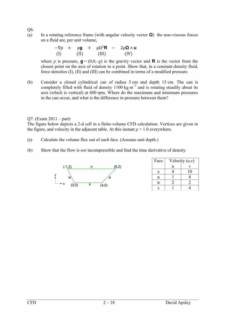
Q7. (Exam 2011 – part)

The figure below depicts a 2-d cell in a finite-volume CFD calculation. Vertices are given in

the figure, and velocity in the adjacent table. At this instant ρ = 1.0 everywhere.

(a) Calculate the volume flux out of each face. (Assume unit depth.)

(b) Show that the flow is not incompressible and find the time derivative of density.

Face Velocity (u,v)

u v

e 4 10

n 1 8

w 2 2

s 1 4

e

s

w

n

(4,0)

(6,2)(-1,2)

(0,0)x

y

2. FLUID-FLOW EQUATIONS SPRING...

Documents

Transcript of 2. FLUID-FLOW EQUATIONS SPRING...