2-d nozzle_cfd

problems the pressure and velocity fields are coupled, so the pressure correction equation must be solved along with the discretised momentumequations. Furthermore, we note that the value of d in expression (6.59) forthe velocity corrections was assumed to be constant. Normally, the value ofd will vary from node to node and must be calculated with (6.23) and (6.28)using control volume face areas and central coefficient (aP) values from thediscretised momentum equations. This process will be illustrated in the nextexample.

A planar two-dimensional nozzle is shown in Figure 6.10. The flow is steadyand frictionless and the density of the fluid is constant.

200 CHAPTER 6 ALGORITHMS FOR PRESSURE---VELOCITY COUPLING

Figure 6.10 Geometry of planar2D nozzle

Figure 6.11 (a) The grid forpressure control volumes; (b) thegrid for velocity control volumes

Example 6.2

Use the backward-staggered grid with five pressure nodes and four velocity nodes shown in Figures 6.11a–b. The stagnation pressure is given atthe inlet and the static pressure is specified at the exit. Using the SIMPLE

ANIN_C06.qxd 29/12/2006 09:59 AM Page 200

6.10 WORKED EXAMPLES OF THE SIMPLE ALGORITHM 201

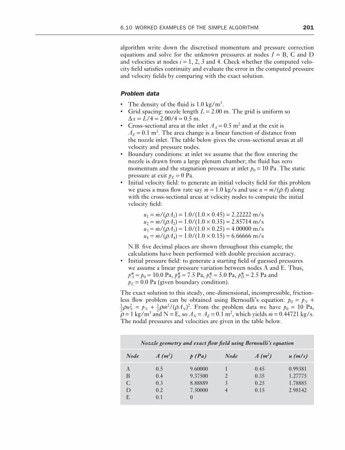
algorithm write down the discretised momentum and pressure correctionequations and solve for the unknown pressures at nodes I = B, C and D and velocities at nodes i = 1, 2, 3 and 4. Check whether the computed velo-city field satisfies continuity and evaluate the error in the computed pressureand velocity fields by comparing with the exact solution.

Problem data

• The density of the fluid is 1.0 kg/m3.• Grid spacing: nozzle length L = 2.00 m. The grid is uniform so

∆x = L/4 = 2.00/4 = 0.5 m.• Cross-sectional area at the inlet AA = 0.5 m2 and at the exit is

AE = 0.1 m2. The area change is a linear function of distance from the nozzle inlet. The table below gives the cross-sectional areas at allvelocity and pressure nodes.

• Boundary conditions: at inlet we assume that the flow entering thenozzle is drawn from a large plenum chamber; the fluid has zeromomentum and the stagnation pressure at inlet p0 = 10 Pa. The staticpressure at exit pE = 0 Pa.

• Initial velocity field: to generate an initial velocity field for this problemwe guess a mass flow rate say K = 1.0 kg/s and use u = K/(ρA) alongwith the cross-sectional areas at velocity nodes to compute the initialvelocity field:

u1 = K/(ρA1) = 1.0/(1.0 × 0.45) = 2.22222 m/su2 = K/(ρA2) = 1.0/(1.0 × 0.35) = 2.85714 m/su3 = K/(ρA3) = 1.0/(1.0 × 0.25) = 4.00000 m/su4 = K/(ρA4) = 1.0/(1.0 × 0.15) = 6.66666 m/s

N.B. five decimal places are shown throughout this example; thecalculations have been performed with double precision accuracy.

• Initial pressure field: to generate a starting field of guessed pressures we assume a linear pressure variation between nodes A and E. Thus, p*A = p0 = 10.0 Pa, p*B = 7.5 Pa, p*C = 5.0 Pa, p*D = 2.5 Pa and pE = 0.0 Pa (given boundary condition).

The exact solution to this steady, one-dimensional, incompressible, friction-less flow problem can be obtained using Bernoulli’s equation: p0 = pN +1–2ρu2

N = pN + 1–2ρK2/(ρAN)2. From the problem data we have p0 = 10 Pa,

ρ = 1 kg/m3 and N = E, so AN = AE = 0.1 m2, which yields K = 0.44721 kg/s.The nodal pressures and velocities are given in the table below.

Nozzle geometry and exact flow field using Bernoulli’s equation

Node A (m2) p (Pa) Node A (m2) u (m/s)

A 0.5 9.60000 1 0.45 0.99381B 0.4 9.37500 2 0.35 1.27775C 0.3 8.88889 3 0.25 1.78885D 0.2 7.50000 4 0.15 2.98142E 0.1 0

ANIN_C06.qxd 29/12/2006 09:59 AM 01


The governing equations for steady, one-dimensional, incompressible, fric-tionless equations through the planar nozzle are as follows:

Mass conservation: (ρAu) = 0 (6.61)

Momentum conservation: ρuA = −A (6.62)

These equations are familiar from introductory fluid mechanics texts. Aderivation has also been given in Appendix E.

Discretised u-momentum equation

The discretised form of momentum equation (6.62) is

(ρuA)e ue − (ρuA)w uw = ∆V

where the right hand side represents the pressure gradient integrated overthe control volume ∆V and ∆p = pw − pe.

In standard notation the discretised momentum equation for this one-dimensional problem can be written as

aP u*P = aW u*W + aE u*E + Su

If we use the upwind differencing scheme the coefficients may beobtained from (see Section 5.6)

aW = Dw + max(Fw, 0)aE = De + max(0, −Fe)aP = aW + aE + (Fe − Fw)

The flow is frictionless so there is no viscous diffusion term in the governingequation, and hence Dw = De = 0. Fw and Fe are mass flow rates through thewest and east faces of the u-control volume. We compute the face velocitiesneeded for Fw and Fe from averages of velocity values at nodes straddling the face and use the correct values of the west and east face area given in the above table. At the start of the calculations we use the initial velocity field generated from the guessed mass flow rate. For subsequent iterationswe use the corrected velocity obtained after solving the pressure correctionequation.

The source term Su contains the pressure gradient integrated over thecontrol volume:

Su = × ∆V = × Aav∆x = ∆p × (Aw + Ae)

Since the geometry has a varying cross-sectional area we use an averaged areato calculate ∆V. At first glance this looks like a very crude approximation,but it is possible to show that the accuracy order of Su is no worse than theupstream differencing used for the momentum flux terms.

In summary the coefficients of the discretised u-equations are given by

Fw = ρAw uw and Fe = ρAe ueaW = FwaE = 0

1

2

∆p

∆x

∆p

∆x

∆p

∆x

dp

dx

du

dx

d

dx

Solution

ANIN_C06.qxd 29/12/2006 09:59 AM Page 202


aP = aW + aE + (Fe − Fw)Su = ∆p × 1–

2(Aw + Ae) = ∆p × AP

The parameter d required in the pressure correction equations is calculatedat this stage from

d = =

Pressure correction equation

The discretised form of the continuity equation in this one-dimensionalgeometry is

(ρuA)e − (ρuA)w = 0

The corresponding pressure correction equation is

aP p ′P = aW p ′W + aE p ′E + b′

where aW = (ρdA)w, aE = (ρdA)eb ′ = (F *w − F *e )

Values of the parameter d come from discretised momentum equations (seeabove and Section 6.4).

In the SIMPLE algorithm the pressure corrections p′ are used to computethe velocity corrections u′ and the corrected pressure and velocity fields using

u′ = d (p ′I − p ′I+1)

p = p* + p′u = u* + u′

Numerical values --- momentum equation

First we consider the internal nodes 2 and 3.

• Velocity node 2

Fw = (ρuA)w = 1.0 × [(u1 + u2)/2] × 0.4 = 1.0 × [(2.2222 + 2.8571)/2] × 0.4 = 1.01587

Fe = (ρuA)e = 1.0 × [(u2 + u3)/2] × 0.3 = 1.0 × [(2.8571 + 4.0)/2] × 0.3 = 1.02857

aW = Fw = 1.01587

aE = 0

aP = aW + aE + (Fe − Fw) = 1.01587 + 0 + (1.02857 − 1.01587) = 1.02857

Su = ∆P × A2 = (pB − pC) × A2 = (7.5 − 5.0) × 0.35 = 0.875

The discretised momentum equation at node 2 is

1.02857u2 = 1.01587u1 + 0.875

We also need to calculate the parameter d at this node for later use inthe pressure correction equation:

d2 = A2/aP = 0.35/1.02857 = 0.34027

(Aw + Ae)

2aP

Aav

aP

ANIN_C06.qxd 29/12/2006 09:59 AM Page 203

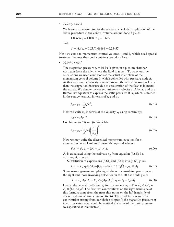
• Velocity node 3

We leave it as an exercise for the reader to check that application of theabove procedure at the control volume around node 3 yields

1.06666u3 = 1.02857u2 + 0.625

and

d3 = A3/aP = 0.25/1.06666 = 0.23437

Next we come to momentum control volumes 1 and 4, which need specialtreatment because they both contain a boundary face.

• Velocity node 1

The stagnation pressure p0 = 10 Pa is given in a plenum chamberupstream from the inlet where the fluid is at rest. To carry out thecalculations we need conditions at the actual inlet plane of themomentum control volume 1, which coincides with pressure node A. At this location the velocity is non-zero and the actual pressure is lowerthan the stagnation pressure due to acceleration of the flow as it entersthe nozzle. We denote the (as yet unknown) velocity at A by uA and useBernoulli’s equation to express the static pressure at A, which is neededin the source term Su, in terms of p0 and uA:

pA = p0 − (ρu 2A) (6.63)

Next we write uA in terms of the velocity u1 using continuity:

uA = u1A1/AA (6.64)

Combining (6.63) and (6.64) yields

pA = p0 − ρu 21

2

(6.65)

Now we may write the discretised momentum equation for u-momentum control volume 1 using the upwind scheme:

Fe u1 − Fw uA = (pA − pB) × A1 (6.66)

Fw is calculated using the estimate uA from equation (6.64): i.e. Fw = ρuA AA = ρu1A1.

Substitution of expressions (6.64) and (6.65) into (6.66) gives

Fe u1 − Fw u1A1/AA =[(p0 − 1–2ρu 2

1(A1/AA)2) − pB] × A1 (6.67)

Some rearrangement and placing all the terms involving pressures onthe right and those involving velocities on the left hand side yields

[Fe − Fw A1/AA + Fw × 1–2(A1/AA)2]u1 = (p0 − pB)A1 (6.68)

Hence, the central coefficient aP for this node is aP = Fe − Fw A1/AA +Fw × 1–

2(A1/AA)2. The first two contributions on the right hand side of

this formula come from the mass flux terms on the left hand side ofdiscretised momentum equation (6.66). The third term is an extracontribution arising from our choice to specify the stagnation pressure atinlet (this extra term would be omitted if a value of the static pressurewas specified at inlet instead).

DEF

A1

AA

ABC

1

2

1

2


ANIN_C06.qxd 29/12/2006 09:59 AM Page 204


Expression (6.68) can be used in that form, but in these calculationswe have chosen to place the negative contribution to coefficient a1 onthe right hand side. Hence

[Fe + Fw × 1–2(A1/AA)2]u1 = (p0 − pB)A1 + Fw A1/AA × u old

1(6.69)

where u1old is the nodal velocity at the previous iteration

This is termed the deferred correction approach and can be effective instabilising the iterative process if the initial velocity field is based on avery poor guess (see also Chapter 5 – QUICK and TVD).

Now we calculate

uA = u1A1/AA = 2.22222 × 0.45/0.5 = 2.0

Fw = (ρuA)w = ρuAAA = 1.0 × 2.0 × 0.5 = 1.0

The exit mass flux Fe is computed in the same way as for the internalnodes:

Fe = (ρuA)e = 1.0 × [(u1 + u2)/2] × 0.4 = 1.0 × [(2.2222 + 2.8571)/2] × 0.4 = 1.01587

aW = 0

aE = 0

aP = Fe + Fw × 1–2(A1/AA)2 = 1.01587 + 1.0 × 0.5 × (0.45/0.5)2

= 1.42087

In the source term we apply p0 = 10 Pa and the initial velocity u

1old = 2.22222 m/s.

Su = (p0 − pB)A1 + Fw(A1/AA) × u1old

= (10 − 7.5) × 0.45 + 1.0 × (0.45/0.5) × 2.22222= 3.125

The discretised momentum equation at node 1 is therefore

1.42087u1 = 3.125

The parameter d at this node is

d1 = A1/aP = 0.45/1.4209 = 0.31670

• Velocity node 4

Fw = (ρuA)w = 1.0 × [(u3 + u4)/2] × 0.2 = 1.06666

At the east boundary of momentum control volume 4 we have a fixedpressure, but we do not have two velocities that straddle the eastboundary. To compute the mass flux across this boundary we imposecontinuity:

Fe = (ρuA)4

At the first iteration we can use the assumed mass flow rate, so we set Fe = 1.0 kg/s. Thus,

aW = Fw = 1.06666aE = 0aP = aW + aE + (Fe − Fw) = 1.06666 + 0 + (1.0 − 1.06666) = 1.0

ANIN_C06.qxd 29/12/2006 09:59 AM Page 205


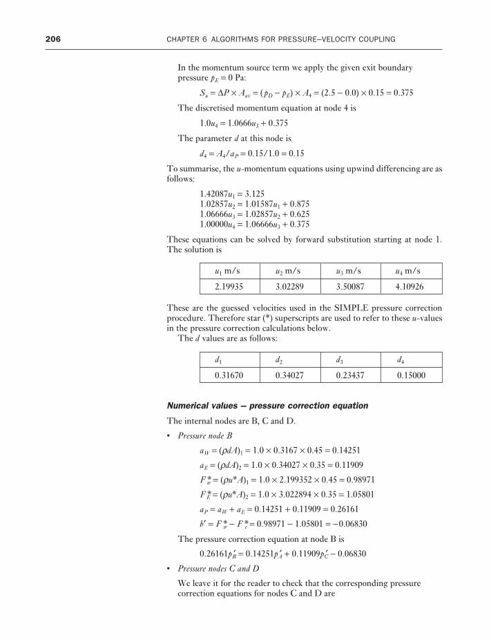
In the momentum source term we apply the given exit boundarypressure pE = 0 Pa:

Su = ∆P × Aav = (pD − pE) × A4 = (2.5 − 0.0) × 0.15 = 0.375

The discretised momentum equation at node 4 is

1.0u4 = 1.0666u3 + 0.375

The parameter d at this node is

d4 = A4/aP = 0.15/1.0 = 0.15

To summarise, the u-momentum equations using upwind differencing are asfollows:

1.42087u1 = 3.1251.02857u2 = 1.01587u1 + 0.8751.06666u3 = 1.02857u2 + 0.6251.00000u4 = 1.06666u3 + 0.375

These equations can be solved by forward substitution starting at node 1.The solution is

u1 m/s u2 m/s u3 m/s u4 m/s

2.19935 3.02289 3.50087 4.10926

These are the guessed velocities used in the SIMPLE pressure correctionprocedure. Therefore star (*) superscripts are used to refer to these u-valuesin the pressure correction calculations below.

The d values are as follows:

d1 d2 d3 d4

0.31670 0.34027 0.23437 0.15000

Numerical values --- pressure correction equation

The internal nodes are B, C and D.

• Pressure node B

aW = (ρdA)1 = 1.0 × 0.3167 × 0.45 = 0.14251

aE = (ρdA)2 = 1.0 × 0.34027 × 0.35 = 0.11909

F *w = (ρu*A)1 = 1.0 × 2.199352 × 0.45 = 0.98971

F *E = (ρu*A)2 = 1.0 × 3.022894 × 0.35 = 1.05801

aP = aW + aE = 0.14251 + 0.11909 = 0.26161

b′ = F *w − F *e = 0.98971 − 1.05801 = −0.06830

The pressure correction equation at node B is

0.26161p ′B = 0.14251p ′A + 0.11909p ′C − 0.06830

• Pressure nodes C and D

We leave it for the reader to check that the corresponding pressurecorrection equations for nodes C and D are

ANIN_C06.qxd 29/12/2006 09:59 AM Page 206


0.17769p ′C = 0.11909p ′B + 0.058593p ′D + 0.18279

0.081093p ′D = 0.058593p ′C + 0.02249p ′E + 0.25882

Nodes are A and E are boundary nodes so they need special treatment.

• Pressure nodes A and E

The pressure corrections are set to zero for both nodes:

p ′A = 0.0

p ′E = 0.0

At node E this follows the practice of Example 6.1, because the staticpressure is given at the nozzle exit. If the static pressure pA at inlet wasgiven this would also apply at node A without reservation. However, inthis problem we are working with a given stagnation pressure, so weneed to be careful. We note that pA is fixed by Equation (6.65) if thestagnation pressure p0 and velocity u1 are known. At the stage in theSIMPLE algorithm where we start to solve the pressure correctionequations, we have available the guessed velocity u*1 as a result of solvingthe discretised momentum equation. Whilst it is true that this velocity isconstantly updated as the iterations proceed, we may regard that at eachiteration level the static pressure pA is temporarily fixed by p0 and thecurrent value of u*1, thus justifying the use of p ′A = 0.0.

Substitution of p ′A = 0.0 and p ′E = 0.0 into the pressure correction equationsfor internal nodes B, C and D yields the following system of equations:

0.26161p ′B = 0.11909p ′C − 0.06830

0.17769p ′C = 0.11909p ′B + 0.058593p ′D + 0.18279

0.081093p ′D = 0.058593p ′C + 0.25882

These three equations can be solved to give the pressure correction at nodesB, C and D. The resulting solution is

p ′A p ′B p ′C p ′D p ′E0.0 1.63935 4.17461 6.20805 0.0

Corrected nodal pressures are now calculated using these pressure corrections:

pB = p*B + p ′B = 7.5 + 1.63935 = 9.13935

pC = p*C + p ′C = 5.0 + 4.17461 = 9.17461

pD = p*D + p ′D = 2.5 + 6.20805 = 8.70805

Corrected velocities at the end of the first iteration are

u1 = u*1 + d1(p ′A − p ′B) = 2.19935 + 0.31670 × [0.0 − 1.63935] = 1.68015 m/s

u2 = u*2 + d2(p ′B − p ′C) = 3.02289 + 0.34027 × [1.63935 − 4.17461] = 2.16020 m/s

u3 = u*3 + d3(p ′C − p ′D) = 3.50087 + 0.23437 × [4.17461 − 6.20805] = 3.02428 m/s

u4 = u*4 + d4(p ′D − p ′E) = 4.10926 + 0.15 × [6.20805 − 0.0] = 5.04047 m/s

We can also calculate the corrected nodal pressure at A using equation (6.65):

pA = p0 − 1–2ρu 2

1 (A1/AA)2 = 10 − 1–2

× 1.0 × (1.68015 × 0.45/0.5)2 = 8.85671

ANIN_C06.qxd 29/12/2006 09:59 AM Page 207


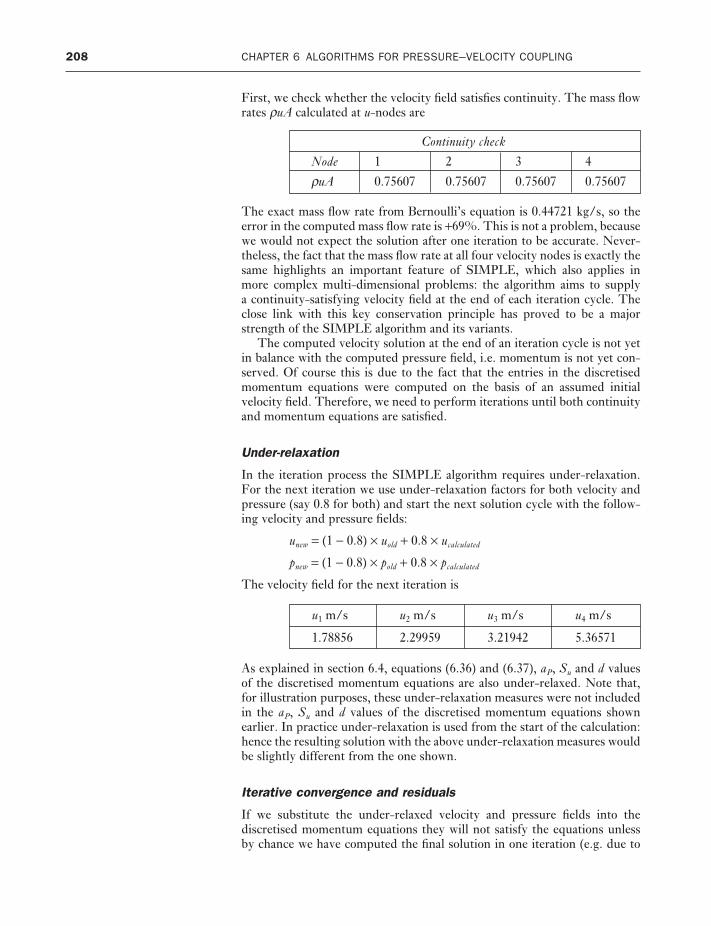
First, we check whether the velocity field satisfies continuity. The mass flowrates ρuA calculated at u-nodes are

Continuity check

Node 1 2 3 4

ρuA 0.75607 0.75607 0.75607 0.75607

The exact mass flow rate from Bernoulli’s equation is 0.44721 kg/s, so theerror in the computed mass flow rate is +69%. This is not a problem, becausewe would not expect the solution after one iteration to be accurate. Never-theless, the fact that the mass flow rate at all four velocity nodes is exactly thesame highlights an important feature of SIMPLE, which also applies in more complex multi-dimensional problems: the algorithm aims to supply a continuity-satisfying velocity field at the end of each iteration cycle. Theclose link with this key conservation principle has proved to be a majorstrength of the SIMPLE algorithm and its variants.

The computed velocity solution at the end of an iteration cycle is not yetin balance with the computed pressure field, i.e. momentum is not yet con-served. Of course this is due to the fact that the entries in the discretisedmomentum equations were computed on the basis of an assumed initialvelocity field. Therefore, we need to perform iterations until both continuityand momentum equations are satisfied.

Under-relaxation

In the iteration process the SIMPLE algorithm requires under-relaxation.For the next iteration we use under-relaxation factors for both velocity andpressure (say 0.8 for both) and start the next solution cycle with the follow-ing velocity and pressure fields:

unew = (1 − 0.8) × uold + 0.8 × ucalculated

pnew = (1 − 0.8) × pold + 0.8 × pcalculated

The velocity field for the next iteration is

u1 m/s u2 m/s u3 m/s u4 m/s

1.78856 2.29959 3.21942 5.36571

As explained in section 6.4, equations (6.36) and (6.37), aP, Su and d valuesof the discretised momentum equations are also under-relaxed. Note that,for illustration purposes, these under-relaxation measures were not included in the aP, Su and d values of the discretised momentum equations shown earlier. In practice under-relaxation is used from the start of the calculation:hence the resulting solution with the above under-relaxation measures wouldbe slightly different from the one shown.

Iterative convergence and residuals

If we substitute the under-relaxed velocity and pressure fields into the discretised momentum equations they will not satisfy the equations unless by chance we have computed the final solution in one iteration (e.g. due to

ANIN_C06.qxd 29/12/2006 09:59 AM Page 208


a fortunate choice of initial velocity and pressure fields). For example, thediscretised momentum equation at node 1 in the next iteration is

1.20425u1 = 1.98592

The difference between the left and right hand sides of the discretisedmomentum equation at every velocity node is called the momentumresidual. Substituting the current velocity value of u1 = 1.78856 yields:

u-momentum residual at node 1 = 1.20425 × 1.78856 − 1.98592 = 0.16795

If the iteration sequence is convergent this residual should decrease to showan improving balance between the computed velocity and pressure fields.Ideally, we would like to stop the iteration process when mass and momen-tum are exactly balanced in the discretised pressure correction and momen-tum equations. In practice, the finite precision of number representation in computing machinery would make this impossible and, even if it werepossible to compute with very high precision, this would take far too muchcomputing time. Our aim is to truncate the iterative sequence when we aresufficiently close to exact balance that further improvement is of limitedpractical value.

We calculate momentum residuals at all velocity nodes and monitor thesum of absolute values of the residuals as an indication of satisfactory progressof the calculation sequence. We note that residuals can be positive as well as negative. Using the sum of absolute values prevents spurious indication of convergence due to cancellation between positive and negative contribu-tions. We accept the solution when the sum of absolute residuals is less thana predetermined small value (say 10−5). It should be noted that this is a weaktest to determine the point where the iterative sequence can be truncated. A decreasing sum of residuals could be due to residuals that decrease byroughly the same amount at every node or due to a small number of decreas-ing residuals in conjunction with others that do not decrease much at all. Ina grid with a large number of nodes a few increasing residuals might even be hidden amongst a much larger number of strongly decreasing residuals.Nevertheless, summed residuals calculations are routinely used as conver-gence indicator in fluid flow calculations. For a further discussion of the useof residuals and iterative convergence the reader is referred to Chapter 10.

Application of under-relaxation factors of 0.8 for both u and p and allowinga maximum sum of absolute momentum residuals of 10−5 yields convergencein 19 iterations. The solution is given in the table below

Converged pressure and velocity field after 19 iterations

Pressure (Pa) Velocity (m/s)

Node Computed Exact Error (%) Node Computed Exact Error (%)

A 9.22569 9.60000 −3.9 1 1.38265 0.99381 39.1B 9.00415 9.37500 −4.0 2 1.77775 1.27775 39.1C 8.25054 8.88889 −7.2 3 2.48885 1.78885 39.1D 6.19423 7.50000 −17.4 4 4.14808 2.98142 39.1E 0 0 –

Solution

ANIN_C06.qxd 29/12/2006 09:59 AM Page 209


Figure 6.12 Predicted mass flowrate with different grids

The converged mass flow rate for this five-node grid is 0.62221 kg/s, whichis 39% higher than the exact value. By refining the grid we can get progres-sively closer solution to the exact solution. Using grids with 10, 20 and 50 nodal points yields mass flow rates of 0.5205, 0.4805 and 0.4597 kg/s,respectively. This illustrates how the error in the solution can be reduced bysystematic grid refinement. If the grid is further refined to say 200, 500 and1000 grid nodes the computed mass flow rate converges to the exact solutionof 0.44721 kg/s. This is graphically illustrated in Figure 6.12.

Some comments on exit boundary conditions

Finally, we briefly discuss the issue of the downstream boundary condition.In Example 6.1 the exit pressure was set to pD = 0. Solution of the pressure correction equations yields the pressures at nodes other than D as gaugepressures (relative to pD). Say the absolute pressure at D had a non-zero reference value pAbs,D = pref at this location. The absolute pressure field at node N can be found by adding the absolute pressure at D to the gaugepressure at N: pAbs,N = pRef + pGauge,N. If the absolute pressure is known atsome other reference location R in the computational domain (pAbs,R = pRef )the absolute pressure at node N can be obtained by means of pAbs,N = pRef +(pGauge,N – pGauge,R). In constant-property flows the actual value of pref is imma-terial, since pressure differences appear in the source terms in the discre-tised momentum equations. When we solve problems involving fluids withproperties that depend on the absolute pressure (e.g. compressible flows) wemodify the SIMPLE algorithm by including one more iterative structures toupdate the fluid properties as new absolute pressures become available.

As we have seen in section 2.10 it is also possible to use an outflow boundary condition at the downstream boundary in conjunction with a giveninlet velocity. The outflow boundary condition requires the gradient of thevelocity to be zero at the downstream boundary. This can be implementedby equating the velocities at the two nodes that straddle the boundary, i.e. bysetting

u5 = u4 (6.70)

ANIN_C06.qxd 29/12/2006 09:59 AM Page 210

6.11 SUMMARY 211

In Example 6.1 we have seen that a fixed pressure boundary condition isimplemented by setting the pressure correction to zero, which reduces theoriginal system of pressure correction equations by one equation. Equation(6.70) cannot provide a pressure, so if this zero velocity gradient boundarycondition was used in Example 6.1 we would have only three pressure correction equations for nodes A, B and C, but four (unknown) pressure corrections p ′A, p ′B, p ′C , p ′D. Thus, it appears as if we are one equation short.To overcome this problem we note again that pressure differences are important in the discretised momentum equation and use the above deviceof setting an arbitrary reference pressure at the exit plane: pD = pref. For thesake of expediency it is easiest to set pD = pref = 0. Having fixed the pressurewe may set the pressure correction equal to zero, solve the pressure correc-tion equation as in the above examples and obtain the pressure solution as agauge pressure.

The most popular solution algorithms for pressure and velocity calculationswith the finite volume method have been discussed. They all possess the following common characteristics:

• The problems associated with the non-linearity of the momentumequations and the coupling between transport equations are tackled byadopting an iterative solution strategy.

• Velocity components are defined on staggered grids to avoid problemsassociated with pressure field oscillations of high spatial frequency.

• In the staggered grid arrangement velocities are stored at the cell facesof scalar control volumes. The discretised momentum equations aresolved on staggered control volumes whose cell faces contain thepressure nodes.

• The SIMPLE algorithm is an iterative procedure for the calculation ofpressure and velocity fields. Starting from an initial pressure field p* itsprincipal steps are:– solve discretised momentum equation to yield intermediate velocity

field (u*, v*)– solve the continuity equation in the form of an equation for pressure

correction p′– correct pressure and velocity by means of

pI, J = p*I, J + p ′I, J

ui, J = u*i, J + di, J (p ′I−1, J − p ′I, J )

vI, j = v*I, j + dI, j(p ′I, J −1 − p′I, J)

– solve all other discretised transport equations for scalars φ– repeat until p, u, v and φ fields have all converged.

• Refinements to SIMPLE have produced more economical and stableiteration methods.

• The steady state PISO algorithm adds an extra correction step toSIMPLE to enhance its performance per iteration.

• It is unclear which of the procedures is the best for general-purposecomputation.

• Under-relaxation is required in all methods to ensure stability of theiteration process.

Summary6.11

ANIN_C06.qxd 29/12/2006 09:59 AM Page 211

2-d nozzle_cfd

Documents

Transcript of 2-d nozzle_cfd