2 Conceptual Foundations
74
2 Conceptual Foundations 2.1 Introduction This chapter presents the conceptual foundations of plasma turbulence the- ory from the perspective of physical kinetics of quasi particles. It is divided into two sections: A) Dressed test particle model of fluctuations in a plasma near equilibrium B) K41 beyond dimensional analysis - revisiting the theory of hydrodynamic turbulence. The reason for this admittedly schizophrenic beginning is the rather un- usual and atypical niche that plasma turbulence occupies in the pantheon of turbulent and chaotic systems. In many ways, most (though not all) cases of plasma turbulence may be thought of as weak turbulence, spatiotem- poral chaos, or wave turbulence, as opposed to fully developed turbulence in neutral fluids. Dynamic range is large, but nonlinearity is usually not overwhelmingly strong. Frequently, several aspects of the linear dynamics 1
Transcript of 2 Conceptual Foundations

2
Conceptual Foundations
2.1 Introduction
This chapter presents the conceptual foundations of plasma turbulence the-
ory from the perspective of physical kinetics of quasi particles. It is divided
into two sections:
A) Dressed test particle model of fluctuations in a plasma near equilibrium
B) K41 beyond dimensional analysis - revisiting the theory of hydrodynamic
turbulence.
The reason for this admittedly schizophrenic beginning is the rather un-
usual and atypical niche that plasma turbulence occupies in the pantheon of
turbulent and chaotic systems. In many ways, most (though not all) cases
of plasma turbulence may be thought of as weak turbulence, spatiotem-
poral chaos, or wave turbulence, as opposed to fully developed turbulence
in neutral fluids. Dynamic range is large, but nonlinearity is usually not
overwhelmingly strong. Frequently, several aspects of the linear dynamics
1

2 Conceptual Foundations
persist in the turbulent state, though wave breaking is possible, too. While
a scale-to-scale transfer is significant, emission and absorption locally, at
a particular scale, are not negligible. Scale invariance is usually only ap-
proximate, even in the absence of dissipation. Indeed, it is fair to say that
plasma turbulence lacks the elements of simplicity, clarity and universality
which have attracted many researchers to the study of high Reynolds number
fluid turbulence. In contrast to the famous example, plasma turbulence is a
problem in the dynamics of a multi-scale and complex system. It challenges
the researchers to isolate, define and solve interesting and relevant thematic
or idealized problems which illuminate the more complex and intractable
whole. To this end, then, it is useful to begin by discussing two rather dif-
ferent ’limiting case paradigms’, which is some sense ’bound’ the position of
most plasma turbulence problems in the intellectual realm. These limiting
cases are:
- The test particle model (TPM) of a near-equilibrium plasma, for which
the relevant quasi-particle is a dressed test particle,
- The Kolmogorov (K41) model of a high Reynolds number fluid, very far
from equilibrium, for which the relevant quasi-particle is the fluid eddy.
The TPM illustrates important plasma concepts such as local emission and
absorption, screening response and the interaction of waves and sources.
The K41 model illustrates important turbulence theory concepts such as
scale similarity, cascades, strong energy transfer between scales and tur-
bulent dispersion. We also briefly discuss turbulence in two-dimensions -
very relevant to strongly magnetized plasmas - and turbulence in pipe flows.
The example of turbulent pipe flow, usually neglected by physicists in def-
erence to homogeneous turbulence in a periodic box, is especially relevant
2.2 Dressed Test Particle Model 3
to plasma confinement, as it constitutes the prototypical example of eddy
viscosity and mixing length theory, and of profile formation by turbulent
transport. The prominent place accorded in engineering texts to this decep-
tively simple example is no accident - engineering, after all, need answers to
real world problems. More fundamentally, just as the Kolmogorov theory is
a basic example of self-similarity in scale, the Prandtl mixing length theory
nicely illustrates self-similarity in space. The choice of these particular two
paradigmatic examples is motivated by the huge disparity in the roles of
spectral transfer and energy flux in their respective dynamics. In the TPM,
spectral transport is ignorable, so the excitation at each scale k is deter-
mined by the local balance of excitation and damping at that scale. In the
inertial range of turbulence, local excitation and damping are negligible, and
all scales are driven by spectral energy flux - i.e., the cascade - set by the
dissipation rate. (See Fig.2.1 for illustration.) These two extremes corre-
spond, respectively, to a state with no flux and a flux-driven state, in some
sense ’bracket’ most realizations of (laboratory) plasma turbulence, where
excitation, damping and transfer are all roughly comparable. For this rea-
son, they stand out as conceptual foundations, and so we begin out study
of plasma turbulence with them.
2.2 Dressed Test Particle Model of Fluctuations in a Plasma
near Equilibrium
2.2.1 Basic Ideas
Virtually all theories of plasma kinetics and plasma turbulence are con-
cerned, in varying degrees, with calculating the fluctuation spectrum and
relaxation rate for plasmas under diverse circumstances. The simplest, most

4 Conceptual Foundations
! !
(a) (b)
Fig. 2.1. (a)Local in k emission and absorption near equilicrium. (b)Spectral trans-
port from emission at k1, to absorption at k2 via nonlinear coupling in a non-
equilibrium plasma.
successful and best known theory of plasma kinetics is the dressed test parti-
cle model of fluctuations and relaxation in a plasma near equilibrium. This
model, as presented here, is a synthesis of the pioneering contributions and
insights of Rosenbluth, Rostoker, Balescu, Lenard, Klimontovich, Dupree,
and others. The unique and attractive feature of the test particle model is
that it offers us a physically motivated and appealing picture of dynamics
near equilibrium which is entirely consistent with Kubo’s linear response
theory and the fluctuation-dissipation theorem, but does not rely upon the
abstract symmetry arguments and operator properties which are employed
in the more formal presentations of generalized fluctuation theory, as dis-
cussed in texts such as Landau and Lifshitz’ “Statisical Physics”. Thus, the
test particle model is consistent with formal fluctuation theory, but affords
the user far greater physical insight. Though its applicability is limited to
the rather simple and seemingly dull case of a stable plasma ‘near’ thermal
equilibrium, the test particle model nevertheless constitutes a vital piece of
the conceptual foundation upon which all the more exotic kinetic theories

2.2 Dressed Test Particle Model 5
are built. For this reason we accord it a prominent place it in our study,
and begin our journey by discussing it in some depth.
Two questions of definition appear immediately of the outset. These are:
a) What is a plasma?
b) What does ‘near-equilibrium’ mean?
For our purposes, a plasma is a quasi-neutral gas of charged particles with
thermal energy far in excess of electrostatic energy (i.e. kBT # q2/r), and
with many particles within a Debye sphere (i.e. 1/nλ3D $ 1), where q is
a charge, r is a mean distance between particles, r ∼ n−1/3, n is a mean
density, T is a temperature, and kB is the Boltzmann constant. The first
property distinguishes a gaseous plasma from a liquid or cristal, while the
second allows its description by a Boltzmann equation. Specifically, the
condition 1/nλ3D $ 1 means that discrete particle effects are, in some sense,
‘small’ and so allows truncation of the BBGKY hierarchy at the level of
a Boltzmann equation. This is equivalent to stating that if the two body
correlation f(1, 2) is written in a cluster expansion as f(1)f(2) + g(1, 2),
then g(1, 2) is of O(1/nλ3D) with respect to f(1)f(2), and that higher orders
correlations are negligible. Figure 2.2 illustrates a test particle surrounded
by many particle in a Debye sphere. The screening on the particle ‘A’ is
induced by other particles. When the particle ‘B’ is chosen as a test particle,
others (including ‘A’) produce screening on ‘B’. Each particle acts the role
of test particle and the role of screening for other test particle.
The definition of ‘near equilibrium’ is more subtle. A near equilibrium
plasma is one characterized by:
1) a balance of emission and absorption by particles at a rate related to the
temperature, T

6 Conceptual Foundations
!# !#
Fig. 2.2. A large number of particles exist within a Debye sphere of particle ‘A’
(shown by red) in (a). Other particles provide a screening on the particle ‘A’. When
the particle ‘B’ is chosen as a test particle, others (including ‘A’) produce screening
on ‘B’ (b). Each particle acts the role of test particle and the role of screening for
other test particle.
2) the viability of linear response theory and the use of linearized particle
trajectories.
Condition 1) necessarily implies the absence of linear instability of collective
modes, but does not preclude collectively enhanced relaxation to states of
higher entropy. Thus, a near-equilibrium state need not to be one of max-
imum entropy. Condition 2) does preclude zero frequency convective cells
driven by thermal fluctuations via mode-mode coupling, such as those which
occur in the case of transport in 2D hydrodynamics. Such low frequency
cells are usually associated with long time tails and require a renormalized
theory of the non-linear response for their description as is discussed in later
chapters.
The essential element of the test particle model is the compelling physical

2.2 Dressed Test Particle Model 7
!
!
!# !$#
Fig. 2.3. Schematic drawing of the emission of the wave by one particle and the
absorption of the wave.
picture it affords us of the balance of emission and absorption which are
intrinsic to thermal equilibrium. In the test particle model (TPM), emis-
sion occurs as a discrete particle (i.e. electron or ion) moves through the
plasma, Cerenkov emitting electrostatic waves in the process. This emission
process creates fluctuations in the plasma and converts particle kinetic en-
ergy (i.e. thermal energy) to collective mode energy. Wave radiation also
induces a drag or dynamical friction on the emitter, just as the emission of
waves in the wake of a boat induces a wave drag force on the boat. Proxim-
ity to equilibrium implies that emission is, in turn, balanced by absorption.
Absorption occurs via Landau damping of the emitted plasma waves, and
constitutes a wave energy dissipation process which heats the resonant par-
ticles in the plasma. Note that this absorption process ultimately returns
the energy which was radiated by the particles to the thermal bath. The
physics of wave emission and absorption which defines the thermal equilib-
rium balance intrinsic to the TPM is shown in Fig.2.3.
A distinctive feature of the TPM is that in it, each plasma particle has a

8 Conceptual Foundations
‘dual identity’, both as an ‘emitter’ and an ‘absorber’. As an emitter, each
particle radiates plasma waves, which is moving along some specified, linear,
unperturbed orbit. Note that each emitter is identifiable (i.e. as a discrete
particle) while moving through the Vlasov fluid, which is composed of other
particles. As an absorber, each particle helps to define an element of the
Vlasov fluid responding to, and (Landau) damping the emission from, other
discrete particles. In this role, particle discreteness is smoothed over. Thus,
the basic picture of an equilibrium plasma is one of a soup or gas of dressed
test particles. In this picture, each particle:
i.) stimulates a collective response from the other particles by its discrete-
ness
ii.) responds to on ‘dresses’ other discrete particles by forming part of the
background Vlasov fluid.
Thus, if one views the plasmas as a pea soup, then the TPM is built on the
idea that ‘each pea in the soup acts like soup for all the other peas’. The
dressed test particle is the fundamental quasi-particle in the description of
near-equilibrium plasmas. Examples for dressing by surrounding media are
illustrated in Fig.2.4. In a case of a sphere in fluid, the surrounding fluid
moves with it, so that the effective mass of the sphere (defined by the ratio
between the external force to the acceleration) increases by an amount of
(2π/3) ρa3, where a is a radius of the sphere and ρ is a mass density of the
surrounding fluid. The supersonic object radiates the wake of waves (b),
thus its motion deviates from one in vacuum.
At this point, it is instructive to compare the test particle model of thermal
equilibrium to the well-known elementary model of Brownian fluctuations

2.2 Dressed Test Particle Model 9
(a)(b)
Fig. 2.4. Dressing of moving objects. Examples like a sphere in a fluid (a) and a
supersonic object (b) are illustrated. In a case of a sphere, the surrounding fluid
moves with it, so that the effective mass of the sphere (measured by the ratio
between the acceleration to the external force) increases. The supersonic object
radiates the wake of sound wave.
of a particle in a thermally fluctuating fluid. This comparison is given in
Table 2.1, below.
Predictably, while there are many similarities between Brownian particle
and thermal plasma fluctuations, a key difference is that in the case of
Brownian motion, the roles of emission and absorption are clearly distinct
and played, respectively, by random forces driven by thermal fluctuations
in the fluid and by Stokes drag of the fluid on the finite size particle. In
contrast, for the plasma the roles of both the emitter and absorber are played
by the plasma particles themselves in the differing guises of discreteness and
as chunks of the Vlasov fluid. In the cases of both the Brownian particle
and the plasma, the well-known fluctuation-dissipation theorem of statistical
dynamics near equilibrium applies, and relates the fluctuation spectrum to

10 Conceptual Foundations
Table 2.1. Comparison of Brownian particle motion and plasma
fluctuations.
Brownian Motion Equilibrium Plasma
Excitation vω → velocity modeEk,ω →
Langmuir wave mode
Fluctuation spectrum⟨v2
⟩ω
⟨E2
⟩k,ω
Emission Noise
⟨a2
⟩ω→ 4πqδ(x− x(t))→
random acceleration by particle discreteness
thermal fluctuations source
Absorption Stokes drag on particleIm ε→Landau damping of
collective modes
Governing Equationsdv
dt+ βv = a ∇·D = 4πqδ(x−x(t))
the temperature and the dissipation via the collective mode dissipation, i.e.
Im ε(k, ω), the imaginary part of the collective response function.
2.2.2 Fluctuation spectrum
Having discussed the essential physics of the TPM and having identified the
dressed test particle as a the quasi-particle of interest for the dynamics of
near equilibrium plasma, we now proceed to calculate the plasma fluctua-
tion spectrum near thermal equilibrium. We also show that this spectrum
is that required to satisfy the fluctuation-dissipation theorem (F-DT). Sub-
sequently, we use the spectrum to calculate plasma relaxation.
2.2.2.1 Coherent response and particle discreteness noise
As discussed above, the central tenets of the TPM are that each particle is
both a discrete emitter as well as a participant in the screening or dressing
cloud of other particles and that the fluctuations are weak, so that linear

2.2 Dressed Test Particle Model 11
Fig. 2.5. Schematic drawing of the distribution of plasma particles. The distribu-
tion function, f (x, v), is divided into the mean 〈f〉, the coherent response f c, and
the fluctuation part owing to the particle discreteness f .
response theory applies. Thus, the total phase space fluctuation δf is written
as;
δf = f c + f , (2.1)
where f c is the coherent Vlasov response to an electric field fluctuation, i.e.
f ck,ω = Rk,ωEk,ω,
where Rk,ω is a linear response function and f is the particle discreteness
noise source, i.e.
f(x, v, t) =1n
N∑
i=1
δ(x− xi(t))δ(v − vi(t))− 〈f〉 − f c (2.2)
(See, Fig.2.5). For simplicity, we consider high frequency fluctuations in an
electron-proton plasma, and assume the protons are simply a static back-
ground. Consistent with linear response theory, we use unperturbed orbits
12 Conceptual Foundations
to approximate xi(t), vi(t) as:
vi(t) = vi(0) (2.3a)
xi(t) = xi(0) + vit. (2.3b)
Since kBT # q2/r, the fundamental ensemble here is one of uncorrelated,
discrete test particles. Thus, we can define the ensemble average of a quan-
tity A to be
〈A〉 = n
∫dxi
∫dvi f0(vi, xi) A (2.4)
where xi and vi are the phase space coordinates of the particles and f0 is
same near equilibrium distribution, such as a local Maxwellian. For a Vlasov
plasma, which obeys
∂f
∂t+ v
∂f
∂x+
q
mE
∂f
∂v= 0 (2.5a)
the linear response function Rk,ω is:
Rk,ω = −iq
m
∂ 〈f〉 /∂v
ω − kv. (2.5b)
Self-consistency of the fields and the particle distribution is enforced by
Poisson’s equation
∇2φ = −4π∑
s
nsqs
∫dv δfs (2.6a)
so that the potential fluctuation may be written as
φk,ω = −4πn0q
k2
∫dv
fk,ω
ε(k, ω), (2.6b)
where the plasma collective response or dielectric function ε(k,ω) is given
by:
ε(k,ω) = 1 +ω2
p
k
∫dv
∂ 〈f〉 /∂v
ω − kv. (2.6c)
Note that Eqs.(2.6) relates the fluctuation level to the discreteness noise
emission and to ε(k,ω), the linear collective response function.

2.2 Dressed Test Particle Model 13
2.2.2.2 Fluctuations driven by particle discreteness noise
A heuristic explanation is given here that the ‘discreteness’ of particles in-
duces fluctuations. Consider a case that charged particles (charge q) are
moving as is shown in Fig.2.6(a). Distance between particles is given by
d, and particles are moving at the velocity u. (The train of particles in
Fig.2.6(a) is a part of distribution of particles. Of course, the net field is
calculated by accumulating contributions from all particles.) Charged parti-
cles generate the electric field. The time-varying electric field (measured at
the position A) is shown in Fig.2.6(b). When we make one particle smaller,
but keeping the average density constant, the oscillating field at A becomes
smaller. For instance, if the charge of one particle becomes half q/2 while
the distance between particles becomes half, we see that the amplitude of
varying electric field becomes smaller while the frequency becomes higher.
This situation is shown in Fig.2.6(b) by a dashed line. In the limit of conti-
nuity, i.e.,
Charge per particle → 0
Distance between particle → 0,
while the average density is kept constant, the amplitude of fluctuating field
goes to zero. This example illustrates why ‘discreteness’ induces fluctua-
tions.
Before proceeding with calculating the spectrum, we briefly discuss an
important assumption we have made concerning collective resonances. For
a discrete test particle moving on unperturbed orbits,
f ∼ qδ(x− x0i(t))δ(v − vi)

14 Conceptual Foundations
(a)
(b)
/2
Fig. 2.6. Schematic illustration that the discreetness of particles is the origin of
radiations. A train of charged particles (charge q, distance d) are moving near by
the observation point A (a). The vertical component of the electric field observed
at point A (b). When each particle is divided into two particles, (i.e., charge per
particle is q/2 and distance between particles is d/2), the amplitude of observed
field becomes smaller.
so∫
dv fk ∼ qe−ikvt
and
ε(k, t)φk(t) =4π
k2qe−ikvt.
Here, the dielectric is written as an operator ε, to emphasize the fact that
the response is non-local in time, on account of memory in the dynamics.
Then strictly speaking, we have
φk(t) = ε−1 ·[4πq
k2e−ikvt
]+ φk,ωk
e−iωkt. (2.7)
In Eq.(2.7), the first term in the RHS is the inhomogeneous solution driven

2.2 Dressed Test Particle Model 15
by discreteness noise, while the second term is the homogeneous solution (i.e.
solution of εφ = 0), which corresponds to an eigenmode of the system (i.e.
a fluctuation at k, ω which satisfies ε(k, ω) ) 0, so ω = ωk). However, the
condition that the plasma be ‘near equilibrium’ requires that all collective
modes be damped (i.e. Imωk < 0), so the homogeneous solutions decay in
time. Thus, in a near equilibrium plasma,
φk(t) −−−→t→∞
ε−1 ·[4πq
k2e−ikvt
],
so only the inhomogeneous solution survives. Two important caveats are
necessary here. First, for weakly damped modes with Imωk ! 0, one may
need to wait quite a long time indeed to actually arrive at asymptopia,
so the homogeneous solutions may be important, in practice. Second, for
weakly damped (‘soft’) modes, the inhomogeneous solution φ ∼ |Im ε|−1
can become large and produce significant orbit scattering and deflection.
The relaxation times of such ‘soft modes’, thus, increase significantly. This
regime of approach to marginality from below is analogous to the approach
to criticality in a phase transition, where relaxation times and correlation
lengths diverge, and fluctuation levels increase. As in the case of critical
phenomena, renormalization is required for an accurate theoretical treat-
ment of this regime. The moral of the story related in this small digression
is that the TPM’s validity actually fails prior to the onset of linear insta-
bility, rather than at the instability threshold, as is frequently stated. The
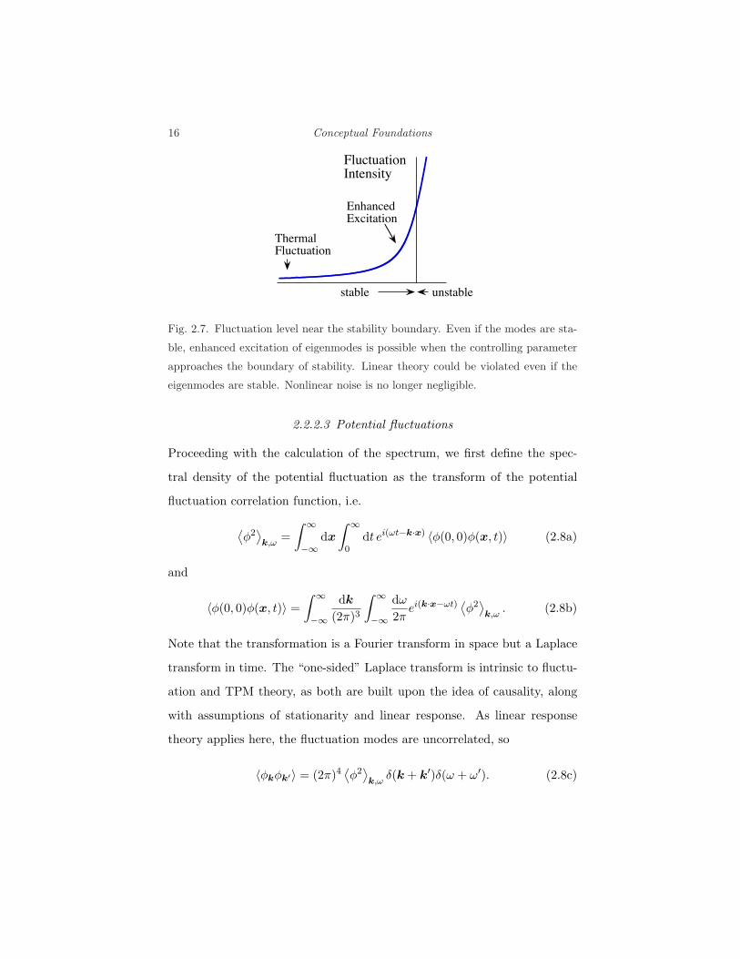
behavior of fluctuation levels near the stability boundary is schematically
illustrated in Fig.2.7. Even if the modes are stable, enhanced excitation of
eigenmodes is possible when the controlling parameter is sufficiently close to
the boundary of stability, approaching from below. Linear response theory
could be violated even if the eigenmodes are stable.
16 Conceptual Foundations
!"#$%#&%'()*)%+),'%
,%&."+ #),%&."+
/)0&)$+1/$'%&%'()
30+45&"!"#$%#&%'()
Fig. 2.7. Fluctuation level near the stability boundary. Even if the modes are sta-
ble, enhanced excitation of eigenmodes is possible when the controlling parameter
approaches the boundary of stability. Linear theory could be violated even if the
eigenmodes are stable. Nonlinear noise is no longer negligible.
2.2.2.3 Potential fluctuations
Proceeding with the calculation of the spectrum, we first define the spec-
tral density of the potential fluctuation as the transform of the potential
fluctuation correlation function, i.e.
⟨φ2
⟩k,ω
=∫ ∞
−∞dx
∫ ∞
0dt ei(ωt−k·x) 〈φ(0, 0)φ(x, t)〉 (2.8a)
and
〈φ(0, 0)φ(x, t)〉 =∫ ∞
−∞
dk
(2π)3
∫ ∞
−∞
dω
2πei(k·x−ωt)
⟨φ2
⟩k,ω
. (2.8b)
Note that the transformation is a Fourier transform in space but a Laplace
transform in time. The “one-sided” Laplace transform is intrinsic to fluctu-
ation and TPM theory, as both are built upon the idea of causality, along
with assumptions of stationarity and linear response. As linear response
theory applies here, the fluctuation modes are uncorrelated, so
〈φkφk′〉 = (2π)4⟨φ2
⟩k,ω
δ(k + k′)δ(ω + ω′). (2.8c)

2.2 Dressed Test Particle Model 17
Therefore, from Eqs.(2.8a)-(2.8c) and Eq.(2.6b), we can immediately pass
to the expression for the potential fluctuation spectrum,
⟨φ2
⟩k,ω
=(
4πn0
k2q
)2 ∫dv1
∫dv2
⟨f(1)f(2)
⟩
k,ω
|ε(k,ω)|2 . (2.9)
Note that the fluctuation spectrum is determined entirely by the discreteness
correlation function⟨f(1)f(2)
⟩and the dielectric function ε(k,ω). More-
over, we know ab-initio that since the plasma is in equilibrium at tem-
perature T , the fluctuation-dissipation theorem applies, so that the TPM
spectrum calculation must recover the general F-DT result, which is;⟨D2
⟩k,ω
4π=
2T
ωIm ε(k, ω). (2.10)
Here Dk,ω = ε(k, ω)Ek,ω is the electric displacement vector. Note that the
F-DT quite severely constrains the form of the particle discreteness noise.
2.2.2.4 Correlation of particles and fluctuation spectrum
To calculate⟨f(1)f(2)
⟩
k,ω, we must first determine
⟨f(1)f(2)
⟩. Since f is
the distribution of discrete uncorrelated test particles, we have;
f(x, v, t) =1n
N∑
i=1
δ(x− xi(t))δ(v − vi(t)). (2.11)
From Eqs. (2.3), (2.4), and (2.11), we obtain
⟨f(1)f(2)
⟩=
∫dxi
∫dvi
〈f〉n
N∑
i,j=1
[δ(x1 − xi(t))
× δ(x2 − xj(t))δ(v1 − vi(t))δ(v2 − vj(t))]. (2.12)
Since the product of δ’s is non-zero only if the arguments are interchangeable,
we obtain immediately the discreteness correlation function⟨f(1)f(2)
⟩=〈f〉n
δ(x1 − x2)δ(v1 − v2). (2.13)

18 Conceptual Foundations
Equation.(2.13) gives the discreteness correlation function in phase space.
Since the physical model is one of an ensemble of discrete, uncorrelated test
particles, it is no surprise that⟨f(1)f(2)
⟩is singular, and vanishes unless
the two points in phase space are coincident. Calculation of the fluctuation
spectrum requires the velocity integrated discreteness correlation function
C(k,ω) which, using spatial homogeneity, is given by:
C(k,ω) =∫
dv1
∫dv2
⟨f(1)f(2)
⟩
k,ω
=∫
dv1
∫dv2
[ ∫ ∞
0dτ eiωτ
∫dx e−ik·x
⟨f(0)f(x, τ)
⟩
+∫ 0
−∞dτ e−iωτ
∫dx e−ik·x
⟨f(x,−τ)f(0)
⟩]. (2.14)
Note that the time history which determines the frequency dependence of
C(k,ω) is extracted by propagating particle (2) forward in time and particle
(1) backward in time, resulting in the two Laplace transforms in the expres-
sion for C(k,ω). The expression for C(k,ω) can be further simplified by
replacing v1, v2 with (v1 ± v2)/2, performing the trivial v-integration, and
using unperturbed orbits to obtain
C(k,ω) = 2∫
dv
∫ ∞
0dτ eiωτ
∫dx e−ik·x 〈f(v)〉
nδ(x− vτ)
= 2∫
dv〈f(v)〉
n
∫ ∞
0dτ ei(ω−k·v)τ
=∫
dv 2π〈f(v)〉
nδ(ω − k · v). (2.15)
Equation (2.15) gives the well known result for the density fluctuation corre-
lation function in k,ω of an ensemble of discrete, uncorrelated test particles.
C(k,ω) is also the particle discreteness noise spectrum. Note that C(k,ω)
is composed of the unperturbed orbit propagator δ(ω − k · v), a weighting
function 〈f〉 giving the distribution of test particle velocities, and the factor
of 1/n, which is a generic measure of discreteness effects. Substitution of

2.2 Dressed Test Particle Model 19
C(k,ω) into Eq.(2.9) then finally yields the explicit general result for the
TPM potential fluctuation spectrum:
⟨φ2
⟩k,ω
=(
4πn0
k2q
)2 ∫dv 2π
n 〈f〉 δ(ω − k · v)|ε(k,ω)|2 . (2.16)
2.2.2.5 One-dimensional plasma
In order to elucidate the physics content of the fluctuation spectrum, it is
convenient to specialize the discussion to the case of a 1D plasma, for which:
C(k, ω) =2π
n|k|vTF (ω/k) (2.17a)
⟨φ2
⟩k,ω
= n0
(4πq
k2
)2 2π
|k|vT
F (ω/k)|ε(k,ω)|2 . (2.17b)
Here, F refers the average distribution function, with the normalization fac-
tor of vT extracted, 〈f (v)〉 = (n/vT )F (v), and vT is a thermal velocity. It
is interesting to observe that⟨φ2
⟩k,ω∼ (density) × (Coulomb spectrum) ×
(propagator) × (particle emission spectrum) × (screening). Thus, spectral
line structure in the TPM is determined by the distribution of Cerenkov
emission from the ensemble of discrete particles (set by 〈f〉) and the collec-
tive resonances (where ε(k,ω) becomes small).
In particular, for the case of an electron plasma with stationary ions, the
natural collective mode is the electron plasma wave, with frequency ω )
ωp(1 + γk2λ2D)1/2 (γ: specific heat ratio of electrons). So for ω # ωp, kvT ,
ε→ 1, we have;
⟨φ2
⟩k,ω) n0
(4πq
k2
)2 2π
|k|vTF (ω/k), (2.18a)
where F ∼ exp[−ω2/k2v2T ] for a Maxwellian distribution, while in the op-
posite limit of ω $ ωp, kvT where ε→ 1 + k−2λ−2D , the spectrum becomes
⟨φ2
⟩k,ω) n0(4πq)2
2π
|k|vT
(1 + 1/k2λ2
D
)−2. (2.18b)

20 Conceptual Foundations
In the first, super-celerity limit, the discrete test particle effectively decou-
ples from the collective response, while in the second, quasi-static limit, the
spectrum is that of an ensemble of Debye-screened test particles. This re-
gion also corresponds to the kλDe # 1 range, where the scales are too small
to support collective modes. In the case where collective modes are weakly
damped, one can simplify the structure of the screening response via the
pole approximation, which is obtained by expanding about ωk, i.e.
ε(k, ω) = εr(k,ω) + iIm ε(k,ω)
) εr(k,ωk) + (ω − ωk)∂ε
∂ω
∣∣∣∣ωk
+ iIm ε(k, ωk). (2.19)
So since εr(k, ωk) ≈ 0,
1/|ε|2 ) 1|Im ε|
|Im ε|
(ω − ωk)2| ∂ε∂ω |2 + |Im ε|2
) 1|Im ε| |∂εr/∂ω| · δ (ω − ωk) . (2.20)
Here it is understood that Im ε and ∂εr/∂ω are evaluated at ωk. Notice
that in the pole approximation, eigenmode spectral lines are weighted by
the dissipation Im ε.
The fluctuation spectrum of plasma oscillations in thermal equailibrium
is shown in Fig.2.8. The real frequency and the damping rate of the plasma
oscillation are shown as a function of the wavenumber in (a). In the regime
of kλDe $ 1, the real frequency is close to the plasma frequency, ω ∼ ωp, and
the damping rate is exponentially small. The power spectrum of fluctuation
as a function of the frequency is illustrated in (b) for various values of the
wave number. In the regime of kλDe $ 1, a sharp peak appears near the
eigenfrequency ω ∼ ωk. Owing to the very weak damping, the line width is
narrow. As the mode number becomes large (in the regime of kλDe ∼ 1), the
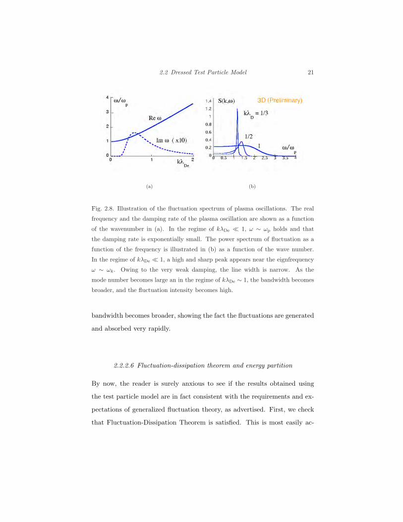
2.2 Dressed Test Particle Model 21
(a) (b)
Fig. 2.8. Illustration of the fluctuation spectrum of plasma oscillations. The real
frequency and the damping rate of the plasma oscillation are shown as a function
of the wavenumber in (a). In the regime of kλDe $ 1, ω ∼ ωp holds and that
the damping rate is exponentially small. The power spectrum of fluctuation as a
function of the frequency is illustrated in (b) as a function of the wave number.
In the regime of kλDe $ 1, a high and sharp peak appears near the eignfrequency
ω ∼ ωk. Owing to the very weak damping, the line width is narrow. As the
mode number becomes large an in the regime of kλDe ∼ 1, the bandwidth becomes
broader, and the fluctuation intensity becomes high.
bandwidth becomes broader, showing the fact the fluctuations are generated
and absorbed very rapidly.
2.2.2.6 Fluctuation-dissipation theorem and energy partition
By now, the reader is surely anxious to see if the results obtained using
the test particle model are in fact consistent with the requirements and ex-
pectations of generalized fluctuation theory, as advertised. First, we check
that Fluctuation-Dissipation Theorem is satisfied. This is most easily ac-

22 Conceptual Foundations
complished for the case of a Maxwellian plasma. There
Im ε = −ω2
pπ
k|k|∂ 〈f〉∂v
∣∣∣∣ω/k
=2πω
k2v2T
ω2p
|k|vTFM(
ω
k), (2.21a)
so using Eq.(2.21a) to relate Im ε(k, ω) to F (ω/kvT ) in Eq.(2.17b) gives
⟨φ2
⟩k,ω
=8πT
k2ω
Im ε
|ε|2 , (2.21b)
so we finally obtain ⟨D2
⟩k,ω
4π=
2T
ωIm ε (2.21c)
is in precise agreement with the statement of the F-DT for a classical, plasma
at temperature T . It is important to re-iterate here that applicability of
the F-DT rests upon to the applicability of linear response theory for the
emission and absorption of each mode. Both fail as the instability marginal
point is approached (from below).
Second, we also examine the k-spectrum of energy, with the aim of com-
paring the TPM prediction to standard expectations for thermal equilib-
rium, i.e. to see whether energy is distributed according to the conventional
wisdom of “T/2 per degree-of-freedom” . To this end, it is useful to write
(using Eq. (2.21)) the electric field energy as;
|Ek,ω|2
8π=
4πnq2
k|k|
F (ω/k)
(1− ω2p
ω2 )2 + (πω2p
k|k|F′)2
, (2.22)
where εr ) 1 − ω2p/ω2 for plasma waves, and F ′ = dF/du|ω/k. The total
electric field energy per mode Ek is given by
Ek =∫
dω |Ek,ω|2/8π, (2.23a)
so that use of the pole approximation to the collective resonance and a short
calculation then gives
Ek =neωp
2|k|F
|F ′| =T
2. (2.23b)

2.2 Dressed Test Particle Model 23
So, yes – the electric field energy for plasma waves is indeed equipartioned!
Since for plasma waves the particle kinetic energy density Ekin equals the
electric field energy density Ek (i.e. Ekin = Ek), the total wave energy
density per mode Wk is constant at T . Note that Eq. (2.23b) does not
imply the divergence of total energy density. Of course, some fluctuation
energy is present at very small scales (kλDe " 1) which cannot support
collective modes. On such scales, the pole expansion is not valid and simple
static screening is a better approximation. A short calculation gives, for
k2λ2De > 1, Ek
∼= (T/2)/k2λ2De , so that the total electric energy density is
⟨E2
8π
⟩=
∫dk Ek
=∫ ∞
−∞
dk
2π
T/2(1 + k2λ2
De)∼
(nT
2
)(1
nλDe
). (2.24)
As Eq. (2.24) is for 1D, there n has the dimensions of particles-per-distance.
In 3D, the analogue of this result is⟨
E2
8π
⟩∼
(nT
2
)(1
nλ3De
). (2.25)
so that the total electric field energy equals the total thermal energy times
the discreteness factor 1/nλ3De ∼ 1/N , where N is the number of particles in
a Debye sphere. Hence⟨E2/8π
⟩$ nT/2, as is required for a plasma with
weak correlations.
2.2.3 Relaxation Near Equilibrium and the Balescu-Lenard
Equation
Having determined the equilibrium fluctuation spectrum using the TPM,
we now turn to the question of how to use it to calculate relaxation near
equilibrium. By “relaxation” we mean the long time evolution of the mean
(i.e. ensemble averaged) distribution function 〈f〉. Here ‘long time’ means

24 Conceptual Foundations
long or slow evolution in comparison to fluctuation time scales. Generally,
we expect the mean field equation for the prototypical example of a 1D
electrostatic plasma to have the form of a continuity equation in velocity
space, i.e.
∂ 〈f〉∂t
= − ∂
∂vJ(v). (2.26)
Here, J(v) is a flux or current and 〈f〉 is the corresponding coarse grained
phase space density. J −−−−→v→±∞
0 assures conservation of total 〈f〉. The
essence of the problem at hand is how to actually calculate J(v)! Of course
it is clear from the Vlasov equation that J(v) is simply the average accel-
eration 〈(q/m)Eδf〉 due to the phase space density fluctuation δf . Not
surprisingly, then, J(v) is most directly calculated using a mean field ap-
proach. Specifically, simply substitute the total δf into 〈(q/m)Eδf〉 to cal-
culate the current J(v). Since δf = f c + f , J(v) will necessarily consist of
two pieces. The first piece, 〈(q/m)Ef c〉, accounts for the diffusion in veloc-
ity driven by the TPM potential fluctuation spectrum. This contribution
can be obtained from a Fokker-Planck calculation using the TPM spectrum
as the noise. The second piece,⟨(q/m)Ef
⟩, accounts for relaxation driven
by the dynamic friction between the ensemble of discrete test particles and
the Vlasov fluid. It accounts for the evolution of 〈f〉 which must accompany
the slowing down of a test particle by wave drag. The second piece has the
structure of a drag term. As is shown in the derivation of Eq. (2.16), 〈Ef c〉
ultimately arises from the discreteness of particles, f1.
The kinetic equation for 〈f〉 which results from this mean field calcula-
tion was first derived by R.Balescu and A. Lenard, and so is named in their
honor. The diffusion term of the Balescu-Lenard (B-L) equation is very
similar to the quasilinear diffusion operator, discussed in Chapter 3, though

2.2 Dressed Test Particle Model 25
the electric field fluctuation spectrum is prescribed by the TPM and the
frequency spectrum is not restricted to eigenmode frequency lines, as in the
quasilinear theory. The total phase space current J(v) is similar in structure
to that produced by the glancing, small angle Coulomb interactions which
the Landau collision integral calculates. However, in contrast to the Landau
theory, the B-L equation incorporates both static and dynamic screening,
and so treats the interaction of collective processes with binary encounters.
Screening also eliminates the divergences in the Landau collision integral (i.e.
the Coulomb logarithm) which are due to long range electrostatic interac-
tions. Like the Landau integral, the B-L equation is ultimately nonlinear in
〈f〉.
At this point, the skeptical reader will no doubt be entertaining question
like “What kind of relaxation is possible here?”, “How does it differ from
the usual collisional relaxation process?” and “Just what, precisely, does
‘near equilibrium’ mean?”. One point relevant to all these questions is that
it is easy to define states which have finite free energy, but which are stable
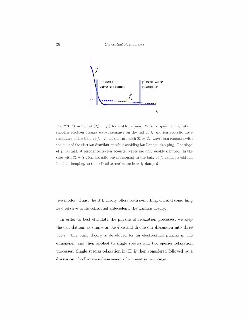
to collective modes. One example is the current driven ion acoustic (CDIA)
system shown in Fig.2.9. Here the non-zero current, which shifts the elec-
tron Maxwellian, constitutes free energy. However, since the shift does not
produce a slope in 〈fe〉 sufficient to overcome ion Landau damping, the free
energy is not accessible to linear CDIA instabilities. Nevertheless, electron
→ ion momentum transfer is possible, and can result in electron relaxation,
since the initial state is not one of maximum entropy. Here, relaxation oc-
curs via binary interactions of dressed test particles. Note however, that in
this case relaxation rates may be significantly faster than for ’bare’ particle
collisions, on account of fluctuation enhancement by weakly damped collec-
26 Conceptual Foundations
!!
!"# $%"&'(!%
)$+ ,+'"#$#%+
!+
-.$'/$ )$+
,+'"#$#%+
!
Fig. 2.9. Structure of 〈fi〉 , 〈fe〉 for stable plasma. Velocity space configuration,
showing electron plasma wave resonance on the tail of fe and ion acoustic wave
resonance in the bulk of fe, fi. In the case with Te # Ti, waves can resonate with
the bulk of the electron distribution while avoiding ion Landau damping. The slope
of fe is small at resonance, so ion acoustic waves are only weakly damped. In the
case with Te ∼ Ti, ion acoustic waves resonant in the bulk of fe cannot avoid ion
Landau damping, so the collective modes are heavily damped.
tive modes. Thus, the B-L theory offers both something old and something
new relative to its collisional antecedent, the Landau theory.
In order to best elucidate the physics of relaxation processes, we keep
the calculations as simple as possible and divide our discussion into three
parts. The basic theory is developed for an electrostatic plasma in one
dimension, and then applied to single species and two species relaxation
processes. Single species relaxation in 3D is then considered followed by a
discussion of collective enhancement of momentum exchange.
2.2 Dressed Test Particle Model 27
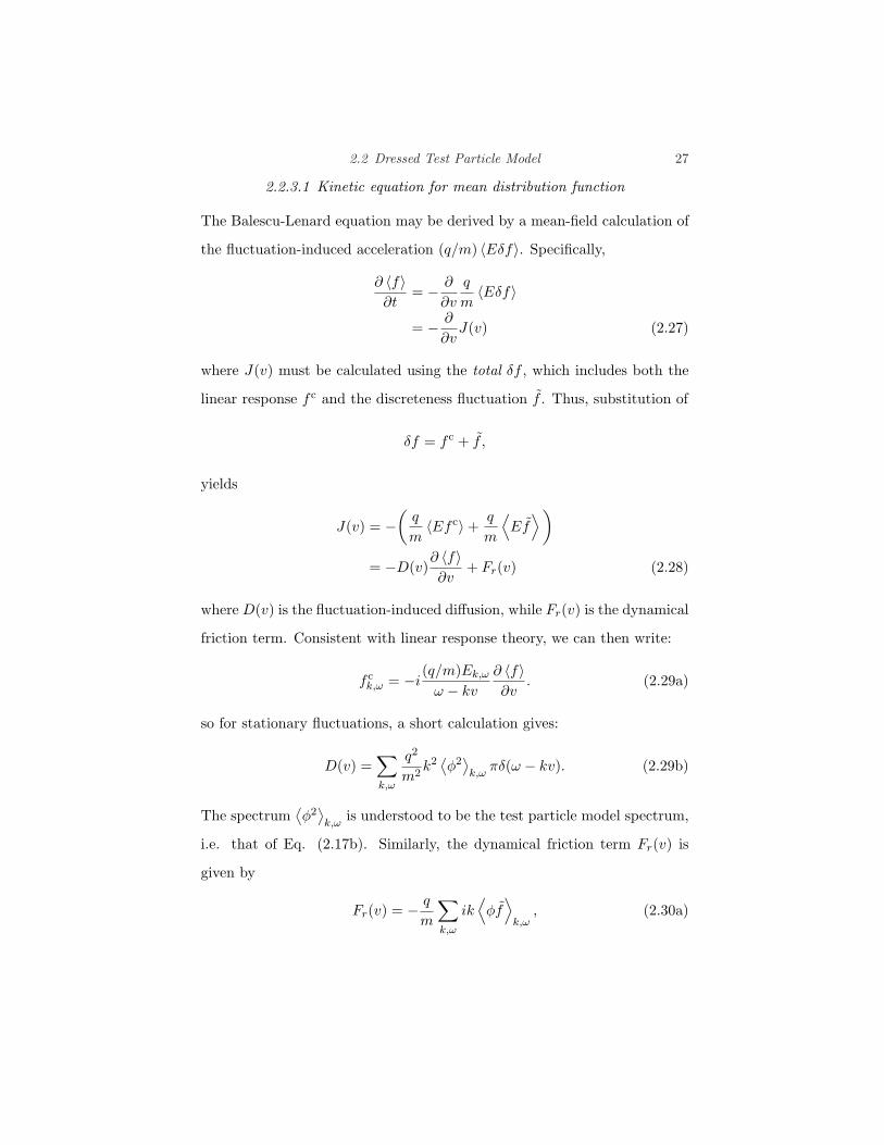
2.2.3.1 Kinetic equation for mean distribution function
The Balescu-Lenard equation may be derived by a mean-field calculation of
the fluctuation-induced acceleration (q/m) 〈Eδf〉. Specifically,
∂ 〈f〉∂t
= − ∂
∂v
q
m〈Eδf〉
= − ∂
∂vJ(v) (2.27)
where J(v) must be calculated using the total δf , which includes both the
linear response f c and the discreteness fluctuation f . Thus, substitution of
δf = f c + f ,
yields
J(v) = −(
q
m〈Ef c〉+ q
m
⟨Ef
⟩)
= −D(v)∂ 〈f〉∂v
+ Fr(v) (2.28)
where D(v) is the fluctuation-induced diffusion, while Fr(v) is the dynamical
friction term. Consistent with linear response theory, we can then write:
f ck,ω = −i
(q/m)Ek,ω
ω − kv
∂ 〈f〉∂v
. (2.29a)
so for stationary fluctuations, a short calculation gives:
D(v) =∑
k,ω
q2
m2k2
⟨φ2
⟩k,ω
πδ(ω − kv). (2.29b)
The spectrum⟨φ2
⟩k,ω
is understood to be the test particle model spectrum,
i.e. that of Eq. (2.17b). Similarly, the dynamical friction term Fr(v) is
given by
Fr(v) = − q
m
∑
k,ω
ik⟨φf
⟩
k,ω, (2.30a)

28 Conceptual Foundations
where, via Eq. (2.6b), we have:
⟨φf
⟩
k,ω=
4πn0q
k2
∫dv
⟨f f
⟩
k,ω
ε(k,ω)∗. (2.30b)
This result explains that the discreteness of particles are the source of cor-
relations in the excited mode. Since
⟨φ2
⟩k,ω
=(
4πn0q
k2
)2 C(k,ω)|ε(k,ω)|2
,
and ( from Eq. (2.14) )
C(k, ω) =⟨n2
⟩k,ω
=∫
dv 2πδ(ω − kv) 〈f(v)〉 ,
we have⟨φf
⟩
k,ω=
(4πn0q
k2
)2πδ(ω − kv) 〈f〉
n0|ε(k,ω)|2 .
Thus, the current J(v) is given by;
J(v) = −D(v)∂ 〈f〉∂v
+ Fr(v)
= −∑
k,ω
(4πn0q
k2
)q
m
(2πδ(ω − kv)n0|ε(k,ω)|2
)k
×(
4πn0q
k2
)πk
|k|vT
(q
m
)F (
ω
k)∂ 〈f〉∂v
+ Im ε(k,ω) 〈f〉
. (2.31)
Note that the contributions from the diffusion D(v) and dynamical friction
Fr(v) have been grouped together within the brackets. Poisson’s equation
relates ε(k, ω) to the electron and ion susceptibilities χ(k,ω) by
ε(k,ω) =(
1 +4πn0q
k2
)[χi(k,ω)− χe(k,ω)
],
where χi, χe are the ion and electron susceptibilities defined by
nk,ω = χi(k, ω)φk,ω.
It is straightforward to show that
Im ε(k, ω) = −πω2
p
k2
k
|k|vTF ′(ω/k) + Im εi(k, ω), (2.32a)

2.2 Dressed Test Particle Model 29
where
Im εi(k,ω) =4πn0q
k2Imχi(k,ω). (2.32b)
Here εi(k, ω) is the ion contribution to the dielectric function. Thus, we
finally obtain a simplified expression for J(v), which is
J(v) = −∑
k,ω
(ω2
p
k2
)2( 2π2
n0kvT
)δ(ω − kv)|ε(k, ω)|2
×
F(ω
k
) ∂ 〈f〉∂v
− 〈f(v)〉F ′(ω
k
)+ Im εi(k,ω) 〈f〉
. (2.33)
Equation (2.33) gives the general form of the velocity space electron cur-
rent in the B-L equation for electron relaxation, as described within the
framework of the TPM.
In order to elucidate the physics content of J(v), it is instructive to re-
write Eq. (2.33) in alternate forms. One way is to define the fluctuation
phase velocity by u = ω/k, so that
J(v) = −∑
k,ω
(ω2
p
k2
)2( 2π2
n0kvT
)δ(u− v)
|k||ε(k, ω)|2
×
F (u) 〈f(v)〉′ − F ′(u) 〈f(v)〉+ Im εi(k, ω) 〈f(v)〉
. (2.34)
Alternatively, one could just perform the summation over frequency to ob-
tain
J(v) = −∑
k
(ω2
p
k2
)2( π
n0kvT
)1
|ε(k, kv)|2
×
F (v)∂ 〈f(v)〉
∂v− 〈f(v)〉F ′(v) + Im εi(k, kv) 〈f(v)〉
. (2.35)
Finally, it is also useful to remind the reader of the counterpart of Eq.(2.33)
in the unscreened Landau collision theory, which we write for 3D as:
Jα(p) = −∑
e,i
∫
qα
d3q
∫d3p′W (p, p′, q)qαqβ
f(p′)
∂f(p)∂pβ
− ∂f(p′)∂p′β
f(p)
.
(2.36)

30 Conceptual Foundations
In Eq.(2.36), W (p,p′, q) is the transition probability for a collision (with
momentum transfer q) between a ‘test particle’ of momentum p and a ‘field
particle’ of momentum p′. Here the condition |q| $ |p|, |p|′ applies, since
long range Coulomb collisions are ‘glancing’.
2.2.3.2 Offset on Landau-Rosenbluth Theory
Several features of J(v) are readily apparent. First, just as in the case of the
Landau theory, the current J(v) can be written as a sum of electron-electron
and electron-ion scattering terms, i.e.
J(v) = −[De,e(v)
∂ 〈f〉∂v
+ Fe,e(v) + Fe,i(v)]. (2.37)
Here De,e(v) refers to the diffusion (in velocity) of electrons by fluctuations
excited by electron discreteness emission, Fe,e(v) is the dynamical friction
on electrons due to fluctuations generated by discreteness, while Fe,i is the
electron-ion friction produced by the coupling of emission (again due to
electron discreteness) to dissipative ion absorption. Interestingly, in 1D,
−De,e(v)∂ 〈f〉∂v
+ Fe,e(v) ∼ δ(u− v)−F (u) 〈f〉′ + F ′ 〈f〉 = 0,
since F = 〈f〉 for single species interaction. Thus, we see that electron -
electron friction exactly cancels electron diffusion in 1D. In this case,
J(v) ∼ δ(u− v)Im εi(k, ω) 〈fe(v)〉
so that electron relaxation is determined solely by electron-ion friction. This
result is easily understood from consideration of the analogy between same-
species interaction in a stable, 1D plasma and like-particle collisions in 1D
(Fig.2.10). On account of conservation of energy and momentum, it is trivial
to show that such collisions leave final state = initial state, so no entropy
production is possible and no relaxation can occur. This fact is manifested in

2.2 Dressed Test Particle Model 31
!"!#!$%
&!"$%
!"# !$#
Fig. 2.10. Like-Particle collisions in (a)1D and (b)3D.
the B-L theory by the cancellation between electron - electron terms - since
the only way to produce finite momentum transfer in 1D is via inter-species
collisions, the only term which survives in J(v) is Fe,i(v). Note that this
result is not a purely academic consideration, since a strong magnetic field
B0 often imposes a 1D structure on the wave -particle resonance interaction
in more complicated problems.
A detail comparison and contrast between the Landau theory of collisions
and the B-L theory of near-equilibrium relaxation is presented in Table 2.2.
2.2.3.3 Resistivity (Relaxation in one-dimensional system)
Having derived the expression for J(v), it can then be used to calculate
transport coefficients and to macroscopically characterize relaxation. As an
example, we consider the effective resistivity associated with the current
driven system of Fig.2.9. To constract an effective Ohm’s Law for this

32 Conceptual Foundations
Table 2.2. Comparison of Landau and Balescu-Lenard relaxation theory
Laudau Theory B-L Theory
Physical
scenario
‘test’ particle
scattered by distribution
of ‘field’ particles
test particle scattered by
distribution of fluctuations
with vph = ω/k,
produced via discreteness
Scatterer
distribution
f(p′)
field particles distribution
F (u), u = ω/k
fluctuation phase velocity
distribution
Correlation
uncorrelated particles as discrete uncorrelated
assumed molecular chaos, test particles,
〈f(1, 2)〉 = 〈f(1)〉 〈f(2)〉⟨f f
⟩= (〈f〉 /n)δ(x )δ(v )
Screening
none -
1/|ε(k,ω)|2Coulomb lnΛ factor
put in ‘by intuition’
Scattering
strength
|q|$ |p| linear response and
weak deflection unperturbed orbits
Interaction
Selection Rule
W (p,p′, q) = δ(p− p′) δ(u− v) in 1D
in 1D, 1 species δ(k · (v − v′)) in 3D
system, we simply write
∂ 〈f〉∂t
+q
mE0
∂ 〈f〉∂v
= −∂J(v)∂v
, (2.38a)
and then multiply by n0qv and integrate to obtain, in the stationary limit,
E0 = −4πn0q
ω2p
∫dv J(v)
= 4πn0|q|∑
k,ω
ω2p
(k2)2(2π/|k|)n0kvT
(Im εi(k, ω)|ε(k, ω)|2
) ⟨fe
(ω
k
)⟩
≡ ηeffJ0. (2.38b)
Not surprisingly, the response of 〈fe〉 to E0 cannot unambiguously be written
as a simple, constant effective resistivity, since the resonance factor δ(ω −

2.2 Dressed Test Particle Model 33
kv) and the k, ω dependence of the TPM fluctuation spectrum conflate the
field particle distribution function with the spectral structure. However, the
necessary dependence of the effective resistivity on electron-ion interaction
is readily apparent from the factor of Im εi(k, ω). In practice, a non-trivial
effect here requires a finite but not excessively strong overlap of electron and
ion distributions. Note also that collective enhancement of relaxation below
the linear instability threshold is possible, should Im ε(k, ω) become small.
2.2.3.4 Relaxation in three-dimensional system
Having discussed the 1D case at some length, we now turn to relaxation
in 3D. The principal effect of three dimensionality is to relax the tight link
between particle velocity v and fluctuation phase velocity (ω/|k|)k. Alter-
natively put, conservation constraints on like-particle collisions in 1D force
the final state = initial state, but in 3D, glancing collisions which conserve
energy and the magnitude of momentum |p|, but change the particle’s di-
rections, are possible. The contrast between 1D and 3D is illustrated in
Fig.2.10. In 3D, the discreteness correlation function is
C(k, ω) = 〈nn〉k,ω =∫
d3 v2π
n0δ(ω − k · v) 〈f〉 . (2.39)
So the B-L current J(v) for like particle interactions becomes:
J(v) = −∑
k,ω
(ω2
p
k2
)2 2π2δ(ω − k · v)vT n0|ε(k, ω)|2
× k
∫dv′ δ(ω − k · v′)
⟨f(v′)
⟩k · ∂ 〈f〉
∂v
−∫
dv′ δ(ω − k · v′)k · ∂ 〈f〉∂v′
〈f(v)〉
. (2.40a)
Note that the product of delta functions can be re-written as
δ(ω − k · v)δ(ω − k · v′) = δ(ω − k · v)δ(k · v − k · v′).
34 Conceptual Foundations
We thus obtain an alternate form for J(v), which is
J(v) = −∑
k,ω
(ω2
p
k2
)2 2π2δ(ω − k · v)vT n0|ε(k, ω)|2
×
k
∫dv′ δ(k · v − k · v′)
[ ⟨f(v′)
⟩k · ∂ 〈f〉
∂v− k · ∂ 〈f〉
∂v′〈f(v)〉
].
(2.40b)
This form illustrates an essential aspect of 3D, which is that only the parallel
(to k) components of test and field particle velocities v and v′ need be equal
for interaction to occur. This is in distinct contrast to the case of 1D, where
identity, i.e. v = v′ = u, is required for interaction. Thus, relaxation by
like-particle interaction is possible, and calculations of transport coefficients
are possible, following the usual procedures of the Landau theory.
2.2.3.5 Dynamic Screening
We now come to our final topic in B-L theory, which is dynamic screening. It
is instructive and enlightening to develop this topic from a direction slightly
different than that taken by our discussion up till now. In particular, we
will proceed from the Landau theory, but will calculate momentum transfer
including screening effects and thereby arrive at a B-L equation.
2.2.3.6 Relaxation in Landau model
Starting from Eq. (2.36), the Landau theory expression for the collision-
induced current (in velocity) may be written as
Jα(p) =∑
species
∫d3p′
[f(p)
∂f(p′)∂p′β
− f(p′)∂f(p)∂pβ
]Bα,β , (2.41a)
where
Bα,β =12
∫dσ qαqβ|v − v′|. (2.41b)

2.2 Dressed Test Particle Model 35
The notation here is standard: dσ is the differential cross section and q
is the momentum transfer in the collision. We will calculate Bα,β directly,
using the some physics assumptions as in the TPM. A background or ‘field’
particle with velocity v′, and charge e′ produces a potential field
φk,ω =4πe′
k2ε(k, ω)2πδ(ω − k · v′), (2.42a)
so converting the time transform gives
φk(t) =4πe′
k2ε(k,k · v′)e−ik·v′t. (2.42b)
From this, it is straightforward to calculate the net deflection or momentum
transfer q by calculating the impulse delivered to a test particle with charge
e moving along an unperturbed trajectory of velocity v. This impulse is:
q = −∫
r=+vt
∂V
∂rdt, (2.43a)
where the potential energy V is just
V = eφ
= 4πee′∫
d3keik·re−ik·v′t
k2ε(k, k · v′) . (2.43b)
Here ρ is the impact parameter for the collision, a cartoon of which is
sketched in Fig. 2.11. A short calculation then gives the net momentum
transfer q,
q = 4πee′∫
d3k
(2π3)−ikeik· 2πδ(k · (v − v′))
k2ε(k, k · v′)
= 4πee′∫
d2k⊥(2π3)
−ik⊥eik⊥·
k2ε(k, k · v′)|v − v′| . (2.44)
To obtain Eq. (2.44), we used
δ(k · (v − v′)) =δ(k‖)|v − v′| ,

36 Conceptual Foundations
!
!"#$%&'%($)
*%(+&
Fig. 2.11. Deflection orbit and unperturbed orbit
and the directions ‖ and ⊥ are defined relative to the direction of v − v′
Since J ∼ ρ2, we may write Bα,β as
Bα,β =∫
d2ρ qαqβ|v − v′|. (2.45)
Noting that the d2ρ integration just produces a factor of (2π)2δ(k⊥ + k′⊥),
we can then immediately perform one of the∫
d2k⊥ integrals in Bα,β to get
Bα,β = 2e2e′2∫
d2k⊥k⊥αk⊥β
|k2⊥ε(k, k · v′)|2|v − v′|
. (2.46)
It is easy to see that Eq.(2.46) for Bα,β (along with Eq.(2.41a)) is entirely
equivalent to the B-L theory for J(v). In particular, note the presence of
the dynamic screening factor ε(k, k ·v′). If screening is neglected, ε→ 1 and
Bα,β ∼∫
d2k⊥k2⊥
|ε|k4⊥∼
∫dk⊥/k⊥ ∼ ln(k⊥max/k⊥min)
which is the familiar Coulomb logarithmfrom the Landau theory. Note that

2.2 Dressed Test Particle Model 37
if k, ω → 0,
k2⊥ε ∼ k2
⊥ + 1/λ2D
so that Debye screening eliminates the long range, divergence (associated
with k⊥min) without the need for an ad-hoc factor. To make the final step
toward recovering the explicit B-L result, one can ‘un-do’ the dk‖ integration
and the frequency integration to find
Bα,β = 2(ee′)2∫ ∞
−∞dω
∫
k<kmax
d3k δ(ω−k·v)δ(ω−k·v′)kαkβ
k4|ε(k,ω)|2 . (2.47)
Here kmax is set by the distance of closest approach, i.e.
kmax ∼µv2
rel
2ee′.
Substituting Eq.(2.47) for Bα,β into Eq.(2.41a) recovers Eq.(2.40a). This
short digression convincingly demonstrates the equivalence of the B-L theory
to the Landau theory with dynamic screening.
2.2.3.7 Collective mode
We now explore the enhancement of relaxation by weakly damped collective
modes. Consider a stable, two species plasma with electron and ion distri-
bution functions as shown in Fig. 2.9. This plasma has no free energy (i.e.
no net current), but is not necessarily a maximum entropy state, if Te /= Ti.
Moreover, the plasma supports two types of collective modes, namely
i.) electron plasma waves, with vTe < ω/k.
ii.) ion acoustic waves, with vTi < ω/k < vTe,
where vTe and vTi are the electron and ion thermal speeds, respectively.
Electron plasma waves are resonant on the tail of 〈fe〉, where there are
few particles. Hence plasma waves are unlikely to influence relaxation in
a significant way. On the other hand, ion acoustic waves are resonant in

38 Conceptual Foundations
the bulk of the elctron distribution. Moreover, if Te # Ti, it is easy to
identify a band of electron velocities with significant population levels f but
for which ion Landau damping is negligible. Waves resonant there will be
weakly damped, and so may substantially enhance relaxation of 〈fe(v)〉. It is
this phenomenon of collectively enhanced relaxation that we seek to explore
quantitatively.
To explore collective enhancement of relaxation, we process from Eq.(2.47),
make a pole expansion around the ion acoustic wave resonance and note for
ion acoustic wave, ω < k · v (for electrons), so
Bα,β = 2πq4∫ ∞
−∞dω
∫d3k δ(k · v)δ(k · v′) δεr(k,ωk)
|Im ε(k,ω)| . (2.48)
Here εr(k,ωk) = 0 for wave resonance, and e = e′ = q, as scattered and field
particles are all electrons. Im ε(k,ω) refers to the collective mode dissipation
rate. Now, changing variables according to
R = k · n,
k1 = k · v, k2 = k · v′
n = v × v′/|v × v′|.
We have
d3k = dRdk1dk2/|v × v′|
so the k1, k2 integrals in Eq.(2.48) may be immediately performed, leaving
Bα,β =2πq4nαnβ
|v × v′| 2∫
R>0dk
∫ ∞
−∞dω
δ(εr(k,ω))R2|Im ε| . (2.49)
We remind the reader that this is the piece of Bα,β associated with field
particle speeds or fluctuation phase speeds v′ ∼ ω/k $ vTe for which the
collective enhancement is negligible and total J(v) is, of course, the sum of
both these contributions. Now, the dielectric function for ion acoustic waves

2.2 Dressed Test Particle Model 39
is
Re ε(k,ω) = 1−ω2
pi
ω2+
1k2λ2
D
. (2.50a)
Im ε(k,ω) =√
π
2ω
k3
(1
λ2DevTe
+1
λ2DivTi
e−ω2/2k2v2Ti
). (2.50b)
Here λDe and λDi are the electron and ion Debye lengths, respectively. An-
ticipating the result that
ω2 =k2c2
s
1 + k2λ2De
for ion acoustic waves, Eq.(2.50a, 2.50b) togother suggest that the strongest
collective enhancement will come from short wavelength (i.e. k2λ2De # 1),
because Im ε(k, ω) is smaller for these scales, since
Im ε(k, ω) ∼ 1k2λ2
De
ω
kvTe.
For such short wavelengths, then
δ(εr) ∼= δ(1− ω2pi/ω2)
=12ωpi
[δ(ω − ωpi) + δ(ω + ωpi)
].
Evaluating Bα,β, as given by Eqs. (2.48) and (2.49), in this limit then finally
gives,
Bα,β =(
4πq2ωpinαnβ
|v × v′|
) ∫dk
k2|Im ε(k, ωpi)|
=2√
2πq4vTeλ2De
|v × v′|λ2Di
nαnβ
∫dξ
/[1 + exp
(− 1
2ξ+
L
2
)], (2.51a)
where:
L = ln[(
Te
Ti
)2 mi
me
](2.51b)
and ξ = k2λ2De. Equation (2.51a) quite clearly illustrates that maximal
relaxation occurs for minimal Im ε(ξ, L), that is when exp[−1/2ξ + L/2] $
40 Conceptual Foundations
1. That is, the collective enhancement of discreteness-induced scattering is
determined by Im ε for the least damped mode. This occurs when ξ ! 1/L,
so that the dominant contribution to Bα,β comes from scales for which
k2 = (k · n)2 < 1/(λ2DeL).
Note that depending on the values of L and the Coulomb logarithm (ln Λ,
which appears in the standard Coulombic scattering contribution to Bα,β
from v′ ∼ vTe), the collectively enhanced Bα,β due to low velocity field
particles (v′ $ vTe) may even exceed its familiar Coulomb scattering coun-
terpart. Clearly, this is possible only when Te/Ti # 1, yet not so large as to
violate the tenets of the TPM and B-L theories.
2.2.4 Test Particle Model: Looking Back and Looking Ahead
In this section of the introductory chapter, we have presented the test par-
ticle model for fluctuations and transport near thermal equilibrium. As
we mentioned at the beginning of the chapter, the TPM is the most basic
and most successful fluctuation theory for weakly collisional plasmas. So,
despite its limitation to stable, quiescent plasmas, the TPM has served as
a basic paradigm for treatments of the far more difficult problems of non-
equilibrium plasma kinetics, such as plasma turbulence, turbulent transport,
self-organization etc. Given this state of affairs, we deem it instructive to
review the essential elements of the TPM and place the subsequent chap-
ters of this book in the context of the TPM and its elements. In this way,
we hope to provide the reader with a framework from which to approach
the complex and sometimes bewildering subject of the physical kinetics of
non-equilibrium plasmas. The discussion which follows is summarized in
Table 2.3. We discuss and compare the test particle model to its non-

2.2 Dressed Test Particle Model 41
equilibrium descendents in terms of both physics concepts and theoretical
constructs.
Regarding physics concepts, the TPM is fundamentally a “near equilib-
rium” theory, which presumes a balance of emission and absorption at each
k. In a turbulent plasma, non-linear interaction produces spectral transfer
and a spectral cascade, which de-localize the location of absorption from the
region of emission in k,ω space. A spectral transfer turbulence energy from
one region (i.e. emission) to another (i.e. damping). There two cases are
contrasted in Fig.2.1.
A second key concept in the TPM is that emission occurs only via Cerenkov
radiation from discrete test particles. Thus, since the only source for collec-
tive modes is discreteness, we always have
∇ · εE = 4πqδ(x− x(t))
so
⟨φ2
⟩k,ω
=⟨n2
⟩
|ε(k,ω)|2 .
In contrast, for non-equilibrium plasmas, nonlinear coupling produces inco-
herent emission so the energy in mode k evolves according to
∂
∂t
⟨E2
⟩k
+
(∑
k′
C(k, k′)⟨E2
⟩k′Tck,k′
)⟨E2
⟩k
+ γdk⟨E2
⟩k
=∑
p,qp+q=k
C(p, q)τc p,q⟨E2
⟩p
⟨E2
⟩q
+ SDk⟨E2
⟩k
(2.52)
where SDk is the discreteness source and γdk is the linear damping for the
mode k. For sufficient fluctuation levels, the nonlinear noise term (i.e. the
first on the RHS) will clearly dominate over discreteness. A similar comment
can be made in the context of the LHS of Eq.(2.52), written above. Nonlinear

42 Conceptual Foundations
Table 2.3. Test particle model and its non-equilibrium descendents:
physical concepts and theoretical constructs
Test Particle Model Non-Equilibrium Descendent
Physics Concepts
emission vs. absorption
balance per k
spectral cascade, transfer,
inertial range (Chapter 5, 6)
discreteness noiseincoherent mode-coupling (Chapter 5, 6),
granulation emission (Chapter 8)
relaxation by
screened collisions
collective instability driven relaxation,
quasilinear theory, granulation interaction
(Chapter 3, 8)
Theoretical Constructs
linear response
unperturbed orbit
turbulence response, turbulent diffusion,
resonance broadening (Chapter 4,6)
damped mode response
nonlinear dielectric,
wave-wave interaction,
wave kinetics (Chapter 5, 6)
mean field theorymean field theory without and with
granulations (Chapter 3, 8)
discreteness-driven
stationary spectrum
wave kinetics,
renormalized mode coupling,
disparate scale interaction (Chapter 5 - 7)
Balescu-Lenard,
screened Landau equations
quasilinear theory
granulation relaxation theory
(Chapter 3, 8)
damping will similarly eclipse linear response damping for sufficiently large
fluctuation levels.
A third physics concept is concerned with the mechanism physics of relax-
ation and transport. In the TPM, these occur only via screened collisions.
2.2 Dressed Test Particle Model 43
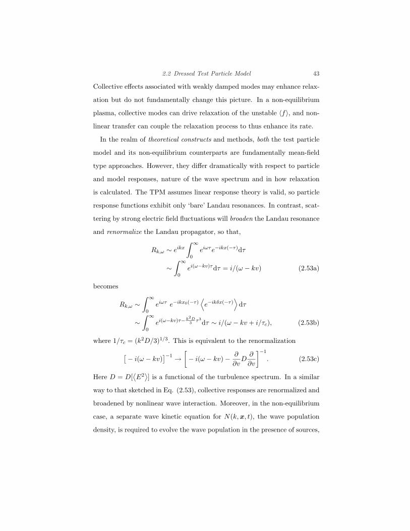
Collective effects associated with weakly damped modes may enhance relax-
ation but do not fundamentally change this picture. In a non-equilibrium
plasma, collective modes can drive relaxation of the unstable 〈f〉, and non-
linear transfer can couple the relaxation process to thus enhance its rate.
In the realm of theoretical constructs and methods, both the test particle
model and its non-equilibrium counterparts are fundamentally mean-field
type approaches. However, they differ dramatically with respect to particle
and model responses, nature of the wave spectrum and in how relaxation
is calculated. The TPM assumes linear response theory is valid, so particle
response functions exhibit only ‘bare’ Landau resonances. In contrast, scat-
tering by strong electric field fluctuations will broaden the Landau resonance
and renormalize the Landau propagator, so that,
Rk,ω ∼ eikx∫ ∞
0eiωτe−ikx(−τ)dτ
∼∫ ∞
0ei(ω−kv)τdτ = i/(ω − kv) (2.53a)
becomes
Rk,ω ∼∫ ∞
0eiωτ e−ikx0(−τ)
⟨e−ikδx(−τ)
⟩dτ
∼∫ ∞
0ei(ω−kv)τ− k2D
3 τ3dτ ∼ i/(ω − kv + i/τc), (2.53b)
where 1/τc = (k2D/3)1/3. This is equivalent to the renormalization
[− i(ω − kv)
]−1 →[− i(ω − kv)− ∂
∂vD
∂
∂v
]−1
. (2.53c)
Here D = D[⟨E2
⟩] is a functional of the turbulence spectrum. In a similar
way to that sketched in Eq. (2.53), collective responses are renormalized and
broadened by nonlinear wave interaction. Moreover, in the non-equilibrium
case, a separate wave kinetic equation for N(k,x, t), the wave population
density, is required to evolve the wave population in the presence of sources,
44 Conceptual Foundations
non-linear interaction and refraction, etc. by disparate scales. This wave
kinetic equation is usually written in the form
∂N
∂t+ (vg + v) ·∇N − ∂
∂x(ω + k · v) · ∂N
∂k= SkN + CK(N). (2.54)
Since in practical problems, the mean field or coarse grained wave popu-
lation density 〈N〉 is of primary interest, a similar arsenal of quasi-linear
type closure techniques has been developed for the purpose of extracting
〈N〉 from the wave kinetic equation. We conclude by noting that this dis-
cussion, which began with the TPM, comes full circle when one considers
the effect of nonlinear mode coupling on processes of relaxation and trans-
port. In particular, mode localized coupling produces phase space density
vortexes or eddys in the phase space fluid. These phase space eddys are
called granulations, and resemble a macroparticle. Such granulations are
associated with peaks in the phase space density correlation function. Since
these granulations resemble macroparticles, it should not be too surprising
that they drive relaxation via a mechanism similar to that of dressed test
particles. Hence, the mean field equation for 〈f〉 in the presence of granu-
lations has the structure of a Balescu-Lenard equation, though of course its
components differ from those discussed in this chapter.
2.3 K41 Beyond Dimensional Analysis - Revisiting the Theory of
Hydrodynamic Turbulence
We now turn to our second paradigm, namely Navier-Stokes turbulence,
and the famous Kolmogorov cascade through the inertial range. This is
the classic example of a system with dynamics controlled by a self-similar
spectral flux. It constitutes the ideal complement to the TPM, in that it
features the role of transfer, rather than emission and absorption. We also

2.3 K41 Beyond Dimensional Analysis 45
discuss related issues in particle dispersion, two-dimensional turbulence and
turbulent pipe flows.
2.3.1 Key Elements in Kolmogorov Theory of Cascade
2.3.1.1 Kolmogorov theory
Surely everyone has encountered the basic ideas of Kolmogorov’s theory
of high Reynolds number turbulence! Loosely put, empirically motivated
assumptions of
i) spatial homogeneity - i.e. the turbulence is uniformly distributed in
space,
ii) isotropy - i.e. the turbulence exhibits no preferred spatial orientation,
iii) self-similarity - i.e. all inertial range scales exhibit the same physics
and are equivalent. Here ”inertial range” refers to the range of scales 0
smaller than the stirring scale 00 but larger than the dissipation scale
(0d < 0 < 00),
iv) locality of interaction - i.e. the (dominant) nonlinear interactions in
the inertial range are local in scale, i.e. while large scales advect small
scales, they cannot distort or destroy small scales, only sweep them
around. Inertial range transfer occurs via like-scale straining, only.
Assumptions i) - iv) and the basic idea of an inertial range cascade are
summarized in Fig.2.12. Using assumptions i) - iv), we can state that energy
thru-put must be constant for all inertial range scales, so
ε ∼ v30/00 ∼ v(0)3/0, (2.55a)
and
v(0) ∼ (ε0)1/3, (2.55b)
46 Conceptual Foundations
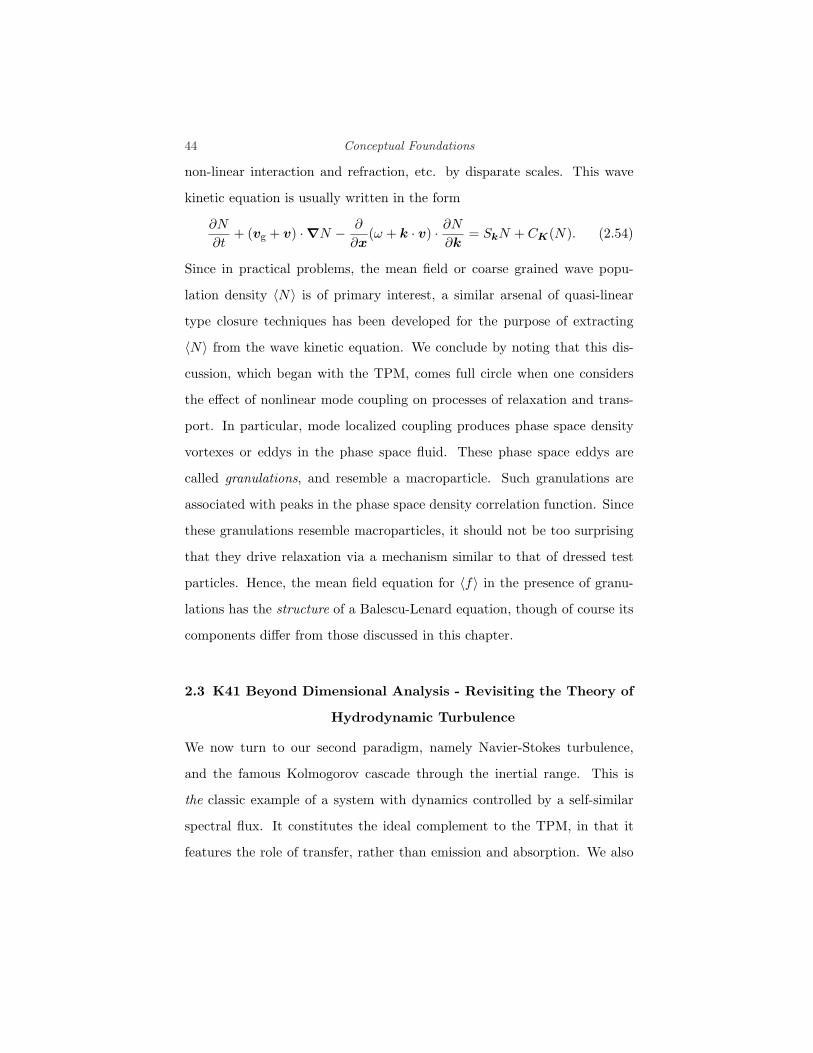
(a)
!"#$%&'()*+)*',&
-./0()/'1#2*."%
3"#$*.24'$2"%#
!"#$%&'."+)*
,&'/*.$$."% !"#$%'(')*+)$(-.')
/(0'/(')/$%)$(*'
(b)
. . . . . . . . . . . . . . . . . .
l0
ld
l1 = l0
ln = n l0
..........
..........
..........
..........
Fig. 2.12. Basic cartoon explanation of the Richardson-Kolmogorov cascade. En-
ergy transfer in Fourier-space (a), and real space (b).
E(k) ∼ ε2/3k−5/3, (2.55c)
which are the familiar K41 results. The dissipation scale 0d is obtained by
balancing the eddy straining rate ε1/3/02/3 with the viscous dissipation rate
ν/02 to find the Kolmogorov microscale,
0d ∼ ν3/4/ε1/4. (2.56)

2.3 K41 Beyond Dimensional Analysis 47
2.3.1.2 Richardson theory of particle separation
A related and important phenomenon, which also may be illuminated by
scaling arguments, is how the distance between two test particles grows in
time in a turbulent flow. This problem was first considered by Louis Fry
Richardson, who was stimulated by observations of the rate at which pairs
of weather balloons drifted apart from one another in the (turbulent) atmo-
sphere. Consistent with the assumption of locality of interaction in scale,
Richardson ansatzed that the distance between two points in a turbulent
flow increases at the speed set by the eddy velocity on scales correspond-
ing (and comparable) to the distance of separation (Fig. 2.13). Thus, for
distance 0,
d0
dt= v(0), (2.57a)
so using the K41 results (2.55b) gives
0(t) ∼ ε1/3t3/2, (2.57b)
a result which Richardson found to be in good agreement with observa-
tions. Notice that the distance of separation grows super-diffusively, i.e.
0(t) ∼ t3/2, and not ∼ t1/2, as in the textbook case of Brownian motion.
The super-diffusive character of 0(t) is due to the fact that larger eddys
support larger speeds, so the separation process is self-accelerating. Note
too, that the separation grows as a power of time, and not exponentially, as
in the case of a dynamical system with positive Lyapunov exponent. This
is because for each separation scale 0, there is a unique corresponding sepa-
ration velocity v(0), so in fact there is a continuum of Lyapunov exponents
(one for each scale) in the case of a turbulent flow. Thus, 0(t) is algebraic,
not exponential! By way of contrast, the exponential rate of particle pair

48 Conceptual Foundations
(a)
t
t' l
v (l)
(b)
v
lt
t'
(c)
t
t'
Fig. 2.13. Basic idea of the Richardson dispersion problem. The evolution of the
separation of the two points (black and white dots) l follows the relation dl/dt = v
(a). If the advection field scale exceeds l, the particle pair swept together, so l is
unchanged (b). If the advection field scale is less than l, there is no effect (except
diffusion) on particle dispersion (c).
separation in a smooth chaotic flow is set by the largest positive Lyapunov
exponent. We also remark here that while intermittency corrections to the
K41 theory based upon the notion of a dissipative attractor with a fractal
dimension less than three have been extensively discussed in the literature,
the effects of intermittency in the corresponding Richardson problem have
received relatively little attention. This is unfortunate, since, though it may

2.3 K41 Beyond Dimensional Analysis 49
seem heretical to say so, the Richardson problem is, in many ways, more
fundamental than the Kolmogorov problem, since unphysical effects due
to sweeping by large scales are eliminated by definition in the Richardson
problem. Moreover, the Richardson problem is of interest to calculating the
rate of turbulent dispersion and the lifetime of particles or quasiparticles
of turbulent fluid. An exception to the lack of advanced discussion of the
Richardson problem is the excellent review article by Falkovich, Gawedski
and Vergassola, 2001.
2.3.1.3 Stretching and generation of enstrophy
Of course, ‘truth in advertising’ compels us to emphasize that the scaling
arguments presented here contain no more physics than that which was in-
serted ab initio. To understand the physical mechanism underpinning the
Kolmogorov energy cascade, one must consider the dynamics of structures
in the flow. As is well known, the key mechanism in 3D Navier-Stokes tur-
bulence is vortex tube stretching, schematically shown in Fig. 2.14. There,
we see that alignment of strain ∇v with vorticity ω (i.e. ω ·∇v /= 0) gener-
ates small scale vorticity, as dictated by angular momentum conservation in
incompressible flows. The enstrophy (mean squared vorticity) thus diverges
as
〈ω2〉 ∼ ε/ν, (2.58)
for ν → 0. This indicates that enstrophy is produced in 3D turbulence, and
suggests that there may be a finite time singularity in the system, an issue
to which we shall return later. By finite time singularity of enstrophy, we
mean that the enstrophy diverges within a finite time (i.e. with a growth rate
which is faster than exponential). In a related vein, we note that finiteness
of ε as ν → 0 constitutes what is called an anomaly in quantum field theory.

50 Conceptual Foundations
!
!
!"$%&'%$()*+,
!-
!-
". / !. !..
!.
!.
"- / !- !-.
Fig. 2.14. The mechanism of enstrophy generation by vortex tube stretching. The
vortex tube stretching vigorously produces small scale vorticity.
An anomaly occurs when symmetry breaking (in this case, breaking of time
reversal symmetry by viscous dissipation) persists as the symmetry breaking
term in the field equation asymptotes to zero. The scaling 〈ω2〉 ∼ 1/ν is
suggestive of an anomaly. So is the familiar simple argument using the Euler
vorticity equation (for ν → 0 )
dω
dt= ω ·∇v, (2.59a)
d
dtω2 ∼ ω3. (2.59b)
2.3 K41 Beyond Dimensional Analysis 51
Of course, this “simple argument” is grossly over-simplified, and incorrect.†
In two dimensions ω · ∇v = 0, so enstrophy is conserved. As first shown
by Kraichnan, this necessitates a dual cascade, in which enstrophy forward
cascades to small scales, while energy inverse cascades to large scales. The
mechanism by which the dual conservation of energy and enstrophy force a
dual cascade in 2D turbulence is discussed further later in this chapter.
2.3.1.4 Fundamental hypothesis for K41 theory
As elegantly and concisely discussed by U. Frisch in his superb monograph
“Turbulence - The Legacy of A.N. Kolmogorov”, the K41 theory can be
systematically developed from a few fundamental hypotheses or postulates.
Upon proceeding, the cynical reader will no doubt conclude that the hy-
potheses H1)-H4) stated below are simply restatements of assumptions i)-
iv). While it is difficult to refute such a statement, we remark here that
H1)-H4), are indeed of value, both for their precise presentation of Kol-
mogorov’s deep understanding and for the insights into his thinking which
they provide. As these postulates involve concepts of great relevance to
other applications, we revisit them here in preparation for our subsequent
discussions. The first fundamental hypotheses of the K41 theory is:
H1) As Reynolds number Re → ∞, all possible symmetries of the Navier-
Stokes equation, usually broken by the means of turbulence initiation or
production, are restored in a statistical sense at small scales, and away from
boundaries.
† In fact, a mathematical proof of finite time singularity of enstrophy remains an elusive goal,
with an as-yet-unclaimed Clay prize of $1,000,000. (2007)
52 Conceptual Foundations
The reader should note that H1) is a deceptively simple, and fundamentally
quite profound hypothesis! The onset or production of turbulence nearly
always involves symmetry breaking. Some examples are:
i) shear flow turbulence: the initial Kelvin-Helmholtz instability results
from breaking of translation and rotation symmetry.
ii) turbulence in a pipe with a rough boundary: the driving pressure drop,
the wall and roughenings break symmetry.
iii) turbulence in a flushing toilet: the flow has finite chirality and is non-
stationary.
Naively, one might expect the turbulent state to have some memory of this
broken symmetry. Indeed, the essence of β-model and multi-fractal theories
of intermittency is the persistence of some memory of the large, stirring
scales into the smallest inertial range scales. Yet, the universal character of
K41 turbulence follows directly from, and implies a restoration of, initially
broken symmetry at small scales. Assumptions i) and ii) really follow from
hypothesis H1).
The second K41 hypothesis is:
H2) Under the assumptions of H1), the flow is self-similar at small scales
and has a unique scaling exponent h, such that
v(r,λ0) = λhv(r, 0).
Here, v(r, 0) refers to the velocity wavelet field at position r and scale 0.
Clearly, H2) implies assumptions iii) and iv), concerning self-similarity and

2.3 K41 Beyond Dimensional Analysis 53
locality of interaction.
Hypotheses H1) and H2) pertain to flow structure and scaling properties.
Two additional postulates pertain to dynamics. These are:
H3) Given the assumptions of H1) and H2), turbulent flow has a finite, non-
vanishing mean rate of dissipation per unit mass ε, as ν → 0,
and
H4) In the limit of high but finite Re, all small-scale statistical properties
are uniquely and universally determined by ε and 0.
Hypothesis H3) is tacitly equivalent to stating that an anomaly exists in
K41 turbulence. Note that ε is independent of ν. However, notice also that
ε, the “mean rate of dissipation per unit mass” is not related to physical,
calculable quantities, and is left as a more-than-slightly ambiguous concept.
Introduction of fluctuations (which relax the statement ‘uniquely’ in H4) in
the local dissipation rate (which in reality are usually associated with local-
ized dissipative structures such as strong vortex tubes) and of a statistical
distribution of dissipation, leads down the path to intermittency modelling,
a topic which is beyond the scope of this book. The reader is referred to
Frisch ’95, for an overview, and to seminal references such as Frisch, Sulem,
Nelkin ’78, She and Leveque ’94, Falkovich, Gawedski and Vergassola, 2001,
and others for an in depth discussion of intermittency modifications to the
K41 theory. Finally, hypothesis H4) relates all statistics to ε and 0, the only
two possible relevant parameters, given H1), H4).

54 Conceptual Foundations
2.3.2 Two Dimensional Fluid Turbulence
In this subsection, we briefly summarize certain key features of the theory
of two-dimensional (2D) fluid turbulence. Our attention will focus upon
the dual cascades of energy and enstrophy in 2D turbulence, the dispersion
of particle pairs (i.e., the Richardson problem), and on the emergence of
long lived coherent structures in turbulent 2D flow. Two-dimensional fluid
dynamics has many features in common with those of magnetized plasmas,
and so is of great interest to us. The 2D fluid turbulence is a critically
important paradigm for plasma turbulence. The literature of 2D turbulence
theory and experiment is vast, so here we survey only the most basic and
fundamental elements of this interesting story.
2.3.2.1 Forward and inverse cascade
As we have already discussed, the defining feature of 2D fluid dynamics is
the absence of vortex tube stretching (i.e., ω ·∇v = 0). Thus, vorticity is
conserved locally, up to viscous dissipation, i.e.,
∂
∂tω + v ·∇ω − ν∇2ω = 0, (2.60a)
or, representing v using a stream function, v = ∇φ × z (where z is the
coordinate in the direction of uniformity) and:
∂
∂t∇2φ +∇φ× z ·∇∇2φ− ν∇4φ = 0. (2.60b)
The local, inviscid conservation of the vorticity underlies many of the simi-
larities between 2D fluid dynamics and Vlasov plasma dynamics. In partic-
ular, we note that the equation for an inviscid 2D fluid is just
dρ
dt= 0

2.3 K41 Beyond Dimensional Analysis 55
(for ρ = ∇2φ) which is similar in structure of the Vlasov equation
df
dt= 0.
Both state that phase space density is conserved along particle orbits. Hence,
from Eq.(2.60b), it follows that in two dimensions both energy
E =∫∫
d2xv2
2=
∫∫d2x
12|∇φ|2
and enstrophy
Ω =∫∫
d2xω2
2=
∫∫d2x
12∣∣∇2φ
∣∣2
together are quadratic inviscid invariants. The existence of two conserved
quantities complicates the construction of the theory of turbulent cascade
for 2D turbulence. As we shall show, the resolution of this quandary is
a dual cascade: That is, for forcing at some intermediate scale with wave
number kf such that kmin < kf < kmax, there is
i) a self-similar, local enstrophy flux from kf toward viscous damping at
high k. This is called the forward enstrophy cascade.
ii) a self-similar, local energy flux from kf toward low k and large scale.
This is called the inverse energy cascade.
Obviously, the forward and inverse cascades must have distinct spectral
power law scalings. Also, we remark that energy and enstrophy are each
transferred in both directions, toward high and low k. What distinguishes
the two cascade ranges is that the directions for self-similar transfer differ.
The need for a dual cascade picture can easily be understood from the
following simple argument. Consider some initial spectral energy E (k, t = 0)
distributed over a range as shown by a dotted line in Fig.2.15. This initial
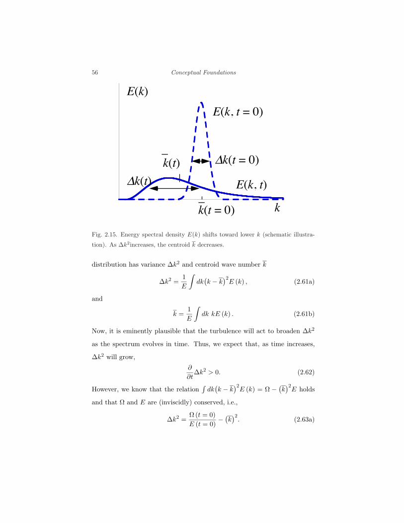
56 Conceptual Foundations
!!!""
#!!"
$
!!"" !!!"#$#%"
#!!& "#$#%"
!!"#$#%"$
!
#!!& ""
Fig. 2.15. Energy spectral density E(k) shifts toward lower k (schematic illustra-
tion). As ∆k2increases, the centroid k decreases.
distribution has variance ∆k2 and centroid wave number k
∆k2 =1E
∫dk
(k − k
)2E (k) , (2.61a)
and
k =1E
∫dk kE (k) . (2.61b)
Now, it is eminently plausible that the turbulence will act to broaden ∆k2
as the spectrum evolves in time. Thus, we expect that, as time increases,
∆k2 will grow,∂
∂t∆k2 > 0. (2.62)
However, we know that the relation∫
dk(k − k
)2E (k) = Ω −
(k)2
E holds
and that Ω and E are (inviscidly) conserved, i.e.,
∆k2 =Ω (t = 0)E (t = 0)
−(k)2
. (2.63a)

2.3 K41 Beyond Dimensional Analysis 57
Since Ω(t = 0
)/E
(t = 0
)is constant, we see that the growth of ∆k2 (Eq.(2.62))
requires∂
∂tk < 0, (2.63b)
so that the centroid of the spectrum must shift toward lower wave numbers.
This is shown in Fig.2.15. This trend is quite suggestive of the inverse
energy cascade.
We now repeat this type of exercise for the case of enstrophy. Here, it is
convenient to work with scale, not wave number. Thus, for l = 1/k, we can
define the variance
∆l2 =1Ω
∫dl
(l − l
)2Ω (l) , (2.64a)
where Ω (l) is the enstrophy density and the total enstrophy is given by
Ω =∫
dlΩ (l), and l is the enstrophy centroid scale
l =1Ω
∫dl lΩ (l) . (2.64b)
Note that convergence of the moments of Ω (l) is assumed a priori, but not
proved. Then the change of the variance is given as
∂
∂t∆l2 =
∂
∂t
1Ω
∫dl
(l − l
)2Ω (l)
=∂
∂t
1Ω
∫dl l2Ω (l)−
(l)2
.
(2.65a)
However, the integral∫
dll2Ω (l) is just the total energy, which is conserved
along with the total enstrophy. Hence,
∂
∂t∆l2 = − ∂
∂t
(l)2
. (2.65b)
For the range of scales to broaden in time (i.e., ∂∆l2/∂t > 0),
∂
∂tl < 0 (2.66)
is required, so the centroid of the distribution of enstrophy density (by scale)
must move toward smaller scale. This is suggestive of a direct cascade of

58 Conceptual Foundations
enstrophy to smaller scale. Thus, we see that the simultaneous conditions
of spectral broadening and inviscid conservation of energy and enstrophy
force the dual cascade model. In this dual cascade scenario, enstrophy is
self-similarly transferred to smaller scales while energy is self-similarly trans-
ferred to large scales.
2.3.2.2 Self-similar spectral distribution
Simple scaling arguments for the cascade spectra are then easily to con-
struct. To describe the cascade spectra, it is convenient to work with the
energy density spectrum E (k), so with a factor of k for density of states,
kE (k) has the dimension of⟨v2
⟩. Hence k3E (k) corresponds to enstro-
phy density. Spectral self-similarity leads us to hypothesis that enstrophy
cascades locally, with a rate set by the eddy-turn-over time τet for each k,
i.e.,1
τcascade=
1τet
=v (l)
l= k(kE (k))1/2. (2.67)
Then, a scale-independent enstrophy dissipation rate η = k3E (k) /τcascade
requires that(k3E (k)
)3/2 = η, (2.68a)
which immediately gives the energy spectrum for the (forward) enstrophy
cascade as
E(k) = η2/3k−3. (2.68b)
Note that the eddy-turn-over rate in the enstrophy cascade range is con-
stant in k from Eqs. (2.67) and (2.68b). The enstrophy spectrum is given
by Ω (k) = k2E (k), so that the equi-partition holds for kΩ (k) according to
Eq. (6.68b). The physics of the enstrophy cascade is successfully described
by the cartoon in Fig.2.16. This shows that stretching of iso-contours of

2.3 K41 Beyond Dimensional Analysis 59
vorticity by a turbulent flow necessarily generates smaller scale structure
in these contours, thus producing a net increase in mean square vorticity
gradient⟨(
∇∇2φ)2
⟩. The increase is what underlies the forward enstrophy
cascade process. The cascade is ultimately terminated by viscous mixing.
The forward cascade of enstrophy in k space is closely related to the homog-
enization (i.e., mixing and dissipation) of vorticity in configuration space,
to be discussed later.
Fig. 2.16. Mean square vorticity increases as vorticity isocontours stretch in a tur-
bulent flow.
The self-similar inverse cascade of energy is described correspondingly, by
balancing the energy dissipation rate ε with the flow rate of energy to larger
scale set locally by the eddy-turn-over rate, i.e., kE (k) /τcascade = ε. This
gives the relation, with the help of Eq.(2.67)
k5/2E (k)3/2 = ε, (2.69a)
so
E (k) = ε2/3k−5/3. (2.69b)
Of course, the energy cascade spectrum is the same as the K41 spectrum,
though the cascade is toward large scale. For forcing at kf , clearly here we
60 Conceptual Foundations
have
εk2f = η.
The dual cascade is represented by the schematic drawing in Fig.2.17. Note
that the inverse cascade builds up a large-scale flow from intermediate forc-
ing. The process of large-scale build-up is nicely illustrated by Fig.2.18,
which shows the evolution of the spectrum during a simulation of 2D tur-
bulence forced at intermediate scale. Ultimately, this flow occupies the
largest scale of the system, thus generating a macroscopic shear flow on
that scale. The large-scale shears can then directly strain the smaller scales,
thus breaching self-similarity and producing strong intermittency in the tur-
bulent flow.
2.3.2.3 Dispersion of particle pairs
The dispersion of particle pairs (i.e. Richardson’s problem) in a turbulent
2D flow is strongly tied to the dynamics of the dual cascades. In all cases, the
dispersion of particles separated by distance l is determined by the eddies
of that size, Eq.(2.57a), so
d
dtl = v (l) .
For the inverse cascade range, i.e., l > k−1f , Eq.(2.69b) gives v (l) = ε1/3l1/3,
so
l (t)2 ∼ ε t3, (2.70)
as in K41. Particle pairs grow super diffusively. For the forward, enstrophy
cascade range, l < k−1f , we note that the velocity v (l) = (kE (k))1/2 is given
by η1/3l, because E (k) = η2/3k−3 holds as Eq.(2.68b). We immediately

2.3 K41 Beyond Dimensional Analysis 61
ln !
ln "(!)
forcing
!f
enstrophycascade
energyinversecascade
dissipation
largescaleflow
!!"#"$!"%
#%"&'$("&
!%"&'$&
Fig. 2.17. Schematic of energy spectrum for dual cascade.
have
d
dtl = η1/3l. (2.71)
Thus, particle separation l (t) grows exponentially in time for separation
scales smaller than the forcing scale, but super diffusive growth for scales
larger than the forcing scale. The exponential divergence of particles in the
enstrophy cascade range resembles the exponential divergence of trajectories
in a stochastic system, such as for the case of overlapping resonances between
plasma particles and a spectrum of waves.

62 Conceptual Foundations
Fig. 2.18. Build-up of a large-scale flow in dual cascade [V. Borue, PRL 71 (1994)
1475]. Energy spectra normalized as (a) E (k) k3η−2/3 and (b) E (k) k5/3ε−2/3 as
the function of log10 (k/kf ) for three different parameters in simulations. (B and
C have finer resolution than A. In C, forcing occurs at finer scale than in B. See
[Borue] for details of parameters.)
2.3.2.4 Long lived vortices
It is interesting to note that long-lived coherent vortices have been observed
to emerge from decaying turbulent flows, and even in certain forced turbu-
lent flows. This important phenomenon has long been observed, but was

2.3 K41 Beyond Dimensional Analysis 63
Fig. 2.19. Vorticity contours in the initial condition (a) and long-time evolution at
a normalized time of t = 16.5 (b), where the eddy-turn-over time increases from
0.5 to 2.0 in the decay process. [J. C. McWilliams, JFM 146 (1984) 21]
dramatically emphasized by the seminal work of J. McWilliams and its off-
shoots. These studies revealed a two-stage evolution for decaying turbulence,
namely:
i) a fast stage of rapid decay and cascading, as shown in Fig.2.19(a)
ii) a second, slower stage of evolution by binary vortex interaction. In this
stage, vortices advect and strain each other, merge and sometimes form
persisting pairs. Example of this evolution is shown in Fig.2.19(b).
One of the most interesting aspects of this work is that it confirms the
intuitively appealing Okubo-Weiss criterion, which constitutes a plausible
answer (for 2D fluids) to the often-asked question of “What makes a coherent
structure coherent?”
The Okubo-Weiss criterion emerges from an asymptotic expression for the
time evolution of the local vorticity gradient ∇ρ (where ρ = ∇2φ is the local

64 Conceptual Foundations
vorticity), which predicts that
∂
∂t∇ρ =
√S2 − ρ2. (2.72)
Here, S = ∂2φ/∂x∂y is the local flow shear. The Okubo-Weiss (O-W) cri-
terion thus states that the evolution of the local vorticity gradient is set
by the Gaussian curvature of the stream function. In physical terms, the
O-W criterion states that when the magnitude of the local shear exceeds
the magnitude of local vorticity, the vorticity gradient is steeper and small
scales will develop, as they do in enstrophy cascade. If the local enstrophy
density exceeds |S|, however, the vorticity gradient will not steepen, and a
coherent vortex will simply rotate, without distortion. Locally, the flow will
be stable to the cascade process. The O-W criterion is quite plausible, as it
is consistent with the expected natural competition between shearing and
vortical circulation. Comparisons with simulations of decaying turbulence
indicate that the O-W criterion successfully predicts the location of long
lived, coherent vortices, which are, in some sense, stable to cascading, in
a turbulent flow. Indeed, when applied to a fully turbulent flow, the O-W
criterion successfully predicts the subsequent emergence and locations of co-
herent vortices after the early phase of rapid decay. Thus, the O-W criterion
constitutes one physically plausible approach to predicting intermittency in
2D turbulence.
Here, intermittency refers to breakdown of self-similar transfer by the for-
mation of stable structures. We should caution the reader that many types
of intermittency are plausible. (For instance, another origin of intermit-
tency, which is induced by the statistical variance of dissipation rate ε from
its mean 〈ε〉, is explained in [Yoshizawa, Arimitsu].) A full discussion of this
challenging, forefront problem requires a book itself.
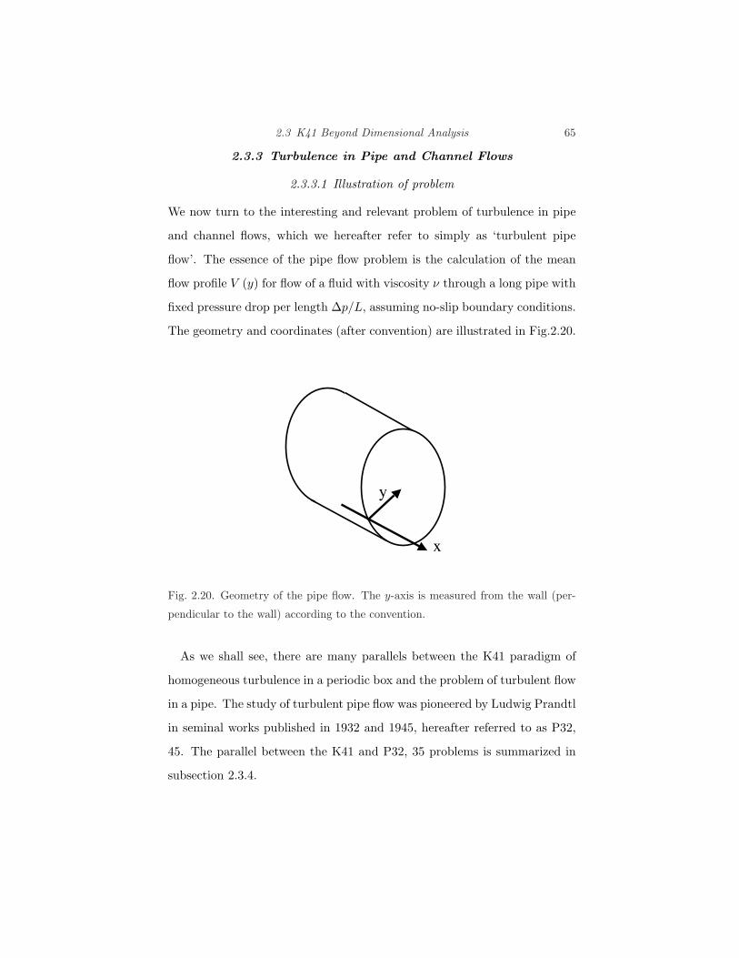
2.3 K41 Beyond Dimensional Analysis 65
2.3.3 Turbulence in Pipe and Channel Flows
2.3.3.1 Illustration of problem
We now turn to the interesting and relevant problem of turbulence in pipe
and channel flows, which we hereafter refer to simply as ‘turbulent pipe
flow’. The essence of the pipe flow problem is the calculation of the mean
flow profile V (y) for flow of a fluid with viscosity ν through a long pipe with
fixed pressure drop per length ∆p/L, assuming no-slip boundary conditions.
The geometry and coordinates (after convention) are illustrated in Fig.2.20.
!
"
Fig. 2.20. Geometry of the pipe flow. The y-axis is measured from the wall (per-
pendicular to the wall) according to the convention.
As we shall see, there are many parallels between the K41 paradigm of
homogeneous turbulence in a periodic box and the problem of turbulent flow
in a pipe. The study of turbulent pipe flow was pioneered by Ludwig Prandtl
in seminal works published in 1932 and 1945, hereafter referred to as P32,
45. The parallel between the K41 and P32, 35 problems is summarized in
subsection 2.3.4.

66 Conceptual Foundations
Like K41 turbulence, pipe flow turbulence manifests an element of univer-
sality in its phenomenology. In simple terms, pipe flow turbulence is driven
by turbulent mixing of the cross-stream shear of the mean flow dVx (y) /dy
by turbulent Reynolds stress⟨VyVx
⟩, so that turbulent energy production
P is given by:
P = −⟨VyVx
⟩ d
dyVx (y) . (2.73)
We therefore see that the turbulence is driven by the cross-stream flux of
along stream momentum. Pipe flow is perhaps the simplest example of
flux-driven turbulence, a ubiquitous paradigm with many applications to
tokamaks, solar convection, etc.
The effective drag on the flow, which opposes the driving ∆p/L, results
from turbulent transport to the pipe wall, where the no-slip boundary condi-
tion forces the stream-wise flow to vanish. Thus, turbulent transport trans-
fers or connects momentum input or drive by pressure drop to dissipation
in the viscosity dominated region close to the no-slip boundary. A cartoon
of this spatial transport process and its implications for the flow profile is
given in Fig.2.21.
2.3.3.2 Viscous sublayer
The Reynolds stress⟨VyVx
⟩is an effective measure of momentum transport
to the wall, or equivalently, the stress exerted on the wall, which we call
Tw = ρ⟨VyVx
⟩.
Here ρ indicates the mass density and Tw is the stress (not temperature).
Clearly, Tw is proportional to ∆p/L. Since there is no sink of momentum
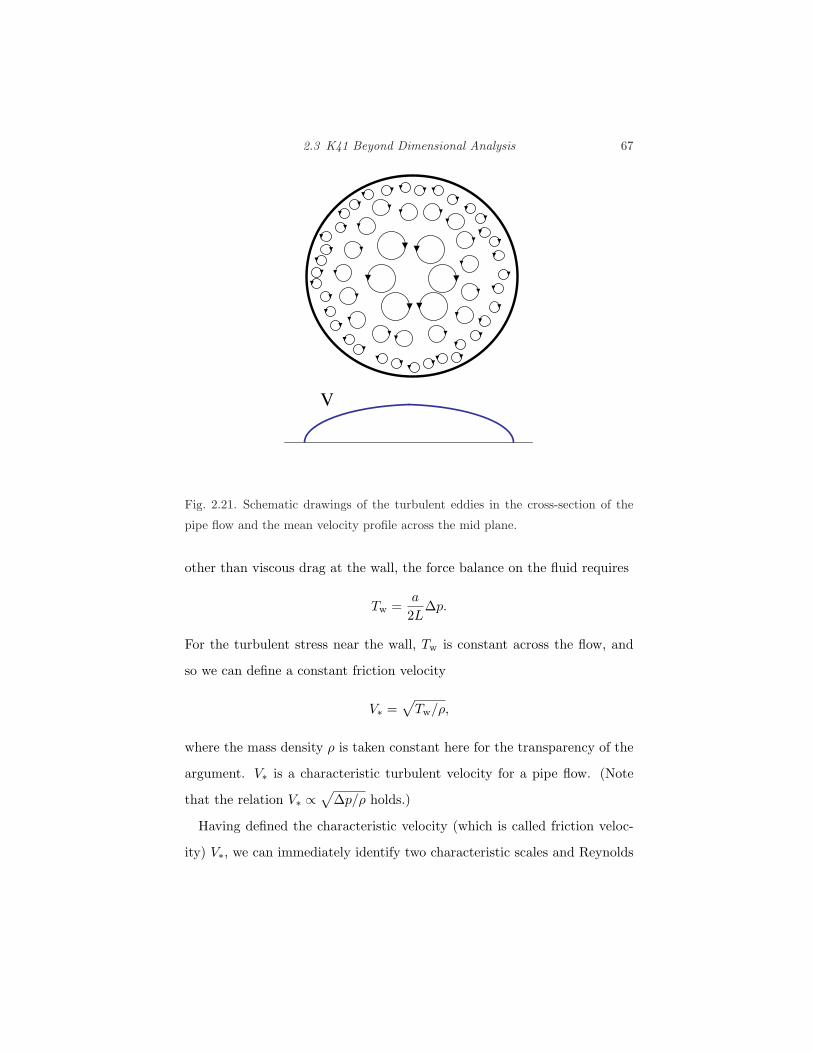
2.3 K41 Beyond Dimensional Analysis 67
!
Fig. 2.21. Schematic drawings of the turbulent eddies in the cross-section of the
pipe flow and the mean velocity profile across the mid plane.
other than viscous drag at the wall, the force balance on the fluid requires
Tw =a
2L∆p.
For the turbulent stress near the wall, Tw is constant across the flow, and
so we can define a constant friction velocity
V∗ =√
Tw/ρ,
where the mass density ρ is taken constant here for the transparency of the
argument. V∗ is a characteristic turbulent velocity for a pipe flow. (Note
that the relation V∗ ∝√
∆p/ρ holds.)
Having defined the characteristic velocity (which is called friction veloc-
ity) V∗, we can immediately identify two characteristic scales and Reynolds

68 Conceptual Foundations
numbers for pipe flow turbulence. One is the viscous sublayer width yd,
yd = νV −1∗ , (2.74)
which is a measure of the thickness of the viscosity-dominated range near
the wall. In the viscous sublayer, y < yd, the Reynolds number Re = V∗y
satisfies the relation Re < 1. In order to balance the constant wall stress
and satisfy the no-slip boundary condition at the wall, the flow profile must
be linear, i.e., V (y) ∼ V∗y/yd, in the viscous sublayer. Of course, the flow
further away from the wall is strongly turbulent, and the Reynolds number
computed with the pipe cross-section length a, Re = V∗a/ν, is much larger
than unity. Indeed, in practical applications, Re is so large that all vestiges of
the (subcritical) instability process, which initially triggered the turbulence,
have been obliterated in the fully evolved turbulent state.
2.3.3.3 Log law of the wall
As with the K41 problem, empirical observation plays a key role in defining
the problem. In the pipe flow problem, numerous experimental studies over
a broad range of turbulent flows indicate that the flow profile has a universal,
self-similar structure consisting of three layers, namely:
a) the core; i.e., y ∼ a
b) an inertial sublayer; i.e., yd < y $ a
c) the viscous sublayer; i.e., 0 < y < yd,
and that in the inertial sublayer, the flow gradient is scale independent, with
a universal structure of the form
d
dyV (y)∼V∗
y, (2.75a)

2.3 K41 Beyond Dimensional Analysis 69
so
V (y) = κV∗ ln y. (2.75b)
This logarithmic profile for the inertial sublayer flow is often referred to as
the (Prandtl) Law of the Wall, and is, to reasonable accuracy, a universal
feature of high Re pipe flow. The flow profile and the three regimes are
sketched in Fig.2.22. The empirically determined constant, κ = 0.4, is
named the von Karman constant.
!!
"!
Fig. 2.22. Mean velocity of turbulent channel flows normalized by the friction ve-
locity, U+ = V (y) /V∗ as a function of the normalized distance y+ = y/yd. Quoted
from [Yoshizawa et al. Physics of fluids 17, 075113 (2005) ], which compiled the
lines, DNS [H. Abe, et al. Int. J. Heat Fluid Flow 25, 404 (2004)] and circles,
observation [T. Wei and W. W. Willmarth, J. Fluid Mech. 204, 57 (1989) ] at
Reτ = 1016. Here, Reτ is the Reynolds number defined by use of the friction
velocity V∗. Viscous flow near wall, log law and core profile are observed.
We should mention here that though the logarithmic law of the wall profile
is the best known feature of turbulent pipe flow, it is perhaps more instruc-
tive to focus on the universality of the flow profile gradient dV (y) /dy. Note

70 Conceptual Foundations
that the local gradient is determined entirely by the distance from the wall
y (a purely local parameter!) and the friction velocity V∗. In same sense,
it is more appropriate to focus on the flow gradient instead of flow, since
the former is determined purely locally, while the flow at y is affected by
physical effects originating at points far away.
A simple, physically appealing model can be constructed to explain the
empirical law of the wall. The basic ideas of this model are:
i) turbulence intensity in the inertial sublayer is determined by a local
balance between mean profile relaxation induced by turbulent viscosity
νT and turbulent dissipation of fluctuation energy,
ii) turbulence is characterized locally by a simple velocity, namely the fric-
tion velocity V∗, and a single length scale l.
Now, turbulence energy E evolves according to a competition between
production P and dissipation ε, so
∂
∂tE = P − ε, (2.76a)
where
P = νT∂
∂yV (y) = V∗l
∂
∂yV (y) , (2.76b)
and
ε =V 3∗l
. (2.76c)
Here l is the characteristic length scale of the turbulence. Now, empirically
we have ∂V (y) /∂y = V∗/y, it follows that
∂
∂tE = V∗l
V 2∗
y2− V 3
∗l
. (2.76d)
Thus, we see that the most direct way to ensure stationality in the iner-
tial sublayer is to simply take the characteristic length scale l to be y, the

2.3 K41 Beyond Dimensional Analysis 71
distance from the wall,
l ∼ y, so νT = V∗y.
Note this ansatz ensures scale invariance in the inertial sublayer. The length
l ∼ y is often referred to as the mixing length, since by analogy with gas
kinetics where viscosity is given by thermal velocity and mean free path,
ν = vT lmfp, l ∼ y may be thought of as an effective mean free path, over
which fluid momentum is mixed by a random walk with root-mean-square
velocity V∗. In other words, the log law of the wall is based on the picture
that the length of turbulent mixing l is given by the distance from the wall
y (the upper bound by the vortex size in the region between the location y
and the wall.).
This mixing length model of pipe flow turbulence was first proposed by
Prandtl, and thus goes by the name of Prandtl Mixing Length Theory. Note
that mixing length theory also immediately recovers the logarithmic profile,
since by making the assumption of diffusive transport,
Tw
ρ=
⟨VyVx
⟩= νT
∂
∂yV (y) , (2.77a)
(note the minus sign is absorbed since y is measured from the wall) and if
νT = V∗l = V∗y, we have∂
∂yV (y) =
V∗y
. (2.77b)
2.3.3.4 Approach of self-similarity
It is enlightening to briefly review another even simpler approach to the
problem of the inertial sublayer profile, assuming similarity methods. To
this end, one can formulate the problem by noting that since it is the
mean velocity gradient which is locally determined self-similar and seem-
ingly ‘universal’, we know that the dimensionless function yV −1∗ ∂V (y) /∂y

72 Conceptual Foundations
is determined exclusively by the dimensionless parameters in the problem.
Now, since there are two characteristic length scales in pipe flow turbulence,
namely the viscous sublayer scale yd = νV −1∗ and pipe cross-section a, the
relevant dimensionless function can be written as
y
V∗
∂V (y)∂y
= F
(yd
y,y
a
). (2.78a)
For the inertial sublayer of a high Reynolds number pipe flow, y/yd #
1 and a/y # 1. Thus, assuming complete Reynolds number similarity
amounts to taking yd/y → 0 and y/a→ 0. In this limit,
y
V∗
∂V (y)∂y
= F (0, 0) → const, (2.78b)
so once again we arrive at the logarithmic Law of the Wall profile,
V (y) = κV∗ ln y. (2.78c)
Thus, we see that the Prandtl’s law of the wall emerges from extremely sim-
ple arguments of complete Reynolds number similarity and scaling methods.
The reader should note that study of corrections to the law of the wall in-
duced by incomplete similarity is ongoing and remains an active topic of
research.
2.3.4 Parallels between K41 and Prandtl’s Theory
The parallel between the K41 and P32, 35 problems was referred many
times during the discussion. At this point, the reader may wish to visit
the summary in Table 2.4, to review the many parallels between the twin
studies in self-similarity which constitute Kolmogorov’s theory of the inertial
range spectrum and Prandtl’s theory of turbulent pipe flow. This table is
largely self-explanatory. It is interesting, however, to comment on one place

2.3 K41 Beyond Dimensional Analysis 73
where a parallel does not exist, namely, in the last entry, which deals with
‘rigorous results’. For K41 theory, the ‘4/5 Law’ is a rigorous asymptotic
theorem which links the dissipation rate ε, the length scale l, and the triple
moment⟨δV 3 (l)
⟩by the relation
⟨δV 3 (l)
⟩= −4
5εl.
The 4/5 Law, derived from the Karman-Howarth relation, is perhaps the
one true theorem, which is proved in turbulence theory. Since P32,45 theory
tacitly assumes⟨δV 3 (l)
⟩∼V 3
∗ ∼εy,
it is naturally desirable to know a theorem for turbulent pipe flow, which
corresponds to the 4/5 law. Unfortunately, no such result is available at this
time.

74 Conceptual Foundations
Table 2.4. Parallel studies in self-similarity
Inertial Range Spectrum (K41) Pipe Flow Profile (P32, 45)
Basic ideas
self-similarity in scale self-similarity in space
inertial range spectrum V (l) inertial sublayer profile V (y)
eddy/wavelet mixing ‘slug’ or eddy
K41 spectrum law of the wall
Range
stirring core
inertial inertial sub-layer
dissipation viscous sub-layer
Element
l → eddy scale lM = y → mixing length
Through-put
ε→ dissipation rate V 2∗ = TW /ρ
→ wall stress, friction velocity
Rate
1/τ(l) ∼ V (l)/l (eddy turn-over) νT y−2 ∼ V∗/y (νT : eddy viscosity)
Balance
ε = V (l)2/τ(l) V 2∗ ∼νT ∂V (y)/∂y
V (l) ∼ ε1/3l1/3 ∂V (y)/∂y ∼ V∗/y → long profile
Dissipation scale length
ld = ν3/4ε−1/4 yd = νV −1∗
Fit Constant
Kolmogorov constant von Karman constant
Theorem
4/5 law ?