2 3298017( 59. 057143) 137 - Auto Recycling...
69
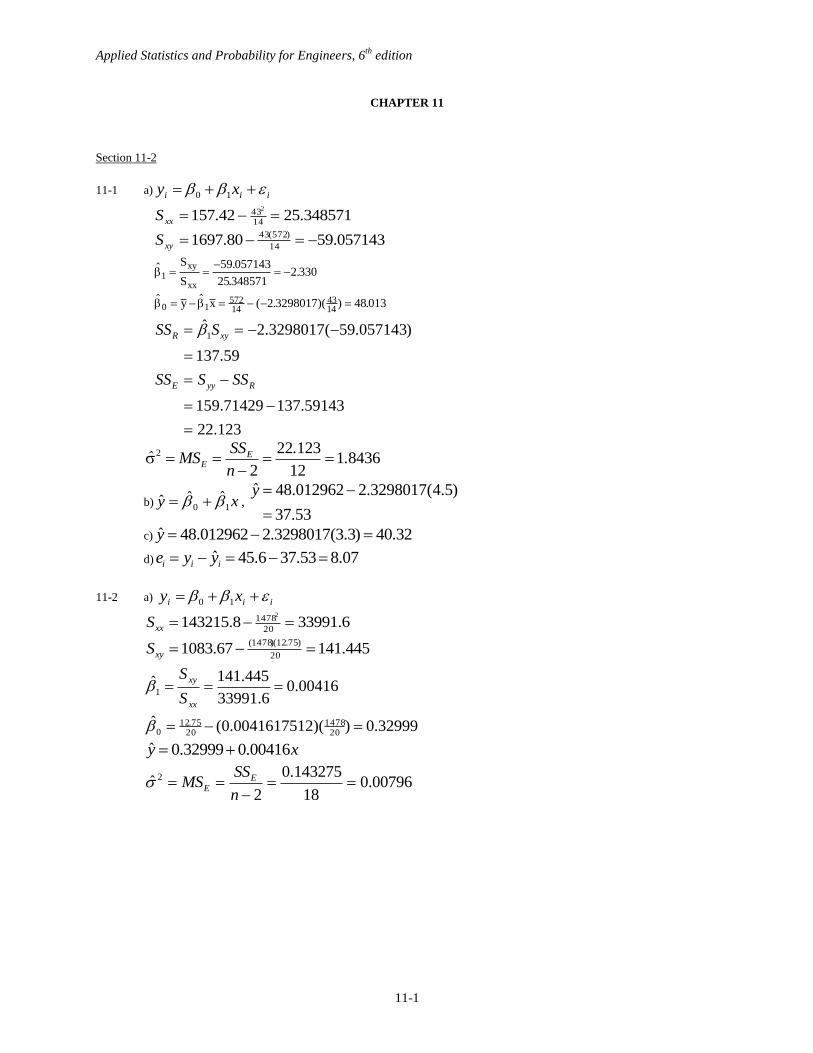
Applied Statistics and Probability for Engineers, 6 th edition 11-1 CHAPTER 11 Section 11-2 11-1 a) i i i x y 1 0 348571 . 25 42 . 157 14 43 2 xx S 057143 . 59 80 . 1697 14 ) 572 ( 43 xy S . . . ( . )( ) . 1 0 1 572 14 43 14 59 057143 25 348571 2 330 2 3298017 48 013 S S y x xy xx 123 . 22 59143 . 137 71429 . 159 59 . 137 ) 057143 . 59 ( 3298017 . 2 ˆ 1 R yy E xy R SS S SS S SS 8436 1 12 123 22 2 2 . . n SS MS ˆ E E b) x y 1 0 ˆ ˆ ˆ , 53 . 37 ) 5 . 4 ( 3298017 . 2 012962 . 48 ˆ y c) 32 . 40 ) 3 . 3 ( 3298017 . 2 012962 . 48 ˆ y d) 07 . 8 53 . 37 6 . 45 ˆ i i i y y e 11-2 a) i i i x y 1 0 6 . 33991 8 . 143215 20 1478 2 xx S 445 . 141 67 . 1083 20 ) 75 . 12 )( 1478 ( xy S 32999 . 0 ) )( 0041617512 . 0 ( ˆ 00416 . 0 6 . 33991 445 . 141 ˆ 20 1478 20 75 . 12 0 1 xx xy S S x y 00416 . 0 32999 . 0 ˆ 00796 . 0 18 143275 . 0 2 ˆ 2 n SS MS E E
Transcript of 2 3298017( 59. 057143) 137 - Auto Recycling...
Applied Statistics and Probability for Engineers, 6th
edition
11-1
CHAPTER 11
Section 11-2
11-1 a) iii xy 10
348571.2542.15714432
xxS
057143.5980.169714
)572(43xyS
.
..
( . )( ) .
1
0 157214
4314
59 057143
253485712 330
2 3298017 48 013
S
S
y x
xy
xx
123.22
59143.13771429.159
59.137
)057143.59(3298017.2ˆ1
RyyE
xyR
SSSSS
SSS
8436112
12322
2
2 ..
n
SSMSˆ E
E
b) xy 10ˆˆˆ ,
53.37
)5.4(3298017.2012962.48ˆ
y
c) 32.40)3.3(3298017.2012962.48ˆ y
d) 07.853.376.45ˆ iii yye
11-2 a) iii xy 10
6.339918.14321520
14782
xxS
445.14167.108320
)75.12)(1478(xyS
32999.0))(0041617512.0(ˆ
00416.06.33991
445.141ˆ
201478
2075.12
0
1
xx
xy
S
S
xy 00416.032999.0ˆ
00796.018
143275.0
2ˆ 2
n
SSMS E
E
Applied Statistics and Probability for Engineers, 6th
edition
11-2
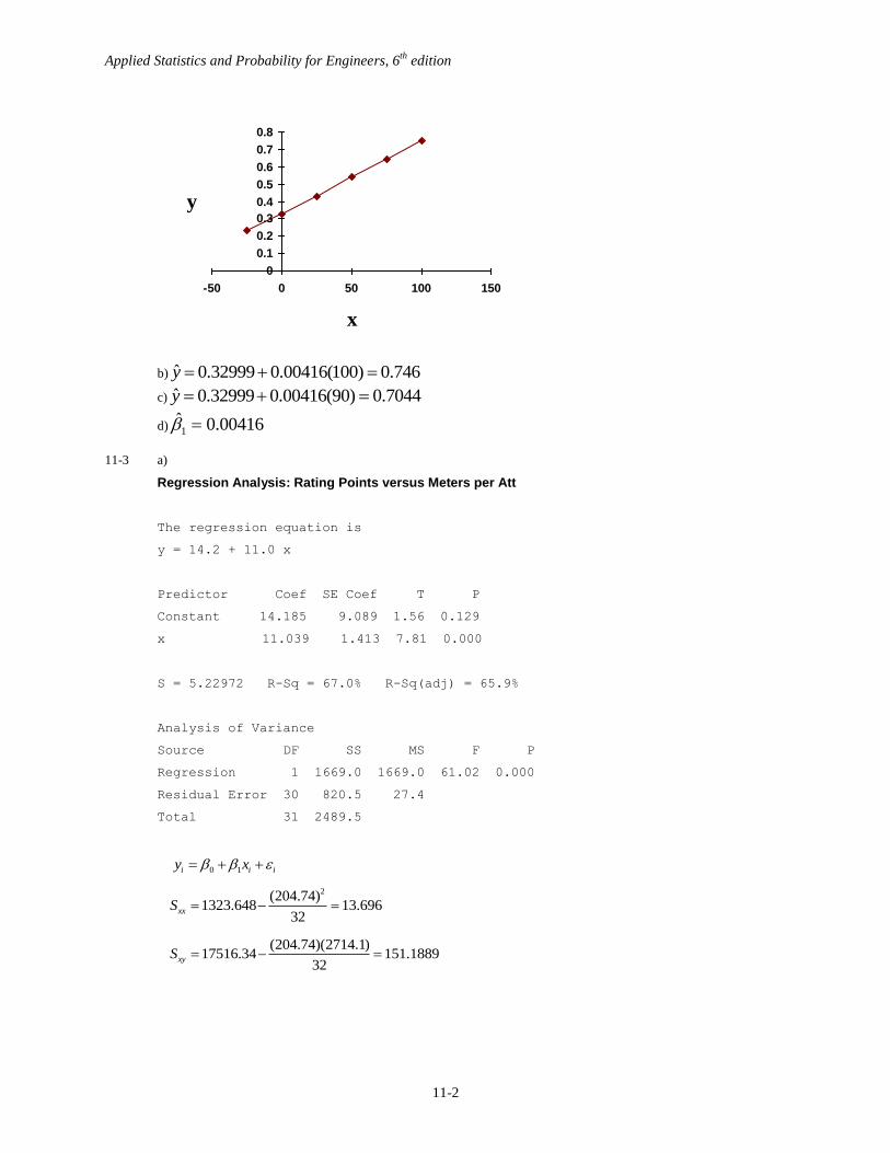
b) 746.0)100(00416.032999.0ˆ y
c) 7044.0)90(00416.032999.0ˆ y
d) 00416.0ˆ1
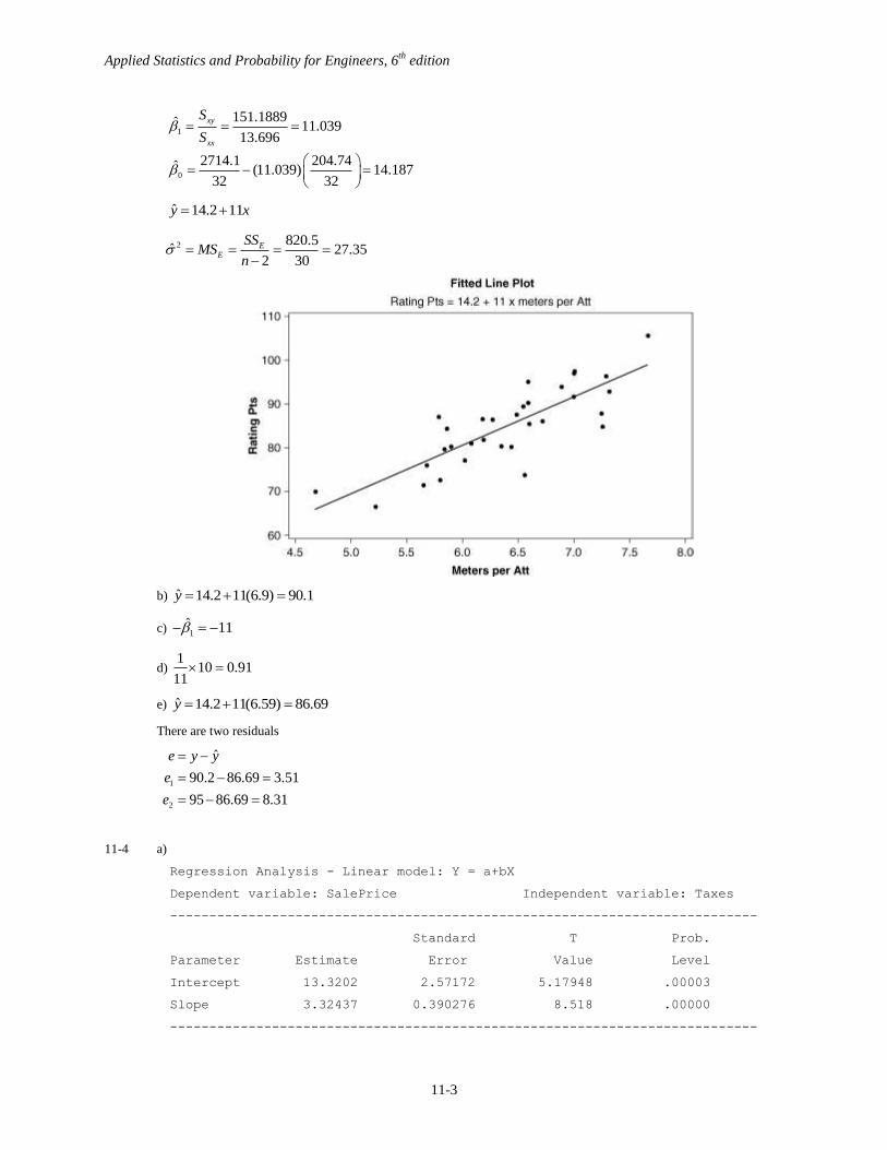
11-3 a)
Regression Analysis: Rating Points versus Meters per Att
The regression equation is
y = 14.2 + 11.0 x
Predictor Coef SE Coef T P
Constant 14.185 9.089 1.56 0.129
x 11.039 1.413 7.81 0.000
S = 5.22972 R-Sq = 67.0% R-Sq(adj) = 65.9%
Analysis of Variance
Source DF SS MS F P
Regression 1 1669.0 1669.0 61.02 0.000
Residual Error 30 820.5 27.4
Total 31 2489.5
0 1i i iy x
2(204.74)1323.648 13.696
32xxS
(204.74)(2714.1)
17516.34 151.188932
xyS
0
0.1
0.2
0.3
0.4
0.5
0.6
0.7
0.8
-50 0 50 100 150
x
y
Applied Statistics and Probability for Engineers, 6th
edition
11-3
1
0
151.1889ˆ 11.03913.696
2714.1 204.74ˆ (11.039) 14.18732 32
xy
xx
S
S
ˆ 14.2 11y x
2 820.5
ˆ 27.352 30
EE
SSMS
n
b) ˆ 14.2 11(6.9) 90.1y
c) 1ˆ 11
d) 1
10 0.9111
e) ˆ 14.2 11(6.59) 86.69y
There are two residuals
1
2
ˆ
90.2 86.69 3.51
95 86.69 8.31
e y y
e
e
11-4 a)
Regression Analysis - Linear model: Y = a+bX
Dependent variable: SalePrice Independent variable: Taxes
---------------------------------------------------------------------------
Standard T Prob.
Parameter Estimate Error Value Level
Intercept 13.3202 2.57172 5.17948 .00003
Slope 3.32437 0.390276 8.518 .00000
---------------------------------------------------------------------------
Applied Statistics and Probability for Engineers, 6th
edition
11-4
Analysis of Variance
Source Sum of Squares Df Mean Square F-Ratio Prob. Level
Model 636.15569 1 636.15569 72.5563 .00000
Residual 192.89056 22 8.76775
--------------------------------------------------------------------------
Total (Corr.) 829.04625 23
Correlation Coefficient = 0.875976 R-squared = 76.73 percent
Stnd. Error of Est. = 2.96104
2ˆ 8.76775
If the calculations were to be done by hand, use Equations (11-7) and (11-8).
ˆ 13.3202 3.32437y x
b) ˆ 13.3202 3.32437(7.3) 37.588y
c) ˆ 13.3202 3.32437(5.6039) 31.9496y
ˆ 31.9496
ˆ 28.9 31.9496 3.0496
y
e y y
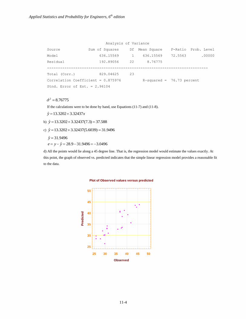
d) All the points would lie along a 45 degree line. That is, the regression model would estimate the values exactly. At
this point, the graph of observed vs. predicted indicates that the simple linear regression model provides a reasonable fit
to the data.
25 30 35 40 45 50
Observed
25
30
35
40
45
50
Pre
dic
ted
Plot of Observed values versus predicted
Applied Statistics and Probability for Engineers, 6th
edition
11-5
11-5 a)
Regression Analysis - Linear model: Y = a+bX
Dependent variable: Usage Independent variable: Temperature
----------------------------------------------------------------------------
Standard
Parameter Estimate Error T Prob.
Intercept 129.974 0.707 183.80 0.000
Slope 7.59262 0.05798 130.95 0.000
----------------------------------------------------------------------------
Analysis of Variance
Source DF Sum of Squares Mean Square F Prob. Level
Model 1 57701 57701 7148.85 0.000
Residual 10 34 3
Total 11 57734
----------------------------------------------------------------------------
Stnd. Error of Est. = 1.83431 R-Sq = 99.9%
Correlation Coefficient = 0.9999
2ˆ 3
If the calculations were to be done by hand, use Equations (11-7) and (11-8).
ˆ 130 7.59y x
b) ˆ 130 7.59(13) 228.67y
c) If monthly temperature increases by 0.5C, y increases by 7.59
d) ˆ 130 7.59(8) 190.72y
ˆ 190.72y
ˆ 192.70 190.72 1.98e y y
11-6 a) The regression equation is MPG = 39.2 - 0.0402 Engine Displacement
Predictor Coef SE Coef T P
Constant 39.156 2.006 19.52 0.000
Engine Displacement -0.040216 0.007671 -5.24 0.000
S = 3.74332 R-Sq = 59.1% R-Sq(adj) = 57.0%
Analysis of Variance
Source DF SS MS F P
Regression 1 385.18 385.18 27.49 0.000
Residual Error 19 266.24 14.01
Total 20 651.41
01.14ˆ 2
Applied Statistics and Probability for Engineers, 6th
edition
11-6
xy 0402.02.39ˆ
b) 165.32)175(0402.02.39ˆ y
c) 32.31ˆ y
08.432.314.35ˆ yye
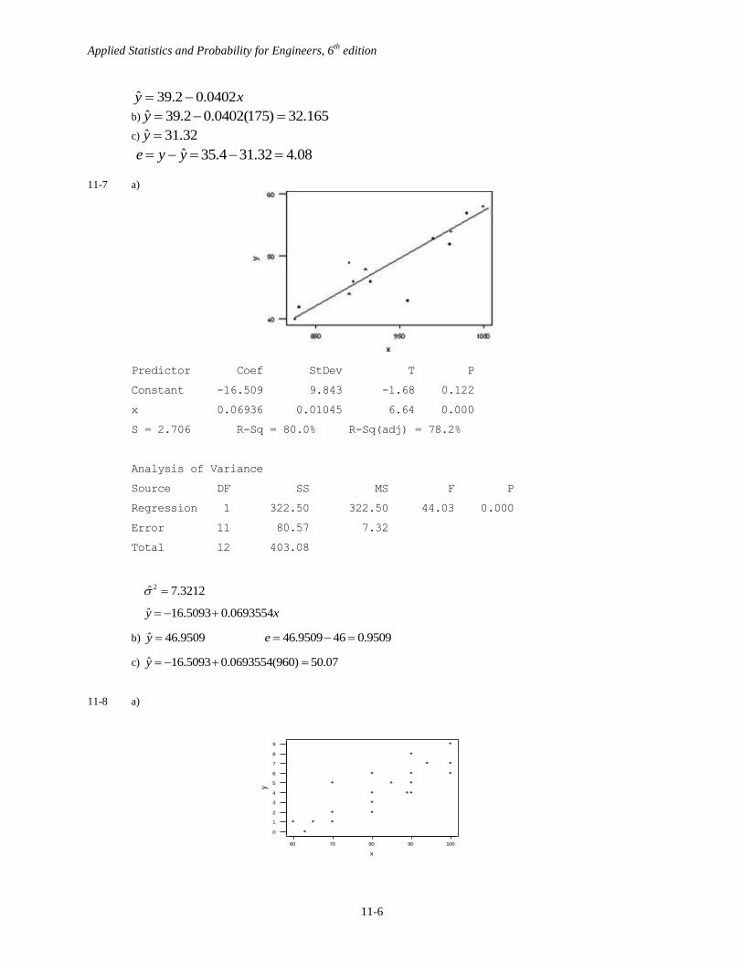
11-7 a)
Predictor Coef StDev T P
Constant -16.509 9.843 -1.68 0.122
x 0.06936 0.01045 6.64 0.000
S = 2.706 R-Sq = 80.0% R-Sq(adj) = 78.2%
Analysis of Variance
Source DF SS MS F P
Regression 1 322.50 322.50 44.03 0.000
Error 11 80.57 7.32
Total 12 403.08
2ˆ 7.3212
ˆ 16.5093 0.0693554y x
b) ˆ 46.9509y 46.9509 46 0.9509e
c) ˆ 16.5093 0.0693554(960) 50.07y
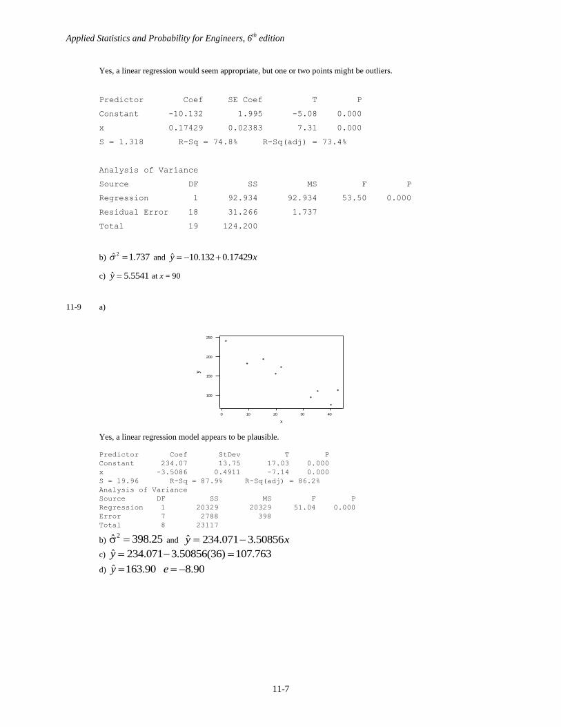
11-8 a)
10090807060
9
8
7
6
5
4
3
2
1
0
x
y
Applied Statistics and Probability for Engineers, 6th
edition
11-7
Yes, a linear regression would seem appropriate, but one or two points might be outliers.
Predictor Coef SE Coef T P
Constant -10.132 1.995 -5.08 0.000
x 0.17429 0.02383 7.31 0.000
S = 1.318 R-Sq = 74.8% R-Sq(adj) = 73.4%
Analysis of Variance
Source DF SS MS F P
Regression 1 92.934 92.934 53.50 0.000
Residual Error 18 31.266 1.737
Total 19 124.200
b) 2ˆ 1.737 and ˆ 10.132 0.17429y x
c) ˆ 5.5541y at x = 90
11-9 a)
Yes, a linear regression model appears to be plausible.
Predictor Coef StDev T P
Constant 234.07 13.75 17.03 0.000
x -3.5086 0.4911 -7.14 0.000
S = 19.96 R-Sq = 87.9% R-Sq(adj) = 86.2%
Analysis of Variance
Source DF SS MS F P
Regression 1 20329 20329 51.04 0.000
Error 7 2788 398
Total 8 23117
b) 25.398ˆ 2 and xy 50856.3071.234ˆ
c) 763.107)36(50856.3071.234ˆ y
d) 90.890.163ˆ ey
403020100
250
200
150
100
x
y

Applied Statistics and Probability for Engineers, 6th
edition
11-8
11-10 a)
Yes, a simple linear regression model seems appropriate for these data.
Predictor Coef StDev T P
Constant 0.470 1.936 0.24 0.811
x 20.567 2.142 9.60 0.000
S = 3.716 R-Sq = 85.2% R-Sq(adj) = 84.3%
Analysis of Variance
Source DF SS MS F P
Regression 1 1273.5 1273.5 92.22 0.000
Error 16 220.9 13.8
Total 17 1494.5
b) 2ˆ 13.81
ˆ 0.470467 20.5673y x
c) ˆ 0.470467 20.5673(1) 21.038y
d) ˆ 13.42787 2.5279 for 0.63y e x
11-11 a)
1.81.61.41.21.00.80.60.40.20.0
40
30
20
10
0
x
y

Applied Statistics and Probability for Engineers, 6th
edition
11-9
Yes, a simple linear regression (straight-line) model seems plausible for this situation.
Predictor Coef SE Coef T P
Constant 18090.2 310.8 58.20 0.000
x -254.55 20.34 -12.52 0.000
S = 678.964 R-Sq = 89.7% R-Sq(adj) = 89.1%
Analysis of Variance
Source DF SS MS F P
Regression 1 72222688 72222688 156.67 0.000
Residual Error 18 8297849 460992
Total 19 80520537
b) 2ˆ 460992
ˆ 18090.2 254.55y x
c) ˆ 18090.2 254.55(20) 12999.2y
d) If there were no error, the values would all lie along the 45 line. The plot indicates age is a reasonable regressor
variable.
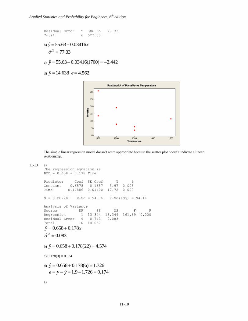
11-12 a) The regression equation is
Porosity = 55.6 - 0.0342 Temperature
Predictor Coef SE Coef T P
Constant 55.63 32.11 1.73 0.144
Temperature -0.03416 0.02569 -1.33 0.241
S = 8.79376 R-Sq = 26.1% R-Sq(adj) = 11.3%
Analysis of Variance
Source DF SS MS F P
Regression 1 136.68 136.68 1.77 0.241
Applied Statistics and Probability for Engineers, 6th
edition
11-10
Residual Error 5 386.65 77.33
Total 6 523.33
b) xy 03416.063.55ˆ
33.77ˆ 2
c) 442.2)1700(03416.063.55ˆ y
d) 638.14ˆ y 562.4e
The simple linear regression model doesn’t seem appropriate because the scatter plot doesn’t indicate a linear
relationship.
11-13 a)
The regression equation is BOD = 0.658 + 0.178 Time
Predictor Coef SE Coef T P
Constant 0.6578 0.1657 3.97 0.003
Time 0.17806 0.01400 12.72 0.000
S = 0.287281 R-Sq = 94.7% R-Sq(adj) = 94.1%
Analysis of Variance
Source DF SS MS F P
Regression 1 13.344 13.344 161.69 0.000
Residual Error 9 0.743 0.083
Total 10 14.087
xy 178.0658.0ˆ
083.0ˆ 2
b) 574.4)22(178.0658.0ˆ y
c) 0.178(3) = 0.534
d) 726.1)6(178.0658.0ˆ y
174.0726.19.1ˆ yye
e)
Temperature
Po
rosit
y
15001400130012001100
30
25
20
15
10
5
0
Scatterplot of Porosity vs Temperature

Applied Statistics and Probability for Engineers, 6th
edition
11-11
All the points would lie along the 45 degree line yy ˆ . That is, the regression model would estimate the values
exactly. At this point, the graph of observed vs. predicted indicates that the simple linear regression model provides a
reasonable fit to the data.
11-14 a)
The regression equation is
Deflection = 32.0 - 0.277 Stress level
Predictor Coef SE Coef T P
Constant 32.049 2.885 11.11 0.000
Stress level -0.27712 0.04361 -6.35 0.000
S = 1.05743 R-Sq = 85.2% R-Sq(adj) = 83.1%
Analysis of Variance
Source DF SS MS F P
Regression 1 45.154 45.154 40.38 0.000
Residual Error 7 7.827 1.118
Total 8 52.981
2ˆ 1.118
y
y-h
at
4.03.53.02.52.01.51.00.5
4.5
4.0
3.5
3.0
2.5
2.0
1.5
1.0
Scatterplot of y-hat vs y
Applied Statistics and Probability for Engineers, 6th
edition
11-12
b) ˆ 32.05 0.277(64) 14.322y
c) (0.277)(5) = 1.385
d) 1
3.610.277
e) ˆ 32.05 0.277(75) 11.275y ˆ 12.534 11.275 1.259e y y
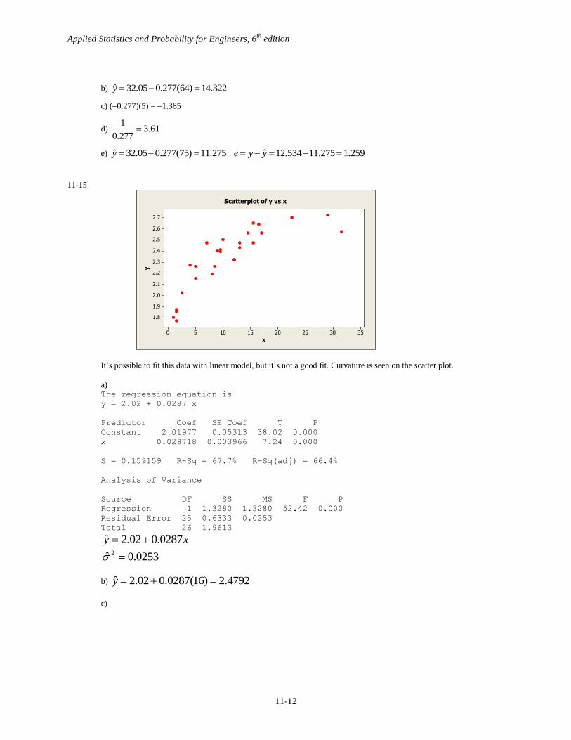
11-15
It’s possible to fit this data with linear model, but it’s not a good fit. Curvature is seen on the scatter plot.
a) The regression equation is
y = 2.02 + 0.0287 x
Predictor Coef SE Coef T P
Constant 2.01977 0.05313 38.02 0.000
x 0.028718 0.003966 7.24 0.000
S = 0.159159 R-Sq = 67.7% R-Sq(adj) = 66.4%
Analysis of Variance
Source DF SS MS F P
Regression 1 1.3280 1.3280 52.42 0.000
Residual Error 25 0.6333 0.0253
Total 26 1.9613
xy 0287.002.2ˆ
0253.0ˆ 2
b) 4792.2)16(0287.002.2ˆ y
c)
x
y
35302520151050
2.7
2.6
2.5
2.4
2.3
2.2
2.1
2.0
1.9
1.8
Scatterplot of y vs x
Applied Statistics and Probability for Engineers, 6th
edition
11-13
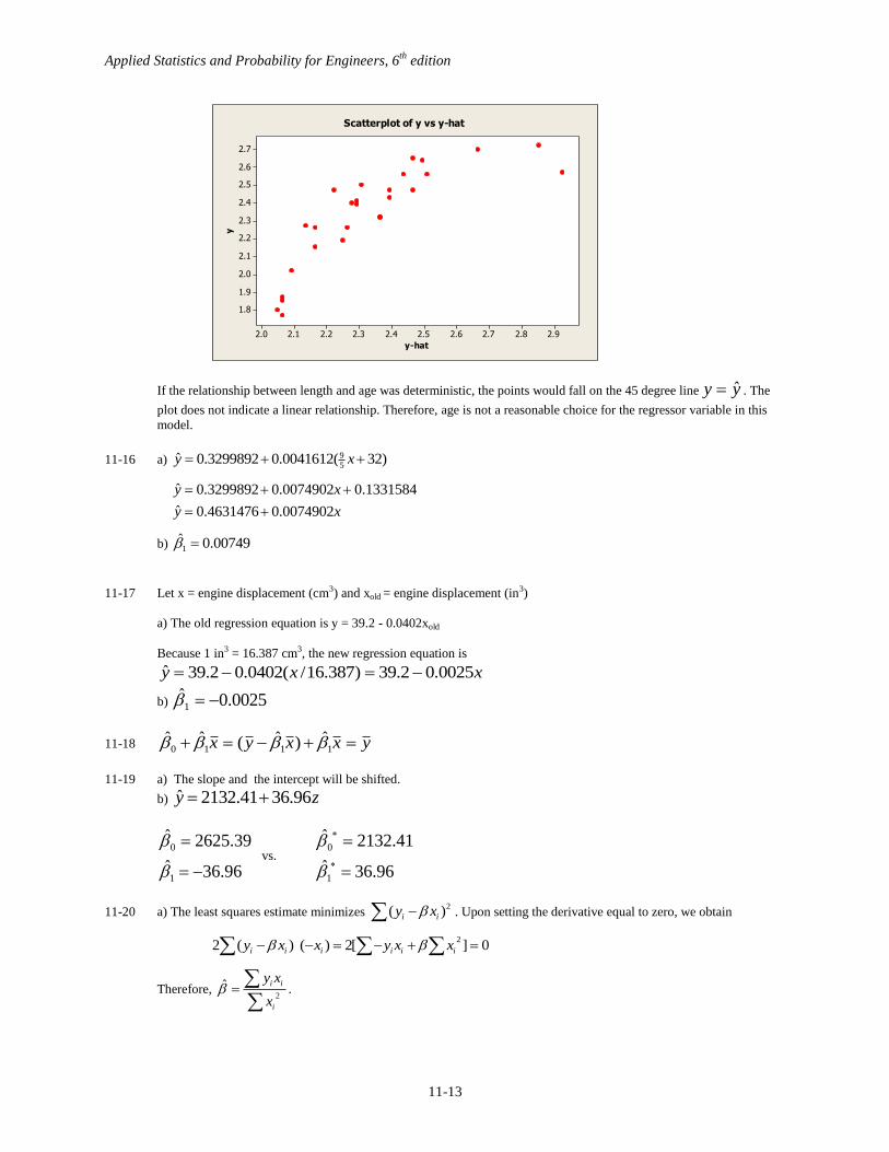
If the relationship between length and age was deterministic, the points would fall on the 45 degree line yy ˆ . The
plot does not indicate a linear relationship. Therefore, age is not a reasonable choice for the regressor variable in this
model.
11-16 a) 9
5ˆ 0.3299892 0.0041612( 32)y x
ˆ 0.3299892 0.0074902 0.1331584
ˆ 0.4631476 0.0074902
y x
y x
b) 1ˆ 0.00749
11-17 Let x = engine displacement (cm3) and xold = engine displacement (in3)
a) The old regression equation is y = 39.2 - 0.0402xold
Because 1 in3 = 16.387 cm3, the new regression equation is
xxy 0025.02.39)387.16/(0402.02.39ˆ
b) 0025.0ˆ1
11-18 yxxyx 1110ˆ)ˆ(ˆˆ
11-19 a) The slope and the intercept will be shifted.
b) zy 96.3641.2132ˆ
96.36ˆ
39.2625ˆ
1
0
vs.
96.36ˆ
41.2132ˆ
1
0
11-20 a) The least squares estimate minimizes 2( )i iy x . Upon setting the derivative equal to zero, we obtain
2
2 ( ) ( ) 2[ ] 0i i i i i iy x x y x x
Therefore, 2
ˆ i i
i
y x
x
.
y-hat
y
2.92.82.72.62.52.42.32.22.12.0
2.7
2.6
2.5
2.4
2.3
2.2
2.1
2.0
1.9
1.8
Scatterplot of y vs y-hat
Applied Statistics and Probability for Engineers, 6th
edition
11-14
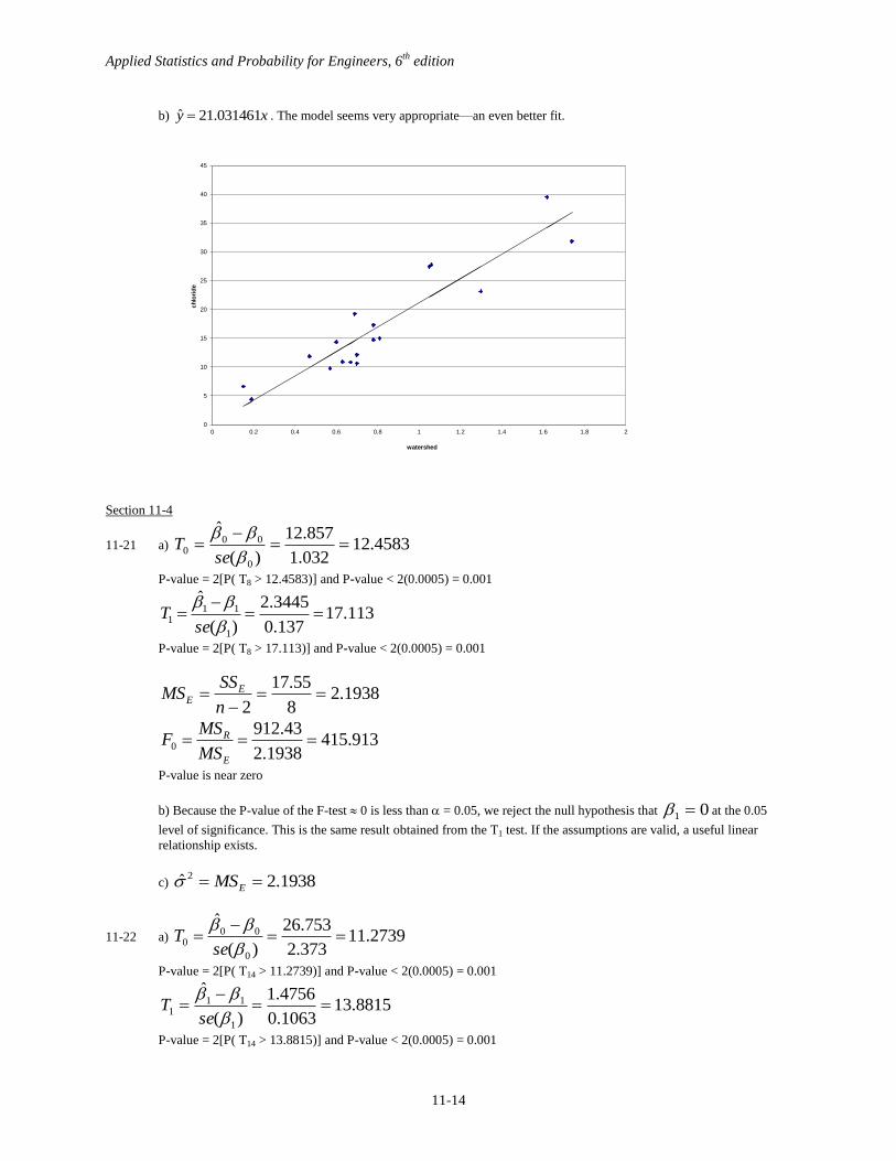
b) ˆ 21.031461y x . The model seems very appropriate—an even better fit.
Section 11-4
11-21 a) 4583.12032.1
857.12
)(
ˆ
0
000
seT
P-value = 2[P( T8 > 12.4583)] and P-value < 2(0.0005) = 0.001
113.17137.0
3445.2
)(
ˆ
1
111
seT
P-value = 2[P( T8 > 17.113)] and P-value < 2(0.0005) = 0.001
1938.28
55.17
2
n
SSMS E
E
913.4151938.2
43.9120
E
R
MS
MSF
P-value is near zero
b) Because the P-value of the F-test 0 is less than = 0.05, we reject the null hypothesis that 01 at the 0.05
level of significance. This is the same result obtained from the T1 test. If the assumptions are valid, a useful linear
relationship exists.
c) 1938.2ˆ 2 EMS
11-22 a) 2739.11373.2
753.26
)(
ˆ
0
000
seT
P-value = 2[P( T14 > 11.2739)] and P-value < 2(0.0005) = 0.001
8815.131063.0
4756.1
)(
ˆ
1
111
seT
P-value = 2[P( T14 > 13.8815)] and P-value < 2(0.0005) = 0.001
0
5
10
15
20
25
30
35
40
45
0 0.2 0.4 0.6 0.8 1 1.2 1.4 1.6 1.8 2
ch
lori
de
watershed
Applied Statistics and Probability for Engineers, 6th
edition
11-15
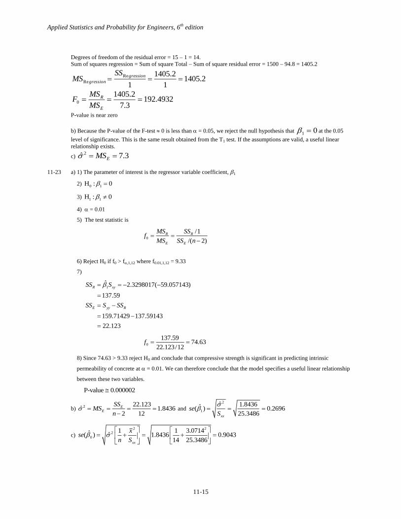
Degrees of freedom of the residual error = 15 – 1 = 14.
Sum of squares regression = Sum of square Total – Sum of square residual error = 1500 – 94.8 = 1405.2
2.14051
2.1405
1
Re
Re gression
gression
SSMS
4932.1923.7
2.14050
E
R
MS
MSF
P-value is near zero
b) Because the P-value of the F-test 0 is less than = 0.05, we reject the null hypothesis that 01 at the 0.05
level of significance. This is the same result obtained from the T1 test. If the assumptions are valid, a useful linear
relationship exists.
c) 3.7ˆ 2 EMS
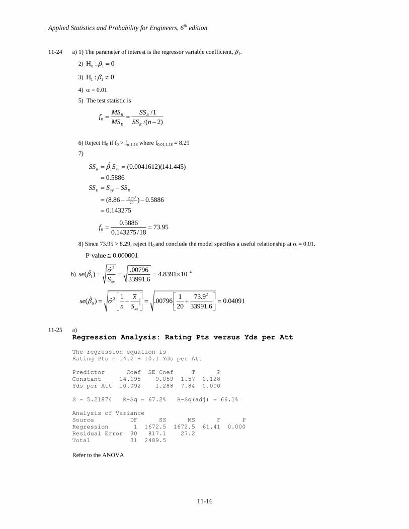
11-23 a) 1) The parameter of interest is the regressor variable coefficient, 1
2) 0 1H : 0
3) 1 1H : 0
4) = 0.01
5) The test statistic is
0
/1
/( 2)
R R
E E
MS SSf
MS SS n
6) Reject H0 if f0 > f,1,12 where f0.01,1,12 = 9.33
7)
1ˆ 2.3298017( 59.057143)
137.59
159.71429 137.59143
22.123
R xy
E yy R
SS S
SS S SS
0
137.5974.63
22.123/12f
8) Since 74.63 > 9.33 reject H0 and conclude that compressive strength is significant in predicting intrinsic
permeability of concrete at = 0.01. We can therefore conclude that the model specifies a useful linear relationship
between these two variables.
P-value 0.000002
b) 2 22.123
ˆ 1.84362 12
EE
SSMS
n
and
2
1
ˆ 1.8436ˆ( ) 0.269625.3486xx
seS
c)
2 22
0
1 1 3.0714ˆ ˆ( ) 1.8436 0.904314 25.3486xx
xse
n S
Applied Statistics and Probability for Engineers, 6th
edition
11-16
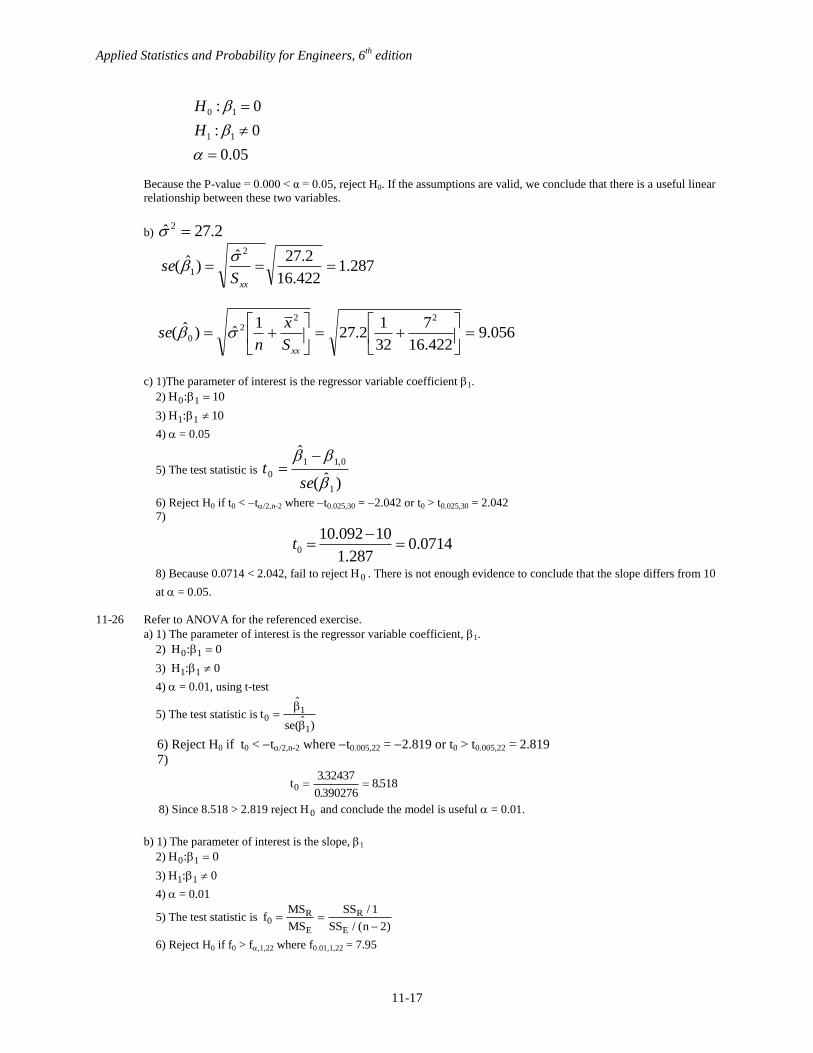
11-24 a) 1) The parameter of interest is the regressor variable coefficient, 1.
2) 0 1H : 0
3) 1 1H : 0
4) = 0.01
5) The test statistic is
0
/1
/( 2)
R R
E E
MS SSf
MS SS n
6) Reject H0 if f0 > f,1,18 where f0.01,1,18 = 8.29
7)
2
1
12.75
20
ˆ (0.0041612)(141.445)
0.5886
(8.86 ) 0.5886
0.143275
R xy
E yy R
SS S
SS S SS
0
0.588673.95
0.143275/18f
8) Since 73.95 > 8.29, reject H0 and conclude the model specifies a useful relationship at = 0.01.
P-value 0.000001
b)
24
1
ˆ .00796ˆ( ) 4.8391 1033991.6xx
seS
22
0
1 1 73.9ˆ ˆ( ) .00796 0.0409120 33991.6xx
xse
n S
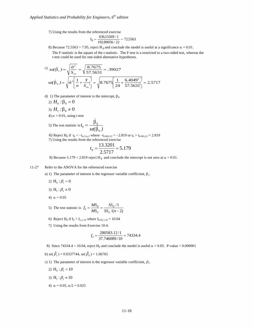
11-25 a)
Regression Analysis: Rating Pts versus Yds per Att
The regression equation is
Rating Pts = 14.2 + 10.1 Yds per Att
Predictor Coef SE Coef T P
Constant 14.195 9.059 1.57 0.128
Yds per Att 10.092 1.288 7.84 0.000
S = 5.21874 R-Sq = 67.2% R-Sq(adj) = 66.1%
Analysis of Variance
Source DF SS MS F P
Regression 1 1672.5 1672.5 61.41 0.000
Residual Error 30 817.1 27.2
Total 31 2489.5
Refer to the ANOVA
Applied Statistics and Probability for Engineers, 6th
edition
11-17
05.0
0:
0:
11
10
H
H
Because the P-value = 0.000 < α = 0.05, reject H0. If the assumptions are valid, we conclude that there is a useful linear
relationship between these two variables.
b) 2.27ˆ 2
287.1422.16
2.27ˆ)ˆ(
2
1 xxS
se
056.9422.16
7
32
12.27
1ˆ)ˆ(
222
0
xxS
x
nse
c) 1)The parameter of interest is the regressor variable coefficient 1.
2) H0 1 10:
3) H1 1 10:
4) = 0.05
5) The test statistic is
)ˆ(
ˆ
1
0,11
0
set
6) Reject H0 if t0 < t/2,n-2 where t0.025,30 = 2.042 or t0 > t0.025,30 = 2.042
7)
0714.0287.1
10092.100
t
8) Because 0.0714 < 2.042, fail to reject H 0 . There is not enough evidence to conclude that the slope differs from 10
at = 0.05.
11-26 Refer to ANOVA for the referenced exercise.
a) 1) The parameter of interest is the regressor variable coefficient, 1.
2) H0 1 0:
3) H1 1 0:
4) = 0.01, using t-test
5) The test statistic is tse
01
1
( )
6) Reject H0 if t0 < t/2,n-2 where t0.005,22 = 2.819 or t0 > t0.005,22 = 2.819
7)
t0
332437
0 3902768518
.
..
8) Since 8.518 > 2.819 reject H 0 and conclude the model is useful = 0.01.
b) 1) The parameter of interest is the slope, 1
2) H0 1 0:
3) H1 1 0:
4) = 0.01
5) The test statistic is fMS
MS
SS
SS n
R
E
R
E0
1
2
/
/ ( )
6) Reject H0 if f0 > f,1,22 where f0.01,1,22 = 7.95
Applied Statistics and Probability for Engineers, 6th
edition
11-18
7) Using the results from the referenced exercise
f0
63615569 1
192 89056 2272 5563
. /
. /.
8) Because 72.5563 > 7.95, reject H 0 and conclude the model is useful at a significance = 0.01.
The F-statistic is the square of the t-statistic. The F-test is a restricted to a two-sided test, whereas the
t-test could be used for one-sided alternative hypotheses.
c) 39027563157
767582
1 ..
.
S
ˆ)ˆ(se
xx
57172563157
40496
24
176758
1 22
0 ..
..
S
x
nˆ)ˆ(se
xx
d) 1) The parameter of interest is the intercept, 0.
2) 000 :H
3) 001 :H
4) = 0.01, using t-test
5) The test statistic is)ˆ(se
ˆt
0
00
6) Reject H0 if t0 < t/2,n-2 where t0.005,22 = 2.819 or t0 > t0.005,22 = 2.819
7) Using the results from the referenced exercise
179.55717.2
3201.130 t
8) Because 5.179 > 2.819 reject H 0 and conclude the intercept is not zero at = 0.01.
11-27 Refer to the ANOVA for the referenced exercise
a) 1) The parameter of interest is the regressor variable coefficient, 1.
2) 0 1H : 0
3) 1 1H : 0
4) = 0.05
5) The test statistic is 0
/1
/( 2)
R R
E E
MS SSf
MS SS n
6) Reject H0 if f0 > f,1,10 where f0.05,1,10 = 10.04
7) Using the results from Exercise 10-6
0
280583.12 /174334.4
37.746089 /10f
8) Since 74334.4 > 10.04, reject H0 and conclude the model is useful = 0.05. P-value < 0.000001
b) se( 1 ) = 0.0337744, se( 0 ) = 1.66765
c) 1) The parameter of interest is the regressor variable coefficient, 1.
2) 0 1H : 10
3) 1 1H : 10
4) = 0.05, /2 = 0.025

Applied Statistics and Probability for Engineers, 6th
edition
11-19
5) The test statistic is 1 1,0
0
1
ˆ
ˆ( )t
se
6) Reject H0 if t0 < t/2,n-2 where t0.025,10 = 2.228 or t0 > t0.025,10 = 2.228
7) Using the results from Exercise 10-6
0
9.21 1023.37
0.0338t
8) Since 23.37 < 2.228 reject H0 and conclude the slope is not 10 at = 0.05. P-value ≈ 0.
d) H0: 0 = 0 H1: 0 0
0
6.3355 03.8
1.66765t
P-value < 0.005. Reject H0 and conclude that the intercept should be included in the model.
11-28 Refer to the ANOVA for the referenced exercise.
0: 10 H , 011 :H
a)
19,1,05.00
19,1,05.0
0
38.4
49.2701.14
18.385
ff
f
MS
MSf
E
R
Reject the null hypothesis and conclude that the slope is not zero. The P-value ≈ 0.
b) From the computer output in the referenced exercise
006.2)( 0 se , 007671.0)( 1 se
c)
0 1 1 1
1 1,0
0
1
0.01,19 0 0.01,19 0
: 0.05; : 0.05
ˆ ˆ 0.040216 ( 0.05) 0.09021611.76
ˆ 0.007671 0.007671( )
2.539, since is not less than - 2.539, do not reject
1.0
H H
tse
t t t H
P
d)
0 0 1 0
0 0,0
0
0
0.005,19 0 0.005,19 0
: 0; : 0
ˆ ˆ 39.156 019.52
ˆ 2.006( )
2.861, since | | > reject
4.95 14 0
H H
tse
t t t H
P E
Applied Statistics and Probability for Engineers, 6th
edition
11-20
11-29 Refer to the ANOVA for the referenced exercise.
a) 0: 10 H
011 :H
= 0.05
11,1,01.00
11,1,01.0
0
65.9
0279.44
ff
f
f
Therefore, reject H0. P-value ≈ 0
b) 010452401 .)ˆ(se
8434690 .)ˆ(se
c) 000 :H
001 :H
= 0.05
1120
11025
0
2012
677181
,/
,.
t|t|
.t
.t
Therefore, fail to reject H0. P-value = 0.122
11-30 Refer to the ANOVA for the referenced exercise
a) 010 :H
011 :H
= 0.05
18,1,0
18,1,05.0
0
414.4
53.50
ff
f
f
Therefore, reject H0. P-value ≈ 0
b) 025661301 .)ˆ(se
1352620 .)ˆ(se
c) 000 :H
001 :H
= 0.05
18,2/0
18,025.
0
||
101.2
5.079-
tt
t
t
Therefore, reject H0. P-value ≈ 0
11-31 Refer to ANOVA for the referenced exercise
a) 010 :H
011 :H
= 0.05

Applied Statistics and Probability for Engineers, 6th
edition
11-21
18,1,05.00
18,1,05.0
0
41.4
2.155
ff
f
f
Therefore, reject H0. P-value < 0.00001
b) 3468451 .)ˆ(se
9668120 .)ˆ(se
c) 3010 :H
3011 :H
= 0.01
18,2/0
18,005.
0
||
878.2
3466.296681.2
)30(9618.36
tt
t
t
Therefore, fail to reject H0. P-value = 0.0153(2) = 0.0306
d) 000 :H
001 :H
= 0.01
878.2
8957.57
18,005.0
0
t
t
t t0 218 / , , therefore, reject H0. P-value < 0.00001
e) H0 0 2500:
250001 :H
= 0.01
552.2
7651.23468.45
250039.2625
18,01.
0
t
t
18,0 tt , therefore reject H0 . P-value = 0.0064
11-32 Refer to ANOVA for the referenced exercise
a) 0 1H : 0
1 1H : 0
= 0.05
0
0.05,1,16
0 ,1,16
92.224
4.49
f
f
f f
Therefore, reject H0.
b) P-value < 0.00001
c) 1ˆ( ) 2.14169se
Applied Statistics and Probability for Engineers, 6th
edition
11-22
0ˆ( ) 1.93591se
d) 0 0H : 0
1 0H : 0
= 0.05
0
0.025,16
0 / 2,16
0.243
2.12
t
t
t t
Therefore, do not reject H0. There is not sufficient evidence to conclude that the intercept differs from zero. Based on
this test result, the intercept could be removed from the model.
11-33 a) Refer to the ANOVA from the referenced exercise.
05.0
0:
0:
11
10
H
H
Because the P-value = 0.000 < α = 0.05, reject H0. There is evidence of a linear relationship between these two
variables.
b) 083.0ˆ 2
The standard errors for the parameters can be obtained from the computer output or calculated as follows.
014.091.420
083.0ˆ)ˆ(
2
1 xxS
se
1657.091.420
09.10
11
1083.0
1ˆ)ˆ(
222
0
xxS
x
nse
c)
1) The parameter of interest is the intercept β0.
2) 0: 00 H
3) 0: 01 H
4) 05.0
5) The test statistic is )( 0
0
0
set
6) Reject H0 if 2,2/0 ntt where 262.29,025.0 t or 2,2/0 ntt where 262.29,025.0 t
7) Using the results from the referenced exercise
97.31657.0
6578.00 t
8) Because t0 = 3.97 > 2.262 reject H0 and conclude the intercept is not zero at α = 0.05.
11-34 a) Refer to the ANOVA for the referenced exercise.
05.0
0:
0:
11
10
H
H
Applied Statistics and Probability for Engineers, 6th
edition
11-23
Because the P-value = 0.000 < α = 0.05, reject H0. There is evidence of a linear relationship between these two
variables.
b) Yes
c) 118.1ˆ 2
0436.0588
118.1ˆ)ˆ(
2
1 xxS
se
885.2588
67.65
9
1118.1
1ˆ)ˆ(
222
0
xxS
x
nse
11-35 a) 0 1H : 0
1 1H : 0
α 0.01
Because the P-value = 0.310 > = 0.01, fail to reject H0. There is not sufficient evidence of a linear relationship
between these two variables.
The regression equation is
BMI = 13.8 + 0.256 Age
Predictor Coef SE Coef T P
Constant 13.820 9.141 1.51 0.174
Age 0.2558 0.2340 1.09 0.310
S = 5.53982 R-Sq = 14.6% R-Sq(adj) = 2.4%
Analysis of Variance
Source DF SS MS F P
Regression 1 36.68 36.68 1.20 0.310
Residual Error 7 214.83 30.69
Total 8 251.51
b) 2
1 0ˆ ˆˆ 30.69, ( ) 0.2340, ( ) 9.141se se from the computer output
c)
2 22
0
1 1 38.256ˆ ˆ( ) 30.69 9.1419 560.342xx
xse
n S
Applied Statistics and Probability for Engineers, 6th
edition
11-24
11-36
xxSt
/ˆ
ˆ
2
10
After the transformation 11
ˆˆ a
b
, xxxx SaS 2,
00ˆˆ, bxax
, and
ˆˆ b. Therefore,
022
10
/)ˆ(
/ˆt
Sab
abt
xx
.
11-37 331.0422.16/315.5
|)5.12(10|
d
Assume = 0.05, from Chart VIIe and interpolating between the curves for n = 30 and n = 40, 55.0
11-38 a) 2
2
ˆ
ˆ
ix
has a t distribution with n 1 degree of freedom.
b) From Exercise 11-15, ˆ ˆ21.031461, 3.611768, and 2 14.7073ix .
The t-statistic in part (a) is 22.3314 and 0 0H : 0 is rejected at usual values.
Sections 11-5 and 11-6
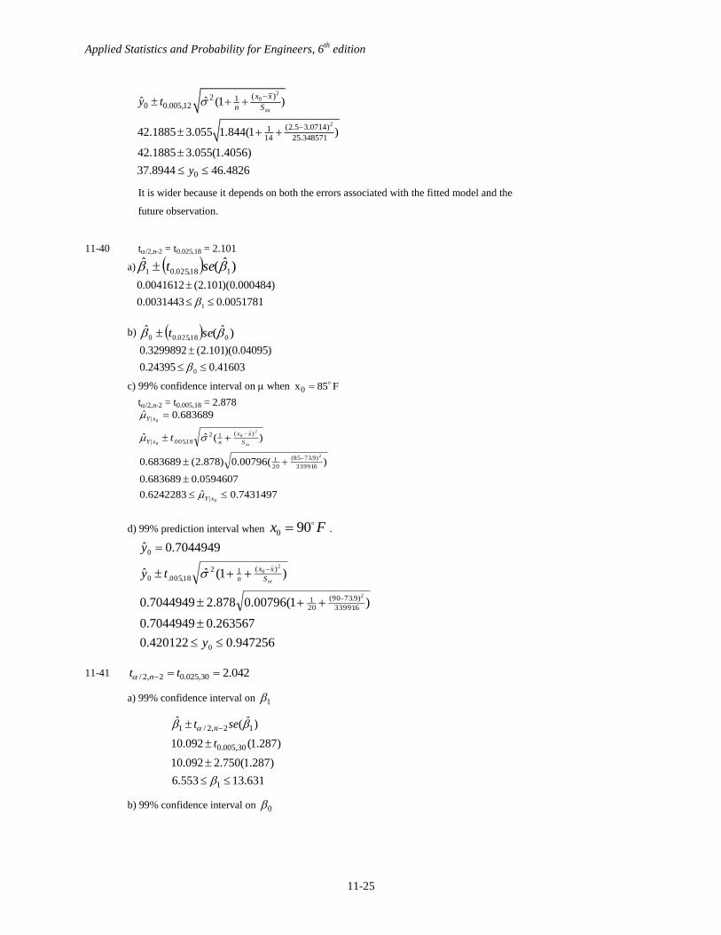
11-39 t/2,n-2 = t0.025,12 = 2.179
a) 95% confidence interval on 1 .
1 / 2, 2 1
.025,12
1
ˆ ˆ( )
2.3298 (0.2696)
2.3298 2.179(0.2696)
2.9173. 1.7423.
nt se
t
b) 95% confidence interval on 0 .
0 .025,12 0
0
ˆ ˆ( )
48.0130 2.179(0.5959)
46.7145 49.3115.
t se
c) 95% confidence interval on when x0 2 5 . .
0
20
0
2
0
|
( )2 1| .025,12
(2.5 3.0714)114 25.3486
|
ˆ 48.0130 2.3298(2.5) 42.1885
ˆ ˆ ( )
42.1885 (2.179) 1.844( )
42.1885 2.179(0.3943)
ˆ41.3293 43.0477
xx
Y x
x xY x n S
Y x
t
d) 99% on prediction interval when x0 2 5 . .
Applied Statistics and Probability for Engineers, 6th
edition
11-25
20
2
( )2 10 0.005,12
(2.5 3.0714)114 25.348571
0
ˆ ˆ (1 )
42.1885 3.055 1.844(1 )
42.1885 3.055(1.4056)
37.8944 46.4826
xx
x x
n Sy t
y
It is wider because it depends on both the errors associated with the fitted model and the
future observation.
11-40 t/2,n-2 = t0.025,18 = 2.101
a) )ˆ(ˆ118,025.01 set
0051781.00031443.0
)000484.0)(101.2(0041612.0
1
b) )ˆ(ˆ018,025.00 set
41603.024395.0
)04095.0)(101.2(3299892.0
0
c) 99% confidence interval on when x F0 85
t/2,n-2 = t0.005,18 = 2.878
7431497.0ˆ6242283.0
0594607.0683689.0
)(00796.0)878.2(683689.0
)(ˆˆ
683689.0ˆ
0
2
20
0
0
|
6.33991
)9.7385(
20
1
)(12
18,005.|
|
xY
S
xx
nxY
xY
xxt
d) 99% prediction interval when Fx 900 .
947256.0420122.0
263567.07044949.0
)1(00796.0878.27044949.0
)1(ˆˆ
7044949.0ˆ
0
6.33991
)9.7390(
201
)(12
18,005.0
0
2
20
y
ty
y
xxS
xx
n
11-41 / 2, 2 0.025,30 2.042nt t
a) 99% confidence interval on 1
1 / 2, 2 1
0.005,30
1
ˆ ˆ( )
10.092 (1.287)
10.092 2.750(1.287)
6.553 13.631
nt se
t
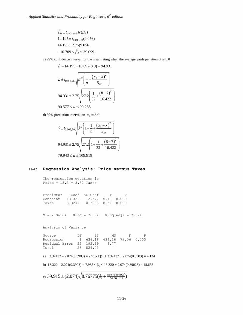
b) 99% confidence interval on 0
Applied Statistics and Probability for Engineers, 6th
edition
11-26
0 / 2, 2 0
0.005,30
0
ˆ ˆ( )
14.195 (9.056)
14.195 2.75(9.056)
ˆ10.709 39.099
nt se
t
c) 99% confidence interval for the mean rating when the average yards per attempt is 8.0
ˆ 14.195 10.092(8.0) 94.931
2
020.005,30
2
1ˆ ˆ
8 7194.931 2.75 27.2
32 16.422
90.577 99.285
xx
x xt
n S
d) 99% prediction interval on 0 8.0x
2
020.005,30
2
1ˆ ˆ 1
8 7194.931 2.75 27.2 1
32 16.422
79.943 109.919
xx
x xy t
n S
11-42 Regression Analysis: Price versus Taxes
The regression equation is
Price = 13.3 + 3.32 Taxes
Predictor Coef SE Coef T P
Constant 13.320 2.572 5.18 0.000
Taxes 3.3244 0.3903 8.52 0.000
S = 2.96104 R-Sq = 76.7% R-Sq(adj) = 75.7%
Analysis of Variance
Source DF SS MS F P
Regression 1 636.16 636.16 72.56 0.000
Residual Error 22 192.89 8.77
Total 23 829.05
a) 3.32437 – 2.074(0.3903) = 2.515 1 3.32437 + 2.074(0.3903) = 4.134
b) 13.320 – 2.074(0.3903) = 7.985 0 13.320 + 2.074(0.39028) = 18.655
c) )(76775.8)074.2(915.39 563139.57
)40492.60.8(
241
2
Applied Statistics and Probability for Engineers, 6th
edition
11-27
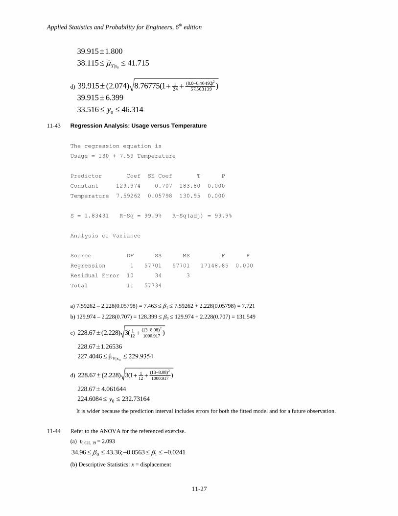
715.41ˆ115.38
800.1915.39
0|
xY
d) )1(76775.8)074.2(915.39 563139.57
)40492.60.8(
241
2
314.46516.33
399.6915.39
0
y
11-43 Regression Analysis: Usage versus Temperature
The regression equation is
Usage = 130 + 7.59 Temperature
Predictor Coef SE Coef T P
Constant 129.974 0.707 183.80 0.000
Temperature 7.59262 0.05798 130.95 0.000
S = 1.83431 R-Sq = 99.9% R-Sq(adj) = 99.9%
Analysis of Variance
Source DF SS MS F P
Regression 1 57701 57701 17148.85 0.000
Residual Error 10 34 3
Total 11 57734
a) 7.59262 – 2.228(0.05798) = 7.463 1 7.59262 + 2.228(0.05798) = 7.721
b) 129.974 – 2.228(0.707) = 128.399 0 129.974 + 2.228(0.707) = 131.549
c) 2(13 8.08)1
12 1000.917228.67 (2.228) 3( )
0Y|x
228.67 1.26536
ˆ227.4046 μ 229.9354
d) 2(13 8.08)1
12 1000.917228.67 (2.228) 3(1 )
0
228.67 4.061644
224.6084 232.73164y
It is wider because the prediction interval includes errors for both the fitted model and for a future observation.
11-44 Refer to the ANOVA for the referenced exercise.
(a) t0.025, 19 = 2.093
0 134.96 43.36; 0.0563 0.0241
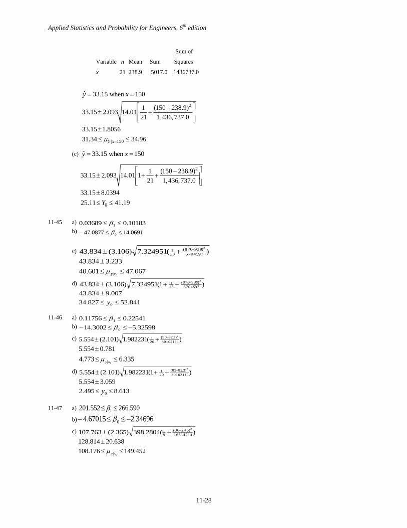
(b) Descriptive Statistics: x = displacement
Applied Statistics and Probability for Engineers, 6th
edition
11-28
Sum of
Variable n Mean Sum Squares
x 21 238.9 5017.0 1436737.0
2
| 150
ˆ 33.15 when 150
1 (150 238.9)33.15 2.093 14.01
21 1,436,737.0
33.15 1.8056
31.34 34.96Y x
y x
(c) ˆ 33.15 when 150y x
2
0
1 (150 238.9)33.15 2.093 14.01 1
21 1,436,737.0
33.15 8.0394
25.11 41.19Y
11-45 a) 10183.003689.0 1
b) 0691.140877.47 0
c) )(324951.7)106.3(834.43 97.67045
)939870(
131
2
067.47601.40
233.3834.43
0|
xy
d) )1(324951.7)106.3(834.4397.67045
)939870(
131
2
841.52827.34
007.9834.43
0
y
11-46 a) 22541.011756.0 1
b) 32598.53002.14 0
c) )(982231.1)101.2(554.52111.3010
)3.8290(
201
2
335.6773.4
781.0554.5
0|
xy
d) )1(982231.1)101.2(554.52111.3010
)3.8285(
201
2
613.8495.2
059.3554.5
0
y
11-47 a) 590.266552.201 1
b) 34696.267015.4 0
c) )(2804.398)365.2(763.1074214.1651
)5.2436(
91
2
452.149176.108
638.20814.128
0|
xy

Applied Statistics and Probability for Engineers, 6th
edition
11-29
11-48 a) 8239.263107.14 1
b) 12594.618501.5 0
c) )(8092.13)921.2(336.1701062.3
)806111.082.0(
181
2
896.19776.14
560.2336.17
0|
xy
d) )1(8092.13)921.2(336.1701062.3
)806111.082.0(
181
2
488.28184.6
152.11336.17
0
y
11-49 a) 1313.0885 196.0115
b) 017195.7176 18984.6824
c) 2(20 13.3375)1
20 1114.661812999.2 2.878 460992( )
0|
12999.2 585.64
12413.56 13584.84y x
d) 2(20 13.3375)1
20 1114.661812999.2 2.878 460992(1 )
0
12999.2 2039.93
10959.27 15039.14y
11-50 / 2, 2 0.005,5 4.032nt t
a) 99% confidence interval on 1
1 / 2, 2 1
0.001,5
1
ˆ ˆ( )
0.034 (0.026)
0.034 4.032(0.026)
ˆ0.1388 0.0708
nt se
t
b) 99% confidence interval on 0
0 / 2, 2 0
0.005,5
0
ˆ ˆ( )
55.63 (32.11)
55.63 4.032(32.11)
ˆ73.86 185.12
nt se
t
c) 99% confidence interval for the mean length when x = 1500:
ˆ 55.63 0.034(1500) 4.63
Applied Statistics and Probability for Engineers, 6th
edition
11-30
2
020.005,5
2
1ˆ ˆ
1500 1242.8614.63 4.032 77.33
7 117142.8
4.63 4.032(7.396)
25.19 34.45
xx
x xt
n S
d) 99% prediction interval when 0 1500x
2
020.005,5
2
0
1ˆ ˆ 1
1500 1242.8614.63 4.032 77.33 1
7 117142.8
4.63 4.032(11.49)
41.7 50.96
xx
x xy t
n S
y
It’s wider because it depends on both the error associated with the fitted model as well as that of the future
observation.
11-51 Refer to the computer output in the referenced exercise.
250.39,005.02,2/ tt n
a) 99% confidence interval for 1
2235.0ˆ1325.0
)014.0(250.3178.0
)014.0(178.0
)ˆ(ˆ
1
9,005.0
12,2/1
t
set n
b) 99% confidence interval on 0
196.1ˆ119.0
)1657.0(250.36578.0
)1657.0(6578.0
)ˆ(ˆ
0
9,005.0
02,2/0
t
set n
c) 95% confidence interval on when 100 x
Applied Statistics and Probability for Engineers, 6th
edition
11-31
635.2241.2
91.420
09.1010
11
1083.0262.2438.2
1ˆˆ
438.2)10(178.0658.0ˆ
0
0
0
|
2
2
02
9,025.0|
|
xy
xx
xy
xy
S
xx
nt
Section 11-7
11-52 8617.071.159
35.25330.2ˆ 22
1
2 YY
XX
S
SR
The model accounts for 86.17% of the variability in the data.
11-53 Refer to the Minitab output in the referenced exercise.
a) 2 0.672R
The model accounts for 67.2% of the variability in the data.
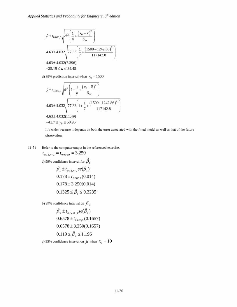
b) There is no major departure from the normality assumption in the following graph.
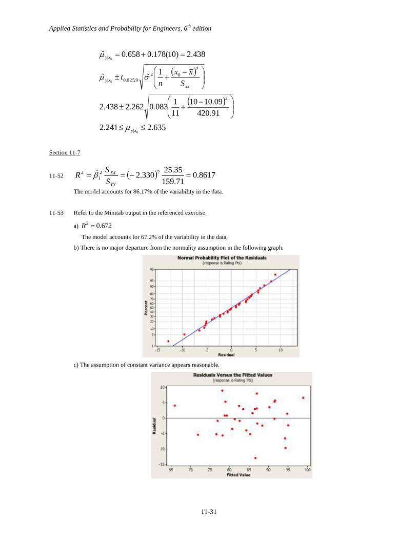
c) The assumption of constant variance appears reasonable.
Applied Statistics and Probability for Engineers, 6th
edition
11-32
11-54 Use the results from the referenced exercise to answer the following questions.
a) SalePrice Taxes Predicted Residuals
25.9 4.9176 29.6681073 -3.76810726
29.5 5.0208 30.0111824 -0.51118237
27.9 4.5429 28.4224654 -0.52246536
25.9 4.5573 28.4703363 -2.57033630
29.9 5.0597 30.1405004 -0.24050041
29.9 3.8910 26.2553078 3.64469225
30.9 5.8980 32.9273208 -2.02732082
28.9 5.6039 31.9496232 -3.04962324
35.9 5.8282 32.6952797 3.20472030
31.5 5.3003 30.9403441 0.55965587
31.0 6.2712 34.1679762 -3.16797616
30.9 5.9592 33.1307723 -2.23077234
30.0 5.0500 30.1082540 -0.10825401
36.9 8.2464 40.7342742 -3.83427422
41.9 6.6969 35.5831610 6.31683901
40.5 7.7841 39.1974174 1.30258260
43.9 9.0384 43.3671762 0.53282376
37.5 5.9894 33.2311683 4.26883165
37.9 7.5422 38.3932520 -0.49325200
44.5 8.7951 42.5583567 1.94164328
37.9 6.0831 33.5426619 4.35733807
38.9 8.3607 41.1142499 -2.21424985
36.9 8.1400 40.3805611 -3.48056112
45.8 9.1416 43.7102513 2.08974865
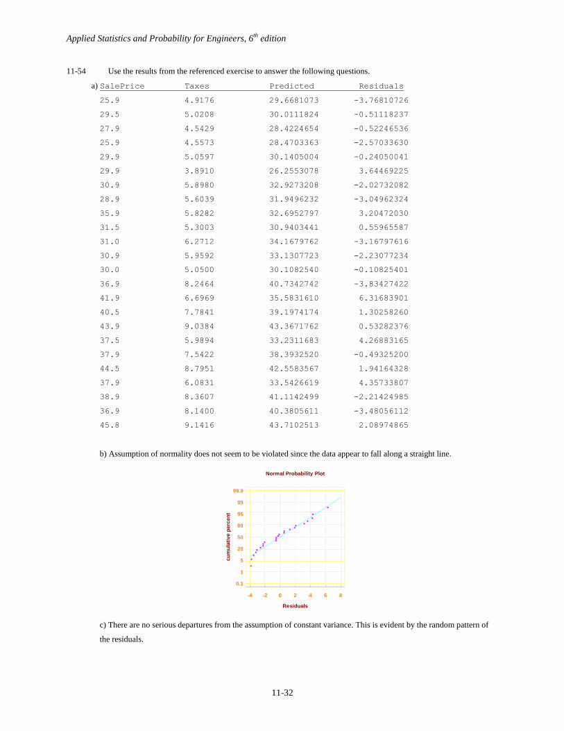
b) Assumption of normality does not seem to be violated since the data appear to fall along a straight line.
c) There are no serious departures from the assumption of constant variance. This is evident by the random pattern of
the residuals.
-4 -2 0 2 4 6 8
Residuals
Normal Probability Plot
0.1
1
5
20
50
80
95
99
99.9
cu
mu
lati
ve p
erc
en
t
Applied Statistics and Probability for Engineers, 6th
edition
11-33
d) 2 76.73%R ;
11-55 Use the results of the referenced exercise to answer the following questions
a) 2 99.986%;R The proportion of variability explained by the model.
b) Yes, normality seems to be satisfied because the data appear to fall along the straight line.
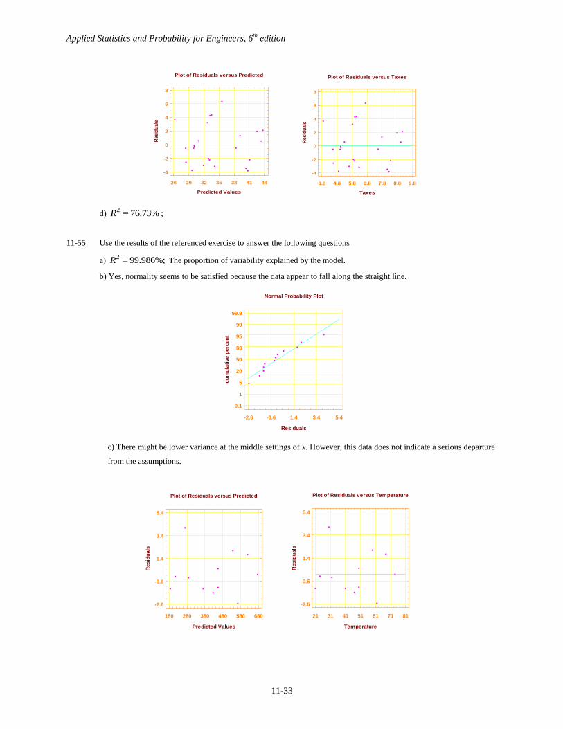
c) There might be lower variance at the middle settings of x. However, this data does not indicate a serious departure
from the assumptions.
26 29 32 35 38 41 44
Predicted Values
-4
-2
0
2
4
6
8
Resid
uals
Plot of Residuals versus Predicted
3.8 4.8 5.8 6.8 7.8 8.8 9.8
Taxes
-4
-2
0
2
4
6
8
Resid
uals
Plot of Residuals versus Taxes
-2.6 -0.6 1.4 3.4 5.4
Residuals
Normal Probability Plot
0.1
1
5
20
50
80
95
99
99.9
cu
mu
lati
ve p
erc
en
t
180 280 380 480 580 680
Predicted Values
-2.6
-0.6
1.4
3.4
5.4
Resid
uals
Plot of Residuals versus Predicted
21 31 41 51 61 71 81
Temperature
-2.6
-0.6
1.4
3.4
5.4
Res
idu
als
Plot of Residuals versus Temperature
Applied Statistics and Probability for Engineers, 6th
edition
11-34
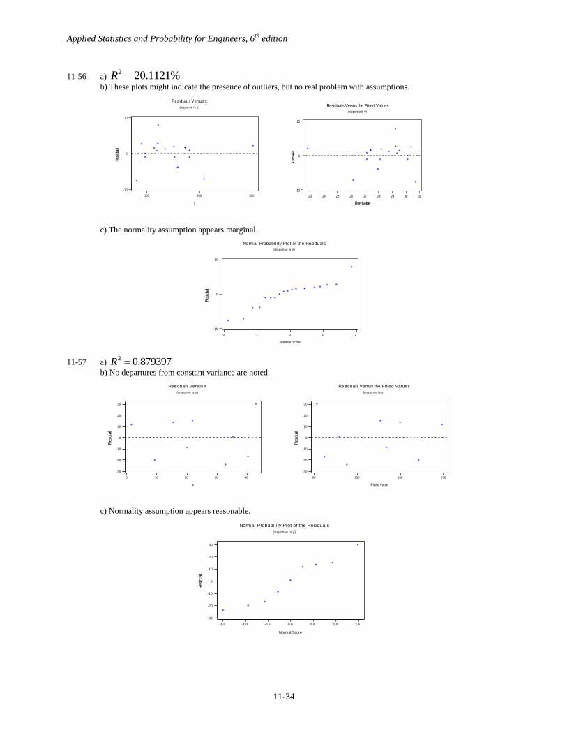
11-56 a) %1121.202 R
b) These plots might indicate the presence of outliers, but no real problem with assumptions.
c) The normality assumption appears marginal.
11-57 a) 879397.02 R
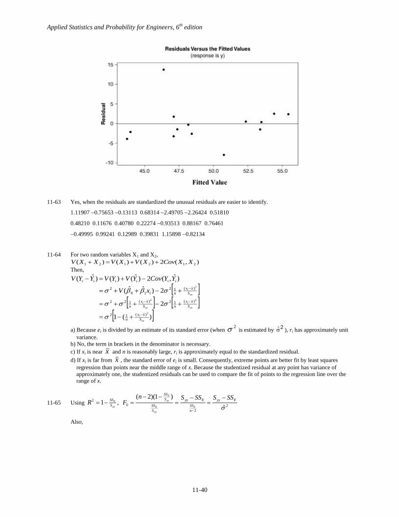
b) No departures from constant variance are noted.
c) Normality assumption appears reasonable.
300200100
10
0
-10
x
Res
idua
l
Residuals Versus x
(response is y)
3 1 3 0 2 9 2 8 2 7 2 6 2 5 2 4 2 3
1 0
0
- 1 0
F i t t e d V a l u e
R e s i d u a l
R e s i d u a l s V e r s u s t h e F i t t e d V a l u e s
( r e s p o n s e i s y )
210-1-2
10
0
-10
Normal Score
Res
idua
l
Normal Probability Plot of the Residuals
(response is y)
403020100
30
20
10
0
-10
-20
-30
x
Res
idua
l
Residuals Versus x
(response is y)
23018013080
30
20
10
0
-10
-20
-30
Fitted Value
Res
idua
l
Residuals Versus the Fitted Values
(response is y)
1.51.00.50.0-0.5-1.0-1.5
30
20
10
0
-10
-20
-30
Normal Score
Res
idua
l
Normal Probability Plot of the Residuals
(response is y)
Applied Statistics and Probability for Engineers, 6th
edition
11-35
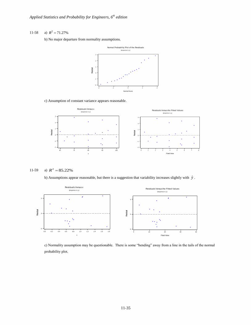
11-58 a) 2 71.27%R
b) No major departure from normality assumptions.
c) Assumption of constant variance appears reasonable.
11-59 a) %22.852 R
b) Assumptions appear reasonable, but there is a suggestion that variability increases slightly with y .
c) Normality assumption may be questionable. There is some “bending” away from a line in the tails of the normal
probability plot.
210-1-2
3
2
1
0
-1
-2
Normal ScoreR
esid
ual
Normal Probability Plot of the Residuals
(response is y)
10090807060
3
2
1
0
-1
-2
x
Res
idua
l
Residuals Versus x
(response is y)
876543210
3
2
1
0
-1
-2
Fitted Value
Res
idua
l
Residuals Versus the Fitted Values
(response is y)
1.81.61.41.21.00.80.60.40.20.0
5
0
-5
x
Res
idua
l
Residuals Versus x
(response is y)
403020100
5
0
-5
Fitted Value
Res
idua
l
Residuals Versus the Fitted Values
(response is y)

Applied Statistics and Probability for Engineers, 6th
edition
11-36
11-60 a)
The regression equation is
Compressive Strength = - 2150 + 185 Density
Predictor Coef SE Coef T P
Constant -2149.6 332.5 -6.46 0.000
Density 184.55 11.79 15.66 0.000
S = 339.219 R-Sq = 86.0% R-Sq(adj) = 85.6%
Analysis of Variance
Source DF SS MS F P
Regression 1 28209679 28209679 245.15 0.000
Residual Error 40 4602769 115069
Total 41 32812448
b) Because the P-value = 0.000 < = 0.01, the model is significant.
c) 2ˆ 115069
d) 2 28209679
1 0.8597 85.97%32812448
R E
T T
SS SSR
SS SS
The model accounts for 85.97% of the variability in the data.
e)
210-1-2
5
0
-5
Normal Score
Res
idua
l
Normal Probability Plot of the Residuals
(response is y)
Applied Statistics and Probability for Engineers, 6th
edition
11-37
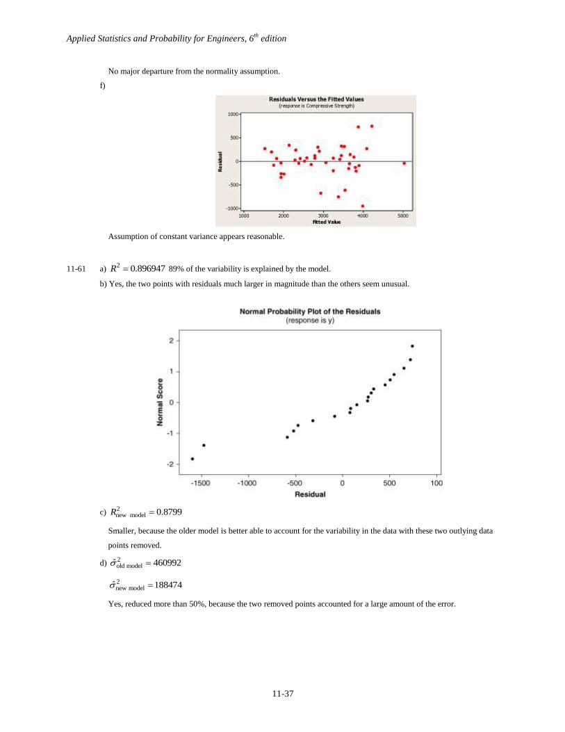
No major departure from the normality assumption.
f)
Assumption of constant variance appears reasonable.
11-61 a) 2 0.896947R 89% of the variability is explained by the model.
b) Yes, the two points with residuals much larger in magnitude than the others seem unusual.
c) 2new model 0.8799R
Smaller, because the older model is better able to account for the variability in the data with these two outlying data
points removed.
d) 2old modelˆ 460992
2new modelˆ 188474
Yes, reduced more than 50%, because the two removed points accounted for a large amount of the error.
Applied Statistics and Probability for Engineers, 6th
edition
11-38
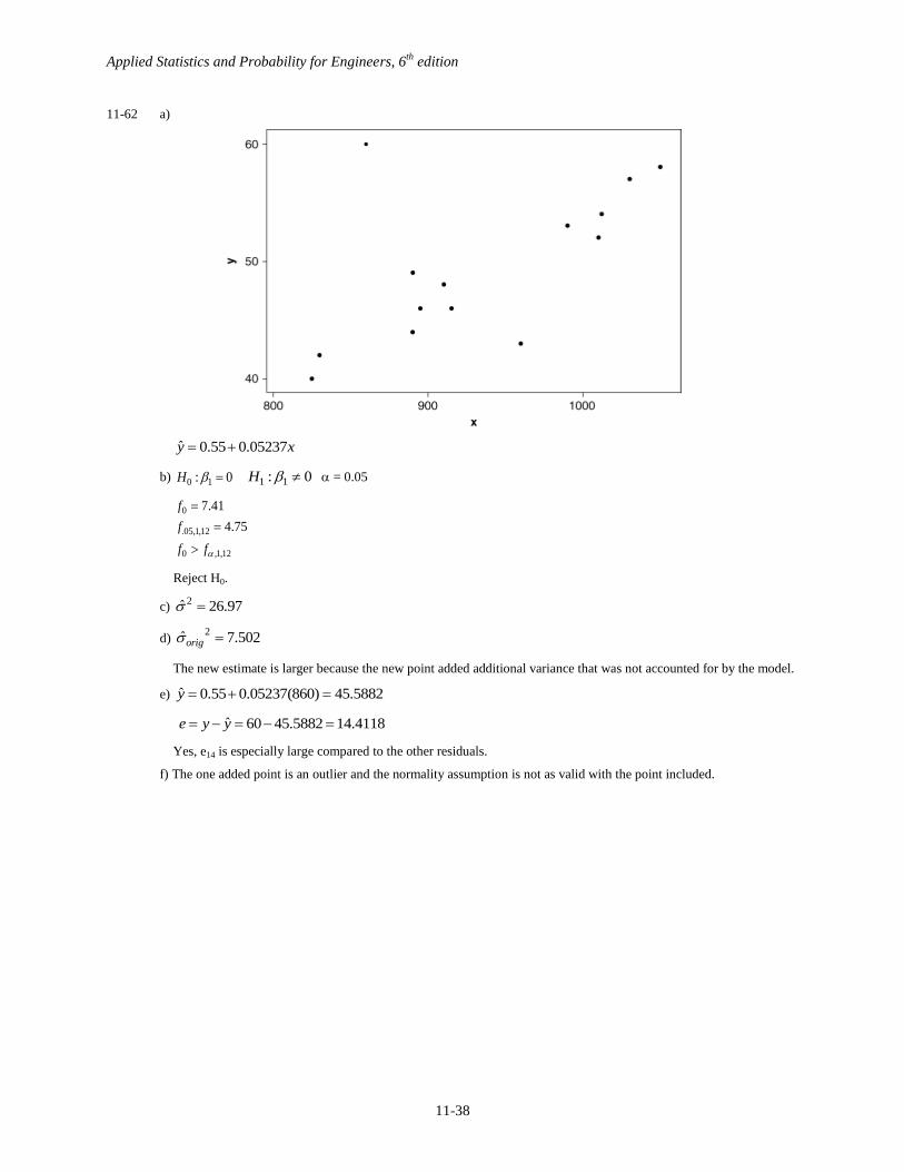
11-62 a)
ˆ 0.55 0.05237y x
b) 0 1: 0H 1 1: 0H = 0.05
0
.05,1,12
0 ,1,12
7.41
4.75
f
f
f f
Reject H0.
c) 2ˆ 26.97
d) 2ˆ 7.502orig
The new estimate is larger because the new point added additional variance that was not accounted for by the model.
e) ˆ 0.55 0.05237(860) 45.5882y
ˆ 60 45.5882 14.4118e y y
Yes, e14 is especially large compared to the other residuals.
f) The one added point is an outlier and the normality assumption is not as valid with the point included.

Applied Statistics and Probability for Engineers, 6th
edition
11-39
g) Constant variance assumption appears valid except for the added point.
x
Applied Statistics and Probability for Engineers, 6th
edition
11-40
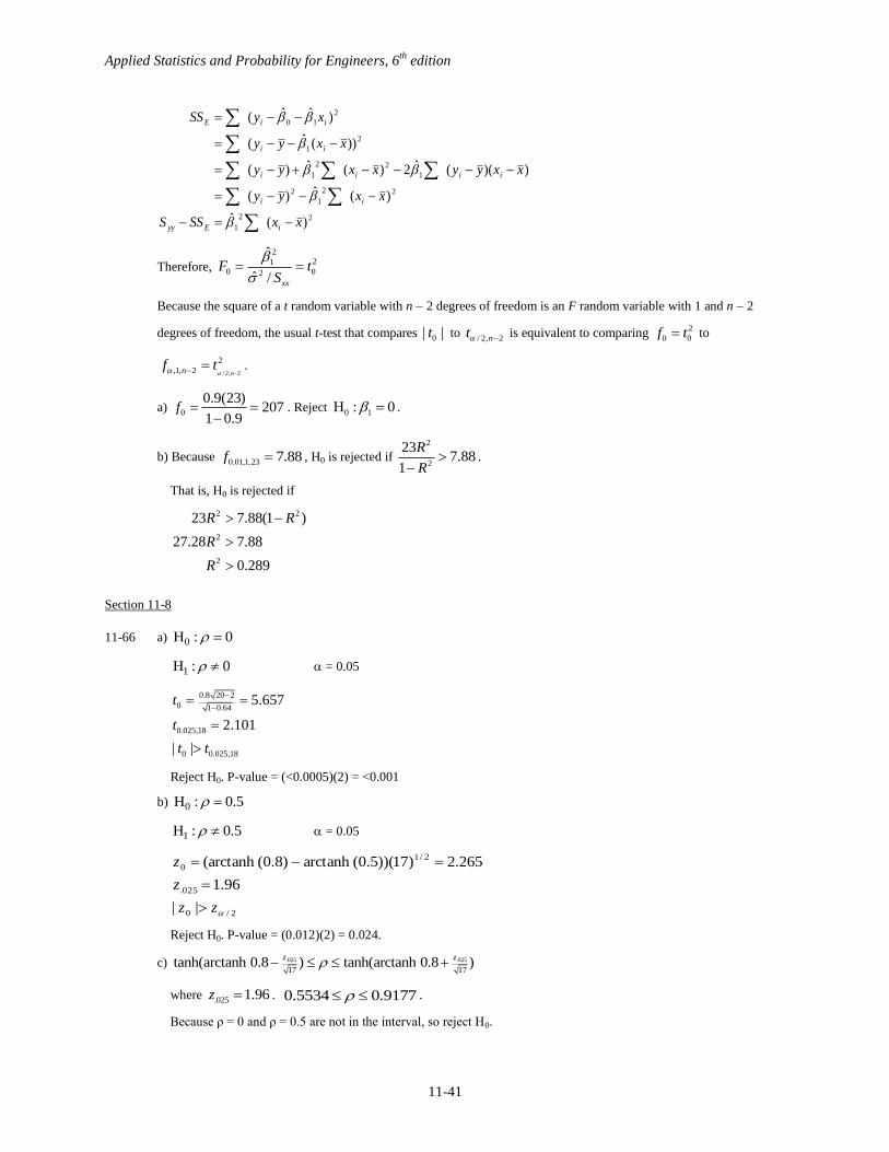
11-63 Yes, when the residuals are standardized the unusual residuals are easier to identify.
1.11907 0.75653 0.13113 0.68314 2.49705 2.26424 0.51810
0.48210 0.11676 0.40780 0.22274 0.93513 0.88167 0.76461
0.49995 0.99241 0.12989 0.39831 1.15898 0.82134
11-64 For two random variables X1 and X2,
),(2)()()( 212121 XXCovXVXVXXV
Then,
)(1
2
2)ˆˆ(
)ˆ,(2)ˆ()()ˆ(
2
22
2
)(12
)(12)(122
)(12
10
2
xx
i
xx
i
xx
i
xx
i
S
xx
n
S
xx
nS
xx
n
S
xx
ni
iiiiii
xV
YYCovYVYVYYV
a) Because ei is divided by an estimate of its standard error (when 2 is estimated by 2
), ri has approximately unit
variance.
b) No, the term in brackets in the denominator is necessary.
c) If xi is near x and n is reasonably large, ri is approximately equal to the standardized residual.
d) If xi is far from x , the standard error of ei is small. Consequently, extreme points are better fit by least squares
regression than points near the middle range of x. Because the studentized residual at any point has variance of
approximately one, the studentized residuals can be used to compare the fit of points to the regression line over the
range of x.
11-65 Using 2 1 ,E
yy
SS
SR 0 2
2
( 2)(1 )
ˆ
E
yy
E E
yy
SS
S yy E yy E
SS SS
S n
n S SS S SSF
Also,
Applied Statistics and Probability for Engineers, 6th
edition
11-41
22
1
22
1
2
1
22
1
2
1
2
10
)(ˆ
)(ˆ)(
))((ˆ2)(ˆ)(
))(ˆ(
)ˆˆ(
xxSSS
xxyy
xxyyxxyy
xxyy
xySS
iEyy
ii
iiii
ii
iiE
Therefore,
221
0 02
ˆ
ˆ / xx
F tS
Because the square of a t random variable with n 2 degrees of freedom is an F random variable with 1 and n 2
degrees of freedom, the usual t-test that compares 0| |t to / 2, 2nt
is equivalent to comparing 2
0 0f t to
/ 2, 2
2
,1, 2 nnf t .
a) 0
0.9(23)207
1 0.9f
. Reject 0 1H : 0 .
b) Because 0.01,1,23 7.88f , H0 is rejected if
2
2
237.88
1
R
R
.
That is, H0 is rejected if
2 2
2
2
23 7.88(1 )
27.28 7.88
0.289
R R
R
R
Section 11-8
11-66 a) 0H : 0
1H : 0 = 0.05
0.8 20 2
0 1 0.64
0.025,18
0 0.025,18
5.657
2.101
| |
t
t
t t
Reject H0. P-value = (<0.0005)(2) = <0.001
b) 0H : 0.5
1H : 0.5 = 0.05
2/0
025.
2/1
0
||
96.1
265.2)17)(0.5)(arctanh 0.8)((arctanh
zz
z
z
Reject H0. P-value = (0.012)(2) = 0.024.
c) .025 .025
17 17tanh(arctanh 0.8 ) tanh(arctanh 0.8 )
z z
where .025 1.96z . 9177.05534.0 .
Because ρ = 0 and ρ = 0.5 are not in the interval, so reject H0.
Applied Statistics and Probability for Engineers, 6th
edition
11-42
11-67 a) 0:0 H
0:1 H = 0.05
18,05.00
18,05.0
75.01
22075.0
0
734.1
81.42
tt
t
t
Reject H0. P-value < 0.0005
b) 1.0:0 H
1.0:1 H = 0.05
zz
z
z
0
05.
2/1
0
65.1
598.3)17)(0.1)(arctanh 0.75)((arctanh
Reject H0. P-value < 0.0002
c) )0.75nh tanh(arcta17
05.0z where 65.105. z
517.0
Because ρ = 0 and ρ = 0.1 are not in the interval, reject the null hypotheses from parts (a) and (b).
11-68 n = 30 r = 0.83
a) 0H : 0
1H : 0 = 0.05
2 2
2 0.83 28
01 1 (0.83)
.025,28
0 / 2,28
7.874
2.048
r n
rt
t
t t
Reject 0H . P-value = 0.
b) .025 .025
27 27tanh(arctanh 0.83 ) tanh(arctanh 0.83 )
z z
where .025 1.96z . 0.453 1.207 .
a) 0H : 0.8
1H : 0.8 = 0.05
1/ 2
0
.025
0 / 2
(arctanh 0.83 arctanh 0.8)(27) 0.4652
1.96
z
z
z z
Do not reject H0. P-value = (0.321)(2) = 0.642.
11-69 n = 50 r = 0.62
a) 0:0 H
0:1 H = 0.01
Applied Statistics and Probability for Engineers, 6th
edition
11-43
48,005.00
48,005.
)67.0(1
4867.0
1
2
0
682.2
253.622
tt
t
tr
nr
Reject H0. P-value 0
b) )+0.67nh tanh(arcta)-0.67nh tanh(arcta4747
005.005. zz
where 575.2005.0 z .
8294.04096.0
c) Yes.
11-70 a) r = 0.933203.
a) 0:0 H
0:1 H = 0.1
15,2/0
15,05.
)8709.0(1
15933203.0
1
2
0
753.1
06.102
tt
t
tr
nr
Reject H0
c) xy 498081.072538.0ˆ
0: 10 H
0: 11 H = 0.1
15,1,0
15,1,1.0
0
07.3
16.101
ff
f
f
Reject H0. Conclude that the model is significant at = 0.1. This test and the one in part b) are identical.
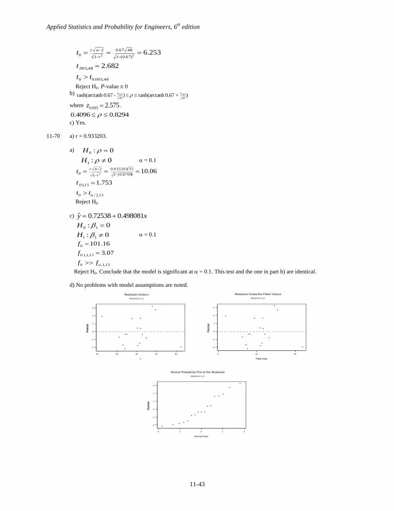
d) No problems with model assumptions are noted.
5040302010
3
2
1
0
-1
-2
x
Res
idua
l
Residuals Versus x
(response is y)
25155
3
2
1
0
-1
-2
Fitted Value
Res
idua
l
Residuals Versus the Fitted Values
(response is y)
210-1-2
3
2
1
0
-1
-2
Normal Score
Res
idua
l
Normal Probability Plot of the Residuals
(response is y)
Applied Statistics and Probability for Engineers, 6th
edition
11-44
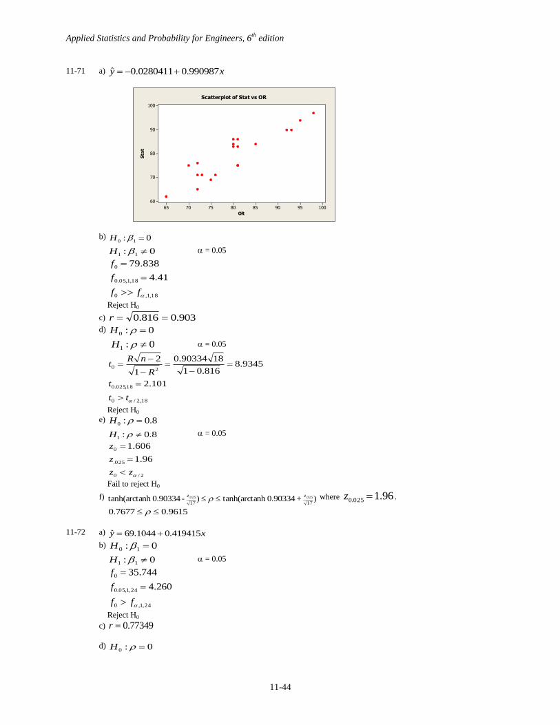
11-71 a) xy 990987.00280411.0ˆ
b) 0: 10 H
0: 11 H = 0.05
18,1,0
18,1,05.0
0
41.4
838.79
ff
f
f
Reject H0
c) 903.0816.0 r
d) 0:0 H
0:1 H = 0.05
18,2/0
18,025.0
20
101.2
9345.8816.01
1890334.0
1
2
tt
t
R
nRt
Reject H0
e) 8.0:0 H
8.0:1 H = 0.05
2/0
025.
0
96.1
606.1
zz
z
z
Fail to reject H0
f) )+0.90334nh tanh(arcta)-0.90334nh tanh(arcta1717
025.025. zz where 96.1025.0 z .
9615.07677.0
11-72 a) xy 419415.01044.69ˆ
b) 0: 10 H
0: 11 H = 0.05
24,1,0
24,1,05.0
0
260.4
744.35
ff
f
f
Reject H0
c) 77349.0r
d) 0:0 H
OR
Sta
t
10095908580757065
100
90
80
70
60
Scatterplot of Stat vs OR
Applied Statistics and Probability for Engineers, 6th
edition
11-45
0:1 H = 0.05
24,2/0
24,025.0
5983.01
2477349.0
0
064.2
9787.5
tt
t
t
Reject H0
e) 6.0:0 H
6.0:1 H = 0.05
2/0
025.
2/1
0
96.1
6105.1)23)(6.0arctanh 77349.0(arctanh
zz
z
z
Fail to reject H0
f) )+0.77349nh tanh(arcta)-0.77349nh tanh(arcta2323
025.025. zz where 96.1025.0 z
8932.05513.0
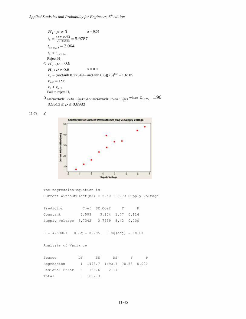
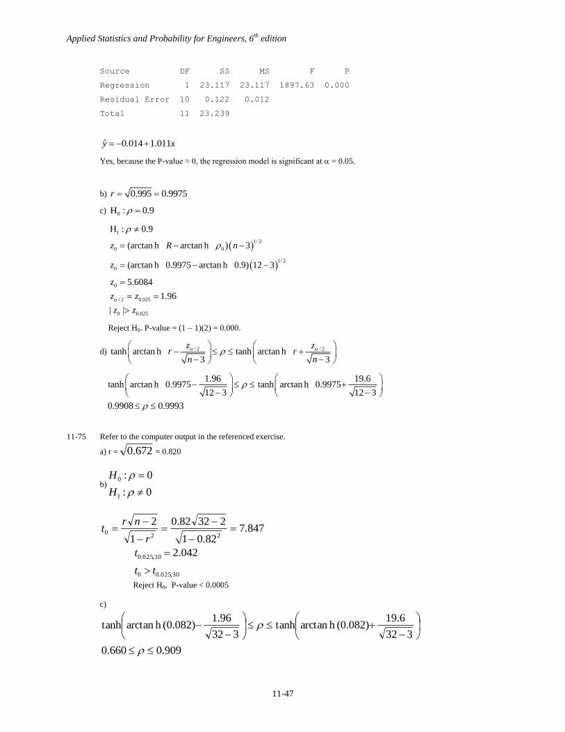
11-73 a)
The regression equation is
Current WithoutElect(mA) = 5.50 + 6.73 Supply Voltage
Predictor Coef SE Coef T P
Constant 5.503 3.104 1.77 0.114
Supply Voltage 6.7342 0.7999 8.42 0.000
S = 4.59061 R-Sq = 89.9% R-Sq(adj) = 88.6%
Analysis of Variance
Source DF SS MS F P
Regression 1 1493.7 1493.7 70.88 0.000
Residual Error 8 168.6 21.1
Total 9 1662.3
Applied Statistics and Probability for Engineers, 6th
edition
11-46
ˆ 5.50 6.73y x
Yes, because the P-value ≈ 0, the regression model is significant at = 0.05.
b) 0.899 0.948r
c) 0H : 0
1
02 2
0.025,8
0 0.025,8
H : 0
2 0.948 10 28.425
1 1 0.948
2.306
8.425 2.306
r nt
r
t
t t
Reject H0.
d) / 2 / 2tanh arctan h tanh arctan h3 3
z zr r
n n
1.96 19.6tanh arctan h 0.948 tanh arctan h 0.948
10 3 10 3
0.7898 0.9879
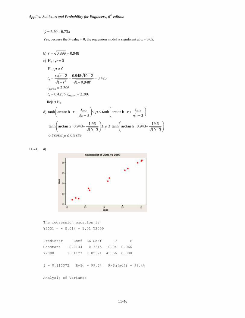
11-74 a)
The regression equation is
Y2001 = - 0.014 + 1.01 Y2000
Predictor Coef SE Coef T P
Constant -0.0144 0.3315 -0.04 0.966
Y2000 1.01127 0.02321 43.56 0.000
S = 0.110372 R-Sq = 99.5% R-Sq(adj) = 99.4%
Analysis of Variance
Applied Statistics and Probability for Engineers, 6th
edition
11-47
Source DF SS MS F P
Regression 1 23.117 23.117 1897.63 0.000
Residual Error 10 0.122 0.012
Total 11 23.239
ˆ 0.014 1.011y x
Yes, because the P-value ≈ 0, the regression model is significant at = 0.05.
b) 0.995 0.9975r
c) 0H : 0.9
1
1/ 2
0 0
1/ 2
0
0
/ 2 0.025
0 0.025
H : 0.9
(arctan h arctan h ) 3
(arctan h 0.9975 arctan h 0.9) 12 3
5.6084
1.96
| |
z R n
z
z
z z
z z
Reject H0. P-value = (1 1)(2) = 0.000.
d) / 2 / 2tanh arctan h tanh arctan h3 3
z zr r
n n
1.96 19.6tanh arctan h 0.9975 tanh arctan h 0.9975
12 3 12 3
0.9908 0.9993
11-75 Refer to the computer output in the referenced exercise.
a) r = 672.0 = 0.820
b)0:
0:
1
0
H
H
847.782.01
23282.0
1
2
220
r
nrt
30,025.00
30,025.0 042.2
tt
t
Reject H0, P-value < 0.0005
c)
909.0660.0
332
6.19(0.082)harctantanh
332
96.1)082.0(harctantanh
Applied Statistics and Probability for Engineers, 6th
edition
11-48
d)
025.00
025.02/
0
2/1
0
2/1
00
1
0
||
96.1
50.2
332)6.0harctan82.0h(arctan
3)harctanh(arctan
6.0:
6.0:
zz
zz
z
z
nRz
H
H
Reject H0, P-value = 2(0.00621) = 0.0124
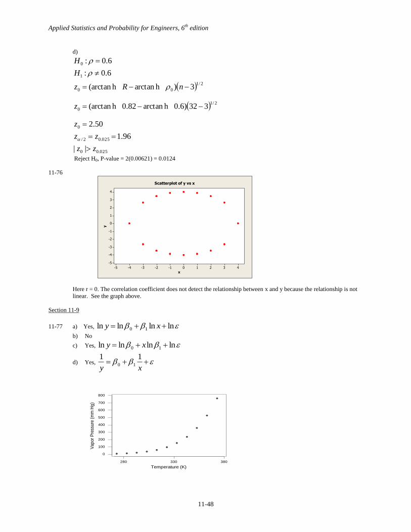
11-76
Here r = 0. The correlation coefficient does not detect the relationship between x and y because the relationship is not
linear. See the graph above.
Section 11-9
11-77 a) Yes, lnlnlnln 10 xy
b) No
c) Yes, lnlnlnln 10 xy
d) Yes, xy
1110
x
y
43210-1-2-3-4-5
4
3
2
1
0
-1
-2
-3
-4
-5
Scatterplot of y vs x
380330280
800
700
600
500
400
300
200
100
0
Temperature (K)
Vap
or P
ress
ure
(mm
Hg
)
Applied Statistics and Probability for Engineers, 6th
edition
11-49
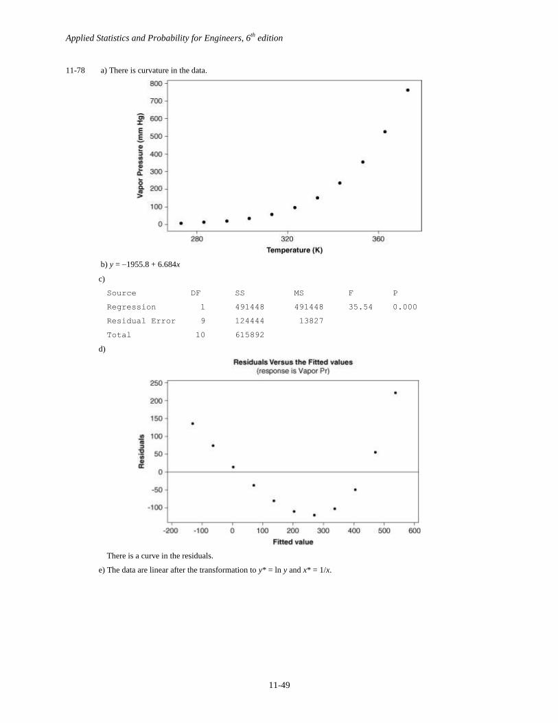
11-78 a) There is curvature in the data.
b) y = 1955.8 + 6.684x
c)
Source DF SS MS F P
Regression 1 491448 491448 35.54 0.000
Residual Error 9 124444 13827
Total 10 615892
d)
There is a curve in the residuals.
e) The data are linear after the transformation to y* = ln y and x* = 1/x.
Applied Statistics and Probability for Engineers, 6th
edition
11-50
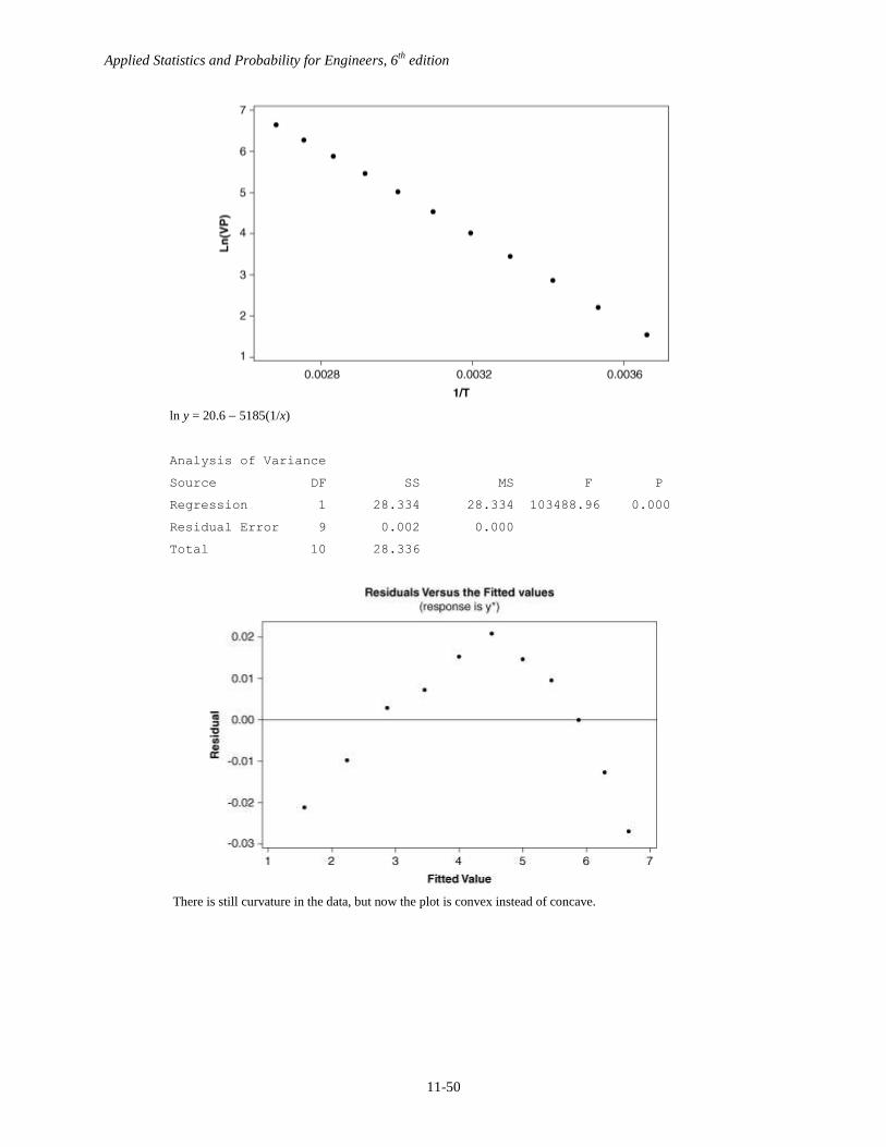
ln y = 20.6 5185(1/x)
Analysis of Variance
Source DF SS MS F P
Regression 1 28.334 28.334 103488.96 0.000
Residual Error 9 0.002 0.000
Total 10 28.336
There is still curvature in the data, but now the plot is convex instead of concave.
Applied Statistics and Probability for Engineers, 6th
edition
11-51
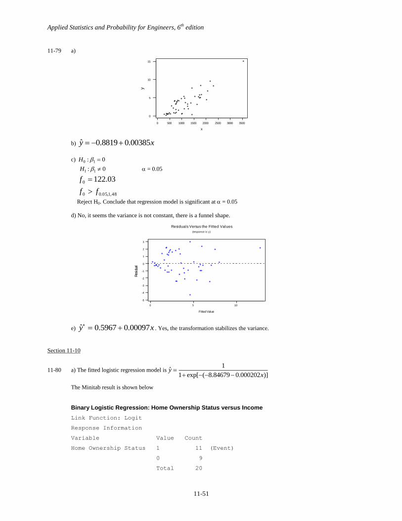
11-79 a)
b) xy 00385.08819.0ˆ
c) 0: 10 H
0: 11 H = 0.05
48,1,05.00
0 03.122
ff
f
Reject H0. Conclude that regression model is significant at = 0.05
d) No, it seems the variance is not constant, there is a funnel shape.
e) xy 00097.05967.0ˆ . Yes, the transformation stabilizes the variance.
Section 11-10
11-80 a) The fitted logistic regression model is1
ˆ1 exp[ ( 8.84679 0.000202 )]
yx
The Minitab result is shown below
Binary Logistic Regression: Home Ownership Status versus Income
Link Function: Logit
Response Information
Variable Value Count
Home Ownership Status 1 11 (Event)
0 9
Total 20
3500300025002000150010005000
15
10
5
0
x
y
1050
3
2
1
0
-1
-2
-3
-4
-5
Fitted Value
Res
idua
l
Residuals Versus the Fitted Values
(response is y)
Applied Statistics and Probability for Engineers, 6th
edition
11-52
Logistic Regression Table
Odds 95% CI
Predictor Coef SE Coef Z P Ratio Lower Upper
Constant -8.84679 4.44559 -1.99 0.047
Income 0.0002027 0.0001004 2.02 0.044 1.00 1.00 1.00
Log-Likelihood = -11.163
Test that all slopes are zero: G = 5.200, DF = 1, P-Value = 0.023
b) The P-value for the test of the coefficient of income is 0.044 < = 0.05. Therefore, income has a significant effect
on home ownership status.
c) The odds ratio is changed by the factor exp(1) = exp(0.0002027) = 1.000202 for every unit increase in income.
More realistically, if income changes by $1000, the odds ratio is changed by the factor exp(10001) = exp(0.2027) =
1.225.
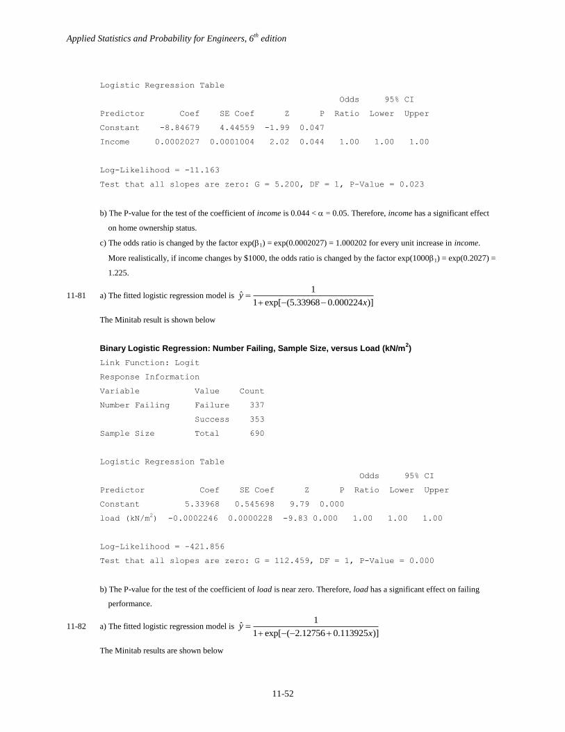
11-81 a) The fitted logistic regression model is 1
ˆ1 exp[ (5.33968 0.000224 )]
yx
The Minitab result is shown below
Binary Logistic Regression: Number Failing, Sample Size, versus Load (kN/m2)
Link Function: Logit
Response Information
Variable Value Count
Number Failing Failure 337
Success 353
Sample Size Total 690
Logistic Regression Table
Odds 95% CI
Predictor Coef SE Coef Z P Ratio Lower Upper
Constant 5.33968 0.545698 9.79 0.000
load (kN/m2) -0.0002246 0.0000228 -9.83 0.000 1.00 1.00 1.00
Log-Likelihood = -421.856
Test that all slopes are zero: G = 112.459, DF = 1, P-Value = 0.000
b) The P-value for the test of the coefficient of load is near zero. Therefore, load has a significant effect on failing
performance.
11-82 a) The fitted logistic regression model is 1
ˆ1 exp[ ( 2.12756 0.113925 )]
yx
The Minitab results are shown below
Applied Statistics and Probability for Engineers, 6th
edition
11-53
Binary Logistic Regression: Number Redee, Sample size, versus Discount, x
Link Function: Logit
Response Information
Variable Value Count
Number Redeemed Success 2693
Failure 3907
Sample Size Total 6600
Logistic Regression Table
Odds 95% CI
Predictor Coef SE Coef Z P Ratio Lower Upper
Constant -2.12756 0.0746903 -28.49 0.000
Discount, x 0.113925 0.0044196 25.78 0.000 1.12 1.11 1.13
Log-Likelihood = -4091.801
Test that all slopes are zero: G = 741.361, DF = 1, P-Value = 0.000
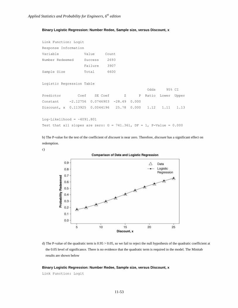
b) The P-value for the test of the coefficient of discount is near zero. Therefore, discount has a significant effect on
redemption.
c)
d) The P-value of the quadratic term is 0.95 > 0.05, so we fail to reject the null hypothesis of the quadratic coefficient at
the 0.05 level of significance. There is no evidence that the quadratic term is required in the model. The Minitab
results are shown below
Binary Logistic Regression: Number Redee, Sample size, versus Discount, x
Link Function: Logit
Applied Statistics and Probability for Engineers, 6th
edition
11-54
Response Information
Variable Value Count
Number Redeemed Event 2693
Non-event 3907
Sample Size Total 6600
Logistic Regression Table
95%
Odds CI
Predictor Coef SE Coef Z P Ratio Lower
Constant -2.34947 0.174523 -13.46 0.000
Discount, x 0.148003 0.0245118 6.04 0.000 1.16 1.11
Discount, x* Discount, x -0.0011084 0.0007827 -1.42 0.157 1.00 1.00
Predictor Upper
Constant
Discount, x 1.22
Discount, x*Discount, x 1.00
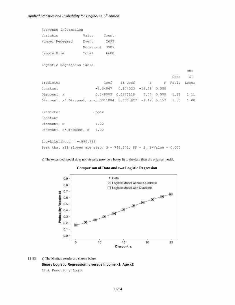
Log-Likelihood = -4090.796
Test that all slopes are zero: G = 743.372, DF = 2, P-Value = 0.000
e) The expanded model does not visually provide a better fit to the data than the original model.
11-83 a) The Minitab results are shown below
Binary Logistic Regression: y versus Income x1, Age x2
Link Function: Logit
Comparison of Data and two Logistic Regression
Applied Statistics and Probability for Engineers, 6th
edition
11-55
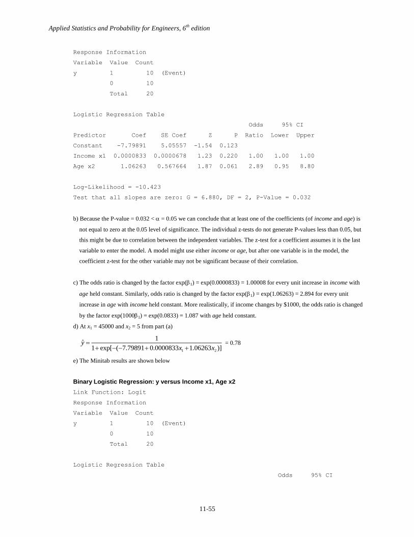
Response Information
Variable Value Count
y 1 10 (Event)
0 10
Total 20
Logistic Regression Table
Odds 95% CI
Predictor Coef SE Coef Z P Ratio Lower Upper
Constant -7.79891 5.05557 -1.54 0.123
Income x1 0.0000833 0.0000678 1.23 0.220 1.00 1.00 1.00
Age x2 1.06263 0.567664 1.87 0.061 2.89 0.95 8.80
Log-Likelihood = -10.423
Test that all slopes are zero: G = 6.880, DF = 2, P-Value = 0.032
b) Because the P-value = 0.032 < = 0.05 we can conclude that at least one of the coefficients (of income and age) is
not equal to zero at the 0.05 level of significance. The individual z-tests do not generate P-values less than 0.05, but
this might be due to correlation between the independent variables. The z-test for a coefficient assumes it is the last
variable to enter the model. A model might use either income or age, but after one variable is in the model, the
coefficient z-test for the other variable may not be significant because of their correlation.
c) The odds ratio is changed by the factor exp(1) = exp(0.0000833) = 1.00008 for every unit increase in income with
age held constant. Similarly, odds ratio is changed by the factor exp(1) = exp(1.06263) = 2.894 for every unit
increase in age with income held constant. More realistically, if income changes by $1000, the odds ratio is changed
by the factor exp(10001) = exp(0.0833) = 1.087 with age held constant.
d) At x1 = 45000 and x2 = 5 from part (a)
1 2
1ˆ
1 exp[ ( 7.79891 0.0000833 1.06263 )]y
x x
= 0.78
e) The Minitab results are shown below
Binary Logistic Regression: y versus Income x1, Age x2
Link Function: Logit
Response Information
Variable Value Count
y 1 10 (Event)
0 10
Total 20
Logistic Regression Table
Odds 95% CI
Applied Statistics and Probability for Engineers, 6th
edition
11-56
Predictor Coef SE Coef Z P Ratio Lower Upper
Constant -0.494471 6.64311 -0.07 0.941
Income x1 -0.0001314 0.0001411 -0.93 0.352 1.00 1.00 1.00
Age x2 -2.39447 2.07134 -1.16 0.248 0.09 0.00 5.29
Income x1*Age x2 0.0001017 0.0000626 1.62 0.104 1.00 1.00 1.00
Log-Likelihood = -8.112
Test that all slopes are zero: G = 11.503, DF = 3, P-Value = 0.009
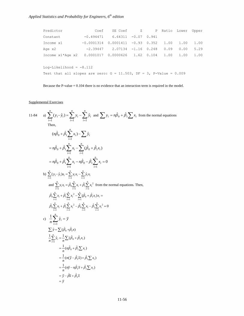
Because the P-value = 0.104 there is no evidence that an interaction term is required in the model.
Supplemental Exercises
11-84 a)
n
i
i
n
i
i
n
i
ii yyyy
111
ˆ)ˆ( and ii xny 10ˆˆ from the normal equations
Then,
0ˆˆˆˆ
)ˆˆ(ˆˆ
ˆ)ˆˆ(
1
10
1
10
1
10
1
10
1
10
n
i
i
n
i
i
n
i
i
n
i
i
i
n
i
i
xnxn
xxn
yxn
b) i
n
iii
n
iii
n
iii xyxyxyy
111
ˆ)ˆ(
and
n
ii
n
iii
n
ii xxxy
1
21
10
1
ˆˆ from the normal equations. Then,
0ˆˆˆˆ
)ˆˆ(ˆˆ
1
21
10
1
21
10
1011
21
10
n
ii
n
ii
n
ii
n
ii
ii
n
i
n
ii
n
ii
xxxx
xxxx
c) yyn
n
i
i 1
ˆ1
)ˆˆ(ˆ10 xy
y
xxy
xxnynn
xxynn
xnn
xn
yn
i
i
i
i
n
ii
1
11
11
10
101
ˆˆ
)ˆˆ(1
)ˆ)ˆ((1
)ˆˆ(1
)ˆˆ(1
ˆ1
Applied Statistics and Probability for Engineers, 6th
edition
11-57
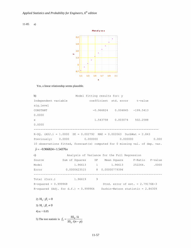
11-85 a)
Yes, a linear relationship seems plausible.
b) Model fitting results for: y
Independent variable coefficient std. error t-value
sig.level
CONSTANT -0.966824 0.004845 -199.5413
0.0000
x 1.543758 0.003074 502.2588
0.0000
--------------------------------------------------------------------------
R-SQ. (ADJ.) = 1.0000 SE = 0.002792 MAE = 0.002063 DurbWat = 2.843
Previously: 0.0000 0.000000 0.000000 0.000
10 observations fitted, forecast(s) computed for 0 missing val. of dep. var.
ˆ 0.966824 1.54376y x
c) Analysis of Variance for the Full Regression
Source Sum of Squares DF Mean Square F-Ratio P-value
Model 1.96613 1 1.96613 252264. .0000
Error 0.0000623515 8 0.00000779394
----------------------------------------------------------------------------
Total (Corr.) 1.96619 9
R-squared = 0.999968 Stnd. error of est. = 2.79176E-3
R-squared (Adj. for d.f.) = 0.999964 Durbin-Watson statistic = 2.84309
2) 0 1H : 0
3) 1 1H : 0
4) = 0.05
5) The test statistic is 0
/
/( )
R
E
SS kf
SS n p
1.1 1.3 1.5 1.7 1.9 2.1
x
0.7
1
1.3
1.6
1.9
2.2
y
Plot of y vs x
Applied Statistics and Probability for Engineers, 6th
edition
11-58
6) Reject H0 if f0 > f,1,8 where f0.01,1,8 = 11.26
7) Using the results from the ANOVA table
0
1.96613/1252263.9
0.0000623515/8f
8) Because 252264 > 11.26 reject H0 and conclude that the regression model is significant at = 0.05.
P-value ≈ 0
d) 99 percent confidence intervals for coefficient estimates
---------------------------------------------------------------------------
Estimate Standard error Lower Limit Upper Limit
CONSTANT -0.96682 0.00485 -0.97800 -0.95565
x 1.54376 0.00307 1.53667 1.55085
---------------------------------------------------------------------------
11.53667 1.55085
e) 2) 0 0H : 0
3) 1 0H : 0
4) = 0.01
5) The test statistic is 00
0
ˆ
ˆ( )t
se
6) Reject H0 if t0 < t/2,n-2 where t0.005,8 = 3.355 or t0 > t0.005,8 = 3.355
7) Using the results from the table above
0
0.96682199.34
0.00485t
8) Since 199.34 < 3.355 reject H0 and conclude the intercept is significant at = 0.05.
11-86 a) ˆ 93.55 15.57y x
b) 0 1H : 0
1 1H : 0
= 0.05
0
.05,1,14
0 0.05,1,14
12.872
4.60
f
f
f f
Reject H0. Conclude that 1 0 at = 0.05.
c) 1(9.689 21.445)
d) 0(79.333 107.767)
e) ˆ 93.55 15.57(2.5) 132.475y
Applied Statistics and Probability for Engineers, 6th
edition
11-59
2
0
(2.5 2.325)1
16 7.017
| 2.5
132.475 2.145 136.9
132.475 6.49
ˆ125.99 138.97Y x
11-87 xy 5086.02166.1ˆ where yy /1
. No, the model does not seem reasonable.
The residual plots indicate a possible outlier.
11-88 ˆ 4.5067 2.21517y x , r = 0.992, R2 = 98.43%
The model appears to be an excellent fit. The R2 is large and both regression coefficients are significant. No, the
existence of a strong correlation does not imply a cause and effect relationship.
11-89 xy 7916.0ˆ
Even though y should be zero when x is zero, because the regressor variable does not usually assume values near zero, a
model with an intercept fits this data better. Without an intercept, the residuals plots are not satisfactory.
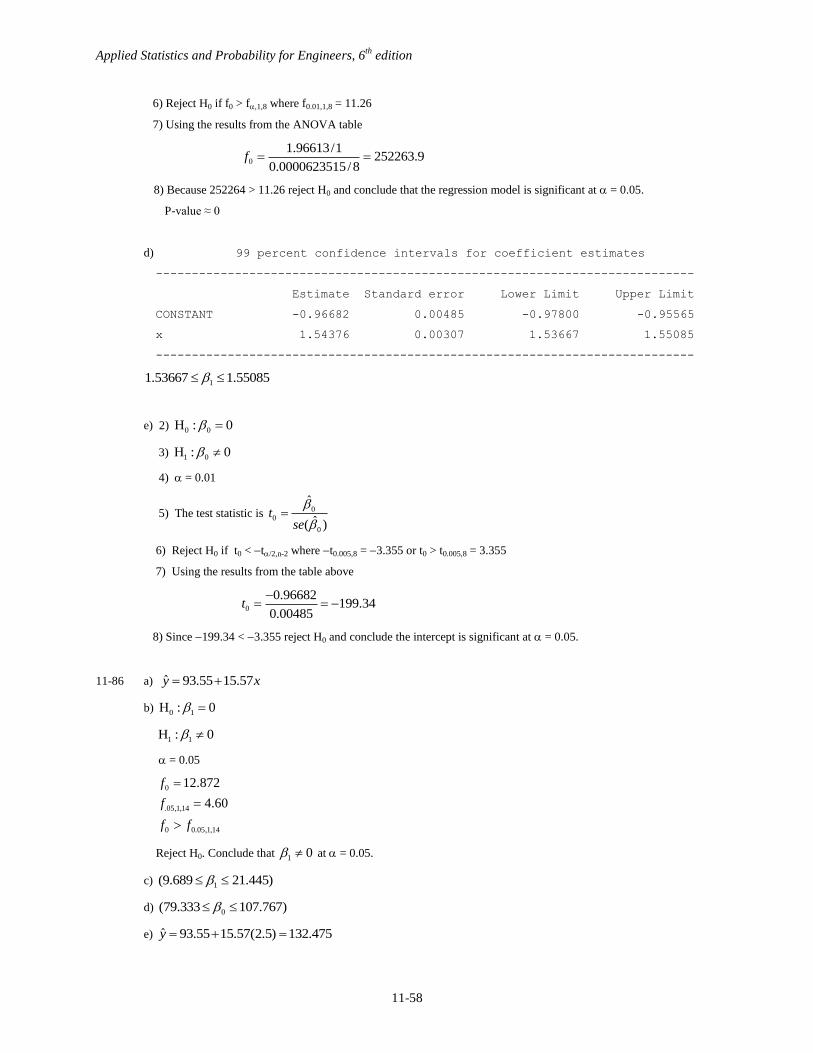
11-90 a)
b) The regression equation is
xy 296.15193ˆ
Analysis of Variance
Source DF SS MS F P
Regression 1 1492.6 1492.6 2.64 0.127
Residual Error 14 7926.8 566.2
Total 15 9419.4
Fail to reject Ho. We do not have evidence of a relationship. Therefore, there is not sufficient evidence to conclude that
the seasonal meteorological index (x) is a reliable predictor of the number of days that the ozone level exceeds 0.20
ppm (y).
c) 99% CI on 1
)5194.1,1402.3(
)2697.0(005.33298.2
)2697.0(3298.2
)ˆ(ˆ
12,005.
12,2/1
t
set n
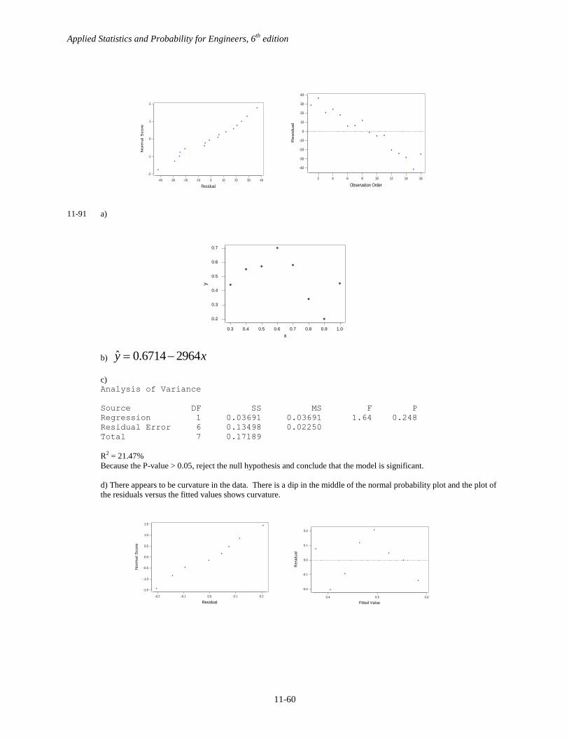
d) The normality plot of the residuals is satisfactory. However, the plot of residuals versus run order exhibits a strong
downward trend. This could indicate that there is another variable should be included in the model and it is one that
changes with time.
181716
110
100
90
80
70
60
50
40
30
index
days
Applied Statistics and Probability for Engineers, 6th
edition
11-60
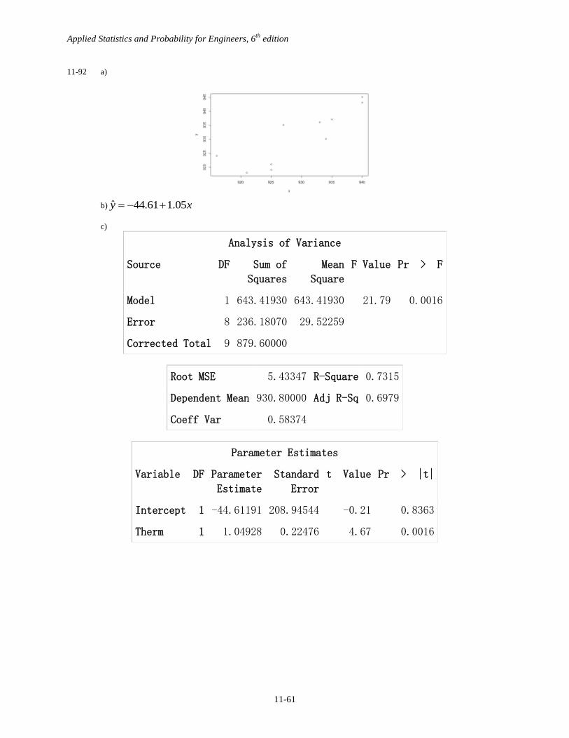
11-91 a)
b) xy 29646714.0ˆ
c) Analysis of Variance
Source DF SS MS F P
Regression 1 0.03691 0.03691 1.64 0.248
Residual Error 6 0.13498 0.02250
Total 7 0.17189
R2 = 21.47%
Because the P-value > 0.05, reject the null hypothesis and conclude that the model is significant.
d) There appears to be curvature in the data. There is a dip in the middle of the normal probability plot and the plot of
the residuals versus the fitted values shows curvature.
403020100-10-20-30-40
2
1
0
-1
-2
No
rma
l S
co
re
Residual
161412108642
40
30
20
10
0
-10
-20
-30
-40
Observation Order
Re
sid
ua
l
1.00.90.80.70.60.50.40.3
0.7
0.6
0.5
0.4
0.3
0.2
x
y
0.20.10.0-0.1-0.2
1.5
1.0
0.5
0.0
-0.5
-1.0
-1.5
No
rma
l S
co
re
Residual
0.4 0.5 0.6
-0.2
-0.1
0.0
0.1
0.2
Fitted Value
Re
sid
ua
l
Applied Statistics and Probability for Engineers, 6th
edition
11-61
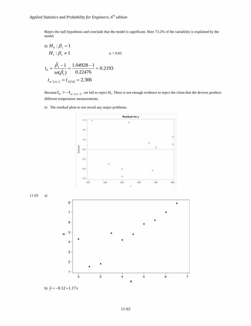
11-92 a)
b) xy 05.161.44ˆ
c)
Analysis of Variance
Source DF Sum of
Squares
Mean
Square
F Value Pr > F
Model 1 643.41930 643.41930 21.79 0.0016
Error 8 236.18070 29.52259
Corrected Total 9 879.60000
Root MSE 5.43347 R-Square 0.7315
Dependent Mean 930.80000 Adj R-Sq 0.6979
Coeff Var 0.58374
Parameter Estimates
Variable DF Parameter
Estimate
Standard
Error
t Value Pr > |t|
Intercept 1 -44.61191 208.94544 -0.21 0.8363
Therm 1 1.04928 0.22476 4.67 0.0016
Applied Statistics and Probability for Engineers, 6th
edition
11-62
Reject the null hypothesis and conclude that the model is significant. Here 73.2% of the variability is explained by the
model.
d) 1: 10 H
1: 11 H = 0.05
2193.022476.0
11.04928
)ˆ(
1ˆ
1
10
set
306.28,025.2,2/ tt na
Because 2,2/0 natt , we fail to reject Ho. There is not enough evidence to reject the claim that the devices produce
different temperature measurements.
e) The residual plots to not reveal any major problems.
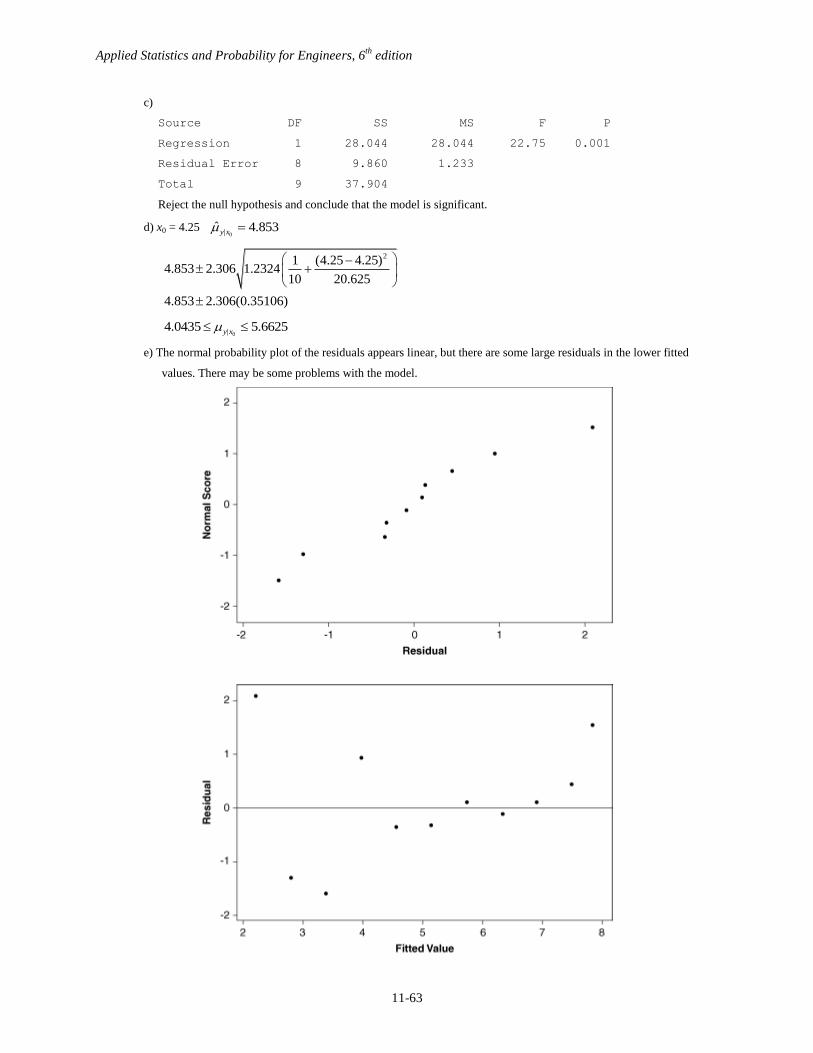
11-93 a)
b) ˆ 0.12 1.17y x
Applied Statistics and Probability for Engineers, 6th
edition
11-63
c)
Source DF SS MS F P
Regression 1 28.044 28.044 22.75 0.001
Residual Error 8 9.860 1.233
Total 9 37.904
Reject the null hypothesis and conclude that the model is significant.
d) x0 = 4.25 0|
ˆ 4.853y x
21 (4.25 4.25)4.853 2.306 1.2324
10 20.625
4.853 2.306(0.35106)
0|4.0435 5.6625y x
e) The normal probability plot of the residuals appears linear, but there are some large residuals in the lower fitted
values. There may be some problems with the model.
Applied Statistics and Probability for Engineers, 6th
edition
11-64
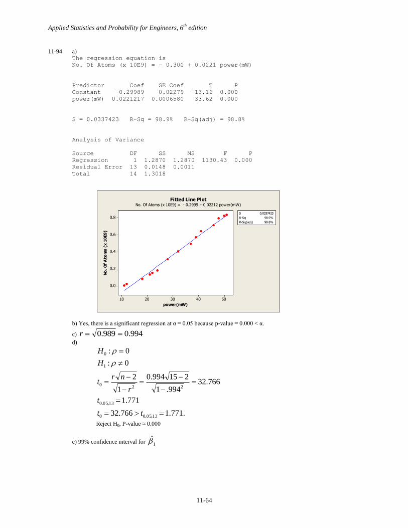
11-94 a) The regression equation is
No. Of Atoms (x 10E9) = - 0.300 + 0.0221 power(mW)
Predictor Coef SE Coef T P
Constant -0.29989 0.02279 -13.16 0.000
power(mW) 0.0221217 0.0006580 33.62 0.000
S = 0.0337423 R-Sq = 98.9% R-Sq(adj) = 98.8%
Analysis of Variance
Source DF SS MS F P
Regression 1 1.2870 1.2870 1130.43 0.000
Residual Error 13 0.0148 0.0011
Total 14 1.3018
b) Yes, there is a significant regression at α = 0.05 because p-value = 0.000 < α.
c) 994.0989.0 r
d)
.771.1766.32
771.1
766.32994.1
215994.0
1
2
0:
0:
13,05.00
13,05.0
220
1
0
tt
t
r
nrt
H
H
Reject H0, P-value ≈ 0.000
e) 99% confidence interval for 1
power(mW)
No
. O
f A
tom
s (
x 1
0E9
)
5040302010
0.8
0.6
0.4
0.2
0.0
S 0.0337423
R-Sq 98.9%
R-Sq(adj) 98.8%
Fitted Line PlotNo. Of Atoms (x 10E9) = - 0.2999 + 0.02212 power(mW)
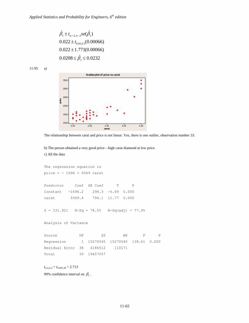
Applied Statistics and Probability for Engineers, 6th
edition
11-65
0232.0ˆ0208.0
)00066.0(771.1022.0
)00066.0(022.0
)ˆ(ˆ
1
13,05.0
12,2/1
t
set n
11-95 a)
The relationship between carat and price is not linear. Yes, there is one outlier, observation number 33.
b) The person obtained a very good price—high carat diamond at low price.
c) All the data
The regression equation is
price = - 1696 + 9349 carat
Predictor Coef SE Coef T P
Constant -1696.2 298.3 -5.69 0.000
carat 9349.4 794.1 11.77 0.000
S = 331.921 R-Sq = 78.5% R-Sq(adj) = 77.9%
Analysis of Variance
Source DF SS MS F P
Regression 1 15270545 15270545 138.61 0.000
Residual Error 38 4186512 110171
Total 39 19457057
t/2,n-2 = t0.005,38 = 2.713
99% confidence interval on 1 .
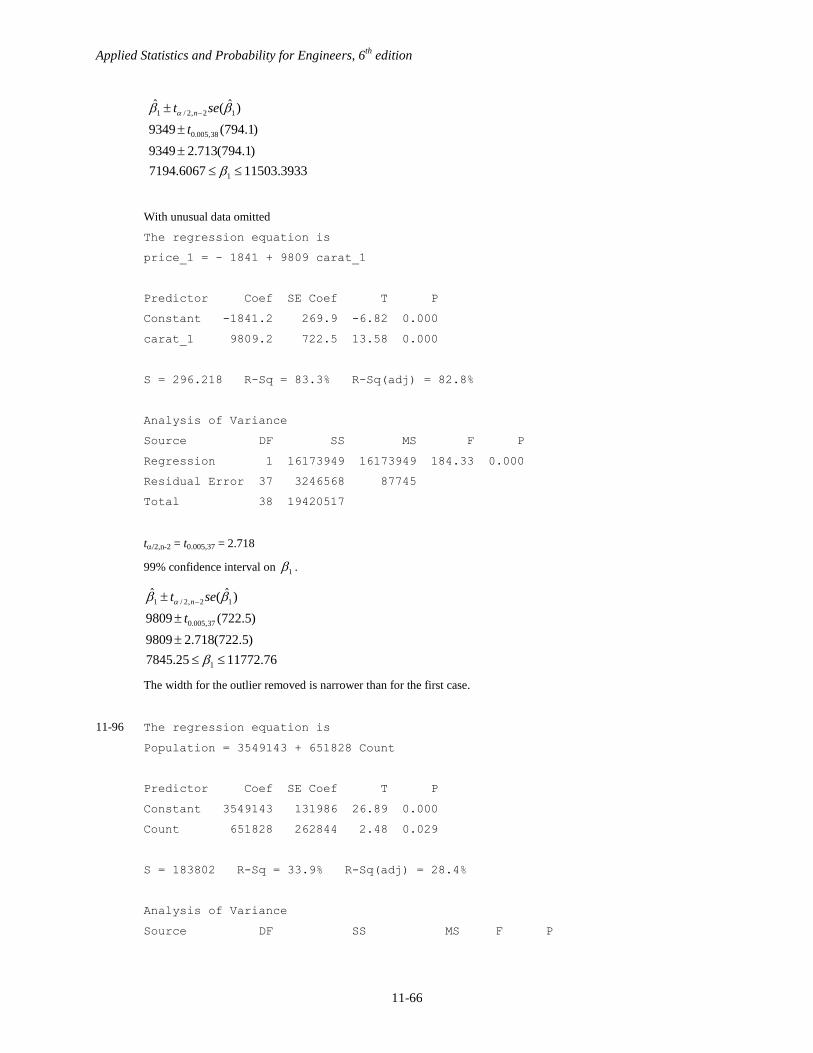
Applied Statistics and Probability for Engineers, 6th
edition
11-66
1 / 2, 2 1
0.005,38
1
ˆ ˆ( )
9349 (794.1)
9349 2.713(794.1)
7194.6067 11503.3933
nt se
t
With unusual data omitted
The regression equation is
price_1 = - 1841 + 9809 carat_1
Predictor Coef SE Coef T P
Constant -1841.2 269.9 -6.82 0.000
carat_1 9809.2 722.5 13.58 0.000
S = 296.218 R-Sq = 83.3% R-Sq(adj) = 82.8%
Analysis of Variance
Source DF SS MS F P
Regression 1 16173949 16173949 184.33 0.000
Residual Error 37 3246568 87745
Total 38 19420517
t/2,n-2 = t0.005,37 = 2.718
99% confidence interval on 1 .
1 / 2, 2 1
0.005,37
1
ˆ ˆ( )
9809 (722.5)
9809 2.718(722.5)
7845.25 11772.76
nt se
t
The width for the outlier removed is narrower than for the first case.
11-96 The regression equation is
Population = 3549143 + 651828 Count
Predictor Coef SE Coef T P
Constant 3549143 131986 26.89 0.000
Count 651828 262844 2.48 0.029
S = 183802 R-Sq = 33.9% R-Sq(adj) = 28.4%
Analysis of Variance
Source DF SS MS F P
Applied Statistics and Probability for Engineers, 6th
edition
11-67
Regression 1 2.07763E+11 2.07763E+11 6.15 0.029
Residual Error 12 4.05398E+11 33783126799
Total 13 6.13161E+11
ˆ 3549143 651828y x
Yes, the regression is significant at = 0.01. Care needs to be taken in making cause and effect statements based on a
regression analysis. In this case, it is surely not the case that an increase in the stork count is causing the population to
increase, in fact, the opposite is most likely the case. However, unless a designed experiment is performed, cause and
effect statements should not be made on regression analysis alone. The existence of a strong correlation does not imply
a cause and effect relationship.
Mind-Expanding Exercises
11-97 The correlation coefficient for the n pairs of data (xi, zi) can be much different from unity. For example, if y = bx and if
the x data is symmetric about zero, the correlation coefficient between x and y2 is zero. In other cases, it can be much
less than unity (in absolute value). Over some restricted ranges of x values, the quadratic function y = (a + bx)2 can be
approximated by a linear function of x and in these cases the correlation can still be near unity. However, in general,
the correlation can be much different from unity and in some cases equal zero. Correlation is a measure of a linear
relationship, and if a nonlinear relationship exists between variables, even if it is strong, the correlation coefficient does
not usually provide a good measure.
11-98 a)
xx
xY
S
S1 , xY 10
ˆˆ
xx
xx
i
xx
iii
xx
xY
SVCov
nS
xx
nS
xxYYCov
S
SYCovYCov
CovxYCovCov
2
111
2
1
11110
)ˆ()ˆ,ˆ(
0)())(,(),(
)ˆ,(
)ˆ,ˆ()ˆ,()ˆ,ˆ(
. Therefore,
xxS
xCov
2
10 )ˆ,ˆ(
b) The requested result is shown in part a).
11-99 a) 22
)ˆˆ( 22
10
n
e
n
xYMS
iii
E
0)ˆ()ˆ()()( 10 iii xEEYEeE
)](1[)(2)(12
xx
i
S
xx
nieV
Therefore,
22
)(12
2
2
]11[
2
)](1[
2
)(
2
)()(
2
n
n
n
n
eV
n
eEMSE
xx
i
S
xx
n
ii
E
Applied Statistics and Probability for Engineers, 6th
edition
11-68
b) Using the fact that SSR = MSR, we obtain
xx
xx
xx
xxxxR
SS
S
EVSSEMSE
2
1
22
1
2
2
11
2
1 )]ˆ([)ˆ()ˆ()(
11-100
11
1
1ˆ
xx
Yx
S
S
11
21
11
1211
11
121
11
1
2
11
121
1
12101
1
1
)(
))(()(
)ˆ(
xx
xx
xx
n
i
xx
xx
n
i
xx
n
i
i
S
S
S
xxxS
S
xxxx
S
xxYE
E
ii
iiii
No, 1 is no longer unbiased.
11-101
xxSV
2
1 )ˆ(
. To minimize xxSV ),ˆ( 1 should be maximized.
Because
n
i
ixx xxS1
2)( , Sxx is maximized by choosing approximately half of the observations at each end of
the range of x. From a practical perspective, this allocation assumes the linear model between Y and x holds throughout
the range of x and observing Y at only two x values prohibits verifying the linearity assumption. It is often preferable to
obtain some observations at intermediate values of x.
11-102 One might minimize a weighted some of squares
n
i
iii xyw1
2
10 )( in which a Yi with small variance
(wi large) receives greater weight in the sum of squares.
i
n
i
iii
n
i
iii
n
i
iii
n
i
iii
xxywxyw
xywxyw
1
10
1
2
10
1
1
10
1
2
10
0
)(2)(
)(2)(
Setting these derivatives to zero yields
iiiiiii
iiiii
yxwxwxw
ywxww
2
10
10
ˆˆ
ˆˆ
and these equations are solved as follows
Applied Statistics and Probability for Engineers, 6th
edition
11-69
22
1ˆ
iiiii
iiiiii
xwxww
ywwyxw
10ˆˆ
i
ii
i
ii
w
xw
w
yw .
11-103 )(ˆ xxs
sryy
x
y
xxxy
xxS
Sy
xxSS
xxyySy
xx
xy
iyyxx
ixy
1011
2
2
ˆˆˆˆ
)(
)(
)()(
11-104 a) i
n
i
ii
n
i
ii xxyxy
1
10
1
2
10
1
)(2)(
Upon setting the derivative to zero, we obtain
iiii yxxx2
10
Therefore,
2
0
2
0
1
)(ˆ
i
ii
i
iii
x
yx
x
xyx
b)
2
2
22
22
2
0
1][
)()ˆ(
ii
i
i
ii
xx
x
x
YxVV
c) 2
2ˆ1,2/1
ˆixnt
This confidence interval is shorter because 22)( xxx ii . Also, the t value based on n – 1 degrees of
freedom is slightly smaller than the corresponding t value based on n – 2 degrees of freedom.