Noncommutative Integrable Systems and Twistor Geometry

Graduate School of Mathematics, Nagoya University

Masashi Hamanaka1

Abstract

We discuss extension of soliton theory and integrable systems to noncommutativespaces, focusing on integrable aspects of noncommutative anti-self-dual Yang-Millsequations. We give exact soliton solutions by means of B\"acklund transformations andclarify the geometrical origin from the viewpoint of twistor theory. In the construc-tion of noncommutative soliton solutions, one kind of noncommutative determinants,quasideterminants, play crucial roles. This is partially based on collaboration withC. R. Gilson and J. J. C. Nimmo (Glasgow).

1 IntroductionExtension of integrable systems and soliton theories to non-commutative (NC) space-times 2

have been studied by many authors for the last couple of years and various kind of integrable-like properties have been revealed [1]. This is partially motivated by recent developmentsof NC gauge theories on D-branes. In the NC gauge theories, NC extension correspondsto introduction of background magnetic fields and NC solitons are, in some situations, justlower-dimensional D-branes themselves. Hence exact analysis of NC solitons just leads tothat of D-branes and various applications to D-brane dynamics have been successful [2]. Inthis sense, NC solitons plays important roles in NC gauge theories.

Most of NC integrable equations such as NC $KdV$ equations apparently belong not togauge theories but to scalar theories. However now, it is proved that they can be derivedfrom NC anti-self-dual (ASD) Yang-Mills (YM) equations by reduction [3, 4], which is firstconjectured explicitly by the author and K. Toda [5]. (Original commutative one is pro-posed by R. Ward [6] and hence this conjecture is sometimes called $NC$ Ward $r_{S}\omega njecture.$ )Therefore analysis of exact soliton solutions of NC integrable equations could be applied tothe corresponding physical situations in the framework of $N=2$ string theory [7, 8, 9].

$1E$-niail:hamanaka AT math.nagoya-u.ac.jp; Homepage:http: $//www2$ .yukawa.kyot$\triangleright u$ .ac $jp/\sim hamanaka/$

2In the present article, the word “NC” always refers to generalization to noncommutative spaces, not tonon-abelian and so on.

数理解析研究所講究録第 1605巻 2008年 33-52 33

Furthermore, integrable aspects of ASDYM equation can be understood from a geomet-rical framework, the twistor theory. Via the Ward’s conjecture, the twistor theory gives anew geometrical viewpoint into lower-dimensional integrable equations and some classifica-tion can be made in such a way. These results are summarized in the book of Mason andWoodhouse elegantly [10].

In this article, we discuss integrable aspects of NC ASDYM equations from the viewpointof NC twistor theory. In particular, we present B\"acklund transformations for NC ASDYMequations which yields various exact solutions from a simple seed solution. The generatedsolutions are just NC version of Atiyah-Ward ansatz solutions which include NC instantons( $v^{\gamma}ith$ finite action) and NC non-linear plane waves (with infinite action) and so on. We havefound that a kind of NC determminants, the quasideteriminants, play crucial roles in construc-tion of solutions. (Brief introduction of quasideterminants are summarized in Appendix A.)We also clarify an origin of the B\"acklund transformations and the NC Atiyah-Ward ansatzsolutions in the framework of NC twistor theory, essentially, a NC Riemann-Hilbert problem.These are based on collaboration with Claire Gilson and Jonathan Nimmo [12, 13].

Finally we also give an example of NC Ward’s conjecture, reduction of the NC ASDYMequation into the NC $KdV$ equation. The reduced equation actually has integrable-likeproperties such as infinite conserved quantities, exact N-soliton solutions and so on. Theseresults would lead to a kind of classification of NC integrable equations from a geometricalviewpoint and to applications to the corresponding physical situations and geometry also.

2 NC ASDYM equation

In this section, we review some aspects of NC ASDYM equation and establish notations, andpresent B\"acklund transformations for the NC ASDYM equation in Yang’s form and generateNC Atiyah-Ward ansatz solutions in terms of quasideterminants,

2.1 NC gauge theory

NC spaces are defined by the noncommutativity of the coordinates:

$[x^{\mu}, x^{\nu}]=i\theta^{\mu\nu}$ , (2.1)

where $\theta^{\mu\nu}$ are real constants called the $NC$ parameters. The NC parameter is anti-symmetricwith respect to $\mu,$

$\nu:\theta^{\nu\mu}=-\theta^{\mu\nu}$ and the rank is even. This relation looks like the canonicalcommutation relation in quantum mechanics and leads to “space-space uncertainty relation.”Hence the singularity which exists on commutative spaces could resolve on NC spaces. This

34

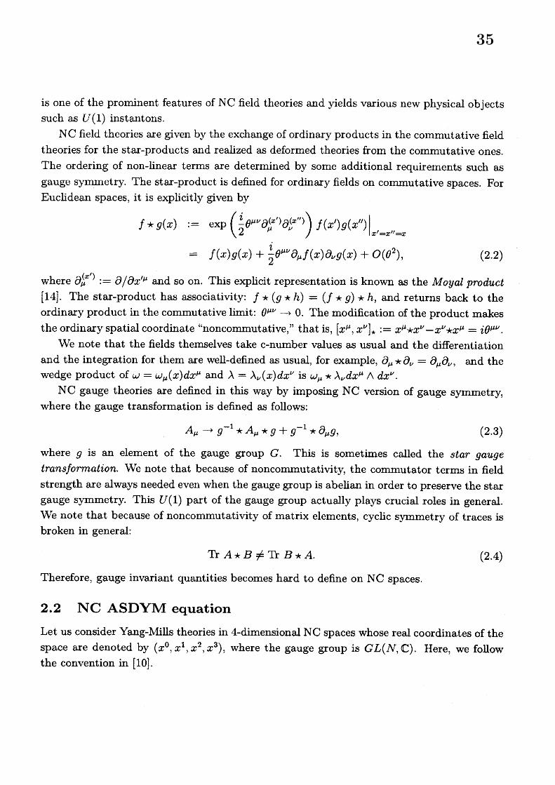
is one of the prominent features of NC field theories and yields various new physic$al$ objectssuch as $U(1)$ instantons.

NC field theories are given by the exchange of ordinary products in the commutative fieldtheories for the star-products and realized as deformed theories from the commutative ones.The ordering of non-linear terms are determined by some additional requirements such asgauge symmetry. The star-product is defined for ordinary fields on commutative spaces. ForEuclidean spaces, it is explicitly given by

$f\star g(x)$ $;= \exp(\frac{i}{2}\theta^{\mu\nu}\partial_{\mu}^{(x’)}\partial_{\nu}^{(x’’)})f(x’)g(x’’)|_{x’=x’’\supset}$

$=$ $f(x)g(x)+ \frac{i}{2}\theta^{\mu\nu}\partial_{\mu}f(x)\partial_{\nu}g(x)+O(\theta^{2})$ , (2.2)

where $\partial_{\mu}^{(x’)}$$:=\partial/\partial x^{\prime\mu}$ and so on. This explicit representation is known as the Moyal product

[14]. The star-product has associativity: $f\star(g\star h)=(f\star g)\star h$ , and returns back to theordinary product in the commutative limit: $\theta^{\mu\nu}arrow 0$ . The modification of the product makesthe ordinary spatial coordinate “noncommutative,” that is, $[x^{\mu}, x^{\nu}]_{\star}$ $:=x^{\mu}\star x^{\nu}-x^{\nu}\star x^{\mu}=i\theta^{\mu\nu}$.

We note that the fields themselves take c-number values as usual and the differentiationand the integration for them are $weU$-defined as usual, for example, $\partial_{\mu}\star\partial_{\nu}=\partial_{\mu}\partial_{\nu}$ , and thewedge product of $\omega=\omega_{\mu}(x)dx^{\mu}$ and $\lambda=\lambda_{\nu}(x)dx^{\nu}$ is $\omega_{\mu}\star\lambda_{\nu}dx^{\mu}\wedge dx^{\nu}$ .

NC gauge theories are defined in this way by imposing NC version of gauge symmetry,where the gauge transformation is defined as follows:

$A_{\mu}arrow g^{-1}\star A_{\mu}\star g+g^{-1}\star\partial_{\mu}g$ , (2.3)

where $g$ is an element of the gauge group $G$ . This is sometimes called the star gaugetransformation. We note that because of noncommutativity, the commutator terms in fieldstrength are always needed even when the gauge group is abelian in order to preserve the stargauge $s$)$mmetry$. This $U(1)$ part of the gauge $oup$ actually plays crucial roles in general.We note that because of noncommutativity of matrix elements, cyclic symmetry of traces isbroken in general:

Tr $A\star B\neq$ Thr $B\star$ A. (2.4)

Therefore, gauge invariant quantities becomes hard to define on NC spaces.

2.2 NC ASDYM equation

Let us consider Yang-Mills theories in 4-dimensional NC spaces whose real coordinates of thespace are denoted by $(x^{0}, x^{1}, x^{2}, x^{3})$ , where the gauge group is $GL(N, \mathbb{C})$ . Here, we foUowthe convention in [10].

35

First, we introduce double null coordinates of 4-dimensional space as follows

$ds^{2}=2(dzdZ-dwdw$ , (2.5)

We can recover various kind of real spaces by putting the corresponding reality conditionson the double null coordinates $z,\tilde{z},$ $w,\tilde{w}$ as follows:

$\bullet$ Euclidean Space $(\overline{w}=-\tilde{w}:\overline{z}=\tilde{z})$ : An example is

$(\tilde{w}\tilde{z}wz$ $= \frac{1}{\sqrt{2}}(X^{0}x^{2}I_{ix^{3}}^{ix^{1}}$$-(x^{2}-ix^{3})x^{0}-ix^{1}$ (2.6)

$\bullet$ Minkowski Space ( $\overline{w}=\tilde{w};z$ and $\tilde{z}$ are real.): An example is

$(\tilde{w}\tilde{z}wz$ $= \frac{1}{\sqrt{2}}(x^{2}+ix^{3}x^{0}+x^{1}x^{2}-ix^{3}x^{0}-x^{1}$ (2.7)

$\bullet$ Ultrahyperbolic Space $(\overline{w}=\tilde{w};\overline{z}=\tilde{z})$ : An example is

$(\begin{array}{ll}\tilde{z} v_{j}\cdot\tilde{w} z\end{array})=\frac{1}{\sqrt{2}}(\begin{array}{ll}x^{0}+ix^{1} x^{2}-ix^{3}x^{2}+ix^{3} x^{0}-ix^{1}\end{array})$ . (2.8)

For Euclidean and ultrahyperbolic signatures, Hodge dual operator $*satisfies*^{2}=1$

and hence the space of 2-forms $\beta$ decomposes into the direct sum of eigenvalues of $*$ witheigenvalues $\pm 1$ , that is, self-dual (SD) part $(*\beta=\beta)$ and anti-self-dual (ASD) part $(*\beta=$

$-\beta)$ . $\mathbb{R}om$ now on, we treat these two signatures.NC ASDYM equation is derived from compatibility condition of the following linear

system:

$L\star\Psi$ $:=$ $(D_{w}-\lambda D_{\tilde{z}})\star\Psi=(\partial_{w}+A_{w}-\lambda(\partial_{\overline{z}}+\mathcal{A}_{\tilde{z}}))\star\Psi(x;\lambda)=0$ ,$M\star\Psi$ $:=$ $(D_{z}-\lambda D_{\tilde{w}})\star\Psi=(\partial_{z}+A_{z}-\lambda(\partial_{\overline{w}}+A_{\tilde{\omega}}))\star\Psi(x;\lambda)=0$ , (2.9)

where $A_{z},$ $A_{w},$ $A_{\tilde{z}},$ $A_{2\overline{L}}$, and $D_{z},$ $D_{w},$ $D_{\tilde{z}},$ $D_{\tilde{w}}$ denote gauge fields and covariant derivatives inthe Yang-Mills theory, respectively. The constant $\lambda$ is caUed the spectral parameter. Thecompatible condition $[L,$ $M|_{\star}=0$ gives rise to a quadratic polynomial of $\lambda$ and each coefficientyields NC ASDYM equations whose explicit representations are as follows:

$F_{wz}$ $=\partial_{w}A_{z}-\partial_{z}A_{w}+[A_{\psi)}A_{z}]_{\star}=0$,

$F_{\tilde{w}\tilde{z}}=\partial_{\tilde{w}}A_{\tilde{z}}-\partial_{\tilde{z}}A_{\tilde{w}}+[A_{\tilde{w}},$ $A_{\tilde{z}}|_{\star}=0$ ,

$F_{z_{\tilde{k}}^{-}}-F_{u’\tilde{u}}$, $=\partial_{z}A_{\tilde{z}}-\partial_{\tilde{L}}\sim A_{z}+\partial_{\tilde{w}}A_{u}|-\partial_{w}A_{\tilde{w}}+[A_{z}, A_{\overline{z}}]_{\star}-[A_{w},$ $A_{\overline{w}}|_{\star}=0$ . (2.10)

36

2.3 NC Yang’s equation and $J$, K-matricesHere we discuss the potential forms of NC ASDYM equations such as NC $J$, K-matrix for-malisms and NC Yang’s equation, which is already presented by e.g. K. Takasaki [32].

Let us first discuss the $J$-matnx formalism of NC ASDYM equation. The first equationof NC ASDYM equation (2.10) is the compatible condition of $D_{z}\star h=0,$ $D_{w}\star h=0$ , where$h$ is a $N\cross N$ matrix. Hence we get

$A_{z}=-h_{z}\star h^{-1}$ , $A_{w}=-h_{w}\star h^{-1}$ , (2.11)

where $h_{x}$ $:=\partial h/\partial z,$ $h_{w}$ $:=\partial h/\partial w$ . Similarly, the second eq. of NC ASDYM equation (2.10)leads to

$A_{k}\approx=-\tilde{h}_{\tilde{z}}\star\tilde{h}^{-1}$ , $A_{\overline{w}}=-\tilde{h}_{\overline{w}}\star\tilde{h}^{-1}$ , (2.12)

where $\tilde{h}$ is also a $NxN$ matrix. By defining $J=\tilde{h}^{-1}\star h$ , the third eq. of NC ASDYMequation (2.10) becomes NC Yang$\rangle s$ equation

$\partial_{z}(J^{-1}\star\partial_{\tilde{z}}J)-\partial_{w}(J^{-1}\star\partial_{\overline{w}}J)=0$. (2.13)

3 NC CFYG transformation and NC Atiyah-Ward AnsatzHere we present a NC version of the Corrigan-Fairlie-Yates-Goddard (CFYG) transformation[50] which leaves NC Yang’s equation for $G=GL(2)$ as it is. The NC CFYG transformationgenerates some class of exact solutions which belong to NC version of the Atiyah-Ward ansatz[16] labeled by a positive integer $m=1,2,3,$ $\cdots$ . Origin of these results will be clarified inthe next section.

In order to discuss it, we have to rewrite a generic $2\cross 2$ matrix $J$ as follows:

$J=(f-g\star b^{-1}\star eb^{-1}\star e$ $-g\star b^{-1}b^{-1}$ , (3.1)

$wheref\sim$ and $b$ are non-singular. This parameterization comes from a gauge fixing where $h$

and $h$ are lower-triangular and upper-triangular, respectively, such that,

$J=\tilde{h}^{-1}\star h=(01gb$ $-1\star(\begin{array}{ll}f 0e 1\end{array})=(f-g\star b^{-1}\star eb^{-1}\star e-g\star b^{-1}b^{-1}$ (3.2)

Hence, the inverse of $J$ has a similar form:

$J^{-1}=h^{-1}\star\tilde{h}=(fe01$ $-1\star(01gb$ $=(_{-e\star f^{-1}}f^{-1}$ $b-e\star f^{-1}\star gf^{-1}\star g$ (3.3)

37

With this decomposition, NC Yang’s equation (2.13) becomes

$\partial_{z}(f^{-1}\star g_{\tilde{z}}\star b^{-1})-\partial_{w}(f^{-1}\star g_{\tilde{w}}\star b^{-1})$ $=0$ ,$\partial_{\tilde{z}}(b^{-1}\star e_{z}\star f^{-1})-\partial_{\tilde{w}}(b^{-1}\star e_{w}\star f^{-1})$ $=0$ ,

$\partial_{z}(b_{\tilde{z}}\star b^{-1})-\partial_{w}(b_{u\tilde{)}}\star b^{-1})-e_{z}\star f^{-1}\star g_{\tilde{z}}\star b^{-1}+e_{w}\star f^{-1}\star g_{\tilde{w}}\star b^{-1}$ $=0$ ,$\partial_{z}(f^{-1}\star f_{\tilde{z}})-\partial_{w}(f^{-1}\star f_{\overline{w}})-f^{-1}\star g_{\tilde{z}}\star b^{-1}\star e_{z}+f^{-1}\star g_{\tilde{w}}\star b^{-1}\star e_{w}$ $=0$ . (3.4)

By using these formulae, we can find the gauge fields and the field strength in terms of$b,$ $e,$ $f,$ $g$ .

3.1 NC CFYG transformation

Now we describe the NC CFYG transformation explicitly. It is a composition of the followingtwo B\"acklund transformations for the decomposed NC Yang’s equations (3.4).

$\bullet$ $\beta$-transformation [10, 3]:

$e_{w}^{new}=f^{-1}\star g_{\tilde{z}}\star b^{-1},$ $e_{z}^{new}=f^{-1}\star g_{\tilde{u}}|\star b^{-1}$ ,$g_{\tilde{z}}^{new}=b^{-1}\star e_{w}\star f^{-1},$ $g_{\tilde{w}}^{new}=b^{-1}\star e_{z}\star f^{-1}$ ,

$f^{new}=b^{-1},$ $b^{new}=f^{-1}$ .

The first four equations can be interpreted as integrability conditions for the first twoequations in (3.4). We can easily check that the last two equations in (3.4) are invariantunder this transformation. Also, it is clear that $\beta$-transformation is involutive, that is,$\beta\circ\beta$ is the identity transformation.

$\bullet$

$\gamma_{0}$-transformation:

$(f^{new}e^{new}g^{new}b^{new}$ $=(\begin{array}{ll}b eg f\end{array})=((e-b\star g^{-1}\star f)^{-1}(b-e\star f^{-1}\star g)^{-1}$ $(f-g:b^{-1}\star e)^{-1}(g-fe^{-1}\star b)^{-1}$ . (3.5)

This follows from the fact that the transformation $\gamma 0$ : $J\mapsto J^{new}$ is equivalent to thesimple conjugation $J^{new}=C_{0}^{-1}JC_{0},$ $C_{0}=(\begin{array}{ll}0 11 0\end{array})$ , which clearly leaves the NCYang’s equation (2.13) invariant. The relation (3.5) is derived by comparing elementsin this transformation. It is a trivial fact that $\gamma_{0}$-transformation is also involutive.

3.2 Exact NC Atiyah-Ward ansatz solutions

Now we construct exact solutions by using a chain of B\"acklund transformations bom a seedsolution. Let us consider $b=e=f=g=\Delta_{0}^{-1}$ , then we can easily find that the decomposed

38

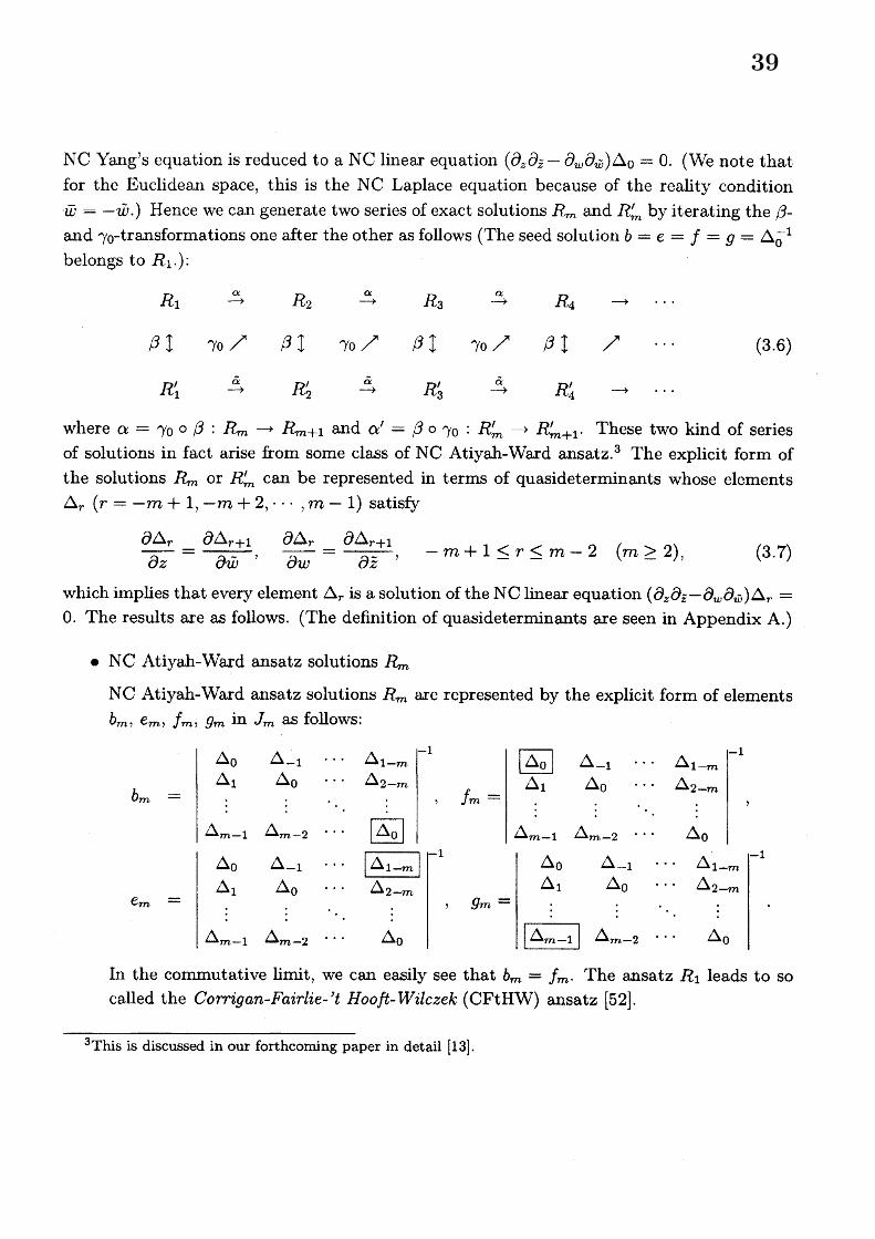
NC Yang’s equation is reduced to a NC linear equation $(\partial_{z}\partial_{\overline{z}}-\partial_{w}\partial_{\overline{w}})\Delta_{0}=0$ . (We note thatfor the Euclidean space, this is the NC Laplace equation because of the reality condition$\overline{w}=-\tilde{w}.)$ Hence we can generate two series of exact solutions $R_{m}$ and $R_{m}’$ by iterating the $\beta-$

and $\gamma_{0}$-transformations one after the other as follows (The seed solution $b=e=f=g=\Delta_{0}^{-1}$

belongs to $R_{1}.$ ):

$R_{1}$$arrow\alpha$

$R_{2}$$arrow\alpha$

$R_{3}$$arrow\alpha$

$R_{4}$ $arrow$ . . .

$\beta$ I $\gamma_{0}\nearrow$ $\beta\downarrow$ $\gamma_{0}\nearrow$ $\beta$ I $\gamma_{0}\nearrow$ $\beta$ I $\nearrow$ (3.6)

$R_{1}’$$arrow\tilde{\alpha}$

$R_{2}’$$arrow\tilde{\alpha}$

$R_{3}’$$arrow\tilde{\alpha}$

$R_{4}’$ $arrow$ . . .

where $\alpha=\gamma_{0}0\beta$ : $R_{m}arrow R_{m+1}$ and $\alpha’=\beta 0\gamma_{0}$ : $R_{m}’arrow R_{m+1}’$ . These two kind of seriesof solutions in fact arise $hom$ some class of NC Atiyah-Ward ansatz.3 The explicit form ofthe solutions $R_{m}$ or $R_{m}’$ can be represented in term of quasideterminants whose elements$\Delta_{r}(r=-m+1, -m+2, \cdots, m-1)$ satisfy

$\frac{\partial\Delta_{r}}{\partial z}=\frac{\partial\Delta_{r+1}}{\partial\tilde{w}}$ , $\frac{\partial\Delta_{r}}{\partial w}=\frac{\partial\Delta_{r+1}}{\partial\tilde{z}}$ , $-m+1\leq r\leq m-2$ $(m\geq 2)$ , (3.7)

which implies that every element $\Delta_{r}$ is a solution of the NC linear equation $(\partial_{z}\partial_{k}\approx-\partial_{w}\partial_{\overline{w}})\Delta_{r}=$

$0$ . The results are as follows. (The definition of quasideterminants are seen in Appendix A.)

$\bullet$ NC Atiyah-Ward ansatz solutions $R_{m}$

NC Atiyah-Ward ansatz solutions $R_{m}$ are represented by the explicit form of elements$b_{m},$ $e_{m},$ $f_{m},$ $g_{m}$ in $J_{m}$ as follows:

$b_{m}$ $=$ $\Delta_{m-1}\Delta_{0}\Delta_{1}$

:$\Delta_{m-2}\Delta_{-1}\Delta_{0}$

:

$..\cdot.\cdot$

. $\Delta_{1-m}\Delta_{2.-m}\Delta_{0}:|\begin{array}{ll}-1 ,f_{m}=\end{array}|-1\Delta_{1}$$\Delta_{m-2}\Delta_{-1}\Delta_{0}$

$..\cdot.\cdot$

$\Delta_{2.\cdot.-m}\Delta_{1-m}\Delta_{0}|_{-1}^{-1}$

$\Delta_{0}$ $\Delta_{-1}$ . . . $\Delta_{1-m}$ $\Delta_{0}$ $\Delta_{-1}$ . . . $\Delta_{1-m}$

$\Delta_{1}$ $\Delta_{0}$ . . . $\Delta_{2-m}$$\Delta_{1}$ $\Delta_{0}$ . . . $\Delta_{2-m}$

$e_{m}$ $=$ , $g_{m}=$

. . ... . .. ... .

$\Delta_{m-1}$ $\Delta_{m-2}$ . .. $\Delta_{0}$ $\Delta_{m-1}$ $\Delta_{m-2}$ . . . $\Delta_{0}$

In the commutative limit, we can easily see that $b_{m}=f_{m}$ . The ansatz $R_{1}$ leads to socalled the Cowigan-Fairlie-,t Hoofl-Wilczek (CFtHW) ansatz [52].

3This is discussed in our forthcoming paper in detail $[$ 13$]$ .

39

$\bullet$ NC Atiyah-Ward ansatz solutions $R_{m}’$

NC Atiyah-Ward ansatz solutions $R_{m}’$ are represented by the explicit form of elements$b_{m}’,$ $e_{m}’,$ $f_{m}’,$ $g_{m}’$ in $\tilde{J}_{m}$ as follows:

$b_{m}’$ $=$ $\Delta_{m-1}\Delta_{1}\Delta_{0}$

:$\Delta_{m-2}\Delta_{-1}\Delta_{0}$

: $.\cdot.\cdot\cdot$

$\Delta_{2.-m}\Delta_{1-m}\Delta_{0}:|$ , $f_{m}’=|_{\Delta_{m-1}}^{\Delta_{1}}\Delta_{0}$ $\Delta_{m-2}\Delta_{-1}\Delta_{0}$

$...\cdot$

.

$\Delta_{2.,..-\eta 1}\Delta_{1-m}\Delta_{0}$

’

$e_{m}’$ $=$

$\Delta_{-1}$ $\Delta_{-2}$ . . . $\Delta_{-m}$ $\Delta_{1}$ $\Delta_{0}$ . . . $\Delta_{2-m}$

$\Delta_{0}$ $\Delta_{-1}$ . . . $\Delta_{1-m}$$\Delta_{2}$ $\Delta_{1}$ . . . $\Delta_{3-m}$

$g_{m}’=$:. : :. : : .. :... ..$\Delta_{m-2}\Delta_{m-3}$ . . . $\Delta_{-1}$ $\Delta_{m}$ $\Delta_{m-1}$ . . . $\Delta_{1}$

In the commutative case, $b_{m}’=f_{m}’$ also holds. For $m=1$ , we get $b_{1}’=f_{1}’=\Delta_{0},$ $e_{1}’=$

$\Delta_{-1},$ $g_{1}’=\Delta_{1}$ and then the relation (3.7) implies that $e_{1,z}’=f_{1,\tilde{w}}’,$ $e_{1,w}’=f_{1,\overline{z}}’,$ $f_{1z}’$)

$=$

$g_{1,\tau\tilde{1}^{1}}’,$ $f_{1.w}’=g_{1,\tilde{z}}’$ , and leads to the CFtHW ansatz which was first pointed out by Yang[53].

The proof of these results [12] can be made by using identities of quasideterminants, suchas, NC Jacobi identity, homological relations, and Gilson-Nimmo’s derivative formula as inAppendix A. This implies that $NC$ Backlund transformations are identities of quasidetermi-nants.

We can also present a compact form of the whole Yang’s matrix $J$ in terms of a singlequasideterminants expanded by a $2\cross 2$ submatrix. For example, the solution in $R_{m}’$ leads to

(3.8)

where

$a_{21}$ $a_{22}$ $a_{23}$ $a_{24}$

$a_{11}$ $a_{12}$ $a_{13}$

$a_{34}a_{14}a_{44}$ $:=$ $[|_{a_{41}}^{a}a_{11}a_{31}a_{21}a_{21}11$$a_{22}a_{32}a_{12}a\iota 2a_{22}a_{42}$

$\underline{\frac{\prod}{\prod a_{13}a_{23}}a_{23}aa_{33}a_{43}13}|$ $|\begin{array}{lll}a_{11} a_{12} a_{14}a_{21} a_{22} a_{24}a_{31} a_{32} a_{34}a_{11} a_{12} a_{14}a_{2l} a_{22} a_{24}a_{41} a_{42} a_{44}\end{array}|]$ .$a_{31}$ $a_{32}$ $a_{33}$

$a_{41}$ $a_{42}$ $a_{43}$

40

Because $J$ is gauge invariant, this shows that the present B\"acklund transformation is notjust a gauge transformation but a non-trivial one. The proof of these representations is givenin Appendix A in $[$ 12] and in [60].

4 Twistor descriptions of NC ASDYM equations

In this section, we give an origin of the B\"acklund transformations for NC ASDYM equa-tions and NC Atiyah-Ward ansatz solutions from the geometrical viewpoint of NC twistortheory. NC twistor theory has been developed by several authors and the mathematicalfoundation is established $[31]-[38]$ . Here we just need one-to-one correspondence between aNC ASDYM connection and a Patching matrix $P$ of “NC holomorphic vector bundle on aNC 3-dimensional projective space. The holomorphy implies

$P=P(\zeta w+\tilde{z}, \zeta z+\tilde{w}, \zeta)$ . (4.1)

We note that noncommutativity can be introduced into only two variables $\zeta w+\tilde{z},$ $\zeta z+\tilde{w}$ .Then $\zeta$ is a commutative variable and steps of solving Riemann-Hilbert problem becomesiniilar to commutative one. However the noncommutativity in the first and second coordi-nates introduce nontrivial effects in the ASDYM connections and give rise to new physicalobjects, such as $U(1)$ instantons. Original results in this section are due to our forthcomingpaper [13].

4.1 Riemann-Hilbert problem for NC Atiyah-Ward AnsatzThe solution $\psi$ ($NxN$ matrix) of the linear system (2.9) is not regular at $\zeta=\infty$ becauseof Liouville’s theorem. Hence we have to consider another linear system on another localpatCh whose coordinate $\tilde{\zeta}=1/\zeta$ as

$\tilde{\zeta}D_{w}\star\tilde{\psi}-D_{\tilde{z}}\star\tilde{\psi}=0$ ,$\tilde{\zeta}D_{\tilde{4}}\star\tilde{\psi}-D_{\tilde{w}}\star\tilde{\psi}=0$. (4.2)

Then we can prove that if the patching matrix $P$ can be factorized as follows:

$P(\zeta w+\tilde{z}, \zeta z+\tilde{w}, \zeta)=\tilde{\psi}^{-1}(x;\zeta)\star\psi(x;\zeta)$ . (4.3)

where $\psi$ and $\tilde{\psi}$ are regular near $\zeta=0$ and $\zeta=\infty$ , respectively, then the $\psi$ and $\tilde{\psi}$ are thesolutions of the linear systems for NC ASDYM equation.

Hence if we solve the factorization problem (or the Riemann-Hilbert problem) (4.3), thenwe can reproduce ASDYM connections in terms of $h$ and $\tilde{h}$ by using (2.11), (2.12) and thefact $h(x)=\psi(x, \zeta=0),\tilde{h}(x)=\tilde{\psi}(x, \zeta=\infty)$ .

41

From now on, we restrict ourselves to $G=GL(2)$ . In this case, we can take a simpleansatz for the Patching matrix $P$ , which is called the Atiyah-Ward ansatz in commutativecase [16]. NC generalization of this ansatz is straightforward and actually leads to a solutionof the factorization problem. The l-th order NC Atiyah-Ward ansatz is specified by thefollowing form of the patching matrix $(l=1,2, \cdots)$ :

$P(x;\zeta)=(\begin{array}{ll}0 \zeta^{-l}\zeta^{l} \Delta(x\cdot\zeta)\end{array})$ . (4.4)

We note that holomorphy of $P$ implies $\Delta(x;\zeta)=(\zeta w+\tilde{z}, \zeta z+\tilde{w}, \zeta)$ , or equivalently, $(\partial_{w}-$

$\zeta\partial_{\overline{z}})\Delta=0,$ $(\partial_{z}-\zeta\partial_{\tilde{w}})\Delta=0$ . Hence, the Laurent expansion of $\Delta$ w.r.t. $\zeta$

$\delta(x;\zeta)=\sum_{i=-\infty}^{\infty}\Delta_{i}(x)\zeta^{-i}$ , (4.5)

gives rise to the following relations in the coefficients as

$\frac{\partial\Delta_{i}}{\partial z}=\frac{\partial\Delta_{i+1}}{\theta\tilde{w}}$, $\frac{\partial\Delta_{i}}{\partial w}=\frac{\partial\Delta_{i+1}}{\partial\tilde{z}}$ , (4.6)

which coincide with the chasing relation (3.7). We will soon see that the coefficients $\Delta_{i}(x)$

are the scalar functions in the solutions generated by the B\"acklund transformations in theprevious section.

Now let us solve the factorization problem $\tilde{\psi}\star P=\psi$ for the NC Atiyah-Ward ansatz,which is concretely written down as

$(\tilde{\psi}_{21}\tilde{\psi}_{11}$ $\tilde{\psi}_{22}^{12}\tilde{\psi})\star(\begin{array}{ll}0 \zeta^{-l}\zeta^{l} \Delta(x\cdot\zeta)\end{array})=(\psi_{21}\psi_{11}$ $\psi_{12}\psi_{22}$ , (4.7)

that is,

$\tilde{\psi}_{12}\zeta^{l}=\psi_{11}$ , $\tilde{\psi}_{22}\zeta^{l}=\psi_{21}$ , (4.8)$\tilde{\psi}_{11}\zeta^{-t}+\tilde{\psi}_{12}\star\Delta=\psi_{12}$ , $\tilde{\psi}_{21}\zeta^{-l}+\tilde{\psi}_{22}\star\Delta=\psi_{22}$ . (4.9)

From Eq. (4.8) together with the relation between $\psi,\tilde{\psi}$ and $h,\tilde{h}$ , we find that some compo-nents become polynomials w.r. $t$ . $\zeta$ :

$\psi_{11}$ $=h_{11}+a_{1}\zeta+a_{2}\zeta^{2}+\cdots a_{l-1}\zeta^{l-1}+\tilde{h}_{12}\zeta^{l}$ ,$\psi_{21}$ $=h_{21}+b_{1}\zeta+b_{2}\zeta^{2}+\cdots b_{l-1}\zeta^{\iota_{-1}}+\tilde{h}_{22}\zeta^{l}$ ,$\tilde{\psi}_{12}$ $=\tilde{h}_{12}+a_{l-1}\zeta^{-1}+a_{l-2}\zeta^{-2}+\cdots a_{1}\zeta^{1-l}+h_{11}\zeta^{-l}$ ,$\tilde{\psi}_{22}$ $=$ $\tilde{h}_{22}+b_{l-1}\zeta^{-1}+b_{l-2}\zeta^{-2}+\cdots+b_{1}\zeta^{1-l}+h_{21}\zeta^{-l}$ , (4.10)

42

and so on. By substituting these relations into Eq. (4.9), we get sets of equations for $h$ and$\tilde{h}$ in the coefficients of $\zeta^{0},$ $\zeta^{-1}$ . $\cdot\cdot\cdot$ , $\zeta^{-l}$ :

$h_{11}$ $=$ $h_{12}\star|D_{l+1}|_{l+1,1}^{-1}-\tilde{h}_{11}\star|D_{l+1}|_{l+1,l+1}^{-1}$ ,$h_{21}$ $=$ $h_{22}\star|D_{l+1}|_{l+1,1}^{-1}-\tilde{h}_{21}\star|D_{l+1}|_{l+1,l+1}^{-1}$ ,$\tilde{h}_{12}$ $=$ $h_{12}\star|D_{l+1}|_{11}^{-1})-\tilde{h}_{11}\star|D_{l+1}|_{1_{l}l+1}^{-1}$ ,$\tilde{h}_{22}$ $=$ $h_{22}\star|D_{l+1}|_{1,1}^{-1}-\tilde{h}_{21}\star|D_{l+1}|_{1,l+1}^{-1}$ ,

(4.11)

where

$D_{l}$ $:=(\Delta_{l-1}\Delta_{1}\Delta_{0}$ $\Delta_{l-2}\Delta_{-1}\Delta_{0}$

$.\cdot.\cdot$

.

$\Delta_{2-l}\Delta_{1-l}\Delta_{0}$ (4.12)

By taking some gauge condition, Eq. (4.11) can be solved for $h$ and $\tilde{h}$ in terms of quaside-terminants of $D_{l+1}$ , which just coincide with the generated solutions by the B\"acklund trans-formation in the previous section ! This is an origin of the NC Atiyah-Ward solutions.

4.2 Origin of the NC CFYG transformation

Finally let us discuss an origin of the NC CFYG transformations, $\beta$-transformation and$\gamma_{0}$-transformation. These transformations can be viewed as adjoint actions for the patchingmatrix $P$ :

$\beta:P\mapsto P^{new}=B^{-1}PB$ , $\gamma_{0}:P\mapsto P^{new}=C^{-1}PC$, (4.13)

where

$B=(\zeta^{-1}0$ $01$ , $C_{0}=(\begin{array}{ll}0 11 0\end{array})$ . (4.14)

together with a singular gauge transformation for $\beta$-transformation. It is clear that thisleads to $\gamma_{0}$-transformation by considering the action of $C$ for $\psi$ and $\tilde{\psi}$ . The action of $B$ isdefined at the level of $\psi$ and $\tilde{\psi}$ as follows:

$\psi^{new}=s\star\psi B$ , $\tilde{\psi}^{new}=s\star\tilde{\psi}B$ , (4.15)

where

$s=(_{-f^{-1}}0$$\zeta b^{-1}$

(4.16)$0$

43

The explicit calculation gives

$\psi^{new}=(_{-\zeta^{-1}f^{-1}\star\psi_{12}}b^{-1}\psi_{22}$ $-\zeta b^{-1}\star\psi_{21}f^{-1}\star\psi_{11}$ (4.17)

where $\psi_{ij}$ is the $(i, j)-$th element of $\psi$ . In the $\zetaarrow 0$ limit, this reduces to

$h^{new}=(f^{new}e^{new}01$ $=(\begin{array}{ll}b^{-l} 0-f^{-1}\star j_{12} 1\end{array})$ , (4.18)

where $\psi=h+j\zeta+\mathcal{O}(\zeta^{2})$ .

Here we note that the linear systems can be represented in terms of $b,$ $f,$ $e,$ $g$ as

$L\star\psi$ $=$ $(\partial_{w}-\zeta\partial_{\tilde{z}})\star\psi+(:$ $\zeta g_{\tilde{z}}\zeta b_{\tilde{z}};_{b^{-1}}^{b^{-1}})\star\psi=0$ ,

$M\star\psi=$ $(\partial_{z}-\zeta\partial_{\tilde{w}})\star\psi+(\begin{array}{lllll}-f_{z} \star f^{-1} \zeta g_{\tilde{w}}\star b^{-1}-e_{z} \star f^{-1} \zeta b_{\tau\tilde{\iota}},\star b^{-1}\end{array})\star\psi=0$ . (4.19)

By picking the first order term of $\zeta$ in the 1-2 component of the first equation, we get

$\partial_{w}(f^{-1}\star j_{12})=-f^{-1}\star g_{\overline{z}}\star b^{-1}$. (4.20)

Hence from the 1-1 and 2-1 components of Eq. (4.18), we have

$f^{new}=b^{-1}$ , $\partial_{w}e^{new}=-\partial_{w}(f^{-1}\star j_{12})=f^{-1}\star g_{\tilde{z}}\star b^{-1}$ , (4.21)

which are just parts of the $\beta$-transformation (3.5). In similar way, we can get the otherones. Therefore the $\beta$-transformation (3.5) can be interpreted as the transformation of thepatching matrix $F\mapsto B^{-1}FB$ together with the singular gauge transformation $s$ .

5 NC Ward’s Conjecture

Here we briefly discuss reductions of NC ASDYM equation into lower-dimensional NC inte-

grable equations such as the NC $KdV$ equation. let us summarize the strategy for reductionsof NC ASDYM equation into lower-dimensions. Reductions are classified by the following

ingredient$s$ :

$\bullet$ A choice of gauge group

$\bullet$ A choice of symmetry, such as, translational symmetry

$\bullet$ A choice of gauge fixing

44

$\bullet$ A choice of constants of integrations in the process of reductions

Gauge groups are in general $GL(N)$ . We have to take $U(1)$ part into account in NC case.A choice of symmetry reduces NC ASDYM equations to simple forms. We note that non-commutativity must be eliminated in the reduced directions because of compatibility withthe symnietry. Hence within the reduced directions, discussion about the symnetry is thesame as commutative one. A choice of gauge fixing is the most important ingredient in thispaper which is shown explicitly at each subsection. The residual gauge symmetry sometimesshows equivalence of a few reductions. Constants of integrations in the process of reductionssometimes lead to parameter families of NC reduced equations, however, in this paper, weset all integral constants zero for simplicity.

5.1 Reduction to the NC $KdV$ Equation

In this section, we present non-trivial reductions of NC ASDYM equation with $G=GL(2)$to the NC $KdV$ equation.

First, let us take a dimensional reduction by null translations:

$X=\partial_{w}-\partial_{\tilde{w}},$ $Y=\partial_{\overline{z}}$ . (5.1)

Then the gauge field A. becomes a Higgs field which is denoted by $\Phi_{\overline{z}}$ . Here let us take agauge fixing of $\Phi_{\tilde{z}}$ as follows:

$\Phi_{\tilde{z}}=(\begin{array}{ll}0 01 0\end{array})$ .

Then the NC ASDYM equation is simply reduced:

$\Phi_{\tilde{z}}’+[A_{u^{-}}|, \Phi_{\overline{z}}]_{\star}=0$ ,$\dot{\Phi}_{\tilde{z}}+A_{w}’-A_{\tilde{w}}’+[A_{z}, \Phi_{\tilde{z}}]_{\star}-[A_{u},, A_{\tilde{w}}]_{\star}=0$,$A_{\wedge}^{l}\sim-\dot{A}_{w}+[A_{w}, A_{z}]_{\star}=0$, (5.2)

where $(t, x)\equiv(z, w+\tilde{w})$ and $\dot{f}$ $:=\partial f/\partial t,$ $f’$ $:=\partial f/\partial x$ .Now let us take the following non-trivial reduction conditions for the gauge fields

$A_{\overline{w}}=0,$ $\Phi_{\tilde{z}}=(\begin{array}{ll}0 01 0\end{array}),$ $A_{w}=(\begin{array}{ll}q -1q’+q\star q -q\end{array})$ ,

$A_{z}= \frac{1}{2}((1/2)q^{\prime l/}+q’\star q’+q\star q’+q’’\star q+2q\star q’\star qq’’+2q_{J}’\star q-q’’-2q\star q’-2q’$ (5.3)

45

These conditions automatically solve the first and second equations in (5.2) and the thirdone gives rise to NC potential $KdV$ equation

$\dot{q}=\frac{1}{4}q’’’+\frac{3}{2}(q\star q)’$ (5.4)

which is derived from NC $KdV$ equation with $u=2q’$

$\dot{u}=\frac{1}{4}u’’’+\frac{3}{4}(u’\star u+u\star u’)$ . (5.5)

In this way, NC $KdV$ equation is actually derived. We note that the gauge group is not$SL(2)$ but $GL(2)$ because $A_{z}$ is not traceless. This implies $U(1)$ part of the gauge groupplays a crucial role in the reduction also.

This NC $KdV$ equation has been studied by several authors and proved to possess infiniteconserved quantities [58] in terms of Strachan products [40] and exact multi-soliton solutionsin terms of quasideterminants also [41, 27]. (See also [56, 57].)

6 Conclusion and Discussion

In this article, we have presented B\"acklund transformations for the NC ASDYM equationwith $G=GL(2)$ and constructed $hom$ a simple seed solution a series of exact NC Atiyah-Ward ansatz solutions expressed explicitly in terms of quasideterminants. We have alsodiscussed the origin of this transformation in the framework of NC twistor theory.

These results could be applied also to lower-dimensional systems via the results on theNC Ward’s conjecture including NC monopoles, NC $KdV$ equations and so on, and mightshed light on a profound connection between higher-dimensional integrable systems relatedto twistor theory and lower-dimensional ones related to Sato’s theory.

Acknowledgments

The author would like to thank C. R. Gilson and J. J. C. Nimmo for collaboration and hos-pitality during stay at Department of Mathematics, University of Glasgow, and L. Mason fora lot of helpful discussion and hospitality during stay at Mathematical Institute, Universityof Oxford, and the organizers of the present conference for invitation and hospitality. Thiswork was supported by the Yamada Science Foundation for the promotion of the naturalscience and Grant-in-Aid for Young Scientists (#18740142),

46

A Brief Review of Quasideterminants

In this appendix, we make a brief introduction of quasi-determinants introduced by Gelfandand Retakh in 1992 [11] and present a few properties of them which play important rolesin the main sections. Relation between quasi-determinants and noncommutative symmetricfunctions is seen in e.g. $[$59$]$ .

Quasi-determinants are not just a noncommutative generalization of usual commutativedeterminants but rather related to inverse matrices.

Let $A=(a_{ij})$ be a $n\cross n$ matrix and $B=(b_{ij})$ be the inverse matrix of $\mathcal{A}$ . Here all matrixelements are supposed to belong to a (noncommutative) ring with an associative product.This general noncommutative situation includes the Moyal or NC deformation.

Quasi-determinants of $A$ are defined formally as the inverse of the elements of $B=A^{-1}$ :

$|A|_{ij}$ $:=b_{ji}^{-1}$ . (A.1)

In the commutative linut, this is reduced to

$|A|_{ij} arrow(-1)^{i+j}\frac{\det A}{\det\tilde{A}^{ij}}$ , (A.2)

where $\tilde{A}^{ij}$ is the matrix obtained $hom$ $A$ deleting the i-th row and the j-th column.We can write down more explicit form of quasi-determinants. In order to see it, let us

recall the following formula for a square matrix:

$(\begin{array}{ll}A BC D\end{array})=(_{-(D-CA^{-1}B)^{-1}CA^{-1}}(A-BD^{-1}C)^{-1}$ $-A^{-1}B(D-CA^{-1}B)^{-1}(D-CA^{-1}B)^{-1}$ , (A.3)

where $A$ and $D$ are square matrices, and all inverses are supposed to exist. We note thatany matrix can be decomposed as a 2 $x2$ matrix by block decomposition where the diagonalparts are square matrices, and the above formula can be applied to the decomposed 2 $x2$

matrix. So the explicit forms of quasi-determinants are given iteratively by the followingformula:

$|A|_{ij}$$=a_{ij}- \sum_{i’(\neq i)_{1}j’(\neq j)}a_{ii’}((\tilde{A}^{ij})^{-1})_{i’j’}a_{j’g}$

$=a_{ij}- \sum_{i’(\neq i)_{l}j’(\neq j)}a_{ii’}(|\tilde{A}^{ij}|_{j’i’})^{-1}a_{j’j}$. (A.4)

47

It is sometimes convenient to represent the quasi-determinant as follows:

$a_{11}$ . . .$a_{1j}$

. . . $a_{1n}$

:. : :

$|\mathcal{A}|_{ij}=a_{i1}$ $\underline{\prod a_{ij}}$ $a_{in}$ (A.5)

: : .$a_{n1}$ . . . $a_{nj}$

. . . $a_{nn}$

Examples of quasi-determinants are, for a $1\cross 1$ matrix $A=a$

$|A|=a$ , (A.6)

$=a_{11}-a_{12}a_{22}^{-1}a_{21}$ , $|A|_{12}=$$a_{11}$ $a_{12}$

$a_{21}$ $a_{22}$

$=a_{21}-a_{22}a_{12}^{-1}a_{11}$ , $|A|_{22}=$$a_{11}$ $a_{12}$

$a_{21}$ $a_{22}$

and for a 2 $x2$ matrix $A=(a_{ij})$

$a_{11}$ $a_{12}$

$|A|_{11}=$$a_{21}$ $a_{22}$

$a_{11}$ $a_{12}$

$|A|_{21}=$$a_{21}$ $a_{22}$

and for a 3 $x3$ matrix $A=(a_{ij})$

$=a_{12}-a_{11}a_{21}^{-1}a_{22}$ ,

$=a_{22}-a_{21}a_{11}^{-1}a_{12}$ , (A.7)

$|A|_{11}$ $=|\begin{array}{lll}a_{11} a_{12} a_{13}a_{21} a_{22} a_{23}a_{31} a_{32} a_{33}\end{array}|=a_{11}-(a_{12}, a_{13})(\begin{array}{ll}a_{22} a_{23}a_{32} a_{33}\end{array})(\begin{array}{l}a_{21}a_{31}\end{array})$

1$a_{22}$ $a_{23}$

$=$ $a_{11}-a_{12}$ $a_{21}-a_{12}$$a_{32}$ $a_{33}$

1$a_{22}$ $a_{23}$

$-a_{13}\underline{\prod a_{32}}a_{33}$$a_{21}-a_{13}$

1$a_{22}$ $a_{23}$

$a_{31}$

$a_{32}$ $a_{33}$

1$a_{22}$ $a_{23}$

$a_{31}$ , (A. 8)$a_{32}$ $a_{33}$

and so on.Quasideterminants have various interesting properties similar to those of determinants.

Among them, the following ones play important roles in this paper. In the block matricesgiven in these results, lower case letters denote single entries and upper case letters denotematrices of compatible dimensions so that the overall matrix is square.

$\bullet$ NC Jacobi identity [11, 45]

A simple and useful special case of the NC Sylvester’s Theorem [11] is

A B $C$

$D$ $f$ $g=|\begin{array}{ll}A CE i\end{array}|-|\begin{array}{ll}A BE h\end{array}||\begin{array}{ll}A BD f\end{array}||\begin{array}{ll}A CD g\end{array}|$ . (A.9)$E$ $h$ $i$

48

$\bullet$ Homological relations [11]

$A$

$=$ $D$

$E$

B C $A$

$f$ $g$ $D$

$h$ $i$ $0$

B $C$

$f$ $g$

$0$ 1A $B$ $0$ $A$

$D$ $f$ $\underline{\prod}D$

$E$ $h$ 1 $E$

B $C$

$f$ $g$

$h$ $i$

A B $C$

$D$ $f$ $g$

$E$ $h$ $i$

A $B$ $C$

$D$ $f$ $\underline{\cap}$

$E$ $h$ $i$

$\bullet$ Gilson-Nimmo’s derivative formula [45]

(A. 10)

$CA$ $B’d=CA$ $B’d’|+ \sum_{k=1}^{n}CA$ $(A_{k})’(C_{k})’|\begin{array}{ll}A Be_{k}^{t} 0\end{array}|$ , (A.ll)

where $A_{k}$ is the kth column of a matrix $A$ and $e_{k}$ is the column n-vector $(\delta_{ik})$ (i.e. 1in the kth row and $0$ elsewhere).

References[1] B. Kupershmidt, KP or mKP (AMS, 2000) $[1SBN/0821814001]$ ; M. Hamanaka, “Non-

commutative solitons and integrable systems,” in Noncommutative geometry andphysics, edited by Y. Maeda, N. Tose, N. Miyazaki, S. Watamura and D. Sternheimer(World Sci., 2005) 175 [hep-th/0504001]; L. Tamassia, “Noncommutative supersymmet-ric/integrable models and string theory,” Ph. D thesis, hep-th/0506064; 0. Lechten-feld, “Noncommutative solitons,” hep-th/0605034; A. Dimakis and F. M\"uller-Hoissen,nlin.SI/0608017; L. Mazzanti, “Topics in noncommutative integrable theories and holo-graphic brane-world cosmology,” Ph. D thesis, arXiv:0712.1116 and references therein.

[2] A. Konechny and A. S. Schwarz, Phys. Rept. 360 (2002) 353 [hep-th/0012145].J. A. Harvey, “Komaba lectures on noncommutative solitons and D-branes,” hep-$th/0102076$ ; M. R. Douglas and N. A. Nekrasov, Rev. Mod. Phys. 73 (2002) 977 [hep-$th/0106048]$ ; R. J. Szabo, Phys. Rept. 378 (2003) 207 [hep-th/0109162]; M. Hamanaka,Ph. D thesis (Univ. of Tokyo, 2003) hep-th/0303256. C. S. Chu, “Non-commutativegeometry from strings,” hep-th/0502167; R. J. Szabo, “D-Branes in noncommutativefield theory,” hep-th/0512054 and references therein.

[3] M. Hamanaka, Nucl. Phys. B741 (2006) 368 [hep-th/0601209];

[4] M. Hamanaka, Phys. Lett. B625 (2005) 324 $[hep- th/0507112|$ and references therein.

[5] M. Hamanaka and K. Toda, Phys. Lett. A 316 (2003) 77 $[hep- th/0211148|$ .

49

[6] R. S. Ward, Phil. Trans. Roy. Soc. Lond. A 315 (1985) 451.

[7] O. Lechtenfeld, A. D. Popov and B. Spendig, JHEP 0106 (2001) 011 [hep-th/0103196].

[8] H. Ooguri and C. Vafa, Mod. Phys. Lett. A 5 (1990) 1389; Nucl. Phys. B361 (1991)469; Nucl. Phys. B367 (1991) 83.

[9] N. Marcus, Nucl. Phys. B387 (1992) 263 [hep-th/9207024]; “A tour through $N=2$

strings, 7 hep-th/9211059.

[10] L. J. Mason and N. M. Woodhouse, Integmbility, Self-Duality, and Twistor Theory(Oxford UP, 1996) [ISBN/O-19-853498-1].

[11] I. Gelfand and V. Retakh, FXinct. Anal. Appl. 25, 91 (1991); Funct. Anal. Appl. 26,231 (1992).

[12] C. R. Gilson, M. Hamanaka and J. J. C. Nimmo, “Backlund transformations for non-commutative anti-self-dual Yang-Mills equations,” to appear in Glasgow MathematicalJournal [arXiv: 0709.2069].

[13] C. R. Gilson, M. Hamanaka and J. J. C. Nimmo, in preparration.

[14] J. E. Moyal, Proc. Cambridge Phil. Soc. 45 (1949) 99; H. J. Groenewold, Physica 12(1946) 405.

[15] R. S. Ward, Phys. Lett. A 61, 81 (1977).

[16] M. F. Atiyah and R. S. Ward, Commun. Math. Phys. 55, 117 (1977).

[17] A. A. Belavin and V. E. Zakharov, Phys. Lett. B73,53 (1978).

[18] C. N. Yang, Phys. Rev. Lett. 38, 1377 (1977).

[19] K. Pohlmeyer, Commun. Math. Phys. 72, 37 (1980).

[20] E. Corrigan, D. B. Fairlie, R. G. Yates and P. Goddard, Phys. Lett. B72,354(1978);Commun. Math. Phys. 58, 223 (1978).

[21] M. K. Prasad, A. Sinha and L. L. Wang, Phys. Rev. Lett. 43, 750 (1979); Phys. Rev.D23, 2321 (1981); Phys. Rev. D24, 1574 (1981).

[22] P. $Forg\mathfrak{X}S$ , Z. Horv\’ath and L. Palla, Phys. Rev. D23, 1876 (1981).

[23] L. Mason, S. Chakravarty and E. T. Newman, J. Math. Phys. 29, 1005 (1988); Phys.Lett. A 130, 65 (1988).

[24] J. J. C. Nimmo, C. R. Gilson and Y. Ohta, Theor. Math. Phys. 122, 239 (2000) [Teor.Mat. Fiz. 122, 284 (2000)].

50

[25] $tionsCR.,Gilson7$ ’ J. J. C. Ninuno and Y. Ohta, “Self Dual Yang Mills and Bilinear Equa-

[26] H. J. de Vega, Commun. Math. Phys. 116, 659 (1988).

[27] M. Hamanaka, JHEP 0702, 094 (2007) [hep-th/0610006].

[28] O. Lechtenfeld and A. D. Popov, JHEP 0203, 040 (2002) [hep-th/0109209].

[29] Z. Horv\’ath, 0. Lechtenfeld and M. Wolf, JHEP 0212, 060 (2002) [hep-th/0211041].

[30] N. Nekrasov and A. Schwarz, Conmun. Math. Phys. 198, 689 (1998).

[31] A. Kapustin, A. Kuznetsov and D. Orlov, Commun. Math. Phys. 221, 385 (2001).

[32] K. Takasaki, J. Geom. Phys. 37, 291 (2001).

[33] K. C. Hannabuss, Lett. Math. Phys. 58, 153 (2001).

[34] O. Lechtenfeld and A. D. Popov, JHEP 0203, 040 (2002).

[35] Z. Horv\’ath, 0. Lechtenfeld and M. Wolf, JHEP 0212, 060 (2002).

[36] M. Ihl and S. Uhlmann, Int. J. Mod. Phys. A 18, 4889 (2003).

[37] S. J. Brain, Ph. D Thesis (University of Oxford, 2005).

[38] S. J. Brain and S. Majid, math/0701893.

[39] M. Hanlanaka, J. Math. Phys. 46, 052701 (2005) [hep-th/0311206].

[40] I. A. B. Strachan, J. Geom. Phys. 21 (1997) 255 [hep-th/9604142].

[41] P. Etingof, I. Gelfand and V. Retakh, Math. ${\rm Res}$ . Lett. 4, 413 (1997); Math. Res. Lett.5, 1 (1998).

[42] V. M. Goncharenko and A. P. Veselov, J. Phys. A 31, 5315 (1998).

[43] B. F. Samsonov and A. A. Pecheritsin, J. Phys. A 37, 239 (2004).

[44] J. J. C. Nimmo, J. Phys. A 39, 5053 (2006).

[45] C. R. Gilson and J. J. C. Nimmo, J. Phys. A 40, 3839 (2007).

[46] C. R. Gilson, J. J. C. Nimmo and Y. Ohta, J. Phys. A 40, 12607 (2007).

[47] A. Dimakis and F. M\"uller-Hoissen, J. Phys. A 40, F321 (2007).

[48] C. X. Li and J. J. C. Nimmo, arXiv:0711.2594.

[49] C. R. Gilson, J. J. C. Nimmo and C. M. Sooman, J. Phys. A (to appear) arkv:0711.3733.

51

[50] E. Corrigan, D. B. Fairlie, R. G. Yates and P. Goddard, Phys. Lett. B72,354 (1978);Commun. Math. Phys. 58, 223 (1978).

[51] I. Gelfand, S. Gelfand, V. Retakh and R. L. Wilson, Adv. Math. 193, 56 (2005).

[52] E. Corrigan and D. B. Fairlie, Phys. Lett. B67,69 (1977); G. t Hooft, unpublished;F. Wilczek, in Quark Confinement and Field Theory (Wiley, 1977) 211 [ISBN/O-471-02721-9].

[53] C. N. Yang, Phys. Rev. Lett. 38, 1377 (1977).

[54] U. Saleem, M. Hassan and M. Siddiq, J. Phys. A 40, 5205 (2007).

[55] N. Sasa, Y. Ohta and J. Matsukidaira, J. Phys. Soc. Jap. 67, 83 (1998).

[56] L. D. Paniak, “Exact noncommutative KP and KdV multi-solitons,” hep-th/0105185.

[57] M. Sakakibara, J. Phys. A 37 (2004) L599 [nlin.si/0408002].

[58] A. Dimakis and F. M\"uller-Hoissen, Phys. Lett. A 278 (2000) 139 [hep-th/0007074].

[59] I. M. Gelfand, D. Krob, A. Lascoux, B. Leclerc, V. S. Retakh and J. Y. Thibon, Adv.Math. 112 (1995) 218 [hep-th/9407124].

[60] C. R. Gilson and F. Gu, in preparation.

52