Graphical Velocity and Acceleration

by Nada Saab-Ismail, PhD, MAT, MEd, IB

nhsaab.weebly.comnhsaab2014@gmail.com

P2.1D Describe and analyze the motion that a position-time graph represents, given the graph.

P2.2C Describe and analyze the motion that a velocity-time graph represents, given the graph.

P2.2e Use the area under a velocity-time graph to calculate the distance traveled and the slope to calculate the acceleration.

1

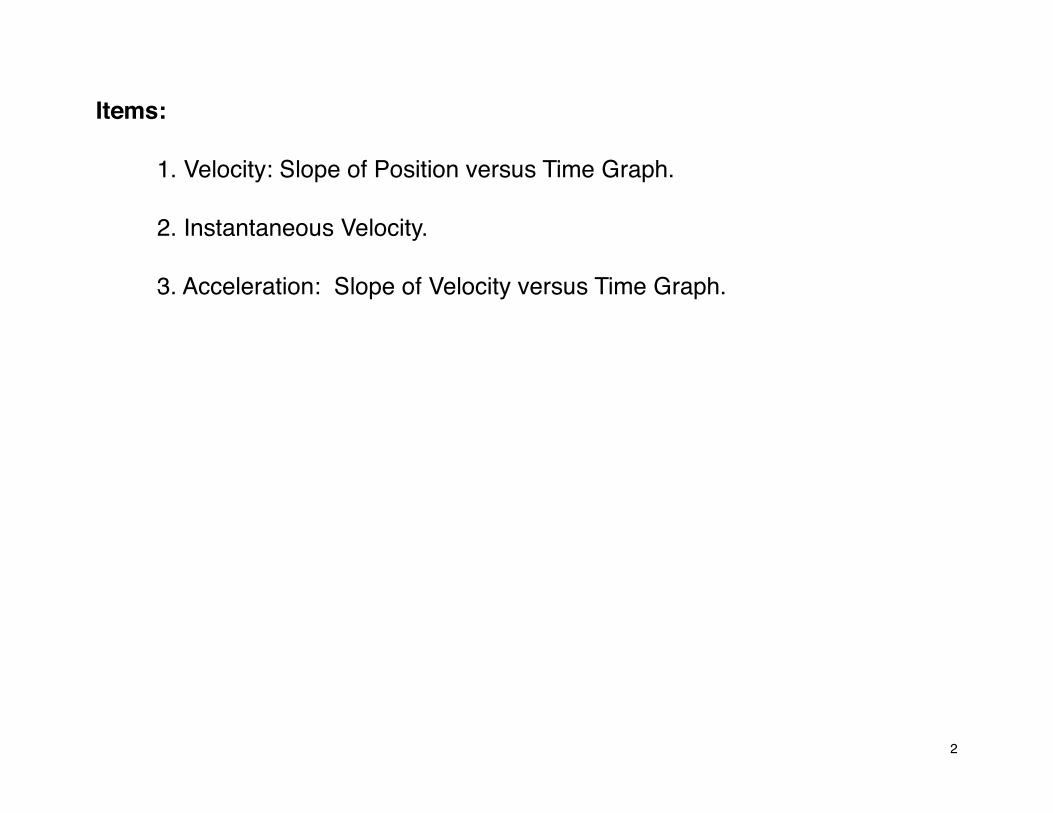
Items:

1. Velocity: Slope of Position versus Time Graph.

2. Instantaneous Velocity.

3. Acceleration: Slope of Velocity versus Time Graph.

2

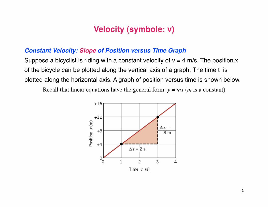
Velocity (symbole: v)

Constant Velocity: Slope of Position versus Time GraphSuppose a bicyclist is riding with a constant velocity of v = 4 m/s. The position x of the bicycle can be plotted along the vertical axis of a graph. The time t is plotted along the horizontal axis. A graph of position versus time is shown below.

Recall that linear equations have the general form: y = mx (m is a constant)

3

Since the position of the bike increases by 4 m every second, the graph of x versus t is a straight line. Furthermore, if the bike is assumed to be at x = 0 m when t = 0 s, the straight line passes through the origin. Each point on this line gives the position of the bike at a particular time. For instance, at t = 1s the position is 4 m, while at t = 3 s the position is 12 m.

The velocity could be determined by considering what happens to the bike between the times of 1s and 3 s, for instance. It is the slope of the line.

4

Calculation: Between the time, 1s (initial) and 3 s (final), the change in time is Δt = (t final - t initial) = (3-1) = 2 s.

During this time interval, the position of the bike changes from + 4 m (initial) to + 12 m (final). So, the change of position Δx = final position - initial position = (x

final - x initial ) = (12 - 4) = 8 m.

The ratio Δx /Δt is called the slope of the straight line and it is the velocity.

Velocity = Slope = Δx /Δt

5

Calculating Velocity from a position-time graph.

• Thus, for an object moving with a constant velocity, the slope of the straight line in a position– time graph gives the velocity. The position (x) is plotted along the vertical axis of a graph. The time (t) is plotted along the horizontal axis.

• Since the position– time graph is a straight line, any time interval t can be chosen to calculate the velocity. Choosing a different t will yield a different x, but the velocity Δx /Δt will not change.

Calculating velocity using a position-time graph

Velocity (v) = slope (x vs t)= Δx /Δt =

change in position / change in time =(x final - x initial ) / (t final - t initial)

6

Example 1: A Bicyclist Riding with a Constant Velocity

In the real world, objects rarely move with a constant velocity at all times, as illustrated in the position versus time graph of a bicycle trip shown below.

7

Analysis of the Graph

Segment 1: Positive velocity: A bicyclist maintains a constant positive velocity on the outgoing leg of a trip. When time increases from 0 s to 600 s, the distance increases from 0 m to 1200 m.

Segment 2: Zero velocity. He maintains zero velocity while stopped. When time increases from 600 s to 1000 s, the distance stays the same at 1200 m (no movement).

Segment 3: Negative velocity. Another constant velocity on the way back. When time increases after 1000 s, the distance decreases from 1200 m and less.

Using the time and position intervals indicated in the drawing, obtain the velocities for each segment ( 1, 2 and 3 ) of the trip.

8

Answer We know that velocity is the slope to the position-time graph. We need to calculate the slope of each segment. velocity = slope = Δx /Δt.

We can take any two points on each segment and find the slope. Usually, we choose the clear points that make the calculation easier.

9

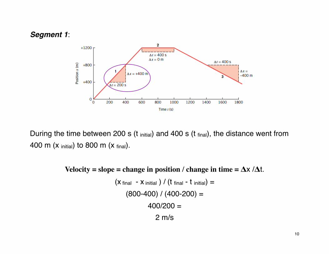
Segment 1:

During the time between 200 s (t initial) and 400 s (t final), the distance went from 400 m (x initial) to 800 m (x final).

Velocity = slope = change in position / change in time = Δx /Δt.(x final - x initial ) / (t final - t initial) =

(800-400) / (400-200) =400/200 =

2 m/s

10

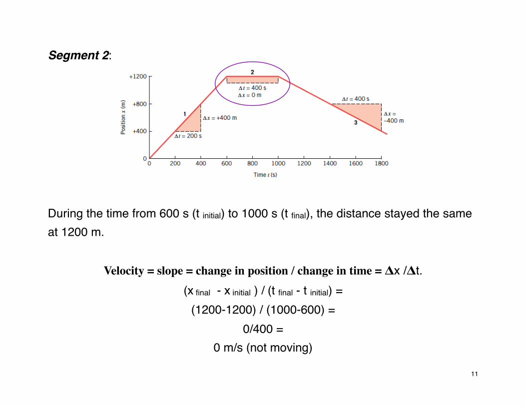
Segment 2:

During the time from 600 s (t initial) to 1000 s (t final), the distance stayed the same at 1200 m.

Velocity = slope = change in position / change in time = Δx /Δt.(x final - x initial ) / (t final - t initial) =

(1200-1200) / (1000-600) =0/400 =

0 m/s (not moving)

11

Segment 3:

During the time from 1400 s (t initial) to 1800 s (t final), the distance changed from 800 m (x initial) to 400 m (x final). He is going back toward initial position.

Velocity = slope = change in position / change in time = Δx /Δt.(x final - x initial ) / (t final - t initial) =

(400- 800) / (1800-1400) =-400/ 400 =

-1 m/s (negative velocity)

12

Summary

13

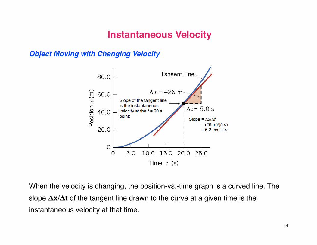
Instantaneous Velocity

Object Moving with Changing Velocity

When the velocity is changing, the position-vs.-time graph is a curved line. The slope Δx/Δt of the tangent line drawn to the curve at a given time is the instantaneous velocity at that time.

14

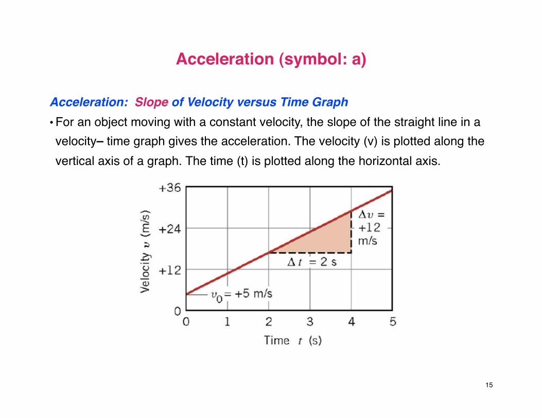
Acceleration (symbol: a)

Acceleration: Slope of Velocity versus Time Graph • For an object moving with a constant velocity, the slope of the straight line in a velocity– time graph gives the acceleration. The velocity (v) is plotted along the vertical axis of a graph. The time (t) is plotted along the horizontal axis.

15

• Since the velocity– time graph is a straight line, any time interval t can be chosen to calculate the acceleration. Choosing a different t will yield a different v, but the velocity Δv /Δt will not change.

Calculating acceleration using a velocity-time graph

Acceleration (a) = slope (v vs t) = Δv /Δt =

change in velocity / change in time =(v final - v initial ) / (t final - t initial)

16

Example 2: An object moving at constant acceleration.

This is the velocity versus time graph of an object moving at constant acceleration. The graph is a straight line (red color). The initial velocity is v0 = 5 m/s when t = 0 s. Calculate the acceleration of this object.

To calculate the acceleration, we need to calculate the slope of the line. We can take the time interval between 2 s (initial ) and 4 s (final). At t = 2 s, the velocity (v initial) is 16 m/s. At t = 4 s, the velocity ( v final) is 28 m/s.

17

Calculation:

Acceleration = slope = change in velocity / change in time = Δv /Δt =

(v final - v initial ) / (t final - t initial) =(28 - 16)/ (4 - 2)=

12 / 2 = 6 m/s2

18

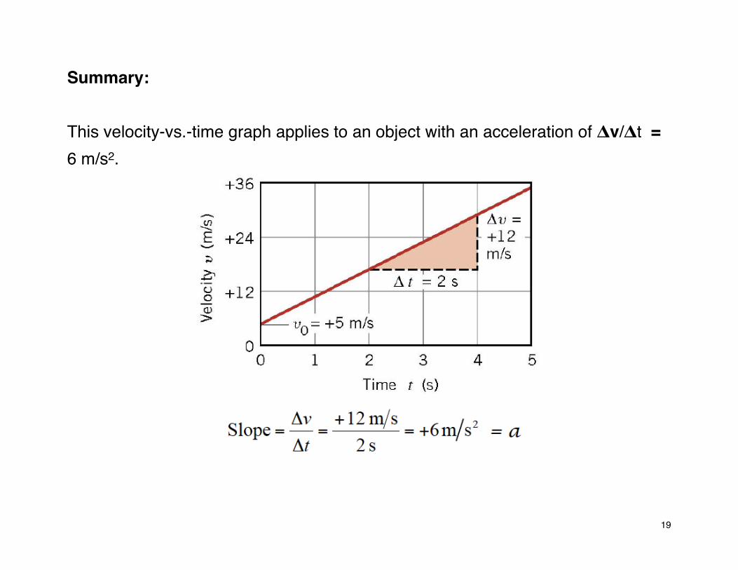
Summary:

This velocity-vs.-time graph applies to an object with an acceleration of Δv/Δt = 6 m/s2.

19

Example 3:

20

References:

1) Humanic. (2013). www.physics.ohio-state.edu/~humanic/. In Thomas Humanic

Brochure Page.

Physics 1200 Lecture Slides: Dr. Thomas Humanic, Professor of Physics, Ohio State

University, 2013-2014 and Current. www.physics.ohio-state.edu/~humanic/

2) Cutnell, J. D. & Johnson, K. W. (1998). Cutnell & Johnson Physics, Fourth Edition.

New York: John Wiley & Sons, Inc.

The edition was dedicated to the memory of Stella Kupferberg, Director of the Photo

Department:“We miss you, Stella, and shall always remember that a well-chosen

photograph should speak for itself, without the need for a lengthy explanation”

21

3) Martindale, D. G. & Heath, R. W. & Konrad, W. W. & Macnaughton, R. R. & Carle,

M. A. (1992). Heath Physics. Lexington: D.C. Heath and Company

4) Zitzewitz, P. W. (1999). Glencoe Physics Principles and Problems. New York:

McGraw-Hill Companies, Inc.

5) Nada H. Saab (Saab-Ismail), ( 2010-2013) Westwood Cyber High School, Physics.

6) Nada H. Saab (Saab-Ismail), (2009- 2014) Wayne RESA, Bilingual Department.

22