19th International Workshop on Unification
143
Laboratoire LOrrain de Recherche en Informatique et ses Applications UMR 7503 Proceedings of the 19th International Workshop on Unification Nara, Japan, April 22, 2005 Edited by Laurent Vigneron (LORIA – UN2-CNRS) LORIA A05-R-022 LORIA, Campus Scientifique, B.P. 239, 54506 Vandœuvre-l` es-Nancy cedex, FRANCE
Transcript of 19th International Workshop on Unification

Laboratoire
LOrrain de
Recherche en
Informatique et ses
Applications
UMR 7503
Proceedings of the
19th International Workshop
on Unification
Nara, Japan, April 22, 2005
Edited by Laurent Vigneron (LORIA – UN2-CNRS)
LORIA A05-R-022
LORIA, Campus Scientifique, B.P. 239, 54506 Vandœuvre-les-Nancy cedex, FRANCE

II

Preface
UNIF is the main international meeting on unification. Unification is concernedwith the problem of identifying given terms, either syntactically or modulo agiven logical theory. Syntactic unification is the basic operation of most au-tomated reasoning systems, and unification modulo theories can be used, forinstance, to build in special equational theories into theorem provers.
The aim of UNIF’2005, as for the eighteen previous meetings, is to bringtogether people interested in unification, present recent (even ongoing) work,and discuss new ideas and trends in unification and related fields. This includesscientific presentations, but also descriptions of applications and softwares usingunification as a strong component.
This workshop is the nineteenth in the series: UNIF’87 (Val d’Ajol, France),UNIF’88 (Val d’Ajol, France), UNIF’89 (Lambrecht, Germany), UNIF’90 (Leeds,England), UNIF’91 (Barbizon, France), UNIF’92 (Dagstuhl, Germany), UNIF’93(Boston, USA), UNIF’94 (Val d’Ajol, France), UNIF’95 (Sitges, Spain), UNIF’96(Herrsching, Germany), UNIF’97 (Orleans, France), UNIF’98 (Rome, Italy),UNIF’99 (Frankfurt, Germany), UNIF’00 (Pittsburgh, USA), UNIF’01 (Siena,Italy), UNIF’02 (Copenhagen, Denmark), UNIF’03 (Valencia, Spain), UNIF’04(Cork, Ireland). For more information on the series:
http://www.lsv.ens-cachan.fr/~treinen/unif/
The UNIF’2005 meeting includes one invited talk, by Joachim Niehren, anda selection of 8 contributed talks.It also includes a panel entitled 20 Years After OBJ2 organized by KokichiFutatsugi (JAIST), with Joseph Goguen (University of California at San Diego),Jean-Pierre Jouannaud (Ecole Polytechnique) and Jose Meseguer (Universityof Illinois at Urbana-Champaign) as additional panelists.
Laurent VigneronUNIF’2005 Organization Chair
April 2005
III

Organization
UNIF’2005 is organized as part of the Federated Conference on Rewriting, De-duction, and Programming (RDP), collocated with RTA (International Con-ference on Rewriting Techniques and Applications) and TLCA (InternationalConference on Typed Lambda Calculi and Applications), and several other af-filiated workshops.
Organization Committee
Philippe de Groote LORIA – INRIA LorraineJoseph Goguen University of California at San DiegoYuichi Kaji Nara Institute of Science and TechnologyPawel Urzyczyn Warsaw UniversityLaurent Vigneron LORIA – UN2-CNRS
Local Organization
Hitoshi Ohsaki National Institute of Advanced Industrial Sci-ence and Technology (AIST)
Masahito Hasegawa Research Institute for Mathematical Sciences,Kyoto University
Cover Design
Maki Ishida National Institute of Advanced Industrial Sci-ence and Technology (AIST)
RDP Sponsors
Nara Convention BureauJSPS International
meeting series
Information Processing Societyof Japan Kansai Branch
TheTelecommunications
AdvancementFoundation
(TAF)Kayamori Foundation of
Infomational ScienceAdvancement
Foundation for Nara Instituteof Science and Technology
IV

Table of Contents
Invited paper
Querying XML-Trees by Tree Automata . . . . . . . . . . . . . . . . . . . . . . . . . . . . 1Joachim Niehren, Laurent Planque, Jean-Marc Talbot, Sophie Tison
Selected papers
Unification with Expansion Variables: Preliminary Results andProblems . . . . . . . . . . . . . . . . . . . . . . . . . . . . . . . . . . . . . . . . . . . . . . . . . . . . . . . 25Adam Bakewell, Assaf J. Kfoury
R-Unification thanks to Synchronized Context-Free Tree Languages . . . . 41Pierre Rety, Jacques Chabin, Jing Chen
Symbolic Debugging in Polynomial Time . . . . . . . . . . . . . . . . . . . . . . . . . . . . 47Christopher Lynch, Barbara Morawska
Combining Intruder Theories . . . . . . . . . . . . . . . . . . . . . . . . . . . . . . . . . . . . . . 63Yannick Chevalier, Michael Rusinowitch
Can Context Sequence Matching Be Used for XML Querying? . . . . . . . . . 77Temur Kutsia, Mircea Marin
Tree vs Dag Automata . . . . . . . . . . . . . . . . . . . . . . . . . . . . . . . . . . . . . . . . . . . 93Siva Anantharaman, Paliath Narendran, Michael Rusinowitch
Relating Nominal and Higher-Order Pattern Unification . . . . . . . . . . . . . . 105James Cheney
Efficiently Computable Classes of Second Order Predicate SchemaMatching Problems . . . . . . . . . . . . . . . . . . . . . . . . . . . . . . . . . . . . . . . . . . . . . . 121Masateru Harao, Shuping Yin, Keizo Yamada, Kouichi Hirata
Panel Discussion
20 Years After OBJ2 . . . . . . . . . . . . . . . . . . . . . . . . . . . . . . . . . . . . . . . . . . . . . 135Organized by Kokichi Futatsugi
Author Index . . . . . . . . . . . . . . . . . . . . . . . . . . . . . . . . . . . . . . . . . . . . . . . . . 137
V

VI

Querying XML-Trees by Tree Automata⋆
Joachim Niehren, Laurent Planque, Jean-Marc Talbot, and Sophie Tison
INRIA Future, Mostrare project, LIFL, Lille, Francehttp://www.grappa.univ-lille3.fr/mostrare
Abstract. Information extraction from semi-structured documents requires tofind n-ary queries in XML trees that define appropriate sets of n-tuples of nodes.In the first part of the talk, we discuss formalism by which to represent monadicqueries in XML trees. In the second part, we report more recent workn on n-ary queries. We propose new representation formalisms by tree automata thatcapture MSO. We then investigate n-ary queries by unambiguous tree automatawhich are relevant for query induction in multi-slot information extraction. Weshow that this representation formalism captures the class of n-ary queries thatare finite unions of Cartesian closed queries, a property we prove decidable.
Keyworks: Semi-structured documents, multi-slot information extraction, XMLquery, tree logic and automata.
1 Introduction
The problem of selecting nodes in trees is the most widespread database query-ing problem in the context of XML [13]. Many applications, however, are facedwith the more general problem of selecting tuples of nodes in trees. We thereforestudy n-ary queries in trees which define sets of n-tuples of nodes.
We are particularly interested in multi-slot information extraction. A typicalproblem in this class of applications is to extract all pairs of products and pricesfrom a set of XML documents. Such pairs are often expressed by pairs of datavalues in nodes of XML trees. In this case, we can solve the extraction problemby distinguishing an appropriate binary query in XML trees.
Monadic queries in trees received considerable attention in in previous workon node selection. The most popular representation formalism is the W3Cstandard XPATH which is used in many other standards in XML technol-ogy (XQuery [1], XPointer [2], etc). Other path based query languages wereproposed in modal logical PDL style [16].
Monadic Datalog in trees is the logic programming approach for expressingmonadic queries. Gottlob and Koch [13, 12] argue in favour of monadic Datalogfor information extraction from semi-structured documents. Monadic Datalogis advantageous because of its high expressiveness (all monadic MSO queriescan be specified), efficient linear time query answering, and usability in visualwrapper (query) specification. It underlies the Lixto system [3] for Web infor-mation extraction. Lixto indeed supports multi-slot information extraction bycomposing monadic queries for all slots.
Tree automata were proposed in several alternative approaches to representmonadic queries. They have a long tradition in querying which dates back to
⋆ The talk presents results from the paper N-ary Queries by Tree Automata
1

2 J. Niehren, L. Planque, J.-M. Talbot, S. Tison
Thatcher and Wright’s seminal paper in 1968 [23]. More recent represention ap-proaches for queries in XML trees proposed hedge automata [6] forest automata[17], query automata [19], selection automata [11], and stepwise tree automata[8].
In this paper, we investigate representation formalisms for n-ary queries intrees by tree automata. We are interested in the class of all regular n-ary queries– those that can be expressed by MSO formulas with n free variables – sincewe believe that this class provides the appropriate expressiveness for multi-slot information extraction from XML trees. We elaborate the tree automataapproach towards expressing n-ary queries, inspired by previous work of Nevenand Bussche [18] and Berlea and Seidl [4].
Representing n-ary queries in trees by tree automata is advantageous forquery induction from annotated examples [7, 15]. Query induction is importantfor improving visual wrapper induction, as argued by Gottlob et. al. [14]. Re-cent induction methods [9, 7, 15], however, remain limited to monadic queriesin trees. As a first step towards remedying this deficiency we present new rep-resentation formalisms for n-ary queries by tree automata.
Contributions of the paper.
1. We propose to represent n-ary queries in ranked trees by successful runs oftree automata.
(a) The class of representable queries are precisely the class of regular queries,i.e., those expressible in MSO.
(b) We show that universal and existential run-based queries have the sameexpressiveness.
2. We investigate the querying power of unambiguous tree automata.
(a) We show that run-based queries with unambiguous tree automata cap-ture the class of regular n-ary queries that are finite unions of someCartesian closed queries.
(b) We show that it is decidable whether a regular n-ary query can be ex-pressed by an unambiguous automaton.
(c) We show that the problem of answering n-ary queries by unambigousautomata on trees has linear time combined complexity.
3. We transfer all results above to n-ary run-based queries in unranked trees –as in XML – with respect to hedge automata [6] and stepwise tree automata[8].
Contribution 1a is new for n-ary queries, but was known in the monadic case[19, 11, 22]. Neven and Bussche’s RAG n-ary queries [18] are more expressivethan MSO and thus run-based n-ary queries. Binary queries by forest automata[4] have not yet been related to MSO.
Result 1b might come as a surprise for n-ary queries, even though it iswell known for monadic queries [18, 5, 11]. It follows by a new proof methodthat does not depend on the two phase query answering algorithm (which iswell-known for monadic queries by attribute grammars, monadic Datalog, orselection automata (see e.g. [18]).

Querying XML-Trees by Tree Automata 3
In the monadic case the characterization means that all regular monadicqueries in tree can be expressed by unambiguous tree automata. This was provedbefore, by Neven and Bussche [18] in the framework of attribute grammars(see IBAGs), by Bloem and Engelfriet [5] in the context of MSO definabletransformations, and a third time for selection automata [11]. Our proof for thegeneral case is original, even for the monadic case. It relies on a correspondencesbetween queries in trees and tree languages that we elaborate, rather than onthe equivalence of tree automata and MSO.
Result 2b implies that it is decidable whether an n-ary query can be ex-pressed a finite union of Cartesian closed queries. The proof 2b is non-trivial.It relies on the decidability of bounded ambiguity in tree automata [21].
Contribution 2c is obtained by generalizing the two phase query answeringalgorithm to the n-ary case.
Our results are highly relevant to a recent approach to query induction [7].This approach induces monadic queries for XML trees that are expressed byruns of unambiguous tree automata. The algorithm extends without change torun-based n-ary queries (1a and 3). The important unambiguity assumption,however, limits its coverage to finite unions of Cartesian closed queries (2a).These can be answered efficiently (2c).
2 Regular queries
We recall the definition of n-ary queries in trees and propose to look at themas tree languages, so that we can define regular n-ary queries by tree automataand relate them to MSO.
2.1 N-ary queries in trees
To keep things as simple as possible, we develop our theory for binary treesrather than for more general ranked trees. Binary trees will prove sufficient toextend all our results to unranked trees (Section 6).
A signature Σ for binary trees fixes a finite set of binary function symbolsf, g and constants a, b. A binary tree t ∈ TΣ is a ground term over Σ:
t ::= a | f(t1, t2)
We define a node of a tree t by its relative address from the root. More formally,we define a function nodes : TΣ → 21,2∗ by structural induction:
nodes(a) = ǫnodes(f(t1, t2)) = ǫ ∪ iπ | 1 ≤ i ≤ 2, π ∈ nodes(ti)
The root of a tree t is the node ǫ. If π1 ∈ nodes(t) then we call π1 first child ofπ and π2 its second child. A leaf is a node without children. An inner node isa node that is not a leaf. For convenience, we will freely identify trees t over Σwith labeling functions of type nodes(t)→ Σ:
a(ǫ) = a,f(t1, t2)(ǫ) = f,f(t1, t2)(iπ) = ti(π) 1 ≤ i ≤ 2, π ∈ nodes(ti)

4 J. Niehren, L. Planque, J.-M. Talbot, S. Tison
In this section, we will study queries for the class of binary trees TΣ with somefixed signature Σ. Our definition of queries, however, will equally apply to otherclasses of trees or graphs that comes with a notion of nodes.
Definition 1. Let n ∈ N and tree a class of trees. An n-ary query for this classis a function q that maps trees t ∈ tree to sets of n-tuples of nodes in t:
∀t ∈ tree : q(t) ⊆ nodes(t)n
Simple examples for monadic queries in binary trees over Σ are the functionsleaf and root that maps trees t to the sets of their leaves resp. to the singletonǫ. The monadic queries labelc for symbols c ∈ Σ map trees t to the set ofc-labeled nodes π of t:
π ∈ labelc(t) iff t(π) = c
The binary query first child relates inner nodes to their first child, while last childlinks inner nodes to their last and thus second child.
Our definition of n-ary queries is quite general in that it does not excludenon-regular queries. For instance, we can query for all pairs (π, π′) in trees tsuch that the subtrees of t on below of π and π′ are equal. This query canindeed be expressed by the RAG’s of Neven and Bussche [18].
In order to formalize what we mean by regular or irregular queries, we willrelate n-ary queries to tree languages (Section 2.2) so that the regularity notionfor tree languages carries over (Section 2.3).
2.2 Canonical tree languages of queries
We will discuss canonical tree languages corresponding to n-ary queries in trees,which are inspired by early work on tree automata and MSO [23, 10]. In Sec-tion 3.2, we will discuss more compact language encodings of queries, that areparticularly useful for query induction.
Let B = 0, 1 be the set of Boolean. We want to encode n-ary queries overΣ as tree languages over the extended signature Σ × Bn. In order to expressan n-ary query q, the canonical approach is to encode all valid membershipstatements (π1, . . . , πn) ∈ q(t) into individual trees over Σ×Bn, so that we cancollect all of them in a tree language. The coding idea is to annotate all nodesπ of tree t by bit vectors (b1, . . . , bn) so that the i-th bit bi is true if and only ifπi = π for all 1 ≤ i ≤ n:
bi ↔ πi = π
For instance, a subset of trees in the canonical tree language of the query childis displayed in Figure 1. We cannot display all of them since that canonicallanguage is infinite.
Let us formally define the correspondence between queries and canonicaltree languages. This requires two concepts: characteristic functions and functionproducts. Let S be a set. For every s ∈ S we define a characteristic functioncs : S → B so that cs(s
′) ↔ s = s′ for all s′ ∈ S. For every tree t andπ ∈ nodes(t) let
cπ : nodes(t)→ B

Querying XML-Trees by Tree Automata 5
Fig. 1. Some of the trees in the canonical tree language of the binary query child
be the characteristic function of π with respect to nodes(t). Characteristic func-tion cπ can be identified with a Boolean trees; these have the same nodes ast. Note that Booleans are overloaded in Boolean trees; they serve as binaryfunction symbols and as constants.
We define the product of m functions fi : A → Bi to be the functionf1 ∗ . . . ∗ fm : A→ B1 × . . .×Bm that satisfies for all a ∈ A:
(f1 ∗ . . . ∗ fm)(a) = (f1(a), . . . , fm(a))
Thereby, we have defined the products of m trees t1, . . . , tm of the same shapebut with possibly distinct signatures Σ1, . . ., Σm, since we identify trees withlabeling functions:
t1 ∗ . . . ∗ tm where ti ∈ TΣifor 1 ≤ i ≤ m
We call a tree t over TΣ×Bn canonical if for all 1 ≤ i ≤ n there exists pre-cisely one node π ∈ nodes(t) such that the i-th Boolean bi = 1 where t(π) =(f, b1, . . . , bn) for some f ∈ Σ. We call a tree language canonical if all its treesare canonical. We write Cann
Σ for the set of all canonical trees over Σ × Bn.
We can now define canonical languages can(q) that correspond to n-aryqueries q over Σ. The trees in can(q) ⊆ TΣ×Bn correspond one-to-one and ontoto the tuples that q selects in trees t ∈ TΣ. Each tree in the canonical languageof q is obtained by multiplying the characteristic functions of some selectednode tuple:
can(q) = t ∗ cπ1 ∗ . . . ∗ cπn | t ∈ TΣ , (π1, . . . , πn) ∈ q(t)
Lemma 1. A tree language L ⊆ TΣ×Bn is canonical if and only if L = can(q)for some n-ary query q over Σ; this query q is always unique.
We next define set operations on n-ary queries over the same signature Σand show that they correspond precisely to the set operations on their canonicaltree languages. This is why we consider canonical languages to be canonical.Given two n-ary queries q1 and q2 we define their union q1 ∪ q2 by imposing forall t ∈ TΣ :
(q1 ∪ q2)(t) = q1(t) ∪ q2(t)
The complement qc of an n-ary query q is the n-ary query satisfying:
qc(t) = nodes(t)n − q(t)

6 J. Niehren, L. Planque, J.-M. Talbot, S. Tison
runsA(a) = p | a→p ∈ rules(A)
r1 ∈ runsA(t1) r2 ∈ runsA(t2) f(r1(ǫ), r2(ǫ))→p ∈ rules(A)
p(r1, r2) ∈ runsA(f(t1, t2))
Fig. 2. Runs of a tree automaton A
The Cartesian product of an n-ary query q1 and an m-ary query q2 is the n+mary query q1 × q2 such that for all trees t ∈ TΣ :
(q1 × q2)(t) = q1(t)× q2(t)
Lemma 2. For all n-ary queries q, q1, q2 and m-ary queries q′ over Σ:
can(q1 ∪ q2) = can(q1) ∪ can(q2)can(qc) = Cann
Σ − can(q)can(q × q′) = t ∗ β ∗ β′ | t ∈ TΣ, t ∗ β ∈ can(q), t ∗ β′ ∈ can(q′)
2.3 Regularity
We recall the definitions of tree automata and regular tree languages and definethe regularity of n-ary queries in trees.
A tree automaton A for binary trees over Σ consists of a finite set states(A),a finite set rules(A), and a set final(A) ⊆ states(A). The rules of A may havetwo forms:
a→ p or f(p1, p2)→ p
where f ∈ Σ is a binary function symbol, a ∈ Σ a constant and p, p1, p2 ∈states(A).
A run of a tree automata A on a tree t is a function r : nodes(t)→ states(A)that associates states to nodes of t according to the rules of A, or equivalently,a tree labeled in states(A) with the same domain than t. Figure 2 defines theset runsA(t) of runs of A on t by recursion on the structure of t.
A run r of a tree automaton A on a tree t is called successful if it labels theroot of t by some state in final(A).
succ runsA(t) = r ∈ runsA(t) | r(ǫ) ∈ final(A)
Example 1. Consider automaton A1 over signature Σ = f, a. Two runs of A1
are presented in Figure 3. Successful runs of A1 on arbitrary trees label the leftmost a-leaf by 1 and all others by ∗. The ancestors of the left most a-leaf willbe assigned to y. All other inner nodes will be marked by ∗. The final statesare y and 1. In summary, we have the following states:
states(A1) = 1, ∗, yfinal(A1) = 1, y
The rules in rules(A1) need to verify the intuitive meaning that we associatedwith the states:
a→ 1 f(1, ∗)→ y f(y, ∗)→ ya→ ∗ f(∗, ∗)→ ∗

Querying XML-Trees by Tree Automata 7
f, y
f, y a, ∗
a, 1 a, ∗
f, ∗
f, ∗ a, ∗
a, ∗ a, ∗
Fig. 3. Two runs of automaton A1 on the same tree; only the left one is successful.
Note that every tree permits at most one successful run by automaton A1 butpossibly other unsuccessful runs.
A tree t is accepted by a tree automaton A if A has a successful run on t, i.e.,succ runsA(t) 6= ∅. The language L(A) recognized by a tree automaton A is theset of trees t that A accepts. A tree language L ⊆ TΣ is regular if and only if itis recognized by some tree automaton A over Σ, so that L = L(A). AutomatonA1 from Example 1, for instance, accepts all trees in Tf,a.
Definition 2. A n-ary query q in trees over Σ is regular if its canonical treelanguage can(q) ⊆ TΣ×Bn is recognized by a tree automaton.
Proposition 1. Regular queries are closed under union, intersection, comple-mentation, and Cartesian products.
Proof. This follows from Lemma 2. To see this, let us exemplify the proof for theunion operator. If q1 and q2 are regular queries then by definition their canonicallanguages are regular: can(q1) and can(q2). Unions of regular tree languages areregular, and thus can(q1) ∪ can(q2). This language is equal to can(q1 ∪ q2) byLemma 2. The regularity of can(q1 ∪ q2) is equivalent to that q1 ∪ q2 is regularby definition.
Let us recall three standard notions for tree automata: determinism, unambi-guity, and relabelings [10]. A tree automaton A is (bottom-up) deterministic ifno two of its rules have the same left hand side. It is unambiguous, if no treet ∈ TΣ permits more than one successful run in succ runsA(t).
A relabeling morphism for binary signatures Σ and Σ′ is a mapping h :Σ → Σ′ that maps constants to constants and binary function symbols tobinary function symbols. Relabeling morphisms h : Σ → Σ′ can be lifted ho-momorphically to trees h : TΣ → TΣ′ by imposing for all f ∈ Σ and t, t′ ∈ TΣ :
h(f(t1, t2)) = h(f)(h(t1), h(t2))
It is well-known that relabeling morphisms as well their inverse images preserveregularity, i.e. if L ⊆ TΣ is regular then h(L) and if L′ ⊆ TΣ′ is regular thenh−1(L′).
2.4 MSO queries
We recall the monadic second-order logic (MSO) in binary trees and how itcan be used to represent n-ary queries. The classical theorem of Thatcher and

8 J. Niehren, L. Planque, J.-M. Talbot, S. Tison
Wright [23] then shows that regular n-ary queries capture precisely the class ofMSO definable n-ary queries.
We identify binary trees t ∈ TΣ with logical structures. The domain of thestructure of t is the set nodes(t). Its signature consists of the binary relationsymbols first child and last child, and the monadic relation symbols labela for alla ∈ Σ. These symbols are interpreted by the corresponding node relations of t.
first childt = (π, π1) | π1 ∈ nodes(t)last childt = (π, π2) | π2 ∈ nodes(t)
labelta = π | t(π) = a
Let x, y, z range over an infinite set of node variables and p over an infinite setof monadic predicates. Formulas φ of MSO have the following abstract syntax:
φ ::= p(x) | first child(x, y) | last child(x, y) | labela(x)| ¬φ | φ1 ∧ φ2 | ∀x.φ | ∀p.φ
A variable assignment α into a tree t maps node variables to nodes of t andmonadic predicates to sets of nodes of t. We define the validity of formulas φin trees t under variable assignments α in the usual Tarskian manner:
t, α |= φ
Formulas φ with n free variables x1, ..., xn represent n-ary queries queryφ(x1,...,xn)
which satisfies for all trees t ∈ TΣ
queryφ(x1,...,xn)(t) = (α(x1), ..., α(xn)) | t, α |= φ
Theorem 1. (Thatcher and Wright [23]): An n-ary query in binary trees isregular if and only if it can be expressed by some MSO formula with n free nodevariables.
3 Run-based queries
We now introduce new representation formalisms for regular n-ary queries basedon successful runs of tree automata, that conservatively extend previous ap-proaches to monadic queries [18, 11, 22]. Run-based query formalisms are strictlyless expressive that Neven and Bussche’s [18] n-ary relational attribute gram-mars (RAGs) queries, and technically simpler. They provide a simpler and moregeneral alternative to Seidl and Berlea’s [4] binary queries in unranked trees byforest automata.
3.1 Existential run-based queries
The idea is to use successful runs of tree automata not only to accept trees butalso to select nodes in them. This way, one can avoid the indirection through cor-responding tree languages in representations formalism. As we will see, this cor-respondence will reappear when proving that run-based queries capture MSO.
Querying XML-Trees by Tree Automata 9
A run-based n-ary query in binary trees over Σ is specified by a tree au-tomaton A over Σ and a set S ⊆ states(A)n of so called selection tuples. Anexistential run-based query query∃A,S selects all those tuples of nodes (π1, . . . , πn)in a tree t that are assigned to a selection tuple by some successful run of A ont:
query∃A,S(t) = (π1, . . . , πn) | ∃r ∈ succ runsA(t), (r(π1), . . . , r(πn)) ∈ S
Example 2. Reconsider automaton A1 from Example 1. The monadic queryqueryA1,1 selects the left most a-leaf.
This monadic query cannot be represented by any deterministic tree au-tomaton. Non-determinism is needed to distinguish different occurrences of a-leaves. Automata have to guess states for nodes when processing trees bottomup. The guesses need be checked for correctness: they are correct only if theycan be extended to a successful runs.
Example 2 illustrates that runs of deterministic tree automata are not suf-ficient to define all regular monadic queries (even though they can recognizeall regular languages). Nevertheless, one can do with a limited form of non-determinism in monadic queries. Unambiguous automata are enough, as in theexample. This means that there exists always exists at most one correct wayof guessing states. This result is well know in the monadic case. It was provedin the context of attribute grammars by Neven and Bussche [18] and indepen-dently by Bloem and Engelfriet [5].
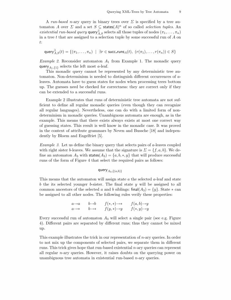
Example 3. Let us define the binary query that selects pairs of a-leaves coupledwith right sister b-leaves. We assume that the signature is Σ = f, a, b. We de-fine an automaton A3 with states(A3) = a, b, ∗, y that will produce successfulruns of the form of Figure 4 that select the required pairs as follows:
queryA3,(a,b)
This means that the automaton will assign state a the selected a-leaf and stateb the its selected younger b-sister. The final state y will be assigned to allcommon ancestors of the selected a and b siblings: final(A3) = y. State ∗ canbe assigned to all other nodes. The following rules verify these properties:
a→a b→b f(∗, ∗)→∗ f(a, b)→ya→∗ b→∗ f(y, ∗)→y f(∗, y)→y
Every successful run of automaton A3 will select a single pair (see e.g. Figure4). Different pairs are separated by different runs; thus they cannot be mixedup.
This example illustrates the trick in our representation of n-ary queries. In orderto not mix up the components of selected pairs, we separate them in differentruns. This trick gives hope that run-based existential n-ary queries can representall regular n-ary queries. However, it raises doubts on the querying power onunambiguous tree automata in existential run-based n-ary queries.

10 J. Niehren, L. Planque, J.-M. Talbot, S. Tison
f,y
f,y
a,a b,b
f,*
a,* b,*
f,y
f,*
a,* b,*
f,y
a,a b,b
Fig. 4. The two successful runs select both pairs of a-leaves and right sister b-leaves
f,y
f,y
a,a b,b
a,a
⇒ f,0,0
f,0,0
f,1,0 f,0,1
f,1,0
Fig. 5. From runs to Boolean query representations: select pairs of a-leaves and b-leaves
3.2 Compact tree languages for queries
Runs of tree automata can select a whole set of tuples. Sets of runs thus providea much more compact query representations than canonical tree languages. Thisholds in particular for queries by unambiguous tree automata where all tuplesfor a tree are selected in a single run.
Understanding the expressive power of existential run-based queries is bestbased on a correspondence between arbitrary tree languages over Σ × Bn andn-ary queries over Σ. This means that we give up canonicity in favour of com-pactness.
Example 4. Let us select pairs of a-leaves and b-leaves. This query is the Carte-sian product of two monadic queries for a-leaves and b-leaves respectively. Itcan be defined by tree automaton A4 with states(A4) = a, b, y and rules:
a→ a, b→ b, f(p, p′)→ y for all p, p′ ∈ a, b, y
All a-leaves will be mapped to state a, all b-leaves to state b, and all innernodes to state y. All states are final: final(A4) = a, b, y. The query is definedby queryA4,(a,b).
Automaton A4 is deterministic and thus unambiguous. Let t ∈ TΣ andsuppose that r is the unique successful run of A4 on t. The tree t ∗ r can beeasily transformed into a tree over Σ × B2 that compactly encodes all tuplesselected by the automaton on t. An example is illustrated in Figure 5.
The example illustrates that every tree language L ⊆ TΣ×Bn – canonical ornot – corresponds to an n-ary query in trees over Σ. In order to define this queryformally, we need a partial order on bit-vectors in (b′1, . . . , b
′n), (b1, . . . , bn) ∈ Bn:
(b′1, . . . , b′n) ≤ (b1, . . . , bn) iff ∀1 ≤ i ≤ n. b′i ≤ bi
We next lift this partial order to trees whose labels are extended by bit vectorst ∗ β′, t ∗ β ∈ TΣ×Bn :
t ∗ β′ ≤ t ∗ β iff ∀π ∈ nodes(t). β′(π) ≤ β(π)

Querying XML-Trees by Tree Automata 11
Let L ⊆ TΣ×Bn be a tree language. The corresponding n-ary query corr query(L)is the unique query whose canonical tree language satisfies:
can(corr query(L)) = t ∗ β′ ∈ CannΣ | ∃t ∗ β ∈ L. t ∗ β
′ ≤ t ∗ β
Lemma 3. If L ⊆ TΣ×Bn is a regular tree language then the correspondingn-ary query corr query(L) is regular too.
Proof. Let ⊥0 be a constant and ⊥2 be a binary symbol. We define two rela-beling morphism such that for all g ∈ Σ and b, b′ ∈ Bn: JN: Picture needed
Σn,n = Σ × Bn × Bn
h : Σn,n → (Σ × Bn) ∪ ⊥0,⊥2h((g, b, b′)) = if b ≤ b′ then (g, b′) else ⊥arity(g)
h1 : Σn,n → Σ × Bn
h1((g, b, b′)) = (g, b)
We then have can(corr query(L)) = h1(h−1(L))∩Cann
Σ. This language is regularsince L and Cann
Σ are.
3.3 Existential queries and regularity
Our next goal is to show that existential run-based queries capture the class ofregular n-ary queries.
Lemma 4. Existential run-based n-ary query are regular.
Proof. Existential run-based queries are finite unions of existential run-basedqueries with singleton selection sets:
query∃A,S = ∪p∈S query∃A,p
By Proposition 1 it remains to show that run-based queries query∃A,p withsingleton selection sets are regular. Let us fix an automaton A with signatureΣ and selection tuple p = (p1, . . . , pn) ∈ states(A)n. For every p ∈ states(A),let cp : states(A) → B be the characteristic function of p. We construct a newautomaton Ap over the signature Σ×Bn so that for all trees t∗β ∈ TΣ×Bn andfunctions r : nodes(t)→ states(A):
r ∈ succ runsA(t) and β = cp1 r ∗ . . . ∗ cpn riff r ∈ succ runsAp
(t ∗ β)
Both automata have the same runs but on slightly different trees. The idea isthat runs of Ap additionally test whether the bit vectors in tree β are licensedby runs of A on t with respect to the selection tuple p. We define automatonAp such that:
a→p′ ∈ rules(A)
(a, cp1(p′), . . . , cpn(p′))→ p′ ∈ rules(Ap)
f(p′1, p′2)→p
′ ∈ rules(A)
(f, cp1(p′), . . . , cpn(p′))(p′1, p
′2)→p
′ ∈ rules(Ap)

12 J. Niehren, L. Planque, J.-M. Talbot, S. Tison
final(Ap) = final(A)
The query corresponding to L(Ap) is regular by Lemma 3. It remains to verifythat this query is identical to query∃A,p:
corr query(L(Ap)) = query∃A,p
This mainly follows from the definitions of corresponding tree languages andthe above property of Ap. We show for all trees t ∈ TΣ and nodes π1, . . . , πn ∈nodes(t):
(π1, . . . , πn) ∈ corr query(L(Ap))(t)⇔ t ∗ cπ1 ∗ . . . ∗ cπn ∈ can(corr query(L(Ap)))⇔ ∃t ∗ β ∈ L(Ap). t ∗ cπ1 ∗ . . . ∗ cπn ≤ t ∗ β⇔ ∃β∃r ∈ succ runsAp
(t ∗ β). t ∗ cπ1 ∗ . . . ∗ cπn ≤ t ∗ β⇔ ∃r ∈ succ runsA(t). t ∗ cπ1 ∗ . . . ∗ cπn
≤ t ∗ cp1r ∗ . . . ∗ cpnr⇔ ∃r ∈ succ runsA(t). r(π1) = p1, . . . , r(πn) = pn
⇔ (π1, . . . , πn) ∈ query∃A,p(t)
Lemma 5. Every regular n-ary query is equal to some existential run-basedquery.
Proof. Let L be a regular language over Σ×Bn and A be an automaton suchthat L(A) = L. We compute an automaton C over Σ and a selection set S suchthat L(C) = t | t ∗ β ∈ L(A) and corr query(L(A)) = query∃C,S:
(a, b1, ..., bn)→q ∈ rules(A)
a→(q, b1, ..., bn) ∈ rules(C)
(f, b1, ..., bn)(q1, q2)→q ∈ rules(A)
(f(q1, b11, ...b
n1 ), (q2, b
12, ..., b
n2 ))→(q, b1, ..., bn) ∈ rules(C)
Finally, let states(C) = states(A)∗Bn, final(C) = final(A)×Bn and S = Q1 ×...×Qn where for all 1 ≤ i ≤ n:
Qi = (q, b1, ..., bn) ∈ states(C) | bi = 1
The correctness of the construction is proved by showing that for any termt, runsC(t) = β | r ∈ runsA(t ∗ β) and succ runsC(t) = β | r ∈ succ runsA(t ∗β).
Theorem 2. Existential run-based n-ary queries capture precisely the class ofregular n-ary queries.
3.4 Universal run-based queries
Universal run-based query quantify universally over successful runs rather thanexistentially.
query∀A,S(t) = (π1, . . . , πn) | ∀r ∈ succ runsA(t), (r(π1), . . . , r(πn)) ∈ S

Querying XML-Trees by Tree Automata 13
rules(A6) :a→ 0 f(1, 2) → y
a→ 1 f(0, y) → y
a→ 2 f(y, 0) → y
f(0, 0) → 0f(0, 0) → 1f(0, 0) → 2
final(A6) = y, 1, 2
selection tuples:S6 = (1, 2), (0, 0), (y, 0), (0, y)
Fig. 6. An example for a universal run-based query: next sibl = query∀A6,S6= query∃A6,(1,2)
Universal queries were proposed before in selection automata [11] and universalBAGs [18].
An example is given in Figure 6. We represent the binary query next sibluniversally, which relates first and second children with the same mother. Suc-cessful runs of automaton A6 will assign the state pair (1, 2) to at most onenode pair satisfying the query. Descendants and cousins of these nodes will beassigned to state 0, all others (ancestors in fact) to y. The required query canbe expressed existentially by query∃A6,(1,2).
Runs in universal queries refute all those tuples that they don’t select.Thus, one needs sufficiently many selection states so that correct tuples arenever rejected. In the example, selected pairs will always be labeled by statepairs in S6 = (1, 2), (0, 0), (0, y), (y, 0). All other node pairs can be refutedby successful runs that assign state pairs in the complement of S6. Hencequery∃A6,(1,2) = query∀A6,S6
.
Lemma 6. The complement of an existential run-based query is an existentialrun-based query.
Proof. Let q be an existential query. By Lemma 4, q is regular, so can(q) isregular. By Lemma 2, can(qc) = Cann
Σ − can(q). As can(q) ⊆ CannΣ ⊆ TΣ×Bn ,
then can(qc) = CannΣ ∩ canc(q), with canc(q) is the complement of can(q) into
TΣ×Bn . So, can(qc) is regular and by Lemma 5, qc is existential.
Theorem 3. Existential and universal queries have the same expressiveness.
Proof. We prove first that any universal query has an equivalent existentialquery. An universal query can be written as query∀A,S for an automaton A anda set S ⊆ states(A)n.
query∀A,S(t) = π | ∀r ∈ succ runsA(t), r(π) ∈ S
Obviously, the complement of query∀A,S(t) is precisely the set
π | ∃r ∈ succ runsA(t), r(π) ∈ states(t)n\S
This is by definition query∃A,states(t)n\S . We can now conclude using that exis-
tential queries are closed under complement (Lemma 6). We prove now that

14 J. Niehren, L. Planque, J.-M. Talbot, S. Tison
any existential query has an equivalent universal query. By Lemma 6, for anyexistential query q, there exists A and S such that q = (query∃A,S)c. Therefore,for any tree t, q(t) is equal to
π | ∀r ∈ succ runsA(t), r(π) ∈ states(t)n\S
This is precisely query∀A,states(t)n\S
4 Unambiguous tree automata
Our next goal is to investigate the querying power of unambiguous tree au-tomata in the n-ary case. Monadic queries by unambiguous tree automata areused in a recent approach to query induction from annotated examples [7].We believe that this approach can be extended from monadic queries to n-aryqueries. This is why we want to understand the precise expressiveness of n-aryqueries by unambiguous tree automata.
The main idea for query induction in the cite approach to represent n-aryqueries over Σ as tree languages over Σ × Bn and to infer tree automata forsuch tree languages by methods of grammatical inference [20]. Compact treelanguages for representing queries seem advantageous; they are much easier toinfer than canonical tree language. N-ary queries by unambiguous tree automataallow for compact representation, where all tuples selected in a single tree overΣ can be represented by a single tree over Σ × Bn.
4.1 Finite unions of Cartesian closed queries
We call a n-ary query Cartesian closed if it is a Cartesian product of monadicqueries.
Proposition 2. Run-based n-ary queries queryA,S by unambiguous automataA are finite unions of Cartesian closed n-ary queries.
Proof. We show that queryA,S is Cartesian closed for singletons S. Let S =(p1, . . . , pn). As for any tree t there exists at most one successful run r by A,we have:
queryA,S = queryA,p1 × . . .× queryA,pn
Theorem 4. Run-based queries by unambiguous tree automata capture the classof finite unions of Cartesian closed regular queries.
The simple direction is proved by Proposition 2. The converse is more involved;it needs some auxiliary notions.
We define sat(q), the saturated language of q, as the least subset of TΣ×Bn
satisfying (i) can(q) = can(corr query(sat(q))) and (ii) for all t ∈ TΣ , t ∗ βbelongs to sat(q) if either there exists t∗β′ in can(q) such that t∗β′ ≤ t∗β or βsatisfies β(π) = 0n for all π ∈ dom(t). Moreover, we define max(q) the languageof maximals for q defined as t ∗ β ∈ sat(q) | ¬(∃t ∗ β′ ∈ sat(q) : t ∗ β < t ∗ β′).
Lemma 7. Let q be a regular query. Then both sat(q) and max(q) are regularand computable.

Querying XML-Trees by Tree Automata 15
Proof. Let ⊥0 be a constant and ⊥2 be a binary symbol. We define two rela-beling morphisms such that for all g ∈ Σ and b, b′ ∈ Bn:
h′ : Σ × Bn × Bn → (Σ × Bn) ∪ ⊥0,⊥2h′((g, b, b′)) = if b ≤ b′ then (g, b) else ⊥arity(g)
h2 : Σ × Bn × Bn → Σ × Bn
h2((g, b, b′)) = (g, b′)
Let us define up(q) the set h2(h′−1(can(q))). Now, let us consider qc be the
query complement of q and let up(qc) be the set h2(h′−1(can(qc)). Obviously,
one can built automata for up(q) and up(qc). Therefore, one can do so forsat(q) = up(q) − up(qc). Considering now the relabeling morphism h1 definedin proofs of Lemma 3, max(q) can be defined as sat(q)∩ (h1(h
−12 (sat(q))∩SG))c
where SG is the regular language of trees written over the signature Σ×Bn×Bn
such that for any t ∗ β ∗ β′ in SG, it holds that t ∗ β < t ∗ β′.
Proposition 3. Let q be a Cartesian closed n-ary query. For all t ∈ TΣ, thereexists exactly one tree t ∗ β in max(q).
Proof. The query q being Cartesian closed, for all t ∈ TΣ , it can be writtenas Et
1 × . . . × Etn. For each t ∈ TΣ, we consider the tree t ∗ βq defined as
for all π ∈ dom(t) and βq(π) = (b1, . . . , bn), bi ↔ (π ∈ Eti ). Defining Lq as
t ∗ βq | t ∈ TΣ, it is easy to verify q = corr query(Lq).
Proposition 4. Let q be a Cartesian closed regular n-ary query. Then q is aunambiguous query.
Proof. By Lemma 7 we can compute an automaton M recognizing max(q). Wlogwe assume M to be deterministic. By Lemma 5, we can compute some automa-ton C for trees from TΣ such that succ runsC(t) = r∗β | r ∈ succ runsM (t∗β).As M is deterministic, succ runsM (t ∗ β) contains at most one element. More-over, there is a unique β such that t ∗ β is accepted by M for any tree t ∈ TΣ
(by Proposition 3). Therefore, succ runsC(t) is singleton set.
Now cnsider the query q such that there exists Cartesian closed regularqueries q1, . . . , qk verifying for all t ∈ TΣ , q(t) =
⋃kj=1 qj(t). We know by Propo-
sition 4 that for each qj there exists some pair (Aj , Sj) such that qj = queryAj ,Sj
and Aj is unambiguous. The rest of the proof is essentially the computation ofthe product of the Aj’s. But, it must be done carefully to preserve the unam-biguity of the result JN: unambiguity is not the problem, we have to ensureruns of A if there exists runs in some Ai: we consider Ai the deterministicautomaton accepting the trees not accepted by Ai; assuming Ai and Ai havedisjoint sets of states, we define A′
i as Ai∪ Ai. This automaton A′i is unambigu-
ous and moreover, query∃A′i,Si
= query∃Ai,Si. For q, we define the automaton A as
the product of the A′i’s and let final(A) = final(A′
1)× . . .× final(A′k). Note that
A is unambiguous. We define S as the set of all (p1, . . . , pn) ∈ states(A)n forwhich there exists i (1 ≤ i ≤ k) such that (proji(p1), . . . , proji(pn)) ∈ Si (whereproji(p) is the ith component of the state p). The two queries q and query∃A,S
are equivalent. This completes the proof of Theorem 4.

16 J. Niehren, L. Planque, J.-M. Talbot, S. Tison
Proposition 5. A query q is unambiguous iff it can be expressed as Booleancombinations of monadic MSO formulas (i.e., regular monadic queries)
4.2 Deciding unambiguity of queries
We show in this section that one can decide whether a regular n-ary query isunambiguous, or equivalently by Theorem 4 whether the query is a finite unionof Cartesian closed regular queries.
Note that deciding whether a regular query is Cartesian closed is straight-forward using relationship between regular queries and MSO formulas and usingthat the Cartesian closed property is MSO-definable. Considering finite unionsof Cartesian closed regular queries requires more sophisticated technique.
Theorem 5. The problem whether an n-ary regular query is a finite union ofCartesian closed regular queries is decidable.
We say that a tree automaton A is k-ambiguous if for any tree t ∈ TΣ , thereexists at most k accepting runs for t in A. An automaton A has a boundedambiguity if there exists some natural k such that A is k-ambiguous.
Theorem 6. [21] The boundedness of ambiguity is decidable for tree automata.
Proposition 6. For any query q, if there exists some pair (A,S) such thatq = query
∃A,S and A has a bounded ambiguity then q is a finite union of Cartesian
closed queries.
Proof. By definition, we have q(t) =⋃
s∈S qs(t) for any t ∈ TΣ and qs ∈query∃A,s. Now, for any tree t and any accepting run for t in A, we define qs
r(t) as
(π1, . . . , πn) | (r(π1), . . . , r(πn)) = s. Therefore, qs(t) =⋃
r∈succ runsA(t) qsr(t).
As there exists some natural k such that the cardinality of succ runsA(t) issmaller than k for any t, we have indeed that q is a finite union of Cartesianclosed queries.
Proposition 7. For any regular query q, if q is a finite union of Cartesianclosed queries then there exists some natural l such that for all trees t ∈ TΣ,the cardinality of the set t ∗ β | t ∗ β ∈ max(q) is upper-bounded by l.
Proof. The query q being a finite union of Cartesian closed queries, there existssome natural k s.t. q =
⋃kj=1 q
1j × . . . × q
nj , each qi
j being a monadic regularquery.
Let t be a tree from TΣ . For each i, 1 ≤ i ≤ n, we define ≡i, an equiv-alence relation on dom(t) by π ≡i π′ if for all (π1, . . . , πi−1, πi+1, . . . , πn),(π1, . . . , πi−1, π, πi+1, . . . , πn) belongs to q(t) iff (π1, . . . , πi−1, π
′, πi+1, . . . , πn)belongs to q(t). This just means that π and π′ are, in some sense, interchange-able in ith position. Then, let π and π′ be two nodes. If for each j, 1 ≤ j ≤ k,π belongs to qi
j(t) iff π′ belongs to qij(t), then π ≡i π
′. This implies that ≡i
is of finite index bounded by 2k. Now let t ∗ β be a term in max(q). Let πselected in the ith position by β i.e. such that β(π)i = 1. Then, by maximalityof t ∗ β, for each π′ s.t. π ≡i π
′, we have also β(π′)i = 1. This implies thatπ | β(π)i = 1 is an union of equivalence classes for ≡i. So, the cardinality of
the set t ∗ β | t ∗ β ∈ max(q) is upper-bounded by 2n.2k.
Querying XML-Trees by Tree Automata 17
Proposition 8. For any regular query q, if there exists some natural l suchthat for all trees t ∈ TΣ, the cardinality of the set t ∗ β | t ∗ β ∈ max(q) isupper-bounded by l then there exists some k-ambiguous automaton A and someset S of tuples of states such that q = query
∃A,S.
Proof. The proof is similar to that of Proposition 4 and relies on the construc-tion defined in the proof of Lemma 5.
Theorem 5 easily follows from Theorem 6 and Propositions 6, 7 and 8. Moreover,we can show that
Corollary 1. Let q be a regular query. Then the two following statements areequivalent: (1) q is a finite union of Cartesian closed queries. (2) q is a finiteunion of Cartesian closed regular queries.
Proof. Obviously, (2) implies (1). We know by Propositions 6, 7 and 8 that qis a finite union of Cartesian closed queries iff there exists some natural l suchthat for all trees t ∈ TΣ , the cardinality of the set t | t ∗ β ∈ max(q) is upper-bounded by l. So, it suffices to prove that this latter implies that q is a finiteunion of Cartesian closed regular queries. We recall that q being regular, onecan compute the automaton max(q). We define a total strict ordering ≺ on treesfrom TΣ×Bn as follows: t ∗ β ≺ t ∗ β′ if (i) β(ǫ) < β′(ǫ), or (ii) β(ǫ) = β′(ǫ) andt1 ∗β1 ≺ t1 ∗β
′1 or (iii) β(ǫ) = β′(ǫ), t1 ∗β1 = t1 ∗β
′1 and t2 ∗β2 ≺ t2 ∗β
′2 (where
tj ∗βj is the subtree at position j of t∗β). Obviously, ≺ is a recognizable relationof TΣ×Bn × TΣ×Bn . Using ideas similar to those from proof of Lemma 7 we cancompute automata for S1, the set of greatest elements in the sense of ≺ frommax(q) and for R1 as max(q)−S1. Obviously, S1 contains at most one tree t ∗ βfor each t ∈ TΣ . Therefore, the regular query q1 defined as q1(t) = tuples(t ∗ β)for the unique t ∗ β in S1, is a Cartesian closed query. We iterate the sameprocess l times, extracting each time a Cartesian closed regular query qj. It isstraightforward that q is the union of all these qj ’s.
4.3 Construction of unambiguous automata
We next give a direct construction of unambiguous automata for Cartesianclosed run based queries query∃A,S. The idea of the construction is that of thetwo way querying answering algorithm. Note that the existence unambiguousautomata follows already from the more general Theorem 4. The direct con-struction might be of interest nevertheless, if one wants to analyse the size ofresulting unambiguous automaton.
We first compute a deterministic automaton det(A) that can perform allruns of A at once:
states(det(A)) = 2states(A)
final(det(A)) = P | P ∩ final(A) 6= ∅
P = p | a→ p ∈ rules(A)a→ P ∈ rules(det(A))
P = p | f(p1, p2)→ p ∈ rules(A), p1 ∈ P1, p2 ∈ P2
f(P1, P2)→ P ∈ rules(det(A))

18 J. Niehren, L. Planque, J.-M. Talbot, S. Tison
Proposition 9. For every run r ∈ runsdet(A)(t) and node π ∈ nodes(t): r(π) =r′(π) | r′ ∈ runsA(t).
We next compute an unambiguous automaton u(A) that for all trees t computesall successful runs of A on t at once:
states(u(A)) = (P ′, P ) | P ′ ⊆ P,P ∈ states(det(A))
final(u(A)) = (P ∩ final(A), P ) | P ∈ final(det(A))
a→ P ∈ rules(det(A)) P ′ ⊆ P
a→ (P ′, P ) ∈ rules(u(A))
f(P1, P2)→ P ∈ det(A)P ′
1 = p1 ∈ P1 | p2 ∈ P2, p′ ∈ P ′, f(p1, p2)→ p′ ∈ rules(A)
P ′2 = p2 ∈ P2 | p1 ∈ P1, p
′ ∈ P ′, f(p1, p2)→ p′ ∈ rules(A)
f((P ′1, P1), (P
′2, P2))→ (P ′, P ) ∈ rules(u(A))
Proposition 10. For all trees t, automata A, runs r ∈ succ runsu(A)(t), andnodes π ∈ nodes(t):
r(π) = (r′(π) | r′ ∈ succ runsA(t), r′(π) | r′ ∈ runsA(t))
In particular, u(A) is unambiguous.
Theorem 7. Cartesian closed n-ary queries query∃A,S can be expressed by un-
ambiguous tree automata u(A); if Si = pi | (p1, . . . , pn) ∈ S for all 1 ≤ i ≤ nthen:
query∃A,S = query
∃u(A),S1
× . . .× query∃u(A),Sn
5 Query Answering
We next show that we can answer n-ary queries by runs of unambiguous au-tomata in linear time combined complexity. This can be done by extending thewell-known two phase query answering algorithm.
The general problem seems to have a higher computational complexity. Thedata complexity of unrestricted run-based n-ary queries is remains polynomialfor fixed n ≥ 0 but the combined complexity seems to be higher. To see thepolynomial bound on the data complexity, we fix an automaton A over Σ.The inputs are a set of selection tuples S ⊆ nodes(A)n and a tree t ∈ TΣ. Wecompute an automaton A′ from A and S that recognizes the canonical languageof query∃A,S. We then test for all tuples (π1, . . . , πn) ∈ nodes(t)n whether t∗ct
π1∗
. . . ctπ1∈ L(A′). If we assume the size on A to be bounded by some constant then
each of this tests will be in linear time O(|t|). So the overall data complexity isbounded O(|t|)n+1.
Theorem 8. The combined complexity for answering n-ary queries in trees byunambiguous tree automata is linear.

Querying XML-Trees by Tree Automata 19
We only sketch the proof. Given a tree t and query∃A,S for some unambiguous
automaton A. We collect the answers of all queries query∃A,
→p
where→p∈ S.
These queries are Cartesian closed so that Theorem 7 applies. We compute theunique run of u(A) on t in two phases, first first bottom up then top down. Thiscan be done in timeO(|t|∗|A|). We want to return: query∃
u(A),S1×. . .×query∃
u(A),Sn
where Si = pi | (p1, . . . , pn) ∈ S for all 1 ≤ i ≤ n. In order to avoid apolynomial blow up, we simply return all individual queries query∃
u(A),Sirather
then multiplying them out. Each of these queries can be computed in timeO(|t|) by inspecting the unique run of u(A) on t if it exists.
6 Querying unranked trees
Our results carry over to unranked trees by hedge automata [6]. An unrankedtree is build from a set of constants a, b ∈ Σ by the abstract syntax t ::=a(t1, . . . , tn) where n ≥ 0. A hedge automaton H over Σ consists of a setstates(H), a set final(H) ⊆ states(H), and a set rules(H) of rules of the forma(A) → p where A is finite word automaton with alphabet states(H) andp ∈ states(H). Runs of hedge automata H on unranked trees t are functionsr : nodes(t)→ states(H) defined as
t = a(t1, . . . , tn) ∀1 ≤ i ≤ n : ri ∈ runsH(ti)a(A)→ p ∈ rules(H) r1(ǫ) . . . rn(ǫ) ∈ L(A)
p(r1, . . . , rn) ∈ runsH(t)
Queries for the class of unranked trees over Σ are defined as before. The notionof unambiguity (that is the existence of at most one run for a tree) carries overliterally to hedge automata (in contrast to determinism). The same holds forthe notions of run-based queries by hedge automata.
Theorem 9. Existential and universal n-ary queries in unranked trees by runsof hedge automata capture MSO over run-ranked trees (comprising the next sibl-relation). Run-based based queries by unambiguous hedge automata capture theclass of finite unions of Cartesian closed queries. This property is decidable.Queries by unambiguous hedge automata have linear combined complexity.
We only give a sketch of the proof. The main idea is to convert queriesby hedge automata into queries by stepwise tree automata [8] for which allresults apply. Stepwise tree automata over an unranked signature Σ are treeautomata for binary trees with constants in Σ and a single binary functionsymbol @. Stepwise tree automata can be understood as tree automata thatoperate on Currified binary encodings of unranked trees. The Currification ofa(b, c(d, e, f), g) for instance is the binary tree a@b@(c@d@e@f)@g .
Stepwise tree automata were proved to have two nice properties that yield asimple proof of the theorem. 1) N-ary queries by hedge automata can be trans-lated to n-ary queries by stepwise automata in linear time, and conversely inpolynomial time. The back and forth translations preserve unambiguity. 2) Allpresented results on run-based n-ary queries for binary trees apply to stepwisetree automata.

20 J. Niehren, L. Planque, J.-M. Talbot, S. Tison
References
1. XML Path Language (XPath): W3C Recommendation, 1999.2. XML Pointer Language Version 1.0 (Xpointer): W3C Candidate Recommendation, 2001.3. R. Baumgartner, S. Flesca, and G. Gottlob. Visual Web Information Extraction with
Lixto. In The VLDB Journal, pages 119–128, 2001.4. A. Berlea and H. Seidl. Binary queries for document trees. Nordic Journal of Computing,
11(1):41–71, 2004.5. R. Bloem and J. Engelfriet. A comparison of tree transductions defined by monadic second
order logic and by attribute grammars. JCSS, 61(1):1–50, 2000.6. A. Bruggemann-Klein, M. Murata, and D. Wood. Regular tree and regular hedge lan-
guages over unranked alphabets, 2001. Unpublished.7. J. Carme, A. Lemay, and J. Niehren. Learning node selecting tree transducer from com-
pletely annotated examples. In 7th International Conference on Grammatical Inference,LNAI. 2004.
8. J. Carme, J. Niehren, and M. Tommasi. Querying unranked trees with stepwise treeautomata. In RTA, volume 3091 of LNCS, pages 105 – 118. 2004.
9. W. W. Cohen, M. Hurst, and L. S. Jensen. A flexible learning system for wrapping tablesand lists in HTML documents. In Web document analysis: challanges and opportunities.2003.
10. H. Comon, M. Dauchet, R. Gilleron, F. Jacquemard, D. Lugiez, S. Tison, and M. Tom-masi. Tree automata techniques and applications. Available on: http://www.grappa.univ-lille3.fr/tata, 1997.
11. M. Frick, M. Grohe, and C. Koch. Query evaluation on compressed trees. In Proc. LICS2003, 2003.
12. G. Gottlob and C. Koch. Monadic datalog and the expressive power of languages for webinformation extraction. In PODS, pages 17–28, 2002.
13. G. Gottlob and C. Koch. Monadic queries over tree-structured data. In LICS 2002, IEEEPress.
14. G. Gottlob, C. Koch, R. Baumgartner, M. Herzog, and S. Flesca. The Lixto data extrac-tion project - back and forth between theory and practice. In ACM PODS. 2004.
15. R. Kosala, J. V. den Bussche, M. Bruynooghe, and H. Blockeel. Information extractionin structured documents using tree automata induction. In PKDD-2002, pages 299 – 310,2002.
16. M. Marx. Conditional XPath, the first order complete XPath dialect. In ACM PODS,pages 13–22. 2004.
17. A. Neumann and H. Seidl. Locating matches of tree patterns in forests. In FSTTCS,pages 134–145, 1998.
18. F. Neven and J. V. D. Bussche. Expressiveness of structured document query languagesbased on attribute grammars. Journal of the ACM, 49(1):56–100, 2002.
19. F. Neven and T. Schwentick. Query automata over finite trees. TCS, 275(1-2):633–674,2002.
20. J. Oncina and P. Garcia. Inferring regular languages in polynomial update time. InPattern Recognition and Image Analysis, pages 49–61, 1992.
21. H. Seidl. On the finite degree of ambiguity of finite tree automata. Acta Informatica,26(6):527–542, 1989.
22. H. Seidl, T. Schwentick, and A. Muscholl. Numerical document queries. In PODS, pages155–166. 2003.
23. J. W. Thatcher and J. B. Wright. Generalized finite automata with an application to adecision problem of second-order logic. Mathematical System Theory, 2:57–82, 1968.
A Omitted proofs
A.1 On regular queries
Lemma 5. Every regular n-ary query is equal to some existential run-basedquery.
Querying XML-Trees by Tree Automata 21
Proof. Let L be a regular language over Σ×Bn and A be an automaton suchthat L(A) = L. We compute C, an automaton over Σ, and S a selection setsuch that L(C) = t | t∗β ∈ L(A) and corr query(L(A)) = query∃C,S as follows:
(a, b1, ..., bn)→p ∈ rules(A)
a→(p, b1, ..., bn) ∈ rules(C)
(f, b1, ..., bn)(p1, p2)→p ∈ rules(A)
(f(p1, b11, ...b
n1 ), (p2, b
12, ..., b
n2 ))→(p, b1, ..., bn) ∈ rules(C)
Finally, let states(C) = states(A)×Bn, final(C) = final(A)×Bn and S = P1 ×...× Pn where for all 1 ≤ i ≤ n:
Pi = (p, b1, ..., bn) ∈ states(C) | bi = 1
The correctness of the construction is proved by showing that for anyterm t, runsC(t) = r∗β | r ∈ runsA(t∗β) and succ runsC(t) = r∗β | r ∈succ runsA(t∗β). First, we prove by induction that (a) if r∗β ∈ runsC(t), thenr ∈ runsA(t∗β). If t is a constant, then it is obvious. Let t = f(t1, t2). Suppose(a) is true for t1 and t2. Let (p, b)(r1∗β1, r2∗β2) ∈ runsC(t). So, there is rule suchthat f(r1∗β1(ǫ), r2∗β2(ǫ))→(p, b) ∈ rules(C). By definition of our automaton,(f, b)(r1(ǫ), r2(ǫ))→p ∈ rules(A). By hypothesis, r1 ∈ runsA(t1∗β1) and r2 ∈runsA(t2∗β2). Then, we have p(r1, r2) ∈ runsA(t).
We now prove by induction that (b) if r ∈ runsA(t∗β), then r∗β ∈ runsC(t).If t is a constant, then it is obvious. Let t = f(t1, t2). Suppose (b) is truefor t1 and t2. Let p(r1, r2) =∈ runsA((f, b)(t1∗β1, t2∗β2)). So, there is a rulesuch that (f, b)(r1(ǫ), r2(ǫ))→p ∈ rules(A). By definition of our automaton,f(r1∗β1(ǫ), r2∗β2(ǫ))→(p, b) ∈ rules(C). By hypothesis, r1∗β1 ∈ runsC(t1) andr2∗β2 ∈ runsC(t2). Then, we have (p, b)(r1∗β1, r2∗β2).
As runsC(t) = r∗β | r ∈ runsA(t∗β), then :
succ runsC(t) =r∗β | r∗β ∈ runsC(t), r∗β(ǫ) ∈ final(C) =r∗β | r ∈ runsA(t∗β), r∗β(ǫ) ∈ final(A)×Bn =r∗β | r ∈ runsA(t), r(ǫ) ∈ final(A) =r∗β | r ∈ succ runsA(t)
A.2 On construction of unambiguous automata
We prove Proposition 10.
Lemma 8. For all trees t, automata A, and runs r ∈ runsu(A)(t), if r(ǫ) =(P ′, P ) and p′ ∈ P ′ then there exists a run r′ ∈ runsA(t) with r′(ǫ) = p′.
Proof. By induction on the structure of trees t. If t = a, then P ′ ⊆ P sothat a → P ∈ det(A). Hence, a → p ∈ rules(A) for all p ∈ P ′, and thusa → p′ ∈ rules(A), i.e., the function r : ǫ → states(A) with r(ǫ) = p′ is inrunsA(t).

22 J. Niehren, L. Planque, J.-M. Talbot, S. Tison
If t = f(t1, t2), then there exist runs of r1 ∈ runsu(A)(t1) and r2 ∈ runsu(A)(t2),with
f(r1(ǫ), r2(ǫ))→ r(ǫ) ∈ rules(u(A))
Let (P ′1, P1) = r1(ǫ) and (P ′
2, P2) = r2(ǫ). We have f(P1, P2)→ P ∈ rules(det(A)),so since p′ ∈ P there exist f(p1, p2) → p′ ∈ rules(A) for some states p1 ∈ P1
and p2 ∈ P2. By definition of P ′1 and P ′
2 this yields p1 ∈ P′1 and p2 ∈ P
′2. By
induction hypothesis, there are runs r′1 ∈ runsA(t1) and r′2 ∈ runsA(t2) withr′(ǫ) = p1 and r′2(ǫ) = p2. These can be composed into a run r′ ∈ runsA(t) withr′(ǫ) = p′.
Lemma 9. For all trees t, automata A, π ∈ nodes(t), and runs r ∈ succ runsu(A)(t):if r(π) = (P ′, P ) and p′ ∈ P ′ then there exists a successful run r′ ∈ succ runsA(t)with r′(π) = p′.
Proof. By induction on the depth of trees π.
Case π = ǫ. The success of r is equivalent to r(ǫ) ∈ final(u(A)), and thus,P ′ = P ∩ final(A) 6= ∅. Thus, all states p′ ∈ P ′ satisfy p′ ∈ final(A) andthere exists such a state. By Lemma 8 there exists a run r′ ∈ runsA(t) withr(ǫ) = p′. This run is successful.
Case π = π1. Let t be subtree of t at node π. The rule of u(A) that justifiesr(π) has the form:
f((P ′, P ), r(π2)→ r(π)
Let (P ′, P ) = r(π) and (P ′2, P2) = r(π2). By definition of P ′ in u(A) there
exist states p′ ∈ P ′ and p2 ∈ P2 such that
f(p′, p2)→ p′ ∈ rules(A)
By induction hypothesis, there exists r ∈ succ runsA(t) with r(π) = p′ Letf(t1, t2) = (t). Lemma 9 yields the existence of a run r2 in runsA(t2) withr2(ǫ) = p2. Since p′ ∈ P ′ we can apply Lemma 8; it proves the existence of arun r1 in runsA(t1) with r1(ǫ) = p′. We can now compose the runs r, r1, andr2 into a successful run r′ ∈ succ runsA(t) which satisfies r′(π) = r1(ǫ) = p′.
The case π = π2 is symmetric.
Proposition 10. For all trees t, automata A, runs r ∈ succ runsu(A)(t), andnodes π ∈ nodes(t):
r(π) = (r′(π) | r′ ∈ succ runsA(t), r′(π) | r′ ∈ runsA(t))
Proof. Let (P,P ′) = r(π). Proposition 9 yields P = r′(π) | r′ ∈ runsA(t). Thepreceding Lemma 9 proves P ′ ⊆ r′(π) | r′ ∈ succ runsA(t). It remains to showfor all π ∈ nodes(t) that:
r′(π) | r′ ∈ succ runsA(t) ⊆ P ′
We fix r′ ∈ succ runsA(t) and prove r′(π) ∈ P ′ by induction on paths π.
Case π = ǫ. By Proposition 9, r′(ǫ) ∈ P . Since r′ is successful, r′(ǫ) ∈ final(A).Since r is successful, P ′ = P ∩ final(A) and thus r′(ǫ) ∈ P ′.

Querying XML-Trees by Tree Automata 23
Case π = π1. Let (P ′, P ) = r(π) and (P ′2, P2) = r(π2). By induction hypothe-
sis, we know that r′(π) ∈ P ′. Furthermore, runs satisfy:
f(r′(π), r′(π2))→ r′(π) ∈ rules(A)
Proposition 9 yields r′(π2) ∈ P2 and r′(π) ∈ P . The definition of u(A)implies r′(π) ∈ P ′.
The case π = π2 is analogous.
Lemma 10. For all A and trees t, succ runsA(t) = ∅ iff succ runsu(A)(t) = ∅.
Proof. If succ runsu(A)(t) = ∅ then there exists a run rsucc runsu(A)(t) withr(ǫ) ∈ final(A). By Proposition 10 this means that:
r′(π) | r′ ∈ succ runsA(t) = r′(π) | r′ ∈ runsA(t))∩final(A) 6= ∅
Conversely, if succ runsA(t) = ∅ the we can define a successful run of r ∈succ runsuna(A)(t) by requiring for all nodes π ∈ nodes(t):
r(π) = (r′(π) | r′ ∈ succ runsA(t), r′(π) | r′ ∈ runsA(t))
It remains to verify, that r is indeed a successful run of u(A) on t.

24 J. Niehren, L. Planque, J.-M. Talbot, S. Tison

Unification with Expansion Variables: PreliminaryResults and Problems⋆
Adam Bakewell and Assaf J. Kfoury
Department of Computer Science, Boston Universitybake,[email protected]
Abstract. Expansion generalises substitution. An expansion is a special termwhose leaves can be substitutions. Substitutions map term variables to ordinaryterms and expansion variables to expansions. Expansions (resp., ordinary terms)may contain expansion variables, each applied to an argument expansion (resp.,ordinary term). Unification instances in this setting are constraint sets, whereconstraints are pairs of ordinary terms and unifiers are expansions. We presenta research agenda, a methodology for tackling problems in this setting, andseveral preliminary results.
1 Background and Motivation
The study of unification with expansion variables has both practical and theo-retical ramifications. The motivation comes from type systems for the lambda-calculus. The theoretical framework gives rise to a host of problems whose so-lutions require appropriately adapted algebraic and combinatorial techniques.
The key novelty in our framework is the concept of an expansion variable.We start right off with a brief tutorial on expansion concepts in Section 1.1.The connection with type systems is briefly discussed in Section 1.2. The scopeand organization of the paper are presented in Sections 1.3 and 1.4.
1.1 Expansion concepts
An expansion generalizes the notion of a substitution. It is a term whose leavescan be substitutions. For example, an expansion called E1 may be defined by1
E1 = (a1 7→ a1 ⊗ a1 ⊗ a2)⊗ a1 7→ a3
where ⊗ is a binary term constructor and each ai is a term variable (T-variable).Replacing each substitution leaf in E1 by the identity substitution, we obtainthe term part of E1, namely ( ⊗ a2) ⊗ . Applying the expansion E1 to aT-variable, say a1, written [E1] a1, results in the term part of E1 with eachsubstitution leaf S replaced by S(a1). Thus,
[E1] a1 = ((a1 ⊗ a1)⊗ a2)⊗ a3.
⋆ Work partly funded by NSF grant CCR-0113193 Implementing Modular Program Analysisvia Intersection and Union Types.
1 The notation a1 7→ a1 ⊗ a1 defines the support of a total function f ; i.e. f(x) = x for allx except a1 where f(a1) = a1⊗a1. The identity substitution is therefore the function whosesupport is , the empty set.
25
26 A. Bakewell, A. J. Kfoury
Applying the expansion E1 to a plain term τ1 (without expansion variables)results in the term part of E1 with each substitution leaf S replaced by S(τ1).For example, if τ1 = (a1 ⊗ a1), then
[E1] τ1 = [E1] (a1 ⊗ a1) = (((a1 ⊗ a1)⊗ (a1 ⊗ a1))⊗ a2)⊗ (a3 ⊗ a3).
An expansion variable (E-variable) e, then, is a kind of function variable. Oc-currences in terms are always applied to one argument. We say that E-variablee wraps its argument; the namespace of a subterm is the sequence of E-variablesencountered on the path to it from the root of the term; and e occurs outermostif its namespace is empty. For example, in
τ2 = e1 (a1 ⊗ e2 a1),
E-variable e1 occurs outermost; e2 is in the namespace e1 and T-variable a1
has occurrences in the namespaces e1 and e1 · e2. Substitutions are extendedto map E-variables to expansions as well as T-variables to terms. Substitutionapplication is defined such that only the outermost variables of the argumentare affected. For a more involved example, consider the following expansion E2:
E2 = ( ⊗ S1)⊗ S2 whereS1 = a1 7→ a4, e2 7→ E1,S2 = a1 7→ a5, e2 7→ e3 a1 7→ a6
and E1 was defined previously. The next expansion application shows how ex-pansions can apply different substitutions to the same variable in differentnamespaces: Outermost variable e1 becomes E2; at the leaves of E2, substi-tutions S1 and S2 are applied; then under e2 in the substitution S1, expansionE1 is applied:
[e1 7→ E2] τ2 = [E2] (a1 ⊗ e2 a1)
= ((a1 ⊗ e2 a1)⊗ [S1] (a1 ⊗ e2 a1))⊗ [S2] (a1 ⊗ e2 a1)
= ((a1 ⊗ e2 a1)⊗ (a4 ⊗ [E1] a1))⊗ (a5 ⊗ [e3 a1 7→ a6] a1)
= ((a1 ⊗ e2 a1)⊗ (a4 ⊗ (((a1 ⊗ a1)⊗ a2)⊗ a3))) ⊗ (a5 ⊗ e3 a6)
This layering created by expansion variables is very useful because it makes thecontrol of variable name disjointness or equality easier.
A graphical summary of the expansions and terms used in this section is inFigure 1. Edges in expansions, as well as edges in terms inherited from applyingan expansion, are shown in boldface in Figure 1. Although the examples in thissection do not show it, E-variables can occur anywhere in terms, not only atthe root or at the leaves (as in term τ2 above).
In the setting just described, a unifier of two terms τ and τ ′ containingE-variables is an expansion E such that [E] τ = [E] τ ′. Note that standardfirst-order unification is a special case, when the terms τ and τ ′ contain noE-variables; in this case, a unifier of τ and τ ′ is a first-order substitution, andtherefore trivially an expansion. There is an obvious resemblance between E-variables here and functional variables in second-order unification, but the twoare different and potential relationships between them are yet to be worked out.
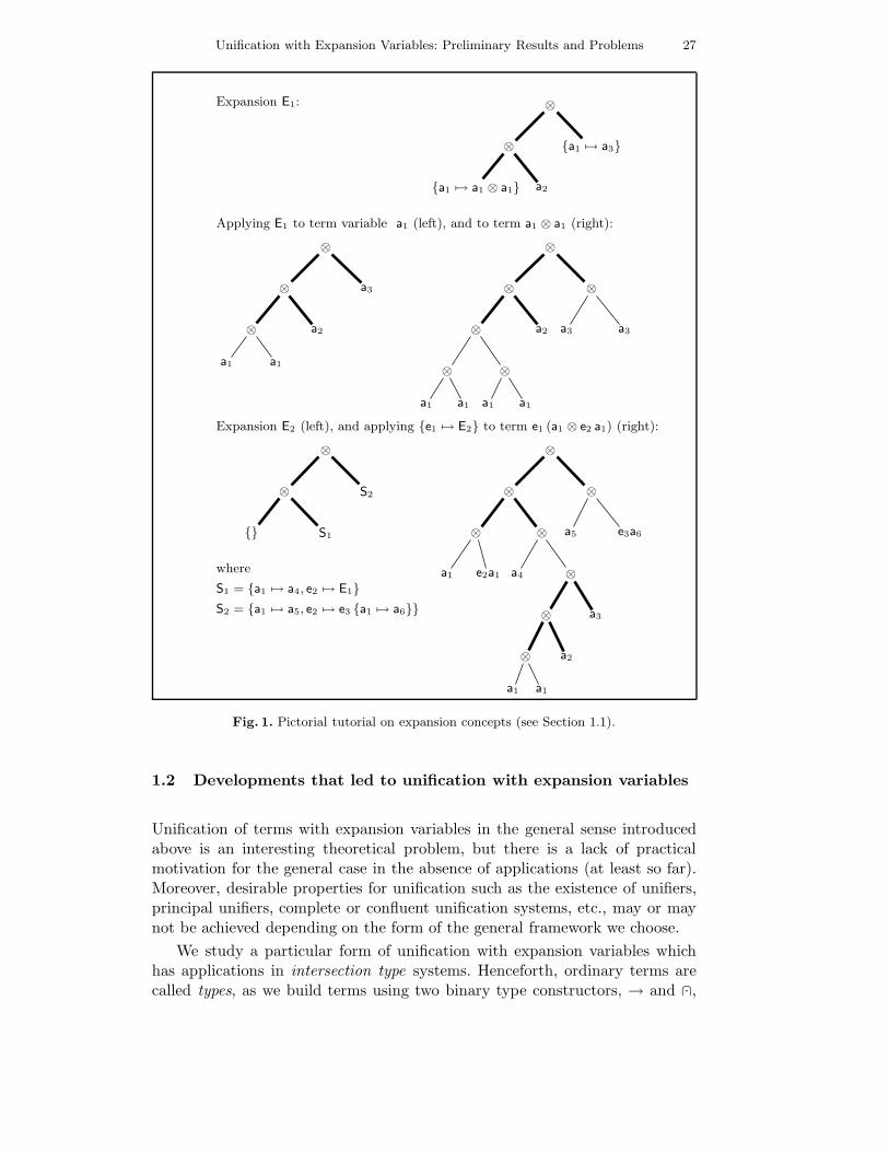
Unification with Expansion Variables: Preliminary Results and Problems 27
Expansion E1: ⊗
⊗ a1 7→ a3
a1 7→ a1 ⊗ a1 a2
Applying E1 to term variable a1 (left), and to term a1 ⊗ a1 (right):
⊗
⊗ a3
⊗ a2
a1 a1
⊗
⊗ ⊗
⊗ a2
⊗ ⊗
a1 a1 a1 a1
a3 a3
Expansion E2 (left), and applying e1 7→ E2 to term e1 (a1 ⊗ e2 a1) (right):
⊗
⊗ S2
S1
⊗
⊗ ⊗
⊗⊗
a4e2a1a1 ⊗
⊗ a3
⊗ a2
a1 a1
a5 e3a6
where
S1 = a1 7→ a4, e2 7→ E1
S2 = a1 7→ a5, e2 7→ e3 a1 7→ a6
Fig. 1. Pictorial tutorial on expansion concepts (see Section 1.1).
1.2 Developments that led to unification with expansion variables
Unification of terms with expansion variables in the general sense introducedabove is an interesting theoretical problem, but there is a lack of practicalmotivation for the general case in the absence of applications (at least so far).Moreover, desirable properties for unification such as the existence of unifiers,principal unifiers, complete or confluent unification systems, etc., may or maynot be achieved depending on the form of the general framework we choose.
We study a particular form of unification with expansion variables whichhas applications in intersection type systems. Henceforth, ordinary terms arecalled types, as we build terms using two binary type constructors, → and .∩,

28 A. Bakewell, A. J. Kfoury
instead of one ⊗, and a special constant ω. Expansions include .∩ and a specialconstant Ω, but not →.2
Beta-unification. The ω-free restriction of the problem we called β-unificationin [9, 13] and other more recent reports. The name β-unification refers to a pre-cise connection. There is a constraint set, i.e., an instance of unification withexpansion variables, for every term of the lambda-calculus. A term is β-stronglynormalizing iff the corresponding constraint set has a unifier. This relationshipwas expounded in [9], where a somewhat different form of expansion variableswas introduced. A theoretical presentation of another important connectionwas described: Constraint-set solving reveals an intersection typing for the cor-responding lambda-calculus term. System I, a system of intersection types withexpansion variables for the lambda-calculus [13], gave a procedure for solving anearly formulation of unification with expansion variables and applied it to inferprincipal typings (not just principal types). Principal typings are important forcompositional program analysis.
Expansions and expansion variables are now being applied and developed inthe framework of System E, a more recent system of intersection types with ex-pansion variables [5]. This has a more sophisticated and intelligible formulationof expansions and expansion variables than System I.
Differences in formulation. There are many notational variants betweenthe present formulation of unification with E-variables and the various earlierformulations based on System I in [9, 11, 10, 13], which are not important. Thecore algebraic setup is similar: Types and constraint were built in the sameway (but without ω). The main difference is in expansions and their semantics.Substitution was not a case of expansion: The leaves of expansions were alwaysholes, denoted . Applying a substitution S to an applied E-variable e, i.e.,[S] (e τ), gave the term-part of S(e) (as in the present formulation), but withthe ith leaf of S(e) replaced by S(〈τ〉i) where 〈τ〉i creates a copy of τ with allthe variables renamed according to a certain scheme. For example,
[e1 7→ .∩] (e1 a1) = a1·1.∩ a1·2
where a1·1 and a1·2 are renamings of a1. To apply substitutions that affect deepnamespaces it was necessary to pre-empt the renamings. Thus the followingsubstitution achieved the same result as e1 7→ .∩ in the present formu-lation:
[e1 7→ , a1·1 7→ a1, a1·2 7→ a1] (e1 a1) = a1.∩ a1
To support this approach there were restrictions on variable names. This makestranslating constraints and their solutions between the present and earlier for-mulations of unification with expansion variables slightly complicated.
2 The purpose of the special constants ω and Ω is explained in Section 2. In papers ontyped lambda-calculi, the binary constructors ∧ and ∩ are often used instead of our .∩.We prefer .∩ to avoid symbol overloading. We use ∩ and ∧ to denote set intersection andlogical conjunction, respectively. Contrary to standard uses of ∩ and ∧, our .∩ is not alwaysassociative, commutative or idempotent.
Unification with Expansion Variables: Preliminary Results and Problems 29
The main result established for the formulation used in System I centresaround the connection between β-unification, β-strong normalisation and ty-pability in the system of intersection types. The restrictions on constraintsindicated above, and other restrictions on substitutions designed to make it fitwell with certain type systems,3 make it difficult to transfer this result to thepresent formulation via a translation because there are admissible solutions inthe present formulation that have no counterpart in System I. However, we areable to establish the same connections and results independently, see Section 4and [3]. In short, what is presented here completely supersedes the formulationused in System I.
1.3 What This Paper Is Not
Apart from the historical connection just reviewed, this paper is not about typesystems and the lambda-calculus. Nor is it about the duplication operationknown as “expansion” in the earlier work on intersection-type systems [17, 15,16]. Nor is it about “expansion variables” as defined and used in our own [9] oreven in [10, 13]. A cursory reading of the forementioned papers makes clear thedifferences with the framework of this paper: The mechanisms we define andbring into play here, in order to formulate problems and resolve them, are notfound in the forementioned papers.
But they are found in the more recent papers on System E [5, 6, 2], wherethey are also mixed with a wide range of issues related to type systems and thelambda-calculus. Our first goal here is to disconnect the concepts of expansionand expansion variable underlying the process of constraint solving from allother issues in System E. This separate examination facilitates the explanationof the key concepts, which are quite natural, and offer new ways of tackling thestill unresolved problems.
1.4 Our Contribution and Organization of This Paper
Once we extract the unification problem from the rest of the System E frame-work (in Section 2), involving a separate formalization in its own right, wepresent:
1. Several modifications of both theoretical and practical interest (in Sec-tion 3).
2. Research directions (in Section 4) and decidability and undecidability re-sults. As with other unification problems, the aim is to design efficient sys-tems that produce most-general unifiers.
3. An outline of preliminary results and a pared-down version of the method-ology we use to obtain them (in Section 5).
3 Specifically, substitutions were restricted to map T-variables to the restricted types (seeDefinition 1).

30 A. Bakewell, A. J. Kfoury
2 Problem Formulation
We first define the syntactic elements that comprise an instance of unificationwith expansion variables in Section 2.1, then the semantics of expansions inSection 2.2, and finally constraints and their unifiers in Section 2.3.
2.1 Syntax
Definition 1 (Types). There are two kinds of variables, expansion variables(E-variables) and type variables (T-variables),
E-Var = ei i ∈ I and T-Var = ai i ∈ J
where I and J are countable subsets of the natural numbers. Metavariables e, aand v range over E-Var, T-Var and Var = E-Var∪T-Var, respectively.4 Restrictedtypes and types are defined as the least sets satisfying:
Typ→ ⊇ T-Var ∪ τ1→ τ2 τi ∈ Typ
Typ ⊇ Typ→ ∪ ω ∪ τ1 .∩ τ2 τi ∈ Typ ∪ e τ e ∈ E-Var and τ ∈ Typ
Metavariable τ and τ range over Typ→ and Typ, respectively. Expressions inTyp→ have constructors of the simply-typed lambda-calculus outermost. Expres-sions in Typ add the binary constructor .∩, E-variables and the constant (ornullary constructor) ω.5
The types are ambiguous, e.g., a .∩ a→ a can be understood as two differenttypes. To disambiguate we assume → and .∩ associate to the right and .∩ bindsmore tightly than →.
Definition 2 (Substitutions and Expansions). If A and B are arbitrarysets, we write f : A _ B to denote a total function f from A to B.6 Substitu-tions and expansions are defined simultaneously as the least sets such that:
Substitution ⊇ ∪ S : Var _ (Typ ∪ Exp) S(a) ∈ Typ and S(e) ∈ Exp
Exp ⊇ Ω ∪ Substitution ∪ eE E ∈ Exp ∪ E1.∩ E2 Ei ∈ Exp
4 We are careful to distinguish between literals and metavariables ranging over literals, andbetween names of particular objects and metavariables ranging over names. Literals andnames are in sans-serif or upright Greek fonts, e.g., e, a, E and τ. Metavariables are in italicor regular Greek fonts, e.g., e, a, E and τ .
5 In System E, the system of intersection types with expansion variables [5] which we dis-cussed in Section 1.2, ω is an important feature and represents the empty intersection.Among other things, it supports analysis of dead-code in terms (more generally, in func-tional programs) and allows for a uniform account of terms containing dummy λ-bindings,e.g., a term of the form ((λx.M)N) where there are no free occurrences of variable x in M .
6 We use the symbol “_” to distinguish it from “→” which is a type constructor.

Unification with Expansion Variables: Preliminary Results and Problems 31
The symbol “” denotes a particular total function from Var to Typ ∪ Exp,recursively defined by:7
= a 7→ a | a ∈ T-Var ∪ e 7→ e | e ∈ E-Var
By Proposition 1 below, is the identity substitution, denoted in Section 1.1;we prefer the less ambiguous . The symbol “Ω” denotes a particular expansion,whose interpretation is formally given by Definition 4 below. We call Ω anannihilator because it maps every type τ to ω and every expansion E to Ω.
Substitutions are sort-preserving total functions from Var to Typ ∪ Exp,whereas expansions are formal expressions built from the binary constructor .∩,unary E-variables, and substitutions or Ω at the leaves.8
Definition 3 (Substitution Support). A substitution S is always a totalfunction on Var whose support is:
support(S) = a ∈ T-Var S(a) 6= a ∪ e ∈ E-Var S(e) 6= e
which may or may not be finite. For convenience and whenever possible, wedefine a substitution by enumerating the restriction to its support, as in Sec-tion 1.1. So a1 7→ a2 is not partial; it is equal to on all variables apart froma1.
2.2 Expansion Semantics
Expansions can be applied to any type or expansion. The definition of applica-tion is the same for the common constructors of both of these sorts.
Definition 4 (Expansion Application). The application of an expansionE to a type τ (respectively, an expansion E1), written [E] τ (resp., [E]E1),returns a type (resp., an expansion). The inductive definition follows, startingwith substitutions which are a special case of expansions:
Applying substitutions to types: Applying substitutions to expansions:
[S]α = S(α) [S]S1 = v 7→ [S] (S1(v)) v ∈ Var
[S] (τ1→ τ2) = [S] τ1→ [S] τ2
[S]ω = ω [S] Ω = Ω
[S] (e τ) = [S(e)] τ [S] (eE) = [S(e)]E
[S] (τ1 .∩ τ2) = [S] τ1 .∩ [S] τ2 [S] (E1.∩ E2) = [S]E1
.∩ [S]E2
7 To understand informally, take the infinite unwinding of its definition. To simplify this,let T-Var and E-Var be the finite sets a1 and e1, for which we get:
= a1 7→ a1, e1 7→ e1a1 7→ a1, e1 7→ e1a1 7→ a1, e1 7→ e1a1 7→ a1, e1 7→ · · ·
This also shows that substitutions are higher-order functions; their result for an E-variableargument can include substitutions.
8 As substitutions are not formal expressions, strictly speaking, every S ∈ Substitution shouldhave a formal symbol, say S#, whose interpretation is the function S. Expansions shouldbe built from S# | S ∈ Substitution instead of Substitution. But this level of precision isnot needed. An alternative is to define substitutions as formal expressions. This approachis used in [5]; it corresponds more directly to the implementation of expansions, but ourconcern here is to reduce the definitional overhead.

32 A. Bakewell, A. J. Kfoury
Applying expansions to types: Applying expansions to expansions:
[Ω] τ = ω [Ω]E = Ω
[eE] τ = e ([E] τ) [eE1]E = e ([E1]E)
[E1.∩ E2] τ = [E1] τ .∩ [E2] τ [E1
.∩ E2]E = [E1]E .∩ [E2]E
Note how the formal definition matches the description in Section 1.1: A sub-stitution distributes down to the outermost variables of its argument then getsapplied, in the usual fashion, whereas an expansion distributes its argumentdown into its leaves and then applies substitutions to it.
Proposition 1 ( Lifts to the Identity). For all types τ and expansions E,it holds that [] τ = τ and []E = E = [E] .
Example 1 (Expansion application). [e1 7→ Ω .∩ .∩ e4 ] e1 (ω→ e2 (a1→ a1))= ω .∩ (ω→ e2 (a1→ a1)) .∩ e4 (ω→ e2 (a1→ a1))
Proposition 2 (Expansion Composition Is Associative). For every typeor expansion X, it holds that [[E1]E2]X = [E1] ([E2]X).
Notation 1 For expansions E1 and E2, let (E1;E2) be shorthand for the com-position [E2]E1, i.e., E1 is applied first and E2 second (opposite to their orderin [E2]E1). By Proposition 2, “;” is associative, so E1;E2;E3 is unambiguous.
2.3 Solutions and Unifiers
In unification theory, a problem instance is a set of constraints, and a unifieris a solution. We adapt these standard concepts to our framework. But first,some notation and definitions on equality and subtyping.
Definition 5 (Equality). Equality of types is determined by an equationaltheory, denoted =Eq, induced by a set Eq of equations.9 Two types τ1 and τ2are equal iff (τ1, τ2) ∈ =Eq, more conveniently written τ1=Eqτ2 or, if the con-text makes clear what Eq is, τ1 = τ2. Technically, =Eq is the least congruencerelation on the set Typ containing Eq. If Eq = ∅, then =Eq is syntactic equal-ity. However, in the presence of ω, we require that Eq contains the followingequations at a minimum:
(1) ω .∩ τ = τ = τ .∩ω for all types τ .
(2) eω = ω for all E-variables e.
Equations (1) make ω a neutral element (or a unit) of the binary .∩, correspond-ing to the intuition that ω is the empty intersection. See footnote 5. Equations(2) are needed for a smooth theory with (1) and are part of the formal setupin [2, 5].
Equations other than (1) and (2) are added to Eq when we consider newtype constructors (such as !) or when we want type constructors to obey newalgebraic laws (such as associativity and commutativity of .∩). See Section 3.
9 We follow standard terminology of universal algebra. See [1], for example.
Unification with Expansion Variables: Preliminary Results and Problems 33
Definition 6 (Subtyping). To determine whether a type is a subtype of an-other, we use a subtyping theory ≤Sub, induced by a set Sub of subtyping pairs.Instead of writing (τ1, τ2) ∈ ≤Sub, we write τ1 ≤Sub τ2 or, if the context makesclear what Sub is, τ1 ≤ τ2. The relation ≤Sub is the least closed under the rules:
τ1=Eqτ2τ1 ≤ τ2
(Eq-≤)(τ1, τ2) ∈ Sub
τ1 ≤ τ2(Sub-≤)
τ1 ≤ τ2 τ2 ≤ τ3τ1 ≤ τ3
(Trans-≤)
τ3 ≤ τ1 τ2 ≤ τ4τ1→ τ2 ≤ τ3→ τ4
(→-≤)τ1 ≤ τ3 τ2 ≤ τ4τ1 .∩ τ2 ≤ τ3 .∩ τ4
( .∩-≤)τ1 ≤ τ2e τ1 ≤ e τ2
(e-≤)
Note that =Eq ⊆ ≤Sub. If Sub = ∅, it is easy to see that τ1=Eqτ2 iff τ1≤Subτ2.What subtyping relations we place in Sub depends on intended applications
and restrictions imposed on type constructors. Some of these are mentioned inSection 3 and again in Section 4 where we discuss research directions. Unlessotherwise stated, we assume Sub = ∅.
Definition 7 (Constraints and Constraint Sets). A constraint is an or-dered pair of types τ1 and τ2, written τ1 ⋖τ2. In the special case when Sub = ∅,we may write the constraint τ1 ⋖τ2 as τ1
.= τ2 instead. If we want to distinguish
the general case from the special case, the first is a subtyping constraint and thesecond an equality constraint. An instance of unification with expansion vari-ables is a finite set of constraints. Metavariables δ and ∆, possibly decorated,range over constraints and constraint sets, respectively.
Example 2 (Constraint Set). Introducing a running example:∆1 = e1 (ω→ e2 (a1→ a1))
.= ω .∩ (e3 a1→ e3 a1) .∩ e4 a1
Definition 8 (Solved Constraint Sets). The predicate solved is defined onconstraints and extended to sets as follows.
solved(τ1 ⋖ τ2) iff τ1 ≤ τ2;solved(∆) iff solved(δ) for every δ ∈ ∆.
A solved constraint remains solved after the application of any expansion.
Definition 9 (Solutions and Unifiers). If δ is the constraint τ1 ⋖ τ2 andE an expansion, then [E] δ denotes the constraint [E] τ1 ⋖ [E] τ2. If ∆ is aconstraint set, then [E] ∆ denotes the constraint set [E] δ δ ∈ ∆ . ExpansionE is a solution of constraint set ∆ iff solved([E] ∆).
In the special case when Sub = ∅ and constraints are equality constraints,we may call a solution E a unifier, to emphasize that it equalizes the two sidesof each constraint.
Remark 1. The annihilator Ω trivially solves all constraints, which we thus callthe trivial solution. In general, Ω is not the solution we want, if only because itcannot be a principal solution when other non-trivial solutions exist. We thinkof Ω as a solution of “last resort”, when everything else has failed.10
10 This is the way we deal with Ω in [3]. What plays the role of Ω here is the expansion ω
in [3]. It is perhaps unfortunate that, in [3] following [5], we used the same symbol ω todenote a type (as we do here) and an expansion (as we do not do here).

34 A. Bakewell, A. J. Kfoury
3 Other Versions of Unification with Expansion Variables
There is much to investigate in relation to the the fundamental frameworkpresented in Section 2. There are more details in the report [3], which is only abeginning, as it uncovers more problems than it solves. We consider restrictionsof the fundamental framework to make more tractable some of the theoreticalproblems, and consider generalizations for possible applications.
Omega-Free Unification. This simple restriction consists in omitting ω fromthe syntax of types (Definition 1) and Ω from the syntax of expansions (Defi-nition 2), as well as omitting every part dealing with ω and Ω in each of Defi-nition 4 and Definition 5. In particular, this makes Eq = ∅, so that =Eq is justsyntactic equality. By translating the mechanism of substitution compositionused in [13] to expansion composition as defined here, consistently throughout,we essentially obtain ω-free unification with expansion variables, for which wehave the most complete set of results so far.
Ranked Unification. The rank of a type τ is the smallest integer k such thatthe path between the root of τ and any occurrence of “ .∩” in τ goes to the left ofan occurrence of “→” less than k times. Formally, we stratify types as follows.The sets Typ0 and Typk, for every k > 1, are the least such that:
Typ0 ⊇ T-Var ∪ τ1→ τ2 τi ∈ Typ0 ∪ ω ∪ e τ e ∈ E-Var and τ ∈ Typ0
Typk ⊇ Typk−1 ∪ τ1→ τ2 τ1 ∈ Typk−1 and τ2 ∈ Typk
∪ τ1 .∩ τ2 τi ∈ Typk ∪ e τ e ∈ E-Var and τ ∈ Typk
Clearly Typ =⋃
k>0 Typk. Define rank(τ) as the least k > 0 such that τ ∈ Typk.Let E be an expansion and δ the constraint τ1 ⋖ τ2. If E is a unifier of δ, wesay E is a rank-k unifier of δ if maxrank([E] τ1), rank([E] τ2) 6 k. We say Eis rank-k unifier of the constraint set ∆ if E is a rank-k unifier of every δ ∈ ∆.
AC and ACI Unification. Generalizations required by potential applicationswill make the binary constructor .∩ satisfy one or more of:
(A) associativity τ1 .∩ (τ2 .∩ τ3) = (τ1 .∩ τ2) .∩ τ3 for all types τ1, τ2 and τ3.(C) commutativity τ1 .∩ τ2 = τ2 .∩ τ1 for all types τ1 and τ2.(I) idempotence τ .∩ τ = τ for all types τ .
With AC, and a fortiori ACI, we need to impose an additional requirement forthe theory to work smoothly (see [5]). This is expressed by an equation relatingE-variables to .∩, allowing the first to distribute over the second, as follows:
(D) e (τ1 .∩ τ2) = e τ1 .∩ e τ2 for all E-variables e and types τ1 and τ2.
Equations (A), (C), (I) and (D) are added to Eq and the equational theory=Eq modified accordingly.
Unification+Bang. In general, intersection types provide more precise typ-ings when they are linear, i.e., when the binary constructor .∩ is not idempotent.However, linear types have a high cost, typically making unification computa-tionally unfeasible. We can relax linearity in a controlled way by introducing
Unification with Expansion Variables: Preliminary Results and Problems 35
the unary type constructor “!”, and adding the following subtyping relation toSub:11
! τ ≤ τ .∩ τ for all types τ .
In the presence of !, we also add the following equations to Eq, dictated bysemantic considerations:
(1) ! ω = ω (! is absorbed by ω).(2) ! ! τ = ! τ (! is idempotent) for all types τ .(3) e ! τ = ! e τ (E-variables and ! commute) for all E-variables e and types τ .(4) ! (τ1 .∩ τ2) = ! τ1 .∩ ! τ2 (! distributes over .∩) for all types τ1 and τ2.
Introducing !, subject to the subtyping and equations above, makes it possible toobtain the precision of linear types when it is useful, while preventing linearityfrom getting in the way when it is not needed. More on the use of ! can be foundin [5, 6] in relation to building a flexible type system for the lambda calculus.
The integration of ! with E-variables is straightforward. In addition to a casefor ! in the definitions of Typ and Exp (in Definition 1 and Definition 2), we addthe following rules to expansion and substitution application (see Definition 4):
[!E]X = ! [E]X and [S] !X = ! [S]X
where X is a type or an expansion. But this also complicates the algebra oftypes considerably and their unification accordingly.
Other Versions of Unification. Restrictions and generalizations can be com-bined, guided by theoretical or practical considerations. For example, ω-freeranked unification imposes the restrictions of both the ω-free and ranked cases.
4 Research Directions
There are standard questions in unification theory that immediately transfer toour setting. Given an arbitrary unification instance ∆, we ask:
1. Decidability : Is it decidable whether ∆ has a unifier?(a) If yes, what is the complexity of the decision procedure?(b) If yes and ∆ has a unifier, what is the complexity of building a unifier?(c) If no, what meaningful restrictions on ∆ make the problem decidable?
2. Principality : If ∆ has a unifier, does it have a principal unifier from which allother unifiers can be obtained (by some formal mechanism, such as functioncomposition, in our case expansion composition)?
These questions are typically further refined. For example, in relation to com-plexity we may ask for upper bounds (usually easier), and lower bounds (usu-ally harder). Note that questions 1.(a) and 1.(b) are not equivalent.12 Naturally,
11 For an intuition, think of ! τ as “an object of type ! τ can be used at type τ any number oftimes”, and τ .∩ τ as “an object of type τ .∩ τ can be used at type τ only twice”.
12 A case in point is first-order unification. It is decidable whether an instance of first-order uni-fication has a unifier in low-degree polynomial time. However, when there is a unifier, build-ing a most general unifier is low-degree polynomial time only with clever data-structuresthat represent terms by dag’s instead of trees.

36 A. Bakewell, A. J. Kfoury
such questions arise for unification with expansion variables, or any of the re-strictions/generalizations mentioned in Section 3 and Section 1.1. Currently,we have the most complete set of answers (and proof techniques) for ω-freeunification, for which the most significant result is the following.
Theorem 2 (ω-Free Unification With E-Variables Is Undecidable).
1. There is an algorithm A which, given an arbitrary term M of the purelambda calculus, returns an ω-fee instance A(M) of unification with ex-pansion variables such that: M is β-strongly normalising iff A(M) has aunifier.
2. It is undecidable whether an arbitrary ω-free instance has a unifier.
Only the proof of part 1 in the theorem is complicated. Part 2 is an immediateconsequence of part 1, using the undecidability of β-strong normalization ofterms of the lambda calculus [4]. This undecidability result does not imply theundecidability of any of the other unification cases mentioned in Section 3.Inparticular, as noted in Remark 1, any modification of the framework that in-cludes a type constant such as ω and a corresponding expansion such as Ω istrivially decidable. This corresponds to the fact that all terms can be assignedthe type ω in intersection type systems that include ω such as System E. Decid-able modifications also arise when there are no expansion constructors exceptE-variables, or only one constructor.
5 Proposed Methodology
Rewriting techniques provide powerful tools for analyzing and solving problemsin other forms of unification. We use a methodology inspired by such techniques.We have already developed elements of this approach, although not to the pointof enabling us to tackle all of the problems we raised in Section 4.
In this section we present a streamlined and highly condensed illustration ofthe proposed methodology: This is a very simple rewrite system that generatesunifiers for constraint sets built in the most basic version of the framework ofSection 2, with Sub = ∅ (Definition 6). As Sub = ∅, we write constraints asequality constraints, i.e., we write τ1
.= τ2 instead of τ1 ⋖ τ2.
The unification procedure interleaves two phases, simplification and rewrit-ing. The same approach is used in the more powerful procedures consideredin [3]. But first, some helpful notation.
Notation 3 1. Let e be a metavariable ranging over finite sequences of E-variables, including the empty sequence ε.
2. A constraint of the form e τ1.= e τ2, where τ1 and τ2 do not have applica-
tions of the same E-variable outermost, may be written e (τ1.= τ2). Call e
the prefix of such a constraint.3. Let the notation e/S be shorthand for the substitution e 7→ eS. Think of
such a substitution as acting under e, or in namespace e.4. We extend the “/” notation to sequences of E-variables: e · e/S means e/(e/S)
and ε/S means S.
Unification with Expansion Variables: Preliminary Results and Problems 37
Definition 10 (Simplification). The function simplify factors out commonstructure and eliminates solved constraints:
simplify(∅) = (∅),
simplify(δ ∪∆) = simplify(δ) ∪ simplify(∆),
simplify(δ) =
simplify(e τ1.= e τ2, e τ ′1
.= e τ ′2) if δ is e (τ1 .∩ τ
′1.= τ2 .∩ τ
′2),
simplify(e τ1.= e τ2, e τ ′1
.= e τ ′2) if δ is e (τ1→ τ ′1
.= τ2→ τ ′2),
∅ if δ is τ.= τ ,
δ otherwise.
For an arbitrary constraint set ∆, solved(∆) is true iff simplify(∆) = ∅. Simpli-fication is sound in the sense that, for all constraint sets ∆ and all expansionE, it holds solved([E]∆) iff solved([E] (simplify(∆))).
Example 3. simplify(ω .∩ (ω→e2 a1) .∩ e4 (ω→e2 a1).=ω .∩ (e3 a1→e3 a1) .∩ e4 a1)
= ω.= e3 a1, e2 a1
.= e3 a1, e4 ((ω→ e2 a1)
.= a1)
Definition 13 introduces the relation =S=⇒, a one-step rewrite rule, which partly
solves a constraint with substitution S. A few preliminary concepts are needed.
Definition 11 (Topmost Expansion Extraction). By induction on types:
extract(τ ) =
extract(ω) = Ω
extract(e τ) = e (extract(τ))extract(τ1 .∩ τ2) = extract(τ1) .∩ extract(τ2)
In words, the topmost expansion of τ is the largest tree of expansion constructorsfrom the root of τ down to where non-expansion constructors are encountered,with the identity substitution or annihilator substitution Ω at each leaf.
Example 4 (extraction). extract(ω .∩ (e3 a1→ e3 a1) .∩ e4 a1) = Ω .∩ .∩ e4
The “outer-part unifier” in the next definition creates substitutions for variablesthat occur outermost, i.e., in the top-level namespace. We generate substitutionunifiers: Forming expansion unifiers from a set of substitution unifiers is easilydone separately.
Definition 12 (Outer-Part Unifier). The binary relation −unifier−−−→ relates con-straints and substitutions according to the following rule:
e (τ1.= τ2) −
unifier−−−→
e/a 7→ τ if τ1, τ2 = a, τ (T-unify)
e/e 7→ extract(τ) if τ1, τ2 = e τ , τ (E-unify)
Recall that in constraint e (τ1.= τ2) there is no E-variable e such that τ1 = e τ ′1
and τ2 = e τ ′2, by Notation 3. And τ refers to a restricted type, by Definition 1.
– (T-unify) solves a constraint where one side is a T-variable and the otherside is a restricted type, if a is not in the empty namespace of τ .
38 A. Bakewell, A. J. Kfoury
– (E-unify) solves the topmost part of a constraint by substituting the topmostexpansion of one side for the E-variable e on the other side, provided theargument of e is a restricted type.
Remark 2. The (T-unify) and (E-unify) rules do not include occur checks onthe variables in the empty namespaces of τ and extract(τ) respectively. Addingthese conditions prevents perpetual rewriting of constraint sets such ase1 a1
.= e1 a2
.∩ e1 a2.
Example 5 (Outer-Part Unifier). e2 (a1→ a1).= e3 a1 −
unifier−−−→ e3 7→ e2
Definition 13 (One-Step and Multi-Step Rewriting). The one-step re-
write rule =S=⇒ does two things: It first (non-deterministically) outer-part unifies
one of the constraints, applying the resulting substitution S to the entire con-straint set, and then it simplifies:
∆ =S=⇒ simplify([S]∆) if there is δ ∈ simplify(∆) such that δ −unifier−−−→ S.
We define ∆ ==⇒ ∆′ if there is a substitution S such that ∆ =S=⇒ ∆′. The multi-
step rewrite rule ==⇒⇒ is the reflexive transitive closure of ==⇒. Formally, we firstdefine for all ∆,∆1 and ∆2:
∆ =
=⇒⇒ simplify(∆) and
∆ =S1;S2===⇒⇒ ∆2 if ∆ =
S1=⇒ ∆1 and ∆1 =
S2=⇒⇒ ∆2.
We then define ∆ ==⇒⇒ ∆′ if there is a substitution S such that ∆ =S=⇒⇒ ∆′.
Example 6 (Rewriting).
∆1 =e1 7→Ω .∩ .∩ (e4 )===========⇒ ω
.= e3 a1, e2 (a1→ a1)
.= e3 a1, e4 (ω→ e2 (a1→ a1)
.= a1)
=e4/a1 7→ω→e2 (a1→a1)=============⇒ ω
.= e3 a1, e2 (a1→ a1)
.= e3 a1
=e3 7→e2 ======⇒ ω
.= e2 a1, e2 (a1→ a1
.= a1)
=e2 7→Ω====⇒ ∅
Theorem 4 (Soundness of Rewriting). If ∆ =S=⇒⇒ ∅ then solved([S] ∆), i.e.,
S is a unifier of ∆.
Thus a rewrite sequence resulting in ∅ produces a unifier. The length of arewrite sequence is the number of applications of the one-step rewrite rule whichit comprises. Infinite rewrite sequences have an unbounded length; terminatingrewrite sequences have a finite length.
Remark 3 (Incompleteness). There are constraints, such as ω.= a1→ a1, with
expansion-unifiers, that ==⇒ cannot solve. There are also constraints with substi-tution-unifiers that ==⇒ cannot solve; for an idea of the issues involved, witness:
∆2 = e1 (ω.= a1→ a1), e1 a1
.= a1
.∩ a1 =e1 7→ .∩======⇒ ∆2 = ω
.= a1→ a1
Unification with Expansion Variables: Preliminary Results and Problems 39
∆2 is soluble with S3 = e1 7→ Ω .∩Ω, a1 7→ ω but the simple system has vari-ous inadequacies, preventing the discovery of such unifiers: It always assigns out-ermost E-variables the topmost extraction, rather than allowing lesser extrac-tions; it does not rename variables under an expanded E-variable; and, most rel-evant for ∆2, it does not introduce fresh E-variables so that such solutions can bebuilt up gradually, e.g. [S3]∆2 = [e1 7→ e2
.∩ e2; e2 7→ Ω; a1 7→ ω]∆2.
Remark 4 (Termination and Non-Termination). Some constraints have infiniterewrite sequences. For example, the following rewrite produces a kind of repeat-able cycle:
∆3 = e1 ((e2 ((e3 a1→a2) .∩ e3 a1))→e4 a2).= e2 ((e3 a1→a2) .∩ e3 a1), e4 a2
.= a2
=e4 7→;e1 7→e2 ( .∩e3 );e2 e3/a1 7→(e2 ((e3 a1→a2) .∩e3 a1))→e4 a2======================================⇒⇒ [e2]∆3
So termination depends on the rewrite strategy because ∆3 is solved by anotherstrategy that generates the substitutions e2 7→ e1 ; e1 7→ Ω; e4 7→ . In-finite rewriting is an essential ingredient for the correspondence to β-reduction(mentioned in Section 1.2).
Theorem 5 (Completeness of Rewriting for a Special Case). The sim-ple rewrite system presented in this section is complete for the special case wheninstances ∆ satisfy the conditions spelled out in [3, 2].13 That is, for such a ∆,
if ∆ has a unifier then ∆ =S=⇒⇒ ∅ for some substitution S.
References
1. F. Baader and T. Nipkow. Term Rewriting and All That. Cambridge University Press,1998.
2. A. Bakewell, S. Carlier, A. J. Kfoury, and J. B. Wells. Exact intersection typing inferenceand call-by-name evaluation. Technical report, Department of Computer Science, BostonUniversity, Dec. 2004.
3. A. Bakewell and A. J. Kfoury. Unification with expansion variables. Technical report,Department of Computer Science, Boston University, Dec. 2004.
4. H. P. Barendregt. The Lambda Calculus: Its Syntax and Semantics. North-Holland,revised edition, 1984.
5. S. Carlier, J. Polakow, J. B. Wells, and A. J. Kfoury. System E: Expansion variables forflexible typing with linear and non-linear types and intersection types. In ProgrammingLanguages & Systems, 13th European Symp. Programming, vol. 2986 of LNCS, pp. 294–309. Springer-Verlag, 2004.
6. S. Carlier and J. B. Wells. Type inference with expansion variables and intersection typesin System E and an exact correspondence with β-reduction. In Proc. 6th Int’l Conf.Principles & Practice Declarative Programming, 2004.
7. D. D. Champeaux. About the paterson-wegman linear unification algorithm. J. Comput.Syst. Sci., 32(1):79–90, 1986.
8. A. J. Kfoury. Beta-reduction as unification. A refereed extensively edited version is [9].This preliminary version was presented at the Helena Rasiowa Memorial Conference, July1996.
13 These conditions cannot be presented within the confines of this extended abstract. Butsuffice it to say that if the constraint set ∆ corresponds to the typability of a term of thelambda calculus in a certain system of intersection types, then ∆ satisfies the conditions.

40 A. Bakewell, A. J. Kfoury
9. A. J. Kfoury. Beta-reduction as unification. In D. Niwinski, ed., Logic, Algebra, andComputer Science (H. Rasiowa Memorial Conference, December 1996), Banach CenterPublication, Volume 46, pp. 137–158. Springer-Verlag, 1999. Supersedes [8] but omits afew proofs included in the latter.
10. A. J. Kfoury, G. Washburn, and J. B. Wells. Implementing compositional analysis usingintersection types with expansion variables. In Proceedings of the 2nd Workshop on In-tersection Types and Related Systems, 2002. The ITRS ’02 proceedings appears as vol.70, issue 1 of Elec. Notes in Theoret. Comp. Sci.
11. A. J. Kfoury and J. B. Wells. Principality and decidable type inference for finite-rankintersection types. In Conf. Rec. POPL ’99: 26th ACM Symp. Princ. of Prog. Langs., pp.161–174, 1999. Superseded by [13].
12. A. J. Kfoury and J. B. Wells. Principality and type inference for intersection types usingexpansion variables. Supersedes [11], Aug. 2003.
13. A. J. Kfoury and J. B. Wells. Principality and type inference for intersection types usingexpansion variables. Theoret. Comput. Sci., 311(1–3):1–70, 2004. Supersedes [11]. Foromitted proofs, see the longer report [12].
14. M. Paterson and M. Wegman. Linear unification. J. Comput. Syst. Sci., 16(2):158–167,1978.
15. S. Ronchi Della Rocca. Principal type schemes and unification for intersection type dis-cipline. Theoret. Comput. Sci., 59(1–2):181–209, Mar. 1988.
16. S. Ronchi Della Rocca and B. Venneri. Principal type schemes for an extended typetheory. Theoret. Comput. Sci., 28(1–2):151–169, Jan. 1984.
17. S. J. van Bakel. Intersection Type Disciplines in Lambda Calculus and Applicative TermRewriting Systems. Ph.D. thesis, Catholic University of Nijmegen, 1993.
R-Unification thanks to SynchronizedContext-Free Tree Languages
Pierre Rety, Jacques Chabin, and Jing Chen
LIFO - Universite d’Orleans, B.P. 6759, 45067 Orleans cedex 2, FranceE-mail: rety, chabin, [email protected]
http://www.univ-orleans.fr/SCIENCES/LIFO/Members/rety
Abstract. Expressing descendants or the rewrite relation by tree-(tuple) lan-guages allows to deal with R-matching and R-unification problems. We presentin addition a new class of tree-tuple languages, more expressive than formerones, but having the same properties. Thanks to this new class, we hope tosolve more interesting R-matching and R-unification problems.
1 The General Method
Given a confluent term rewrite system R, computing descendants (i.e. successorsby rewriting) can be applied to R-matching and R-unification. Indeed the R-matching problem t ⊳R t′ has at least one solution θ iff ∃s, tθ →∗
R s ∗R ← t′,
which is equivalent to check that
R∗(tσ | σ ∈ Subst) ∩R∗(t′) 6= ∅
where Subst is the set of all substitutions and R∗(E)def= s | ∃e ∈ E, e→∗
R sare the descendants of the set of terms E. In the same way, and if we assumethat t and t′ do not share variables, the R-unification problem t
.=R t′ has at
least one solution iff
R∗(tσ | σ ∈ Subst) ∩R∗(t′σ′ | σ′ ∈ Subst) 6= ∅
The above remarks can be used to decide R-matchability or R-unifiability,but do not allow to express the possible R-matches or R-unifiers. However if wecan compute the binary relation →∗
R by expressing a set of pairs of terms, wecan in addition express the matched terms, i.e. tθ, tθ =R t′ (or the unifiedterms in a similar way), by computing
M = Π1((tσ, σ ∈ Subst 1⋊⋉1 →∗R) 2⋊⋉1 ( ∗
R← 2⋊⋉1 t′))
where Π1 is the projection onto the first component, and T i⋊⋉j T′ denotes the
natural join (like in a relational database) between the i-th component of T andthe j-th component of T ′ 1. Now, if we can solve the “set syntactic-matchingproblem”, i.e. compute θ ∈ Subst, tθ ∈ M, we get the R-matches. We canget R-unifiers in a similar way.
2 Using Existing Tree-(tuple) Languages
Some tree-(tuple) languages allow to achieve the general method presented inthe previous section.
1 Note that computing →∗R allows to compute the descendants because R∗(E) = Π2(E 1⋊⋉1
→∗R).
41

42 P. Rety, J. Chabin, J. Chen
2.1 By computing descendants
- Using regular tree languages.If t and t′ are linear, then tσ | σ ∈ Subst and t′σ′ | σ′ ∈ Subst areregular languages. Moreover regular tree languages are closed under inter-section, and emptiness is decidable. Therefore for every rewrite system Rthat preserves recognizability2 , R-matchability of problems t ⊳R t′ s.t. t islinear is decidable, and R-unifiability of linear equations is decidable. Strongrestrictions ensuring recognizability preservation have been studied [1, 4, 3,9, 12, 8, 11].
- Using context-free tree languages.Assume that the rewrite system does not preserve recognizability, but sat-isfies the following property : E is regular implies R∗(E) is context-free [10].However context-free languages are not closed under intersection, but areclosed under intersection with a regular language. Therefore, we need toassume in addition that t′ is irreducible in the matching problem t⊳R t
′ sothat R∗(t′) = t′ is regular. In the linear unification problem t
.=R t′,
we need to assume that R is left-linear and constructor-based, and t′ con-tains only constructors and variables, so that E = t′σ′ | σ′ ∈ Subst ∧σ′ is normalized is regular and contains only normalized terms, and conse-quently R∗(E) = E is regular.
2.2 By expressing →∗
R
Here, tree-tuple languages are needed. The class of synchronized tree-tuple lan-guages, first presented thanks to Tree-Tuple Synchronized Grammars (TTSG)[5], then extended thanks to the so-called Constraint Systems (CS) [2], andfinally extended using a logic-programming framework [7] called CS-programs,allows to express →∗
R [6] in a number of cases. Moreover, thanks to the logic-programming formalism, the “set syntactic-matching problem” is trivially solv-able. Therefore we can express the R-matches (or R-unifiers) and (more inter-esting) handle them.
3 Merging Context-free and Synchronized Languages
Context-free tree languages and synchronized tree-tuple languages have thesame properties : they are closed under union, closed under intersection (of onetuple-component) with a regular tree language, membership and emptiness aredecidable.
In order to increase expressivity, we have defined a new class of tree-tuplelanguages : the synchronized context-free languages, obtained by mixing theprevious ones, and we are proving that the properties recalled above still hold.This new class should allow to express both descendants and →∗
R in more casesthan before, thanks to its bigger expressivity.
2 I.e. E is regular implies R∗(E) is regular.
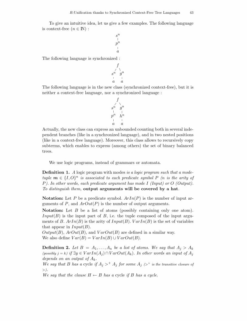
R-Unification thanks to Synchronized Context-Free Tree Languages 43
To give an intuitive idea, let us give a few examples. The following languageis context-free (n ∈ IN) :
sn
pn
a
The following language is synchronized :
f
sn
a
gn
a
The following language is in the new class (synchronized context-free), but it isneither a context-free language, nor a synchronized language :
f
sn
pn
a
gn
hn
a
Actually, the new class can express an unbounded counting both in several inde-pendent branches (like in a synchronized language), and in two nested positions(like in a context-free language). Moreover, this class allows to recursively copysubterms, which enables to express (among others) the set of binary balancedtrees.
We use logic programs, instead of grammars or automata.
Definition 1. A logic program with modes is a logic program such that a mode-tuple m ∈ I,On is associated to each predicate symbol P (n is the arity ofP ). In other words, each predicate argument has mode I (Input) or O (Output).To distinguish them, output arguments will be covered by a hat.
Notation: Let P be a predicate symbol. ArIn(P ) is the number of input ar-guments of P , and ArOut(P ) is the number of output arguments.
Notation: Let B be a list of atoms (possibly containing only one atom).Input(B) is the input part of B, i.e. the tuple composed of the input argu-ments of B. ArIn(B) is the arity of Input(B). V arIn(B) is the set of variablesthat appear in Input(B).Output(B), ArOut(B), and V arOut(B) are defined in a similar way.We also define V ar(B) = V arIn(B) ∪ V arOut(B).
Definition 2. Let B = A1, . . . , An be a list of atoms. We say that Aj > Ak
(possibly j = k) if ∃y ∈ V arIn(Aj)∩V arOut(Ak). In other words an input of Aj
depends on an output of Ak.We say that B has a cycle if Aj >
+ Aj for some Aj (>+ is the transitive closure of
>).We say that the clause H ← B has a cycle if B has a cycle.

44 P. Rety, J. Chabin, J. Chen
Example 1. Q(x, s(y)), R(y, s(x)) (x, y are variables) has a cycle because Q >R > Q.
Definition 3. A Synchronized Context-Free program (S-CF program) Prog isa logic program with modes, whose clauses H ← B both satisfy :
- Input(H).Output(B) ( . is the tuple concatenation) is a linear tuple of variables,i.e. each tuple-component is a variable, and each variable occurs only once.
- B does not have a cycle.
Given a predicate symbol P without input arguments, the tree-(tuple) languagegenerated by P is L(P ) = t ∈ (TΣ)ArOut(P ) | P (t) ∈ Mod(Prog), whereMod(Prog) is the least Herbrand model of Prog. L(P ) is called SynchronizedContext-Free language (S-CF language).
If in addition every clause H ← B of Prog satisfies :
- Output(H).Input(B) ( . is the tuple concatenation) is a linear tuple, i.e. eachvariable of Output(H).Input(B) occurs only once,
then Prog is said non-copying.
Remark 1. - If a predicate symbol P has no input argument, this means thatthe outputs of P do not depend on a given input value (like in a regularlanguage). Therefore, a S-CF program whose predicate symbols do not haveinput arguments, is called synchronized program. It generates a synchronizedtree-(tuple) language. This class of languages has already been studied in[7, 6]. In these papers, synchronized programs are called cs-programs.
- If a predicate symbol P has several output arguments, this means that theseoutput arguments are linked (synchronized) together. Therefore, a S-CFprogram whose predicate symbols have only one output argument, is calledcontext-free program (without synchronization). It generates a context-freetree language.
- A non-copying context-free program whose predicate symbols have no inputarguments, is called regular program. It generates a regular tree language.
Example 2. (x, y are variables)
Prog = P (s(x), y)← P (s(x), y)
is not a S-CF program because Input(H).Output(B) = (y, s(x)) is not a tupleof variables.
Prog′ = P ′(s(x), y)← P ′(x, s(y))
is a S-CF program because Input(H).Output(B) = (y, x) is a linear tuple ofvariables, and there is no cycle. Prog′ is not copying becauseOutput(H).Input(B) =(s(x), s(y)) is a linear tuple.
Example 3. (for n ∈ IN, fn(a) is the term f(f(...f(a))) where f occurs n times)
Prog = S( c
x y
)← P (x, y, a, b). P (f
x
, g
y
, x′, y′)← P (x, y, h
x′
, i
y′
). P (x, y, x, y)←
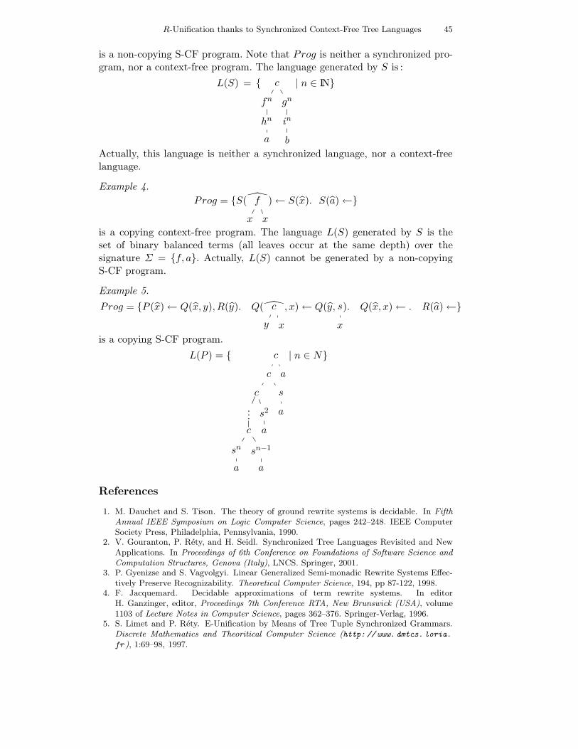
R-Unification thanks to Synchronized Context-Free Tree Languages 45
is a non-copying S-CF program. Note that Prog is neither a synchronized pro-gram, nor a context-free program. The language generated by S is :
L(S) = c
fn
hn
a
gn
in
b
| n ∈ IN
Actually, this language is neither a synchronized language, nor a context-freelanguage.
Example 4.
Prog = S( f
x x
)← S(x). S(a)←
is a copying context-free program. The language L(S) generated by S is theset of binary balanced terms (all leaves occur at the same depth) over thesignature Σ = f, a. Actually, L(S) cannot be generated by a non-copyingS-CF program.
Example 5.
Prog = P (x)← Q(x, y), R(y). Q( c
y x
, x)← Q(y, s
x
). Q(x, x)← . R(a)←
is a copying S-CF program.
L(P ) = c
c
c
...
c
sn
a
sn−1
a
s2
a
s
a
a
| n ∈ N
References
1. M. Dauchet and S. Tison. The theory of ground rewrite systems is decidable. In FifthAnnual IEEE Symposium on Logic Computer Science, pages 242–248. IEEE ComputerSociety Press, Philadelphia, Pennsylvania, 1990.
2. V. Gouranton, P. Rety, and H. Seidl. Synchronized Tree Languages Revisited and NewApplications. In Proceedings of 6th Conference on Foundations of Software Science andComputation Structures, Genova (Italy), LNCS. Springer, 2001.
3. P. Gyenizse and S. Vagvolgyi. Linear Generalized Semi-monadic Rewrite Systems Effec-tively Preserve Recognizability. Theoretical Computer Science, 194, pp 87-122, 1998.
4. F. Jacquemard. Decidable approximations of term rewrite systems. In editorH. Ganzinger, editor, Proceedings 7th Conference RTA, New Brunswick (USA), volume1103 of Lecture Notes in Computer Science, pages 362–376. Springer-Verlag, 1996.
5. S. Limet and P. Rety. E-Unification by Means of Tree Tuple Synchronized Grammars.Discrete Mathematics and Theoritical Computer Science (http: // www. dmtcs. loria.fr ), 1:69–98, 1997.
46 P. Rety, J. Chabin, J. Chen
6. S. Limet and G. Salzer. Proving properties of term rewrite systems via logic programs.In proceedings of RTA 2004, volume 3091 of LNCS, pages 170–184. Springer Verlag, 2004.
7. Sebastien Limet and Gernot Salzer. Manipulating tree tuple languages by transform-ing logic programs. In Ingo Dahn and Laurent Vigneron, editors, Electronic Notes inTheoretical Computer Science, volume 86. Elsevier, 2003.
8. C. Loding. Model-checking Infinite Systems Generated by Ground Tree Rewriting. InProceedings of the 7th Conference on Foundations of Software Science and ComputationStructures. LNCS, Springer, 2002.
9. P. Rety. Regular Sets of Descendants for Constructor-based Rewrite Systems. In Proceed-ings of the 6th international conference LPAR, number 1705 in Lecture Notes in ArtificialIntelligence (LNAI), Tbilisi, Republic of Georgia, 1999. Springer Verlag.
10. P. Rety and J. Vuotto. Context-free tree languages for descendants. In 5th Workshop onRule-Based Programming (RULE’2004). Proceedings in ENTCS vol 124(1), 2005.
11. H. Seki, T. Takai, F. Youhei, and Y. Kaji. Layered Transducing Term Rewriting Sys-tem and its Recognizability Preserving Property. In 13th International Conference RTA,volume 2378 of Lectures Notes in computer Science. Springer-Verlag, 2002.
12. T. Takai, Y. Kaji, and H. Seki. Right-linear finite path overlapping term rewriting systemseffectively preserve recognizability. In L. Bachmair, editor, Proceedings 11th ConferenceRTA, Norwich (UK), volume 1833 of LNCS, pages 246–260. Springer-Verlag, 2000.

Symbolic Debugging in Polynomial Time
Christopher Lynch1 and Barbara Morawska2
1 Department of Computer Science, Box 5815, Clarkson University, Potsdam, NY13699-5815, USA, E-mail: [email protected]
2 Chair for Automata Theory, Institute for Theoretical Computer Science, DresdenUniversity of Technology, Germany, E-mail: [email protected]
Abstract. We show how to use Sorts and Normal Forms to speed up theNarrowing Procedure. Even when an equational theory is closed under Super-position, Narrowing may not terminate. When an equational theory is closedunder Paramodulation Narrowing terminates, but it may have NP complexity.We show that it is possible in some equational theories to use Sorts and NormalForms to model well-formed terms to force Narrowing to terminate with lineartime complexity. We give some real examples which have linear behavior, suchas the theory of lists. We also extend the theory of lists to the theory of listsplus length. We show how these results are useful in debugging.
1 Introduction
When we reason about programs, we must take into account the data struc-tures that are used in the programs. Reasoning about programs then takes placemodulo an equational theory of the data structures used in the programs. Thereare general inference procedures, such as Superposition, which allow such rea-soning for any equational theory. However, these procedures are undecidable ingeneral. Therefore, it is necessary to give a better analysis of the decidabilityand running time of these procedures for specific data structures.
For example, [1] shows how rewriting techniques can be used for verificationof programs modulo the theory of lists and the theory of arrays. They showthat the problem of program verification is the problem of showing if one setof ground equations implies another ground equation, modulo the theory ofthe data structures used in the program. They show that the Superpositioninference system will halt when solving this problem for the theory of lists andthe theory of arrays. In [3] it is shown that the problem can be solved modulothe theory of lists in O(nlg(n)).
The problem of program verification is a universal problem. We want to showthat the precondition implies the postcondition for all values of the variablesused in the program. In this paper, we consider a different problem, which wecall the symbolic debugging problem. Suppose we want to know if is is possibleto follow a certain path in the program. Furthermore, suppose we want toknow for what values of the variables a certain path will be taken. A pathin the program can be represented by a set of equations and disequations,which represent the conditions appearing at each choice point in the program.Therefore, the problem we need to solve is the problem of E-unification of thatset of equations and disequations. If the E-unification problem has a solution,then that means it is possible to take that path. And the solution represents
47

48 C. Lynch, B. Morawska
all the values of the variables that will cause the execution of the program toproceed along that path. The E-unification we need to solve will be unificationof those equations and disequations modulo the data structures used in theprogram.
The problem of E-unification needed for debugging is much harder than theword problem necessary for verification. We now need to solve an existentialproblem instead of a universal problem. Whereas, universal equational prob-lems can be solved by Rewriting, E-unification problems need to be solved byNarrowing. For some equational theories, Rewriting terminates in polynomialtime, whereas Narrowing does not terminate. This is bad enough, but we arealso interested in efficient procedures. Therefore, we want to show that Nar-rowing will halt in polynomial time. This is even more difficult. The problem isthat Rewriting can be performed don’t care nondeterministically, whereas Nar-rowing is don’t know nondeterministic. Even simple ground equational theories,such as f(a) ≈ b have an exponential time Narrowing procedure [4].
We aim to make Narrowing procedures more deterministic, so that theyhalt in polynomial time for some interesting equational theories. We solve thatproblem using Sorts and Normal Forms. For example, in the theory of Lists, wehave equations such as car(cons(x, y)) = x. Given a goal containing a term ofthe form car(z), we narrow it don’t know nondeterministically using the aboveequation. This causes exponential behavior for Narrowing in the theory of Lists.
Notice that in order for a term of the form car(z) to make sense, z mustbe a nonempty list, and therefore z is of the form cons(z1, z2). So we will saythat z is equivalent to a term cons(z1, z2). We extend our goal clause with adisequation z 6≈ cons(z1, z2). We then select the extension literals. This willensure that whenever there is a Narrowing step possible in a goal, then thereis a Rewrite step at that position. This allows us to make the entire proceduredon’t care nondeterministic, and so it will halt in linear time for the theory oflists.
We give a syntactic condition on an equational theory and its associatedSort and Normal Form theory. And we show that for any equational theorymeeting this condition, there is a linear time E-unification procedure for thattheory. The E-unification procedure is just the Superposition inference systemwith eager Rewriting. This class of theories includes the theory of Lists.
The class of theories mentioned above does not include recursive theories.However, we show that we can extend the theory of Lists to include the theoryof Length. E-unification for the combination of those theories can still be donein linear time. We will decide in linear time if the goal is E-unifiable. If it isE-unifiable, then we will generate a representation of the unifier. The repre-sentation will not be a recursive representation as in [5]. What we will do is tonot allow any Narrowing steps into a term of the form length(x). When theNarrowing procedure halts, the goal will be in a form for which E-unificationis easily decidable using the the syntactic unification procedure. The repre-sentation of the unifier which we create may contain equations of the formlength(x) = length(y) for example. We argue that such a representation is eas-ily understandable to a human who examines the result. There are infinitely

Symbolic Debugging in Polynomial Time 49
many E-unifiers of this equation. The procedure of [5] can handle the theory ofLists and Length, but it will not run in polynomial time.
Finally we combine our existential results for E-unification with the univer-sal results of the word problem. We consider problems of the form ∀X.(A →∃Y.B), where X and Y are sequences of variables, A may contain variables fromX and B may contain variables from X and Y . This is equivalent to the prob-lem of showing E-unification for a ground theory modulo the theory of somedata structure. We show that such problems are still solvable in polynomialtime for the theory of Lists.
2 List Example
Consider the theory of lists as an example. In the theory of lists, we have thefollowing equations:
Theory of Lists L
car(cons(x, y)) ≈ x cdr(cons(x, y)) ≈ y cons(car(x), cdr(x)) ≈ x
The theory of lists is closed under Superposition, so it is a convergent rewritesystem. Therefore, the word problem is decidable in the theory of lists, becauseto determine if two terms are equal, it is only necessary to reduce them both totheir normal forms, and see if those two normal forms are the same. We notethat in every application of a rewriting step from s to t in this theory, t willhave fewer symbols than s. This implies that terms can be reduced to theirnormal form in a linear number of steps, and therefore the word problem canbe decided in linear time.
But this may not be the case for E-unification. Even if a theory is closedunder Superposition, Narrowing may not halt. And in theories where it doeshalt, it may halt in exponentially many steps. For the theory of lists, it is closedunder Paramodulation, so E-unification can be decided in NP by Narrowing[7]or Basic Syntactic Mutation[4]. In practice, this may be exponential.
Consider the E-unification problem represented by car(x) 6≈ car(y). It ispossible to apply a Narrowing step to the left hand side of this goal. The resultof that Narrowing step is x1 6≈ car(y), with the substitution x 7→ cons(x1, y1).This is a don’t-know nondeterministic step. Therefore, we also have to applyNarrowing to the right hand side of the original goal, which yields car(x) 6≈ x2,with the substitution y 7→ cons(x2, y2). These substitutions are essentially thesame substitution. In addition, we could have applied Equation Resolution atthe beginning, which gives the substitution x 7→ y. This substitution is lessgeneral than the other two.
It would be easy to define an exponential time E-unification problem basedon this idea. For example, let s0 be the term cdr(x0), and for i ≥ 0, let si+1 =cons(car(xi+1), si). Similarly, let t0 be the term cdr(y0), and for i ≥ 0, letti+1 = cons(car(yi+1), ti). Then the E-unification problem sn 6≈ tn will requireexponential time to solve using Narrowing.
However, all the solutions that are found are essentially the same. So howcan we streamline the Narrowing Procedure so that it only finds one solution

50 C. Lynch, B. Morawska
for this example? Our solution is to for the substitutions to only be in a formwhich makes sense.
The first part of our solution is to use Sorts, which forces the substitutionsto only be in form which makes sense. So we define a Sort theory for the theoryof lists, as
Sort Theory for Lists
I(car(xL)) L(cdr(xL)) L(cons(xI , yL))
This indicates that there are two sorts in the theory of lists. The Sort L isfor list, and the sort I is for an item of a list. So this sort theory says that cartakes a list and returns an item, cdr takes a list and returns a list, and constakes an item and a list and returns a list.
More importantly, we define normal forms for the theory. For example, forlists, we have the following normal forms:
Normal Forms for List Theory
car(cons(x, y)) cdr(cons(x, y))
These normal forms say that a car-term must be applied to somethingequivalent to a cons-term. It does not need to be exactly a cons-term though.For example car(cdr(x)) is a valid term. A cdr-term must also be applied tosomething equivalent to a cons-term. In this example, the normal forms arefrom the left hand side of the equation, which will be the case in many theories.We do not require that there is only one normal form for each function symbol,although that will often be the case. The normal forms will end up providingmore determinism to the procedure.
Now we need to modify everything to take into account the normal forms.We do it by extending the equations in L and also extending the goal. Eachclause is extended so that whenever car(t) or cdr(t) appears in a clause, we adda new literal t 6≈ cons(y, z) to that clause, where y and z are fresh variables.
Another thing which gives more determinism in the case of lists is to notethat if the goal contains a literal s 6≈ t where s and t only contain cons functionsymbols, then there are no inferences into s or t, so again Equation Resolu-tion can be performed deterministically. This will also be generalized for someequational theories besides the list theory.
The equation cons(car(x), cdr(x)) ≈ x in the Theory of Lists L becomesa clause cons(car(x), cdr(x)) ≈ x ∨ x 6≈ cons(y, z) and is no longer necessary,because it becomes redundant. We can see that this clause is implied by theother clauses in the expanded List Theory. If the second literal is false then x ≈cons(y, z). Then cons(car(x), cdr(x)) ≈ cons(car(cons(y, z)), cdr(cons(y, z))) ≈cons(y, z) ≈ x. After removing a redundant clause and redundant literals fromthe clauses, the sort theory for lists is
Theory of Lists L’car(cons(x, y)) ≈ xcdr(cons(x, y)) ≈ y
Going back to our example, suppose the goal is car(x) 6≈ car(y). This be-comes x 6≈ cons(x1, x2) ∨ y 6≈ cons(y1, y2) ∨ car(x) 6≈ car(y). We assume one

Symbolic Debugging in Polynomial Time 51
of the equations added by Extension is selected first when possible. So as-sume the first literal is selected. A deterministic application of Equation Reso-lution gives y 6≈ cons(y1, y2)∨car(cons(x1, x2)) 6≈ car(y). Then Rewriting givesy 6≈ cons(y1, y2) ∨ x1 6≈ car(y). Now the first literal here must be selected. An-other deterministic Equation Resolution gives x1 6≈ car(cons(y1, y2)), followedby Rewriting which gives x1 6≈ y1. Finally, Equation Resolution gives the emptyclause with the accumulated substitution [x 7→ cons(y1, x2), y 7→ cons(y1, y2)]over the variables of the original goal. All the steps are deterministic or don’t-care nondeterministic.
This is in fact the same solution we got earlier, if we take the first choice,since car must be applied to a nonempty list. But now this solution has nochoice points. Therefore, the exponential example above can be solved in lineartime. In fact all E-unifications in this theory can be solved in linear time, aswe shall see.
3 Superposition
Now we formalize the informal ideas given in the previous section. We assumewe are given a set of equations E, and a goal G. We will consider refutationtheorem proving, so we think of G as a clause containing disequations. For now,we assume that G can only contain symbols appearing in E and variables.
3.1 Sorts
We introduce sorts in order to eliminate terms and possible solutions to E-unification which make no sense. Checking well-sortedness of terms in a goalcan be done once at the beginning of our E-unification procedure and it isfast, because we use only a very simple concept of sorts. The more complicateddemands on terms will be forced by normal form terms, which will be presentedin the next subsection.
We assume a sort theory as a finite set of atoms of the form S(t), composedof monadic predicates (denoting sorts) and terms. All variables in the terms areassumed to be universally quantified.
A sort theory is simple if for each function symbol f , there is at most onesorted term of the form S(f(t1, · · · , tn). The sort theory is elementary, if everyterm in a sort declaration is either a variable or a constant of of the formf(x1, . . . , xn), where all x1, . . . , xn are different. We assume that we have a sorttheory which is simple and elementary.
Definition 1. Let L be a simple sort theory. The set of well-sorted terms TS
of a sort S is defined recursively as follows:
1. xS ∈ TS, if xS is a variable labeled with S,2. t ∈ TS, if S(t) is a sort declaration in the sort theory L,3. tσ ∈ TS, if t ∈ TS and xσ ∈ TS′, for xS′ ∈ V ar(t) and xS′ ∈ dom(σ).
An equation s ≈ t is called well-sorted if s and t belong to the set of well-sortedterms of the same sort.

52 C. Lynch, B. Morawska
Given a goal equation s ≈ t we can easily check if it is well-sorted. Usesyntactic unification with sorts on two goals: s′ ≈ s and t ≈ t′, where s′ is aterm from a term declaration in the sort theory, such that s and s′ have thesame root symbol, and t′ is a term from a term declaration of the same sort ass′ such that t and t′ have the same root symbol.
It is known that syntactic unification with sorts, in a simple and elementarysort theory is linear and unitary. [8] If our goal equation had variables notlabeled with sorts, the above procedure can be used besides checking well-sortedness, also to assign the appropriate sort labels to the variables.
We assume that a given equational theory E is well-sorted with respect tosome simple and elementary sort theory. Hence if s ≈ t ∈ E, s and t belong tothe same set of well-sorted terms of some sort.
Given a goal, we first apply this sorting procedure to guarantee that thegoal is well-sorted. If the goal is not well-sorted, then Fail is returned.
In the next lemma we show that if a term is well-sorted, then the Superposi-tion inferences, given in a later section, will preserve well-sortedness. The oppo-site is not the case, because e.g. the term cons(car(cons(x, y)), cdr(cons(y, z)))is not well sorted (y appears once as a list and second as an item). But applyingtwo rewrite steps to this term gives cons(x, z) which is well-sorted.
Lemma 1. Let L be a sort theory, and E – an equational theory such thatif s ≈ t ∈ E, then s and t are well-sorted. Then the Superposition inferencesystem preserves well-sortedness of a goal equation.
Proof. The conclusion of Equational Resolution is well-sorted, and Rewriting isa special case of Narrowing. Hence we only have to consider Narrowing. Assumethat e[u] is a goal equation and σ = mgu(u, s), where s ≈ t ∈ E. Since σ is asyntactic unifier, s, sσ must be of the same sort as u. Since s ≈ t is a well-sortedequation, t and therefore also tσ must be of the same sort as u. Therefore, bythe definition of well-sorted equations, e[t]σ is well-sorted.
3.2 Normal Forms
We define a set of normal form terms, N . All terms in N should be well-sorted.
As mentioned informally in the previous section, all equations in E andclauses in the goal must be initially extended according to the following rule.
Extension rule
e[f(u1, · · · , un)] ∨ C
e[f(u1, . . . , un)] ∨ u1 6≈ v1 ∨ · · · ∨ un 6≈ vn ∨ C
where e[f(u1, . . . , un)] is a literal and f(v1, . . . , vn) is a fresh renaming of a termin N .
Think of the Extension rule as a rewrite rule, which rewrites the premiseof the rule into its conclusion. We do not allow the same term to be extendedmore than once. Then Ext(C) represents the set of all normal forms of C withrespect to the Extension rule. We will give conditions so that normal formsalways exist, and we will actually give conditions such that Ext(C) contains

Symbolic Debugging in Polynomial Time 53
just one extended clause. Define Ext(E) =⋃
C∈E Ext(C). Let Cl(E) be thesaturation of Ext(E) by Superposition.
We define a property called erasing to force the Extension process to halt.
Definition 2. A set of normal forms N is erasing if the symbols in the sig-nature can be divided into two sets F and G such that for every term t in N ,root(t) is in F , and every other symbol in t is in G.
We can think of F as defined symbols, and think of G as constructors.If N is erasing then a precedence can be defined such that every symbol in
F is larger than every symbol in G. For an erasing set of normal forms, theExtension rule can only be applied a linear number of times, since an extensionof a term cannot be further extended.
In the following, we will consider sets of equations that are extended andsaturated by the Superposition inference system, given in the next section.
Notice that in the theory of lists L′, an application of Equation Resolu-tion to the extended clause gives back the original clause, which subsumesthe extended clause. For example, the extension of car(cons(x, y)) ≈ x iscons(x, y) 6≈ cons(z,w) ∨ car(cons(x, y)) ≈ x. An application of Equation Res-olution to this clause gives car(cons(z,w)) ≈ z, which is a renaming of theoriginal equation, and subsumes the extended equation.
3.3 Superposition Inference System
Now we define the Superposition inference system. This inference system isparameterized by a selection function such that one literal in each clause isselected, and only the selected literal is allowed to be involved in an inference.
Note that all the clauses used are Horn Clauses. Each goal is made up ofonly disequations, and Extension preserves that fact. Each equation in E isa single equation, and Extension adds negative literals, so it remains a HornClause.
Let L and M be literals. Define an ordering ≺ such that L ≺ M if andonly if the multiset of symbols appearing in L is smaller than the multiset ofsymbols appearing in M , according to the multiset extension of the precedenceon symbols. Note that this ordering is not stable under substitutions. If C isa clause, then a literal L is minimal in C if there is no literal in C which issmaller than L according to ≺.
We define the selection function as follows. In each clause containing a neg-ative literal, some minimal negative literal is selected. If a clause contains onlya single positive literal, then that literal is selected.
Recall the Superposition inference system.Superposition
D ∨ s ≈ t e[u] ∨ C
Dσ ∨ e[t]σ ∨ Cσ
where s ≈ t is selected, e[u] is selected, u is not a variable, sσ 6≤ tσ, andσ = mgu(s, u). If e[u] is an equation u′[s′] ≈ v, then we can require thatu′[s′] 6≤ v. The ordering < must be a reduction ordering. Notice that it isdifferent from the ordering ≺.

54 C. Lynch, B. Morawska
If e[u] is a disequation and D is empty, then the Superposition inferencerule is also called Narrowing. We have noticed that everything here is a HornClause. Also, the selection function requires us to select a negative literal whenone exists. Therefore, the Superposition rule is only applicable when D is empty.
If sσ = u, sσ > tσ and Dis empty, then a Superposition inference becomes aRewriting step, and is a don’t-care nondeterministic step because E is confluent.In other words, Rewriting is the following inference rule:
Rewritings ≈ t e[u] ∨C
e[t]σ ∨ C
where u is not a variable and there is a substitution σ such that sσ > tσ andsσ = u. After rewriting, e[u] ∨ C is deleted.
Equation Resolutionu 6≈ v ∨ C
Cσ
where σ = mgu(u, v). and u 6≈ v is selected.The inference system we have given is sound and complete, because the
selection rule selects a negated literal when it can, [2]. In fact it is even sound andcomplete for answer substitutions if substitutions are saved and accumulated[6].
Theorem 1. The Superposition inference system with the given selection func-tion is sound and complete.
4 Polynomial Time E-unification
Next we show how Superposition can be a terminating procedure for goal solv-ing, and how it can have polynomial complexity. We need the following propertyto show the termination of Superposition for goal solving. The following defini-tion is just an extension of a previous definition, to cover E as well as N .
Definition 3. A set of equations E and normal forms N is erasing if the sym-bols in the signature can be divided into two sets F and G such that
1. for every equation s ≈ t ∈ E, the root symbol of s in in F , every othersymbol in the equation is in G, and every variable in t occurs in s, and
2. for every term t in N , root(t) is in F , and every other symbol in t is in G.
Notice that in a set of erasing equations, every equation can be oriented.Also, every proper subterm u of an equation in an erasing set of equations isreduced.
Consider a set of erasing equations E, where the symbols are divided intoF and G. Then we can add an inference rule Eager Equation Resolution.
Eager Equation Resolution
u 6≈ v ∨ C
D
where u 6≈ v is selected, and there are no symbols from F in u and v, and D isFail if u and v are not unifiable, and D is Cσ if σ = mgu(u, v).
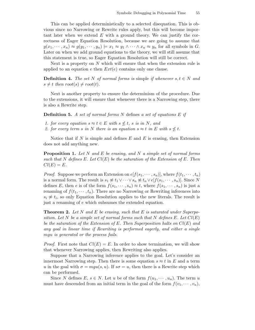
Symbolic Debugging in Polynomial Time 55
This can be applied deterministically to a selected disequation. This is ob-vious since no Narrowing or Rewrite rules apply, but this will become impor-tant later when we extend E with a ground theory. We can justify the cor-rectness of Eager Equation Resolution, because we are going to assume thatg(x1, · · · , xn) ≈ g(y1, · · · , yn) |= x1 ≈ y1 ∧ · · · ∧ xn ≈ yn for all symbols in G.Later on when we add ground equations to the theory, we will still assume thatthis statement is true, so Eager Equation Resolution will still be correct.
Next is a property on N which will ensure that when the extension rule isapplied to an equation e then Ext(e) contains only one clause.
Definition 4. The set N of normal forms is simple if whenever s, t ∈ N ands 6= t then root(s) 6= root(t).
Next is another property to ensure the determinism of the procedure. Dueto the extensions, it will ensure that whenever there is a Narrowing step, thereis also a Rewrite step.
Definition 5. A set of normal forms N defines a set of equations E if
1. for every equation s ≈ t ∈ E with s 6≤ t, s is in N , and2. for every term s in N there is an equation s ≈ t in E with s 6≤ t.
Notice that if N is simple and defines E and E is erasing, then Extensiondoes not add anything new.
Proposition 1. Let N and E be erasing, and N a simple set of normal formssuch that N defines E. Let Cl(E) be the saturation of the Extension of E. ThenCl(E) = E.
Proof. Suppose we perform an Extension on e[f(s1, · · · , sn)], where f(t1, · · · , tn)is a normal form. The result is s1 6≈ t1∨· · ·∨sn 6≈ tn∨e[f(s1, · · · , sn)]. Since Ndefines E, then e is of the form f(s1, · · · , sn) ≈ t, where f(s1, · · · , sn) is just arenaming of f(t1, · · · , tn). There are no Narrowing or Rewriting inferences intosi 6≈ ti, so only Equation Resolution applies to the new literals. The result isjust a renaming of e which subsumes the extended equation.
Theorem 2. Let N and E be erasing, such that E is saturated under Superpo-sition. Let N be a simple set of normal forms such that N defines E. Let Cl(E)be the saturation of the Extension of E. Then Superposition halts on Cl(E) andany goal in linear time if Rewriting is performed eagerly, and either a singlemgu is generated or the process fails.
Proof. First note that Cl(E) = E. In order to show termination, we will showthat whenever Narrowing applies, then Rewriting also applies.
Suppose that a Narrowing inference applies to the goal. Let’s consider aninnermost Narrowing step. Then there is some equation s ≈ t in E and a termu in the goal with σ = mgu(s, u). If sσ = u, then there is a Rewrite step whichcan be performed.
Since N defines E, s ∈ N . Let u be of the form f(u1, · · · , un). The term umust have descended from an initial term in the goal of the form f(v1, · · · , vn),

56 C. Lynch, B. Morawska
since E is erasing. Let θ be the accumulated substitution applied to the goal.Then ui ≈ viθ for each i. There also must have been an Extension at thebeginning where the disequations v1 6≈ w1 · · · vn 6≈ wn were added to the goal.These disequations were selected first in the goal, so we must have alreadyproved that viθ ≈ wiθ for all i. This implies that ui ≈ wiθ for all i.
Since we consider an innermost Narrowing step, ui must be reduced. Wealso know that wi is reduced, and there must be θ′ such that ui = wiθ
′ for alli. Therefore σ = θ′, and Rewriting can be applied.
Since we perform Eager Rewriting, this shows that no Narrowing steps willever be performed. Therefore, all inferences are deterministic. Every Rewritingstep applied to a term u in the goal will remove one occurrence of a symbol inF and replace it by symbols in G, since E is erasing.
Therefore, Rewriting will only be applied finitely many times, so the proce-dure will halt. Note that Equation Resolution does not increase the number ofsymbols of F appearing in the goal, as long as the goal is stored in a dag.
Since the result is don’t care nondeterministic, a single mgu will be gener-ated if the procedure halts.
Since each Rewriting removes a symbol of F from the goal, the total numberof applications of Rewriting is at most n, the size of the goal. If we apply eachunifier by representing the goal as a dag, then we can be sure that the set ofinferences do not grow the goal to be more than a constant times its originalsize, since each inference can only increase the size of the goal by a constantamount. And the number of Equation Resolution steps is just the number ofExtensions plus one, which is linear in the size of the goal. Since no Narrowingsteps are performed, the whole process is in linear time.
The example of List Theory L’ with the normal forms we have given iserasing, since there is only one normal form rooted with car and one normalform rooted with cdr. The set of normal forms N defines L’ because the set Nis just the set of left hand sides of L’. Furthermore, N and L’ is simple if welet F = car, cdr and let G = cons. Therefore, E-unification can be solvedin linear time for the theory of lists using Superposition with eager Rewriting,and the result will always be a most general unifier if it is solvable.
5 Lists with Length
It is possible to add some recursive theories and still run in polynomial time.Here we discuss a theory of Lists with Length. We extend the List theory toinclude the theory of length of lists.
length(nil) ≈ 0 length(cons(x, y)) = s(length(y))
The sort theory is extended to include:
L(nil) Int(length(xL)) Int(0) Int(s(xInt))
We could either make Int be the same type as the items of the list, or adifferent type.

Symbolic Debugging in Polynomial Time 57
This theory is difficult to handle, because many goals have an infinitecomplete set of unifiers. For example, the equation length(x) ≈ length(y)has infinitely many unifiers. The substitution [x 7→ y] is a unifier. But thenso is [x 7→ cons(x1, z), y 7→ cons(y1, z)], [x 7→ cons(x1, cons(x2, z)), [y 7→cons(y1, cons(y2, z))], etc. Normal forms will not help in this case. We haveto find a different solution if we want to find a halting procedure, much less apolynomial time procedure.
Our solution to this problem is to not allow any inferences into terms of theform length(x). Then we may not derive the empty clause of course. But, foreach goal, we will derive something from which we can tell whether or not thereis a solution. We will not give the entire complete set of unifiers. But we willgive a representation that should be meaningful to a programmer. For example,if we halt with length(x) ≈ length(y), then we suggest that this is even moremeaningful to a programmer than a schematization of the set of solutions.
The procedure for solving E-unification for lists with length is an extensionof the procedure for lists. We start by applying the extension rule to the orig-inal equations and goal. Then we run the Superposition procedure with eagerRewriting, and the following restriction:
The Superposition rule is restricted so that u is not allowed to be a term ofthe form length(x) with x a variable. Similarly, the Equation Resolution rule ismodified so that u and v may not contain any subterms of the form length(x)unless u or v is a variable. We add another rule to the inference system
cons(u1, u2) 6≈ cons(v1, v2) ∨ C
u1 6≈ v1 ∨ u1 6≈ v2 ∨ C
where cons(u1, u2) 6≈ cons(v1, v2) is selected. We will call this inference systemSuperposition with Length Restrictions.
After Superposition with Length Restrictions is performed, we fail if a dis-equation of the form cons(s, t) 6≈ nil appears in the leftover goal. Otherwise,we apply the inference system Syntactic Length Unification, which proceeds asfollows. We transpose the leftover goal clause C into a Syntactic Unificationproblem in the following way. We replace each term length(y) by a new vari-able xlength(y). Then we treat the clause like a set of equations, and performSyntactic Unification. If Syntactic Unification fails, then we fail. If syntacticunification succeeds, then we succeed. The answer substitution we get repre-sents a solution to the problem, but it is not really a substitution, because thelength(x) terms have been replaced by variables.
Note that after Superposition with Length Restrictions finishes, there areno car terms or cdr terms in the goal, because any well-sorted instance of thoseterms must contain a variable or a cons-term as a subterm, and we have shownin the previous section that all car or cdr terms will be rewritten. Also, afterSuperposition with Length Restrictions, there can be no cons terms left in thegoal. If a cons term appears directly underneath a car or cdr or length term,then it has been rewritten. This means that a cons symbol could only appear ina term where all nonvariable symbols are cons symbols. But then there must bean equation of the form s ≈ t where s contains only cons symbols and variables,and t is a length term or an s term or 0 or nil. If t is a length term or s term
58 C. Lynch, B. Morawska
or nil then the equation is not well-sorted, and we would have failed. If t is nilthen we would fail as described above. Therefore length must only be appliedto a variable, because length applied to an s term or 0 is not well-sorted, andlength(nil) would have been rewritten.
We need to prove that this process is sound and complete, and also that itruns in polynomial time.
Theorem 3. The inference system Superposition with Length restrictions fol-lowed by Syntactic Length Unification is sound and complete.
Proof. Since Superposition is sound and complete, that means that Superpo-sition with Length Restrictions preserves the set of solutions. So we need toprove that Syntactic Length Unification is sound and complete.
For completeness, we only need to show that Syntactic Length Unificationdoes not fail when there is a solution. If Syntactic Length Unification failsbecause of the clash rule, then Syntactic Unification (without transformationof length terms into variables) would fail also. So we only need to show thatfailures by Occurs Check are truly failures. Suppose we have an equation ofthe form xlength(y) ≈ t[xlength(y)], where xlength(y) is a proper subterm of t. Inorder to be well-sorted, xlength(y) must be an immediate subterm of s and smust be the root of the term or else immediately under another s, etc. Thisimplies that the occurs check must have occurred in an equation of the formxlength(y) = sn(xlength(y)) and we note that length(y) = sn(length(y)) has nosolution.
For soundness, we need to show that if our procedure succeeds, then therereally is a solution to the untransformed problem. Notice that if a variablexlength(y) appears, then y was given no substitution by Superposition withLength Restrictions. Furthermore y could not have appeared anywhere here ex-cept in the form length(y) because all car, cdr and cons have been removed, andsince y is of type list s(y) is not well-sorted. If y was one side of an equation, thenan Equation Resolution would have been performed. Therefore, y will be givenno value from Syntactic Length Unification. The only substitutions created bySyntactic Length Unification will be of the form xlength(y) = sn(xlength(z)) withn ≥ 0 or xlength(y) = sn(0) with n ≥ 0. Note that a variable cannot appearmore than once on a left hand side, or on both a left and right hand side. Toget a solution to the original problem, we could just let a variable z appearingon the right hand side be any list. In the first case above, y could be any listwith n more elements than z, and in the second case above y could be any listwith n elements.
Theorem 4. The inference system Superposition with Length restrictions fol-lowed by Syntactic Length Unification is don’t-care nondeterministic and runsin linear time.
Proof. The inference system is don’t-care nondeterministic because the twoindividual parts of it are. We have shown that whenever there is a Narrowinginvolving a car or cdr term then there is also a Rewriting. That is also the casefor length. If the argument is a cons term or nil then there is a Rewriting. If

Symbolic Debugging in Polynomial Time 59
the argument is a variable, then we have disallowed Narrowing. Therefore, thefirst part is don’t-care nondeterministic. The second part is too, because it isjust Syntactic Unification.
The first part runs in linear time, because there are no Narrowing infer-ences. All the Rewrite inferences will result in a term with fewer symbols. AndEquation Resolution won’t increase the size of the goal if it is kept in dag form.So the first part of the procedure is linear. The second part runs in linear timetoo, because Syntactic Unification does.
6 Extending Theory with Ground Equations
Now we extend a theory E with a ground theory. A ground set of equations canbe flattened so that every equation is of a flattened form, defined as follows.
Definition 6. A ground equation is flat if it is of the form
1. f(c1, · · · , cn) ≈ c, where c1, · · · , cn and c are constants, or
2. c ≈ d, where c and d are constants.
A set of ground equations is flat if every equation in the set is flat.
So in this section we will consider an original theory with signature Σ, whichwill also be the signature of the data structure theory E. Let ΣC be Σ extendedwith an infinite set of constants.
We begin with a set of equations E saturated under Superposition, with asignature Σ. We suppose that theory E is augmented with a flat set of groundequations S with signature ΣC . We want to give conditions under which E ∪Scan be finitely saturated under Superposition. We also want to find the condi-tions under which Superposition can solve E-unification problems for E ∪ S.
6.1 Automatic Decidability
Our first goal is to find conditions under which this extended theory can besaturated under Superposition. In order to show this for a particular theory,we can use the techniques of [1] automated in [3]. For example, for the theoryof Lists with Length, all initial ground equations are of the form car(a) ≈ b,cdr(a) ≈ b, cons(a, b) ≈ c, length(a) ≈ b, s(a) ≈ b or a ≈ b, where a, band c are constants. The only additional equations created by Superpositionare of the form s(length(a)) ≈ length(b) and length(a) ≈ s(b) where a and bare constants. This implies that Superposition can be performed in polynomialtime.
6.2 E-unification with Augmented Theory
Now we consider the problem of E-unification in the list theory L′ extended bya flat ground theory S. We allow S and the goal to contain symbols from L′
plus additional constants, but no other nonvariable symbols.

60 C. Lynch, B. Morawska
Theorem 5. Let L′ be the list theory with set of normal forms N . Let S be a setof flat ground equations. Let S′ be the saturation of E ∪ S. Then Superpositionwith the addition of Eager Equation Resolution halts on S′ in linear time forany goal if Rewriting is performed eagerly, and either a single mgu is generatedor the process fails.
Proof. The proof here is almost identical to the proof of Theorem 2. In thiscase, we can assume that Cl(E) = E, because if e cannot be inferred from anextension Ext(e) of a flat ground equation e, then e will not be able to be usedin the goal. So such equations e may be ignored.
Again, we just need to show that whenever Narrowing applies, Rewritingalso applies. We consider a Narrowing inference. First suppose it is an inferencewith car(cons(x, y)) ≈ x or cdr(cons(x, y)) ≈ y. Wlog, suppose it is the firstone. Then it Narrows into a term of the form car(z) or car(cons(z1, z2)). Bythe argument of Theorem 2, it cannot be a term of the form car(z), so it is aterm of the second form, and Rewriting is possible.
Next, suppose we Narrow with a term of the form car(a) ≈ b or cdr(a) ≈ b,where a and b are constants. Wlog, assume it is the first one. Then it must beNarrowing into a term of the form car(z) or car(a). We have already said thatit cannot be a term of the form car(z), so it must be a term of the form car(a),and then Rewriting applies.
All of the car and cdr symbols in a selected disequation will then be removedby eager Rewriting steps. At that point, the only nonvariable symbols left inthat disequation will be cons terms and constants. At that point, we apply EagerEquation Resolution. So all inferences steps are still don’t care nondeterministicor deterministic.
The procedure will still halt in a linear number of steps because all Rewritingsteps reduce the number of symbols in a term.
We stress the fact that S is not allowed to contain additional nonvariablesymbols that do not exist in E, except for constants, unless for such an extrasymbol h, we could conclude that h1(x1, · · · , xn) ≈ h(y1, · · · , yn) |= x1 ≈ y1 ∧· · · ∧ xn ≈ yn. For constants, this statement is trivial.
7 Conclusion
We have given a procedure for solving E unification problems in linear time, ifthe equational theory E meets certain conditions. The conditions imply that Eis closed under Paramodulation which implies that E-unification is in NP forthese theories[7, 4]. However it is difficult to get a polynomial time procedurefor such theories. To get this result, we needed to specify that some terms havea particular normal form.
Our result applies to the theory of lists, for example. Without our technique,Narrowing is exponential for the theory of lists. We also extended the techniqueto the theory of Lists plus Length. E-unification in that theory is not closedunder Paramodulation, but it has been shown to be decidable by [5]. The [5]result runs in exponential time, while ours is linear. We also showed how to get

Symbolic Debugging in Polynomial Time 61
a polynomial time procedure for E-unification modulo the theory of lists plusany ground theory.
Our results use the standard Superposition calculus, and do not need specialinference rules.
Our result is applicable to symbolic debugging problems, whereE-unificationis required to tell which values for variables determine a particular path throughthe program. Equations determine the conditions and assignment statements inthe program. For else statements, we need disequations too. Our results couldbe extended to cover that. It would also be interesting to consider all paths toa certain point in the program, not just particular paths.
References
1. A. Armando, S. Ranise and M. Rusinowitch. Uniform Derivation of Decision Proceduresby Superposition. In Proceedings 15th Workshop on Computer Science Logic., LNCS vol.2142, 513-527, 2001.
2. L. Bachmair and H. Ganzinger. Rewrite-based equational theorem proving with selectionand simplification. In Journal of Logic and Computation 4(3), 1-31, 1994.
3. C. Lynch and B. Morawska. Automatic Decidability. In Proceedings 17th IEEE Symposiumon Logic in Computer Science, LICS’02, IEEE Computer Society Press, 7-16, 2002.
4. C. Lynch and B. Morawska. Basic Syntactic Mutation. In Proceedings of Conference onAutomated Deduction (CADE), Vol. 2392 of LNAI, 471–485, 2002.
5. S. Mitra. Semantic Unification for Convergent Systems. Technical Report CS-R-94-1855,University of Illinois at Urbana-Champaign.
6. R. Nieuwenhuis. On Narrowing, Refutation Proofs and Constraints . In J. Hsiang, editor,6th International Conference on Rewriting Techniques and Applications (RTA) Springer-Verlag LNCS 914, pages 56-70, Kaiserslautern, Germany, April 4-7, 1995. Springer-Verlag.
7. R. Nieuwenhuis. Decidability and Complexity Analysis by Basic Paramodulation . Infor-mation and Computation, 147:1-21, 1998.
8. C. Weidenbach. Sorted Unification and Tree Automata in Bibel W. and Schmitt P. H.,editors, Automated Deduction - A Basis for Applications, Volume 1 of Applied Logic,Chapter 9, Kluwer, pp. 291-320, 1998
62 C. Lynch, B. Morawska

Combining Intruder Theories ⋆
Yannick Chevalier1 and Michael Rusinowitch2
1 IRIT Universite Paul Sabatier, Franceemail: [email protected]
2 LORIA – INRIA Lorraine, Franceemail: [email protected]
Abstract. Most of the decision procedures for symbolic analysis of proto-cols are limited to a fixed set of algebraic operators associated with a fixedintruder theory. Examples of such sets of operators comprise XOR, multipli-cation/exponentiation, abstract encryption/decryption. In this paper we givean algorithm for combining decision procedures for arbitrary intruder theorieswith disjoint sets of operators, provided that solvability of ordered intruderconstraints, a slight generalization of intruder constraints, can be decided ineach theory. This is the case for most of the intruder theories for which a de-cision procedure has been given. In particular our result allows us to decidetrace-based security properties of protocols that employ any combination of theabove mentionned operators with a bounded number of sessions.
1 Introduction
Recently many procedures have been proposed to decide insecurity of crypto-graphic protocols in the Dolev-Yao model w.r.t. a finite number of protocolsessions [2, 5, 19, 17]. Among the different approaches the symbolic ones [17, 10,4] are based on reducing the problem to constraint solving in a term algebra.This reduction has proved to be quite effective on standard benchmarks andalso was able to discover new flaws on several protocols [4].
However while most formal analysis of security protocols abstracts fromlow-level properties, i.e., certain algebraic properties of encryption, such as themultiplicativity of RSA or the properties induced by chaining methods for blockciphers, many real attacks and protocol weaknesses rely on these properties. Forattacks exploiting the XOR properties in the context of mobile communicationssee [7]. Also the specification of Just Fast Keying protocol (an alternative toIKE) in [1] employs a set constructor that is idempotent and commutative anda Diffie-Hellman exponentiation operator with the property (gy)z = (gz)y.
In this paper we present a general procedure for deciding security of pro-tocols in presence of algebraic properties. This procedure relies on the combi-nation of constraint solving algorithm for disjoint intruder theories, providedthat solvability of ordered intruder constraints, a slight generalization of in-truder constraints, can be decided in each theory. Such combination algorithmalready exists for solving E-unification problems [20, 3]. We have extended itin order to solve intruder constraints on disjoint signatures. This extension isnon trivial since intruder deduction rules allow one to build contexts aboveterms and therefore add some second-order features to the standard first-orderE-unification problem.
⋆ supported by IST AVISPA Project, ACI-SI SATIN, ACI-Jeune Chercheur
63

64 Y. Chevalier, M. Rusinowitch
Our approach is more modular than the previous ones and it allows usto decide interesting intruder theories that could not be considered before byreducing them to simpler and independant theories. For instance it allows oneto combine the exponentiation with abelian group theory of [18] with the Xortheory of [8].
Related works. Recently several protocol decision procedures have been de-signed for handling algebraic properties in the Dolev-Yao model [16, 6, 11, 8].These works have been concerned by fixed equational theories correspondingto a fixed intruder power. A couple of works only have tried to derive genericdecidability results for class of intruder theories. For instance, in [12] Delauneand Jacquemard consider the class of public collapsing theories. These theorieshave to be presented by rewrite systems where the right-hand side of every ruleis a ground term or a variable, which is a strong restriction.
2 Motivation
Combination of algebraic operators. We consider in this section the Need-ham-Schroeder Public-Key protocol. This well-known protocol is described inthe Alice and Bob notation by the following sequence of messages, where thecomma denotes a pairing of messages and MKa denotes the encryption bythe public key Ka of A.
A→ B : A,NaKb
B → A : Na, NbKa
A→ B : NbKb
Assume now that the encryption algorithm follows El-Gamal encryptionscheme. The public key of A is defined by three publicly-available parameters: amodulus pa, a base ga and the proper public key (ga)
a mod pa. The private keyof A is a. Denoting expp the exponentiation modulo p and ×p the multiplicationmodulo ϕ(p), and with new nonces k1, k2 and k3 we can rewrite the protocolas:
A→ B : exppb(gb, k1), (A,Na)⊕ exppb
(exppb(gb, b), k1)
B → A : exppa(ga, k2), (Na,Nb)⊕ exppa
(exppa(ga, a), k2)
A→ B : exppb(gb, k3), (Nb)⊕ exppb
(exppb(gb, b), k3)
In this simple example we would like to model the group properties of theExclusive-or (⊕), the associativity of exponential ((xy)z = xy×z), the groupproperty of the exponents. Several works have already been achieved toward tak-ing into account these algebraic properties for detecting attacks on a boundednumber of sessions. However none of these works can analyse protocols com-bining several algebraic operators like the example above. The algorithm givenin this paper will permit to decide the trace-based security properties of suchprotocols.Examples of intruder theories. A convenient way to specify intruder theo-ries in the context of cryptographic protocols is by giving a set L of deductionrules that tell how the intruder can construct new messages from the ones she

Combining Intruder Theories 65
already knows and a set of equational laws E that are verified by the functionsthat are employed in messages. We give here two examples of intruder theories.Some other theories are given in 6.
Abelian group theory. This intruder may treat messages as elements of anabelian group. We assume here there is only one such group and that the com-position law is · × ·, the inverse law is i(·) and the neutral element is denoted 1.
L×
→ 1x→ i(x)
x, y→ x× yE×
(x× y)× z = x× (y × z)x× y = y × x1× x = x
x× i(x) = 1
Dolev Yao with explicit destructors. The intruder is given with a pairingoperator and projections to retrieve the components of a pair. There is a sym-metric encryption operator se( , ) and an operator sd( , ) for the decryptionalgorithm too. For conciseness we omit the public-key encryption specification.
LDY
x, y → 〈x, y〉x→ π1(x)x→ π2(x)
x, y → se(x, y)x, y → sd(x, y)
EDY
π1(〈x, y〉) = xπ2(〈x, y〉) = y
sd(se(x, y), y) = x
3 Terms and subterms
We consider an infinite set of free constants C and an infinite set of variablesX . For all signatures G (i.e. a set of function symbols with arities), we denoteby T(G) (resp. T(G,X )) the set of terms over G ∪ C (resp. G ∪ C ∪ X ). Theformer is called the set of ground terms over G, while the later is simply calledthe set of terms over G. Variables are denoted by x, y, terms are denoted bys, t, u, v, and finite sets of terms are written E,F, ..., and decorations thereof,respectively. We abbreviate E∪F by E,F , the union E∪t by E, t and E \tby E \ t.
A constant is either a free constant or a function symbol of arity 0. Given aterm t we denote by Var(t) the set of variables occurring in t and by Cons(t) theset of constants occurring in t. We denote by Atoms(t) the set Var(t) ∪ Cons(t).We denote by A the set of all constants and variables. A substitution σ is aninvolutive mapping from X to T(G,X ) such that Supp(σ) = x|σ(x) 6= x, thesupport of σ, is a finite set. The application of a substitution σ to a term t (resp.a set of terms E) is denoted tσ (resp. Eσ) and is equal to the term t (resp. E)where all variables x have been replaced by the term xσ. A substitution σ isground w.r.t. G if the image of Supp(σ) is included in T(G).
In this paper, we consider 2 disjoint signatures F1 and F2, a consistentequational theory E1 (resp. E2) on F1 (resp. F2). We denote by F the union ofthe signatures F1 and F2, E the union of the theories E1 and E2. A term t inT(F1,X ) (resp. in T(F2,X )) is called a pure 1-term (resp. a pure 2-term).
The syntactic subterms of a term t are defined recursively as follows anddenoted Subsyn(t). If t is a variable or a constant then Subsyn(t) = t. If
66 Y. Chevalier, M. Rusinowitch
t = f(t1, . . . , tn) then Subsyn(t) = t ∪⋃n
i=1 Subsyn(ti). The positions in aterm t are defined recursively as usual (i.e. as sequences of integers), ǫ beingthe empty sequence. We denote by t|p the syntactic subterm of t at positionp. We denote by t[p ← s] the term obtained by replacing in t the syntacticsubterm t|p by s. We denote by Sign(·) the function that associates to eachterm t 6∈ C ∪ X the signature (F1, or F2) of its root symbol t|ǫ. For t ∈ C ∪ Xwe define Sign(t) = ⊥, with ⊥ a new symbol. The term s is alien to u ifSign(s) 6= Sign(u). Factors. We define the set of factors of a term t, and noteit Factors(t), the set of maximal syntactic subterms of t that are alien to t anddifferent of t. In particular Factors(t) = ∅ for t ∈ A.Subterms. We now define the notion of subterm values. Given a term t, theset of its subterm values is denoted by Sub(t) and is defined recursively by:Sub(t) = t ∪
⋃u∈Factors(t) Sub(u). For a set of terms E, Sub(E) is defined as
the union of the subterms values of the elements of E.
As an example consider F1 = ⊕, a, b, c and F2 = f where f has arity 1.Then Sub(a⊕ (b⊕ c)) = a⊕(b⊕c), a, b, c. On the other hand Sub(f(b⊕ c)) =f(b ⊕ c), b ⊕ c, b, c. This shows the difference with the notion of syntacticsubterms. In the rest of this paper and unless otherwise indicated, the notionof subterm will refer to subterm values.
Congruences and ordered rewriting. We shall introduce the notion of orderedrewriting [13], which is a useful tool that has been utilized (e.g. [3]) for provingthe correctness of combination of unification algorithms.
Let < be a simplification ordering on T(G) 3 assumed to be total on T(G)and such that the minimum for < is a constant cmin ∈ C. Given a possiblyinfinite set of equations O on the signature T(G) we define the ordered rewritingrelation →O by s →O s′ iff there exists a position p in s, an equation l = r inO and a substitution τ such that s = s[p← lτ ], s′ = s[p← rτ ], and lτ > rτ .
It has been shown (see [13]) that by applying the unfailing completion pro-cedure [15] to a set of equations H we can derive a (possibly infinite) set ofequations O such that:
1. the congruence relations =O and =H are equal on T(F).
2. →O is convergent (i.e. terminating and confluent) on T(F).
We shall say that O is an o-completion of H.
The relation →O being convergent on ground terms we can define (t)↓O asthe unique normal form of the ground term t for →O. Given a ground substi-tution σ we denote by (σ)↓O the substitution with the same support such thatfor all variables x ∈ Supp(σ) we have x(σ)↓O = (xσ)↓O. A substitution σ isnormal if σ = (σ)↓O.
We will denote by R an o-completion of E = E1∪E2. We denote by Cspe theset containing the constants in F and cmin.
3 by definition < satisfies for all s, t, u ∈ T(G) s < t[s] and s < u implies t[s] < t[u]
Combining Intruder Theories 67
4 Protocols, intruders and constraint systems
Security of a given protocol is assessed with respect to a class of environments inwhich the protocol is executed. Dolev and Yao have described the environmentnot in terms of possible attacks on the protocol but by the deduction an intruderattacking a protocol execution is able to perform.
In Subsection 4.1 we define an extension of Dolev-Yao model to arbitraryoperators for modeling the possible deductions of the intruder. In Subsection 4.2we define the protocol semantics for an execution within an hostile environmentcontrolled by the intruder and in Subsection 4.3 we describe how we representthis execution by a constraint system.
4.1 Intruder deduction systems
We shall model messages as ground terms and intruders deduction rules asrewrite rules on sets of messages representing the knowledge of an intruder. Theintruder derives new messages from a given (finite) set of messages by applyingintruder rules. Since we assume some equational axioms H are satisfied byfunctions symbols in the signature, all these derivations have to be consideredmodulo the equational congruence =H generated by these axioms.
An intruder deduction rule in our setting is specified by a term t in somesignature G. Given values for the variables of t the intruder is able to generatethe corresponding instance of t.
Definition 1. An intruder system I is given by a triple 〈G, T,H〉 where G isa signature, T ⊆ T(G,X ) and H is a set of axioms between terms in T(G,X ).To each t ∈ T we associate a deduction rule Lt : Var(t) → t and Lt,g denotesthe set of ground instances of the rule Lt:
Lt,g = l→ r | ∃σ, ground substitution on G, l = Var(t)σ and r =H tσ
The set of rules LI is defined as the union of the sets Lt,g for all t ∈ T .
Each rule l → r in LI defines an intruder deduction relation →l→r betweenfinite sets of terms. Given two finite sets of terms E and F we define E →l→r Fif and only if l ⊆ E and F = E ∪ r. We denote →I the union of the relations→l→r for all l → r in LI and by →∗
I the transitive closure of →I . We simplydenote by → the relation →I when there is no ambiguity about I.
For instance we can define I× = 〈×, i, 1, x× y, i(x), 1, E×〉 and we havea, b, c→I× a, b, c, c × a.
A derivation D of length n, n ≥ 0, is a sequence of steps of the formE0 →I E0, t1 →I · · · →I En with finite sets of ground terms E0, . . . En, andground terms t1, . . . , tn, such that Ei = Ei−1 ∪ ti for every i ∈ 1, . . . , n.
The term tn is called the goal of the derivation. We define EI
to be equal tothe set t | ∃F s.t. E →∗
I F and t ∈ F i.e. the set of terms that can be derivedfrom E. If there is no ambiguity on the deduction system I we write E instead
of EI.

68 Y. Chevalier, M. Rusinowitch
Let O be an o-completion of H. We will assume from now that all thededuction rules generate terms that are normalized by →O and the goal andthe initial set are in normal form for →O. It can be shown [9] that this is notrestrictive for our main decidability result.
Given a set of terms T ⊆ T(G,X ) we define the set of terms 〈T 〉 to be theminimal set such that T ⊆ 〈T 〉 and for all t ∈ 〈T 〉 and for all substitutions σwith image included in 〈T 〉, we have tσ ∈ 〈T 〉. Hence terms in 〈T 〉 are built bycomposing terms in T iteratively. We can prove easily that the intruder systemsI = 〈G, T,H〉 and J = 〈G, 〈T 〉 ,H〉 define the same sets of derivable terms, i.e.
for all E we have EI
= EJ
.
We want to consider now the union of 2 intruder systems: I1 = 〈F1, T1, E1〉and I2 = 〈F2, T2, E2〉. In particular we are interested in the derivations obtainedby using →I1 ∪ →I2. It can be noticed that 〈T1 ∪ T2〉 = 〈〈T1〉 ∪ 〈T2〉〉. Henceby the remarks above the derivable terms using 〈T1 ∪ T2〉 or 〈T1〉 ∪ 〈T2〉 arethe same. For technical reason it will be more convenient to use 〈T1〉 ∪ 〈T2〉 fordefining the union of 2 intruder systems:
Definition 2. The union of the two intruder systems 〈F1, T1, E1〉 , 〈F2, T2, E2〉is the intruder system U = 〈F1 ∪ F2, 〈T1〉 ∪ 〈T2〉 , E1 ∪ E2〉.
A derivation E0 →U E0, t1 →U · · · →U En of intruder system U is well-formed if for all i ∈ 1, . . . , n we have ti ∈ Sub(E0, tn); in other words everymessage generated by an intermediate step either occurs in the goal or in the ini-tial set of messages. In the following lemma the derivations refer to the intrudersystem U = 〈F1 ∪ F2, 〈T1〉 ∪ 〈T2〉 , E1 ∪ E2〉. For the proof see [9]:
Lemma 1. A derivation of minimal length starting from E of goal t is well-formed.
4.2 Protocol analysis
In this subsection we describe how protocols are modelled. In the following weonly model a single session of the protocol since it is well-known how to reduceseveral sessions to this case. Our semantics follows the one by [12].
In Dolev-Yao model the intruder has complete control over the commu-nication medium. We model this by considering the intruder is the network.Messages sent by honest agents are sent directly to the intruder and messagesreceived by the honest agents are always sent by the intruder. From the intruderside a finite execution of a protocol is the interleaving of a finite sequence ofmessages it has to send and a finite sequence of messages it receives (and addto its knowledge).
We also assume that the interaction of the intruder with one agent is anatomic step. The intruder sends a message m to an honest agent, this agenttests the validity of this message and responds to it. Alternatively an agentmay initiate an execution and in this case we assume it reacts to a dummymessage sent by the intruder.
A step is a triplet (recv(x); send(s);cond(e)) where x ∈ X , s ∈ T(G,X )and e is a set of equations between terms of T(G,X ). The meaning of a step is

Combining Intruder Theories 69
that upon receiving message x, the honest agent checks the equations in e andsends the message s. An execution of a protocol is a finite sequence of steps.
Example 1. Consider the following simple protocol:
A→ B : M ⊕BKB → A : BA→ B : KB → A : M
Assuming the algebraic properties of ⊕, symmetric encryption se(, ) and sym-metric decryption sd(, ) we model this protocol as:
recv(v1); send(se(M ⊕B,K));cond(v1 = cmin)recv(v2); send(B);cond(∅)recv(v3); send(K);cond(v3 = B)recv(v4); send(sd(v2, v4)⊕B);cond(v4 = K)recv(v5); send(cmin);cond(v5 = M)
Note that in our setting we can model that at some step i the message must
match the pattern ti by adding an equation vi?= ti to S.
In order to define whether an execution of a protocol is feasible we mustfirst define when a substitution σ satisfies a set of equations S.
Definition 3. (Unification systems) Let H be a set of axioms on T(G,X ). An
H-Unification system S is a finite set of equations in T(G,X )denoted by (ui?=
vi)i∈1,...,n. It is satisfied by a ground substitution σ, and we note σ |= S, if forall i ∈ 1, . . . , n uiσ =H viσ.
Let I=〈G, T,H〉 be an intruder system. A configuration is a couple 〈P,N〉where P is a finite sequence of steps and N is a set of ground terms (the knowl-edge of the intruder). From the configuration 〈(recv(x); send(s);cond(e)) ·P,N〉 a transition to (P ′, N ′) is possible iff there exists a ground substitution σ
such that xσ ∈ NI, σ |= e, N ′ = N ∪ sσ and P ′ = Pσ. Trace based-security
properties like secrecy can be reduced to the following Execution feasabilityproblem.
Execution feasability
Input: an initial configuration 〈P,N0〉Output: SAT iff there exists a reachable configuration 〈∅,M〉
4.3 Constraints systems
We express the execution feasability of a protocol by a constraint problem C.
Definition 4. (Constraint systems) Let I = 〈G, T,H〉 be an intruder system.An I-Constraint system C is denoted: ((Ei ⊲ vi)i∈1,...,n,S) and it is definedby a sequence of couples (Ei, vi)i∈1,...,n with vi ∈ X and Ei ⊆ T(G) for i ∈1, . . . , n and Ei−1 ⊆ Ei for i ∈ 2, . . . , n and by an H-unification system S.
An I-Constraint system C is satisfied by a ground substitution σ if for alli ∈ 1, . . . , n we have viσ ∈ Eiσ and if σ |= S. If a ground substitution σsatisfies a constraint system C we denote it by σ |=I C.
70 Y. Chevalier, M. Rusinowitch
Constraint systems are denoted by C and decorations thereof. Note that if asubstitution σ is a solution of a constraint system C, by definition of constraintsand of unification systems the substitution (σ)↓O is also a solution of C (whereOis an o-completion of H). In the context of cryptographic protocols the inclusionEi−1 ⊆ Ei means that the knowledge of an intruder does not decrease as theprotocol progresses: after receiving a message an honest agent will respond toit. This response can be added to the knowledge of an intruder who listens allcommunications.
Example 2. We model the protocol of Example 1 by the following constraintsystem. First we gather all conditions in an unification system S
S =v1
?= cmin , v3
?= B , v4
?= K , v5
?= M
The protocol execution for intruder I with initial knowledge cmin is thenexpressed by the constraint:
C = (( cmin ⊲ v1,cmin, se(M ⊕B,K) ⊲ v2,cmin, se(M ⊕B,K), B ⊲ v3,cmin, se(M ⊕B,K), B,K ⊲ v4),cmin, se(M ⊕B,K), B,K, sd(v2, v4)⊕B ⊲ v5,S)
We are not interested in general constraint systems but only in those relatedto protocols. In particular we need to express that a message to be sent atsome step i should be built from previously received messages recorded in thevariables vj , j < i, and from the initial knowledge. To this end we define:
Definition 5. (Deterministic Constraint Systems) An I-constraint system((Ei⊲vi)i∈1,...,n,S) is deterministic if for all i ∈ 1, . . . , n we have Var(Ei) ⊆v1, . . . , vi−1
The decision problems we are interested in are the satisfiability and theordered satisfiability of intruder constraint systems.
Satisfiability
Input: an I-constraint system COutput: Sat iff there exists a substitution σ such that: σ |=I C.
In order to be able to combine solutions of constraints in component theoriesto get a solution for the full theory these solutions have to satisfy some orderingconstraints too. Intuitively, this is to avoid introducing cycle when building aglobal solution. This motivates the following definition:
Ordered Satisfiability
Input: an I-constraint system C, X the set of all variables and C theset of all free constants occurring in C and a linear ordering ≺on X ∪ C.
Combining Intruder Theories 71
Output: Sat iff there exists a substitution σ such that:σ |=I C∀x ∈ X and ∀c ∈ C, x ≺ c implies c /∈ Subsyn(xσ)
The main result of this paper is the following modularity result:
Theorem 1. If the ordered satisfiability problem is decidable for two intruders〈F1, T1, E1〉 and 〈F2, T2, E2〉 for disjoint signatures F1 and F2 then the satisfia-bility problem is decidable for the intruder U = 〈F1 ∪ F2, 〈T1〉 ∪ 〈T2〉 , E1 ∪ E2〉.
This result is obtained as a direct consequence of the next section where wegive an algorithm for solving U -constraints using algorithms for solving orderedsatisfiability for intruders 〈F1, T1, E1〉 and 〈F2, T2, E2〉.
5 Combination of decision procedures
We introduce Algorithm 1 for solving satisfiability of constraint systems for theunion U of two intruders systems I1 = 〈F1, T1, E1〉 and I2 = 〈F2, T2, E2〉 withdisjoint signatures F1 and F2. The completeness of Algorithm 1 is sketchedbelow, and the proofs (for completeness and soundness) are fully detailed in [9].Let us explain this algorithm:Step 2 The algorithm input is a U -Constraint system (D,S). An equational
system S is homogeneous if for all u?= v ∈ S, u and v are both pure 1-terms
or both pure 2-terms. It is well-known that equational systems can be trans-formed into equivalent (w.r.t. satisfiability) homonogeneous systems. Thus wecan assume that S is homogeneous without loss of generality.Step 3 abstracts every subterm t of C by a new variable ψ(t). A choice of ψsuch that ψ(t) = ψ(t′) will lead to solutions that identify t and t′.Steps 4-6 assign non-deterministically a signature to the root symbol of thesubterms of C instanciated by a solution. The choice th(ψ(t)) = 0 correspondsto the situation where t gets equal to a free constant.Steps 7-10 choose and order non-deterministically the intermediate subtermsin derivations that witness that the solution satisfies the constraints in D.Step 11 defines a constraint problem C′ collecting the previous choices on sub-terms identification, subterms signatures and derivation structures.Step 12 splits the problem S ′ in two pure subproblems.Step 13 splits non-deterministically the problem D′, that is we select for eachE ⊲ v in D′ an intruder system to solve it.Step 14 guesses an ordering on variables: this ordering will preclude the valueof a variable from being a subterm of the value of a smaller variable. This isused to avoid cycles in the construction of the solution.Step 15 solves independantly the 2 pure subproblems obtained at steps 12-13.In Ci the variables q with th(q) 6= i will be considered as constants.
We assume Cspe ⊆ Sub(C). Recall that R is the rewrite system associatedto E = E1 ∪ E2. We say a normal substitution σ is bound if for all variables xwith xσ 6= x and for all t ∈ Sub(xσ) there exists u ∈ Sub(C) ∪ Cspe such that(uσ)↓R = t. A key proposition is:

72 Y. Chevalier, M. Rusinowitch
Algorithm 1 Combination Algorithm1: SolveU(C)2: Let C = ((Ei ⊲ vi)i∈1,...,n,S) with S homogeneous.3: Choose ψ an application from Sub(C) to X \ Var(C)
and let Q = ψ(Sub(C))4: for all q ∈ Q do
5: Choose a theory th(q) ∈ 0, 1, 26: end for
7: for i = 1 to n do
8: Choose Qi ⊆ Q
9: Choose a linear ordering over the elements of Qi say (qi,1, . . . , qi,ki)
10: end for
11: Let C′ = (D′,S ′) where
(
S ′ = S ∪n
z?= ψ(z) | z ∈ Sub(C)
o
D′ = ∆1, . . . ,∆i, . . .∆n
and ∆i = (Ki, Q<ji ⊲ qi,j)j∈1,...,ki, (Ki, Qi ⊲ ψ(vi)) with
Ki = ψ(Ei) ∪Si−1
j=1Qj
Q<ji = qi,1, qi,2, . . . , qi,j−1
12: Split S ′ into S1,S2 such that S ′ = S1 ∪ S2 and:
8
<
:
S1 =n
z?= z′ ∈ S ′ | z, z′are pure 1-terms
o
S2 =n
z?= z′ ∈ S ′ | z, z′are pure 2-terms
o
13: Split non-deterministically D′ into D1,D2
14: Choose a linear ordering ≺ over Q.15: Solve Ci = (Di,Si) for intruder Ii with linear ordering ≺ for i ∈ 1, 216: if both are satisfied then
17: Output: Satisfied18: end if
Proposition 1. If C is a satisfiable constraint system there exists a bound sub-stitution σ such that σ |= C. Moreover Sub((Sub(C)σ)↓R) = (Sub(C)σ)↓R∪Cspe.
5.1 Completeness of the algorithm
Proposition 2. If C is satisfiable then there exists C1 and C2 satisfiable atStep 15 of the algorithm.
Proof. First let us prove that the 11 first steps of the algorithm preserve satis-fiability. Assume C is satisfiable. By Proposition 1 there exists a normal boundsubstitution σ which satisfies C. Define ψ to be a function from Sub(C) to a setof variables Q such that ψ(t) = ψ(t′) if and only if (tσ)↓R = (t′σ)↓R. Thus byProposition 1 there exists a bijection φ from Q to Sub((Sub(C)σ)↓R). We letth(q) = i if Sign(φ(q)) = Fi and th(q) = 0 if Sign(φ(q)) = ⊥. By the construc-tion of S ′ and the choice of ψ we can extend σ on Q by qσ = (ψ−1(q)σ)↓R.
For each i ∈ 1, . . . , n by Lemma 1 we can consider a well-formed derivationDi starting from Fi = (Eiσ)↓R and of goal gi = viσ:
Di : Fi →U Fi, ri,1 →U · · · →U Fi, ri,1, . . . , ri,ki→U Fi, ri,1, . . . , ri,ki
, gi

Combining Intruder Theories 73
We have Sub(Fi, gi) ⊆ Sub((Sub(Cσ))↓R). Since the derivation is well-formedwe have ri,1, . . . , ri,ki
⊆ Sub(Fi, gi). By Proposition 1, Sub((Sub(Cσ))↓R) =(Sub(Cσ))↓R Thus the function φ−1 is defined for each ri,j . Let qi,j = φ−1(ri,j)and Qi be the sequence of the qi,j.
The algorithm will non-deterministically produce a C′ corresponding to thesechoices and satisfied by σ (extended over Q by ψ(t)σ = (tσ)↓R) by construction.Since S is satisfiable, following the lines of F. Baader and K. Schulz [3] permitsto prove that S1 and S2 are satisfiable with a linear constant restriction ≺chosen such that q ≺ q′ implies q′σ is not a subterm of qσ.
We choose the sequence of constraints in D1 (resp. D2) to be the subsequenceof constraints F ⊲ q from D′ such that the corresponding transition in thesolution was performed by a rule in Lu,g with Sign(u) = F1 (resp. F2). Byconstruction these two systems are satisfiable.
From the soundness and completeness of Algorithm 1 and the (non trivial)fact that the constraint Ci = (Di,Si) can be chosen to be deterministic, we canderive our main result on the combination of two intruders. It can be easilygeneralized to n intruders over disjoint signatures F1, . . . ,Fn.
6 Application to Security Protocols
In order to combine constraint solving algorithms for subtheories we only needto show that ordered satisfiability is decidable in each component theory. Toillustrate the benefit of our approach we show that this is the case for severaltheories encoding useful properties of cryptographic primitives (pair, xor, expo-nential, encryption). A consequence of our main result Theorem 1 is that we candecide the security of (finite sessions of) any protocol employing these primi-tives even assuming their algebraic properties and even if they are employedall together.
6.1 Abelian group operators
We consider in this subsection the case of an intruder I× = 〈F×, S×, E×〉, whereF× is the signature i(·), · × ·, 1, T× is the set of terms i(x), x × y, 1 and withthe equational theory:
E×
(x× y)× z = x× (y × z)x× y = y × x1× x = x
x× i(x) = 1
We reduce decidability of I×-constraints to satisfiability of affine systems ofequations on Z. This reduction is performed in two steps. First we prove thatit suffices to consider ground sets Ei in the constraints, and thus that the vi arelinear combination of ground terms. Second the unification system is translatedto a system of affine equations over Z.
Lemma 2. One can compute C′ = ((E′i ⊲ vi)i∈1,...,n,S) from C such that
74 Y. Chevalier, M. Rusinowitch
– σ |= C iff σ |= C′
– for all i ∈ 1, . . . , n the set E′i is ground
This leads to next proposition.
Proposition 3. The ordered satisfiability problem for deterministic constraintsand intruder I× is decidable in NPTIME.
6.2 XOR operator
We consider the intruder I⊕ = 〈F⊕, x⊕ y, 0, E⊕〉 with the signature F⊕ =0, · ⊕ · and with equational theory:
E⊕
(x⊕ y)⊕ z = x⊕ (y ⊕ z)x⊕ y = y ⊕ x0⊕ x = xx⊕ x = 0
Let C = ((Ei ⊲ vi)i∈1,...,n,S) be a deterministic constraint problem forI⊕. Lemma 2 can be adapted to this case. The main difference is that affinesystems are over (Z/2Z). We refer to [14] for a more detailed description of thetranslation from unification problems to linear systems and of the resolution ofsuch systems.
Proposition 4. The ordered satisfiability problem for deterministic constraintsand intruder I⊕ is decidable in PTIME.
6.3 Exponential operator
For simplicity of exposition we assume that all exponentiations are computedin the same modulus.
Let Fexp = exp(·, ·), i(·), · × · and Texp = x× y, exp(x, y), exp(x, i(y)).We now consider the intruder system Iexp = 〈Fexp, Texp, Eexp〉 where
Eexp
exp(x, 1) = xexp(exp(x, y), z) = exp(x, y × z)
(x× y)× z = x× (y × z)x× y = y × x1× x = x
x× i(x) = 1
Following [18] the satisfiability problem for deterministic constraint systemsfor this intruder can be reduced to the satisfiability problem for an abelian groupoperator. We can deduce:
Proposition 5. The ordered satisfiability problem for deterministic constraintsand intruder Iexp is decidable in NPTIME.
Combining Intruder Theories 75
6.4 Equational Dolev-Yao theory with explicit decryption
We consider now the Dolev-Yao intruder IDY = 〈FDY , TDY , EDY 〉 over the sig-nature FDY = 〈·, ·〉 , π1(·), π2(·), se(·, ·), sd(·, ·) with deduction system definedby SDY = 〈x, y〉 , π1(x), π2(x), se(x, y), sd(x, y) and the equational theory:
EDY
π1(〈x, y〉) = xπ2(〈x, y〉) = y
sd(se(x, y), y) = x
First we note that we can get from EDY a convergent and finite rewrite sys-tem RDY simply by orienting the axioms from left to right. Thanks to Theorem8.5. of Schmidt-Schauss [20] satisfiability of equational systems modulo EDY isdecidable even in presence of linear constant restrictions. The idea is that theso-called narrowing procedure modulo RDY terminates (since rules right-handsides are variables) and is complete for solving equations modulo EDY withlinear constant restrictions.
The algorithm of [2] for deciding intruder IDY -constraints can be adaptedto generate a finite and complete set of symbolic solutions. Then we can use theconstant elimination technique of [20] to solve the ordered satisfiability problem:we apply narrowing (i.e. instanciating and rewriting) to the complete set ofsymbolic solutions provided by [2] and then we eliminate from the resultingsubstitutions the ones that do not satisfy the constant restrictions.
7 Conclusion
We have proposed an algorithm for combining decision procedures for intruderconstraints on disjoint signatures. This algorithm allows for a modular treat-ment of algebraic operators in protocol analysis and a better understanding ofcomplexity issues in the domain. Since only constraint satisfiability is requiredfrom the intruder subtheories the approach should permit one to handle morecomplex operators.
References
1. M. Abadi, B. Blanchet, and C. Fournet. Just Fast Keying in the Pi Calculus. In DavidSchmidt, editor, Proceedings of ESOP’04, volume 2986 of Lecture Notes on ComputerScience, pages 340–354, Barcelona, Spain, 2004. Springer Verlag.
2. R. Amadio, D. Lugiez, and V. Vanackere. On the symbolic reduction of processes withcryptographic functions. Theor. Comput. Sci., 290(1):695–740, 2003.
3. F. Baader and K. U. Schulz. Unification in the union of disjoint equational theories.combining decision procedures. J. Symb. Comput., 21(2):211–243, 1996.
4. D. Basin, S. Modersheim, and L. Vigano. An On-The-Fly Model-Checker for SecurityProtocol Analysis. In Einar Snekkenes and Dieter Gollmann, editors, Proceedings ofESORICS’03, LNCS 2808, pages 253–270. Springer-Verlag, 2003.
5. M. Boreale. Symbolic trace analysis of cryptographic protocols. In Proceedings of the 28thICALP’01, LNCS 2076, pages 667–681. Springer-Verlag, Berlin, 2001.
6. M. Boreale and M. Buscemi. Symbolic analysis of crypto-protocols based on modularexponentiation. In Proceedings of MFCS 2003, volume 2747 of Lecture Notes in ComputerScience. Springer, 2003.

76 Y. Chevalier, M. Rusinowitch
7. N. Borisov, I. Goldberg, and D. Wagner. Intercepting mobile communications: the inse-curity of 802.11. In Proceedings of MOBICOM 2001, pages 180–189, 2001.
8. Y. Chevalier, R. Kuesters, M. Rusinowitch, and M. Turuani. An NP Decision Procedurefor Protocol Insecurity with XOR. In Proceedings of the Logic In Computer ScienceConference, LICS’03, June 2003.
9. Y. Chevalier and M. Rusinowitch. Combining intruder theories. Technical report, INRIA,2005. http://www.inria.fr/rrrt/liste-2005.html.
10. Y. Chevalier and L. Vigneron. A Tool for Lazy Verification of Security Protocols. In Pro-ceedings of the Automated Software Engineering Conference (ASE’01). IEEE ComputerSociety Press, 2001.
11. H. Comon-Lundh and V. Shmatikov. Intruder Deductions, Constraint Solving and In-security Decision in Presence of Exclusive or. In Proceedings of the Logic In ComputerScience Conference, LICS’03, pages 271–280, 2003.
12. S. Delaune and F. Jacquemard. A decision procedure for the verification of securityprotocols with explicit destructors. In Proceedings of the 11th ACM Conference on Com-puter and Communications Security (CCS’04), pages 278–287, Washington, D.C., USA,October 2004. ACM Press.
13. N. Dershowitz and J-P. Jouannaud. Rewrite systems. In Handbook of Theoretical Com-puter Science, Volume B, pages 243–320. Elsevier, 1990.
14. G. Guo, P. Narendran, and D. A. Wolfram. Unification and matching modulo nilpotence.Information and Computation, 162((1-2)):3–23, 2000.
15. J. Hsiang and M. Rusinowitch. On word problems in equational theories. In ICALP,volume 267 of Lecture Notes in Computer Science, pages 54–71. Springer, 1987.
16. C. Meadows and P. Narendran. A unification algorithm for the group Diffie-Hellmanprotocol. In Workshop on Issues in the Theory of Security (in conjunction with POPL’02),Portland, Oregon, USA, January 14-15, 2002.
17. J. Millen and V. Shmatikov. Constraint solving for bounded-process cryptographic pro-tocol analysis. In ACM Conference on Computer and Communications Security, pages166–175, 2001.
18. J. Millen and V. Shmatikov. Symbolic protocol analysis with an abelian group operatoror Diffie-Hellman exponentiation. Journal of Computer Security, 2005.
19. M. Rusinowitch and M. Turuani. Protocol insecurity with finite number of sessions is NP-complete. In Proc.14th IEEE Computer Security Foundations Workshop, Cape Breton,Nova Scotia, June 2001.
20. M. Schmidt-Schauß. Unification in a combination of arbitrary disjoint equational theories.J. Symb. Comput., 8(1/2):51–99, 1989.

Can Context Sequence Matching Be Usedfor XML Querying?⋆
Temur Kutsia1 and Mircea Marin2
1 Research Institute for Symbolic ComputationJohannes Kepler University
A-4040 Linz, [email protected]
2 Graduate School of Systems and Information EngineeringUniversity of Tsukuba
Tsukuba 305-8573, [email protected]
Abstract. We describe a matching algorithm for terms built over flexible arityfunction symbols and context, function, sequence, and individual variables. Thealgorithm is called a context sequence matching algorithm. Context variablesallow matching to descend in term-trees to arbitrary depth. Sequence variablesallow matching to move in term-trees in arbitrary breadth. The ability to exploreterms in two orthogonal directions in a uniform way may be useful for queryingdata available as a large term, like XML documents. We extend the algorithm toprocess regular constraints and discuss its possible application in XML querying.
1 Introduction
We describe a context sequence matching algorithm and discuss its possibleapplication in querying XML [27]. Context variables may be instantiated witha context—a term with a hole. They permit matching to descend to arbitrarydepth in a term represented as a tree. Sequence variables may be instanti-ated with a finite (maybe empty) sequence of terms. They are normally usedwith flexible arity function symbols and permit matching to move to arbitrarybreadth. Thus, context and sequence variables together allow exploring termsin two orthogonal directions in a uniform way which may be useful for queryingdata available as a large term, like XML documents.
Besides context and sequence variables we have function and individual vari-ables. Function variables may be instantiated with a single function symbol orwith another function variable. Individual variables may be bound with a singleterm. Like context and sequence variables, functional and individual variablescan be used to traverse terms in depth and breadth, respectively, but only inone level.
In this paper first we describe a minimal and complete rule-based algorithmfor context sequence matching. It operates on terms built using flexible ar-ity function symbols and involving context, sequence, function, and individualvariables. Then we show how to use context sequence matching in a declarativeXML query language. At the end, we extend the algorithm to deal with regular
⋆ Temur Kutsia has been supported by the Austrian Science Foundation (FWF) underProject SFB F1302 and F1322.
77
78 T. Kutsia, M. Marin
constraints, both in depth and in breadth. Context sequence matching, with orwithout regular restrictions, is finitary. Regular expressions provide a powerfulmechanism for restricting data values in XML. Many languages have supportfor them.
Context matching and unification have been intensively investigated in therecent past years, see e.g, [9, 10, 20, 24–26]. Context matching is decidable. De-cidability of context unification is still an open question. Schmidt-Schauß andStuber in [26] gave a context matching algorithm and noted that it can be usedsimilar to XPath [7] matching for XML documents. Sequence matching and uni-fication was addressed, for instance, in [2, 12, 13, 16–18, 22]. Both matching andunification with sequence variables are decidable. Sequence unification proce-dure described in [17, 18] was implemented in the constraint logic programminglanguage CLP(Flex) [8] and was used for XML processing.
Simulation unification [4] implemented in the Xcerpt language has a ‘descen-dant’ construct that is similar to context variables in the sense that it allowsto descend in terms to arbitrary depth, but it does not allow regular expres-sions along it. Also, sequence variables are not present there. However, it canprocess unordered and incomplete queries, and it is a full scale unification, nota matching. Having sequence variables in a full scale unification would make itinfinitary (see e.g., [18]).
In our opinion, context sequence matching can serve as a computationalmechanism for a declarative, rule-based language to query and transform XML.Such a query language would have advantages of both path-based and pattern-based languages that form two important classes of XML query languages. Path-based languages usually allow to access a single set of nodes of the graph or treerepresenting an XML data. The access is based on relations with other nodesin the graph or tree specified in the path expression. Pattern-based languagesallow access to several parts of the graph or tree at once specifying the relationsamong the accessed nodes by tree or graph patterns. (For a recent survey overquery and transformation languages see [11].) Moreover, with context sequencematching we can achieve improved control on rewriting that can be useful forrewriting-based web site specification and verification techniques [1]. In ouropinion, a system like ρLog [23] can be extended to a prototype of such a querylanguage. ρLog is a rule-based language whose computational mechanism usessequence matching with function variables. It supports single and multiple queryanswers, non-deterministic computations, and has a clean declarative semantics.However, implementation issues for such a query language is not a subject ofthis paper.
Another possible application area for context sequence matching is math-ematical knowledge management. For instance, it can retrieve algorithms orproblems from the schema library [5] of the Theorema system [6].
The results of this paper extend those of [19] by considering regular expres-sions on full contexts instead of functions only.
The paper is organized as follows: In Section 2 we introduce preliminarynotions. In Section 3 we describe the context sequence matching algorithm. Itsapplication in XML querying is discussed in Section 4. Section 5 is about regularexpression matching for context and sequence variables. Section 6 concludes.
Can Context Sequence Matching Be Used for XML Querying? 79
2 Preliminaries
We assume fixed pairwise disjoint sets of symbols: individual variables VInd,sequence variables VSeq, function variables VFun, context variables VCon, andfunction symbols F . The sets VInd, VSeq, VFun, and VCon are countable. Theset F is finite or countable. All the symbols in F except a distinguished con-stant (called a hole) have flexible arity. We will use x, y, z for individualvariables, x, y, z for sequence variables, F,G,H for function variables, C,D,Efor context variables, and a, b, c, f, g, h for function symbols. We may use thesemeta-variables with indices as well.
Terms are constructed using the following grammar:
t ::= x | x | | f(t1, . . . , tn) | F (t1, . . . , tn) | C(t)
In C(t) the term t can not be a sequence variable. We will write a for theterm a() where a ∈ F . The meta-variables s, t, r, maybe with indices, will beused for terms. A ground term is a term without variables. A context is a termwith a single occurrence of the hole constant . To emphasize that a term t is acontext we will write t[]. A context t[] may be applied to a term s that is nota sequence variable, written t[s], and the result is the term consisting of t with replaced by s. We will use C and D, with or without indices, for contexts.
A substitution is a mapping from individual variables to those terms whichare not sequence variables and contain no holes, from sequence variables tofinite, possibly empty sequences of terms without holes, from function variablesto function variables and symbols, and from context variables to contexts, suchthat all but finitely many individual and function variables are mapped tothemselves, all but finitely many sequence variables are mapped to themselvesconsidered as singleton sequences, and all but finitely many context variablesare mapped to themselves applied to the hole. For example, the mapping x 7→f(a, y), x 7→ pq, y 7→ pa,C(f(b)), xq, F 7→ g,C 7→ g() is a substitution. Wewill use lower case Greek letters σ, ϑ, ϕ, and ε for substitutions, where ε willdenote the empty substitution. As usual, indices may be used with the meta-variables.
Substitutions are extended to terms as follows:
xσ = σ(x)
xσ = σ(x)
f(t1, . . . , tn)σ = f(t1σ, . . . , tnσ)
F (t1, . . . , tn)σ = σ(F )(t1σ, . . . , tnσ)
C(t)σ = σ(C)[tσ]
A substitution σ is more general than ϑ, denoted σ ≤· ϑ, if there exists a ϕ suchthat σϕ = ϑ. A substitution σ is more general than ϑ on a set of variables V,denoted σ ≤·V ϑ, if there exists a ϕ such that vσϕ = vϑ for all v ∈ V. Acontext sequence matching problem is a finite multiset of term pairs (matchingequations), written s1 ≪ t1, . . . , sn ≪ tn, where the s’s and the t’s containno holes, the s’s are not sequence variables, and the t’s are ground. We will

80 T. Kutsia, M. Marin
also call the s’s the query and the t’s the data. Substitutions are extended tomatching equations and matching problems in the usual way. A substitution σis called a matcher of the matching problem s1 ≪ t1, . . . , sn ≪ tn if siσ = tifor all 1 ≤ i ≤ n. We will use Γ and ∆ to denote matching problems. A completeset of matchers of a matching problem Γ is a set of substitutions S such that(i) each element of S is a matcher of Γ , and (ii) for each matcher ϑ of Γ thereexist a substitution σ ∈ S such that σ ≤· ϑ. The set S is a minimal completeset of matchers of Γ if it is a complete set and two distinct elements of S areincomparable with respect to ≤·. For solvable problems this set is finite, i.e.context sequence matching is finitary.
Example 1. The minimal complete set of matchers for the context sequencematching problem C(f(x))≪ g(f(a, b), h(f(a), f)) consists of three elements:C 7→ g(, h(f(a), f)), x 7→ pa, bq, C 7→ g(f(a, b), h(, f)), x 7→ a, andC 7→ g(f(a, b), h(f(a), )), x 7→ pq.
3 Matching Algorithm
We now present inference rules for deriving solutions for matching problems.A system is either the symbol ⊥ (representing failure) or a pair 〈Γ ;σ〉, where Γis a matching problem and σ is a substitution. The inference system I consists ofthe transformation rules on systems listed below. We assume that the indices nand m are non-negative unless otherwise stated.
T: Trivial
t≪ t ∪ Γ ′; σ =⇒ Γ ′; σ.
IVE: Individual Variable Elimination
x≪ t ∪ Γ ′; σ =⇒ Γ ′ϑ; σ ∪ ϑ, where ϑ = x 7→ t.
FVE: Function Variable Elimination
F (s1, . . . , sn)≪ f(t1, . . . , tm) ∪ Γ ′; σ=⇒ f(s1ϑ, . . . , snϑ)≪ f(t1, . . . , tm) ∪ Γ ′ϑ; σ ∪ ϑ,
where ϑ = F 7→ f.
TD: Total Decomposition
f(s1, . . . , sn)≪ f(t1, . . . , tn) ∪ Γ ′; σ=⇒ s1 ≪ t1, . . . , sn ≪ tn ∪ Γ
′; σ,
if f(s1, . . . , sn) 6= f(t1, . . . , tn) and si /∈ VSeq for all 1 ≤ i ≤ n.
PD: Partial Decomposition
f(s1, . . . , sn)≪ f(t1, . . . , tm) ∪ Γ ′; σ=⇒ s1 ≪ t1, . . . , sk−1 ≪ tk−1, f(sk, . . . , sn)≪ f(tk, . . . , tm) ∪ Γ ′; σ,
if f(s1, . . . , sn) 6= f(t1, . . . , tm), sk ∈ VSeq for some 1 < k ≤ min(n,m) + 1,and si /∈ VSeq for all 1 ≤ i < k.

Can Context Sequence Matching Be Used for XML Querying? 81
SVD: Sequence Variable Deletion
f(x, s1, . . . , sn)≪ t ∪ Γ ′; σ =⇒ f(s1ϑ, . . . , snϑ)≪ t ∪ Γ ′ϑ; σϑ,
where ϑ = x 7→ pq.
W: Widening
f(x, s1, . . . , sn)≪ f(t, t1, . . . , tm) ∪ Γ ′; σ=⇒ f(x, s1ϑ, . . . , snϑ)≪ f(t1, . . . , tm) ∪ Γ ′ϑ; σϑ,
where ϑ = x 7→ pt, xq.
CVD: Context Variable Deletion
C(s)≪ t ∪ Γ ′; σ =⇒ sϑ≪ t ∪ Γ ′ϑ; σϑ, where ϑ = C 7→ .
D: Deepening
C(s)≪ f(t1, . . . , tm) ∪ Γ ′; σ =⇒ C(sϑ)≪ tj ∪ Γ′ϑ; σϑ,
where ϑ = C 7→ f(t1, . . . , tj−1, C(), tj+1, . . . , tm) for some 1 ≤ j ≤ m,and m > 0.
SC: Symbol Clash
f(s1, . . . , sn)≪ g(t1, . . . , tm) ∪ Γ ′; σ =⇒ ⊥,
if f /∈ VCon ∪ VFun and f 6= g.
AD: Arity Disagreement
f(s1, . . . , sn)≪ f(t1, . . . , tm) ∪ Γ ′; σ =⇒⊥,
if m 6= n and si /∈ VSeq for all 1 ≤ i ≤ n.
E1: Empty 1
f()≪ f(t, t1, . . . , tn) ∪ Γ ′; σ =⇒ ⊥.
E2: Empty 2
f(s, s1, . . . , sn)≪ f() ∪ Γ ′; σ =⇒ ⊥, if s /∈ VSeq.
We may use the rule name abbreviations as subscripts, e.g. Γ1;σ1 =⇒T
Γ2;σ2 for the Trivial rule. SVD, W, CVD, and D are non-deterministic rules. Aderivation is a sequence Γ1;σ1 =⇒ Γ2;σ2 =⇒ · · · of system transformations.
Definition 1. A context sequence matching algorithm M is any program thattakes a system Γ ; ε as an input and uses the rules in I to generate a completetree of derivations, called the matching tree for Γ , in the following way:
1. The root of the tree is labeled with Γ ; ε.2. Each branch of the tree is a derivation. The nodes in the tree are systems.3. If several transformation rules, or different instances of the same transfor-
mation rule are applicable to a node in the tree, they are applied concur-rently. No rules are applicable to the leaves.
The leaves of a matching tree are labeled either with the systems of the form∅;σ or with ⊥. The branches that end with ∅;σ are successful branches, andthose that end with ⊥ are failed branches. We denote by SolM(Γ ) the solutionset of Γ generated by M, i.e., the set of all σ’s such that ∅;σ is a leaf of thematching tree for Γ .

82 T. Kutsia, M. Marin
Theorem 1 (Main Theorem). The matching algorithm M terminates forany input problem Γ and generates a minimal complete set of matchers of Γ .
Proof. See Appendix A. ⊓⊔
Moreover, note that M never computes the same matcher twice.
If we are not interested in bindings for certain variables, we can replace themwith the anonymous variables: “ ” for any individual or function variable, and“ ” for any sequence or context variable. It is straightforward to adapt therules in I to anonymous variables: If an anonymous variable occurs in the ruleIVE, FVE, SVD, W, CVD, or D then the substitution ϑ in the same rule is theempty substitution ε. It is interesting to note that a context sequence matchingequation s ≪ t whose all variables are anonymous variables can be consideredas a problem of computing simulations of s in t that can be efficiently solvedby the algorithm described in [14].
4 Querying XML
We assume the existence of a declarative, rule-based query and transformationlanguage for XML that uses the context sequence matching to answer queries.We refer to this language as L. Queries in L are expressed as (conditional)rules pattern → result if condition . We do not go into the details, just mentionthat conditions can be effectively checked. In particular, arithmetic formulae,matchability tests, and queries can be used in conditions, but special care has tobe taken about variable occurrences. Note that conditions can also be omitted(assumed to be true). The pattern matches the data in the root position. Onecan choose between getting all the results or only one of them.
To put more syntactic sugar on queries, we borrow some notation from [4].We write fs1, . . . , sn if the order of arguments s1, . . . , sn does not matter.The following (rather inefficient) rule relates a matching problem in which thecurly bracket construct occurs, to the standard matching problems:
Ord: Orderless
fs1, . . . , sn ≪ t ∪ Γ ′; σ =⇒ f(sπ(1), . . . , sπ(n))≪ t ∪ Γ ′; σ,
if f(s1, . . . , sn) 6= t and π is a permutation of 1, . . . , n.
Moreover, we can use the double curly bracket notation fs1, . . . , sn for theterm f , s1, , . . . , , sn, , and the double bracket notation f((s1, . . . , sn))for f( , s1, , . . . , , sn, ). The matching algorithm can be easily modifiedto work directly (and more efficiently) on such representations.
Now we show how in this language the query operations given in [21] canbe expressed. (This benchmark was used to compare five XML query languagesin [3].) The case study is that of a car dealer office, with documents fromdifferent auto dealers and brokers. The manufacturer documents list the man-ufacturers name, year, and models with their names, front rating, side rating,and rank; the vehicle documents list the vendor, make, year, color and price.We consider XML data of the form:

Can Context Sequence Matching Be Used for XML Querying? 83
<manufacturer><mn-name>Mercury</mn-name><year>1999</year><model>
<mo-name>Sable LT</mo-name><front-rating>3.84</front-rating><side-rating>2.14</side-rating><rank>9</rank>
</model><model>...</model>...
</manufacturer>
while the dealers and brokers publish information in the form
<vehicle><vendor>Scott Thomason</vendor><make>Mercury</make><model>Sable LT</model><year>1999</year><color>metallic blue</color><option opt="sunroof"/><option opt="A/C"/><option opt="lthr seats"/><price>26800</price>
</vehicle>.
Translating the data into our syntax is pretty straightforward. For instance,the manufacturer element can be written as:
manufacturer(mn-name(Mercury), year(1999 ),
model(mo-name(SableLT ), front-rating(3 .84 ), side-rating(2 .14 ), rank(9 ))).
The query operations and their encoding in our syntax are given below.
Selection and Extraction: We want to select and extract <manufacturer>elements where some <model> has <rank> less or equal to 10:
((manufacturer(x 1 ,model(y1 , rank(x ), y2 ), x 2 )))
→ manufacturer(x 1 ,model(y1 , rank(x ), y2 ), x2 ) if x ≤ 10 .
Reduction: From the<manufacturer> elements, we want to drop those<model>sub-elements whose <rank> is greater than 10. We also want to elide the<front rating> and <side rating> elements from the remaining models.
((manufacturer(x 1 ,
model(y1 , front-rating( ), side-rating( ), rank(x ), y2 ), x 2 )))
→ manufacturer(x 1 ,model(y1 , rank(x ), y2 ), x 2 ) if x ≤ 10 .

84 T. Kutsia, M. Marin
Joins: We want our query to generate pairs of<manufacturer> and<vehicle>elements where <mn-name>=<make>, <mo-name>=<model>, and <year>=<year>.
manufacturer(x 1 ,mn-name(x1 ), x 2 , year(x2 ), x 3 ,
C (mo-name(y1 )), x 4 ),
vehicle(z1 ,make(x1 ), z 2 ,model(y1 ), z 3 , year(x2 ), z 4 )
→ pair(manufacturer(x 1 ,mn-name(x1 ), x 2 , year(x2 ), x 3 ,
C (mo-name(y1 )), x 4 ),
vehicle(z1 ,make(x1 ), z 2 ,model(x2 ), z 3 , year(y1 ), z 4 )).
Restructuring: We want our query to collect <car> elements listing their make,model, vendor, rank, and price, in this order:
vehicle((vendor(y1 ),make(y2 ),model(y3 ), year(y4 ), price(y5 ))),
manufacturer((C (rank(x1 ))))
→ car(make(y2 ),model(y3 ), vendor(y1 ), rank(x1 ), price(y5 )).
Hence, all these operations can be easily expressed in our framework.At the end of this section we give an example how to extract elements from
an XML document that do not meet certain requirements (e.g., miss certaininformation). Such problems arise in web site verification tasks discussed in [1].
We want our query to select from the <manufacturer> elements those<model> sub-elements which miss the <rank> information:
((manufacturer((model(y )))))→ model(y ) if model((rank(()))) 6≪ model(y ).
The condition in the query requires the term model((rank(()))) not to matchmodel(y ). The variable y gets instantiated while matching the query pattern((manufacturer((model(y ))))) against the data. Since context sequence matching
is decidable, the condition can be effectively checked.
5 Regular Expressions
Regular expressions provide a powerful mechanism for restricting data valuesin XML. Many languages have support for them. In [15] regular expressionpattern matching is proposed as a core feature of programming languages formanipulating XML. The classical approach uses finite automata for regularexpression matching. In this section we show that regular expressions matchingcan be easily incorporated into the rule-based framework of context sequencematching. We assume that the set F is finite.
Regular expressions on terms are defined by the following grammar:
R ::= t | pq | pR1, R2q | R1|R2 | R∗,
where t is a term without holes, pq is the empty sequence, “,” is concatenation,“|” is choice, and ∗ is repetition (Kleene star). The symbols “p” and “q” are
Can Context Sequence Matching Be Used for XML Querying? 85
there just for the readability purposes. The operators are right-associative; “*”has the highest precedence, followed by “,” and “|”.
Substitutions are extended to regular expressions on terms in the usual way:pqσ = pq, pR1, R2qσ = pR1σ, R2σq, (R1|R2)σ = R1σ|R2σ, and R∗σ = (Rσ)∗. Eachregular expression on terms R define the corresponding regular language L(R).
Regular expressions on contexts are defined as follows:
Q ::= C | pQ1, Q2q | Q1|Q2 | Q∗.
Like for regular expressions on terms, substitutions are extended to regularexpressions on contexts in the usual way. Each regular expression on contextsQ defines the corresponding regular tree language L(Q) as follows:
L(C) = C.
L(pQ1, Q2q) = C1[C2] | C1 ∈ L(Q1) and C2 ∈ L(Q2).
L(Q1|Q2) = L(Q1) ∪ L(Q2).
L(Q∗) = ∪ L(pQ, Q∗q).
Membership atoms are atoms of the form Ts in R or Cv in Q, where Ts isa finite, possibly empty, sequence of terms, and Cv is either a context or a con-text variable. Membership-pairs are pairs (p, f) where p is a membership atomand f is a flag that is an integer 0 or 1. The intuition behind the membership-pair (x in R, f) is that if f = 0 then x is allowed to be replaced with pq if Rpermits. If f = 1 then the replacement is impossible, even if the correspondingregular expression permits. Similarly, the intuition behind (C in Q, g) is thatif g = 0 then C is allowed to be replaced with if Q permits. If g = 1 thenthe replacement is impossible, even if the corresponding regular expression per-mits. It will be needed later to guarantee that the regular matching algorithmterminates. Substitutions are extended to membership-pairs in the usual way.
Now, we can extend the query language L allowing (with some care) mem-bership pairs in conditions. Then such conditions can be checked using finite(tree) automata. We can also tailor this check into the matching process itself,and this is what we discuss in details below.
A context sequence regular matching problem is a multiset of matching equa-tions and membership-pairs of the form:
s1 ≪ t1, . . . , sn ≪ tn, (x1 in R1, f1), . . . , (xm in Rm, fm),
(C1 in Q1, g1), . . . , (Ck in Qk, gk),
where all x’s and all C’s are distinct and do not occur in R’s and Q’s. We willassume that all x’s and C’s occur in the matching equations. A substitution σis called a regular matcher for such a problem if siσ = ti, xjσ ∈ L(Rjσ)fj
,
and C lσ ∈ L(Qlσ)glfor all 1 ≤ i ≤ n, 1 ≤ j ≤ m, and 1 ≤ l ≤ k, where
L(R)0 = L(R), L(R)1 = L(R) \ pq, L(Q)0 = L(Q), and L(Q)1 = L(Q) \ .We define the inference system IR to solve context sequence regular match-
ing problems. It operates on systems Γ ;σ where Γ is a regular matching problemand σ is a substitution. The system IR includes all the rules from the system I,

86 T. Kutsia, M. Marin
but SVD, W, CVD, and D need an extra condition on applicability: For thevariables x and C in those rules there should be no membership-pair (x in R, f)and (C in Q, g) in the matching problem. There are additional rules in IR forthe variables constrained by membership-pairs listed below. The meta-functionsNonEmpty and ⊕ used in these rules are defined as follows: NonEmpty() = 0 andNonEmpty(r1, . . . , rn) = 1 if ri /∈ VSeq∪VCon for some 1 ≤ i ≤ n; 0⊕0 = 1⊕1 = 0and 1⊕ 0 = 0⊕ 1 = 1.
ESRET: Empty Sequence in a Regular Expression for Terms
f(x, s1, . . . , sn)≪ t, (x in pq, f) ∪ Γ ′; σ=⇒ f(x, s1, . . . , sn)ϑ≪ t ∪ Γ ′ϑ; σϑ,
where ϑ = x 7→ pq if f = 0.
TRET: Term in a Regular Expression for Terms
f(x, s1, . . . , sn)≪ t, (x in s, f) ∪ Γ ′; σ=⇒ f(x, s1, . . . , sn)ϑ≪ t ∪ Γ ′ϑ; σϑ,
where ϑ = x 7→ s and s /∈ VSeq.
SVRET: Sequence Variable in a Regular Expression for Terms
f(x, s1, . . . , sn)≪ t, (x in y, f) ∪ Γ ′; σ=⇒ f(x, s1, . . . , sn)ϑ≪ t ∪ Γ ′ϑ; σϑ,
where ϑ = x 7→ y if f = 0. If f = 1 then ϑ = x 7→ py, yq where y is afresh variable.
ChRET: Choice in a Regular Expression for Terms
f(x, s1, . . . , sn)≪ t, (x in R1|R2, f) ∪ Γ′; σ
=⇒ f(x, s1, . . . , sn)ϑ≪ t, (yi in Ri, f) ∪ Γ′ϑ; σϑ,
for i = 1, 2, where yi is a fresh variable and ϑ = x 7→ yi.
CRET: Concatenation in a Regular Expression for Terms
f(x, s1, . . . , sn)≪ t, (x in pR1, R2q, f) ∪ Γ′; σ
=⇒ f(x, s1, . . . , sn)ϑ≪ t, (y1 in R1, f1), (y2 in R2, f2) ∪ Γ′ϑ; σϑ,
where y1 and y2 are fresh variables, ϑ = x 7→ py1, y2q, and f1 and f2
are computed as follows: If f = 0 then f1 = f2 = 0 else f1 = 0 and f2 =NonEmpty(y1)⊕ 1.
RRET1: Repetition in a Regular Expression for Terms 1
f(x, s1, . . . , sn)≪ t, (x in R∗, f) ∪ Γ ′; σ=⇒ f(x, s1, . . . , sn)ϑ≪ t ∪ Γ ′ϑ; σϑ,
where ϑ = x 7→ pq and f = 0.
RRET2: Repetition in a Regular Expression for Terms 2
f(x, s1, . . . , sn)≪ t, (x in R∗, f) ∪ Γ ′; σ=⇒ f(x, s1, . . . , sn)ϑ≪ t, (y in R, 1), (x in R∗, 0) ∪ Γ ′ϑ; σϑ,
where y is a fresh variable and ϑ = x 7→ py, xq.

Can Context Sequence Matching Be Used for XML Querying? 87
HREC: Hole in a Regular Expression for Contexts
C(s)≪ t, (C in , g) ∪ Γ ′; σ =⇒ C(s)ϑ≪ t ∪ Γ ′ϑ; σϑ,
where ϑ = C 7→ and g = 0.
CxREC: Context in a Regular Expression for Contexts
C(s)≪ t, (C in C, g) ∪ Γ ′; σ =⇒ C(s)ϑ≪ t ∪ Γ ′ϑ; σϑ,
where C 6= , Head(C) /∈ VCon, and ϑ = C 7→ C.
CVREC: Context Variable in a Regular Expression for Contexts
C(s)≪ t, (C in D(), g) ∪ Γ ′; σ =⇒ C(s)ϑ≪ t ∪ Γ ′ϑ; σϑ,
where ϑ = C 7→ D() if g = 0. If g = 1 then ϑ = C 7→ F (x,D(), y),where F, x, and y are fresh variables.
ChREC: Choice in a Regular Expression for Contexts
C(s)≪ t, (C in Q1|Q2, g) ∪ Γ′; σ
=⇒ C(s)ϑ≪ t, (Di in Qi, g) ∪ Γ′ϑ; σϑ,
for i = 1, 2, where Di is a fresh variable and ϑ = C 7→ Di().
CREC: Concatenation in a Regular Expression for Contexts
C(s)≪ t, (C in pQ1, Q2q, g) ∪ Γ′; σ
=⇒ C(s)ϑ≪ t, (D1 in Q1, g1), (D2 in Q2, g2) ∪ Γ′ϑ; σϑ,
where D1 and D2 are fresh variables and ϑ = C 7→ D1(D2()), and g1
and g2 are computed as follows: If g = 0 then g1 = g2 = 0 else g1 = 0 andg2 = NonEmpty(D1)⊕ 1.
RREC1: Repetition in a Regular Expression for Contexts 1
C(s)≪ t, (C in Q∗, g) ∪ Γ ′; σ =⇒ C(s)ϑ≪ t ∪ Γ ′ϑ; σϑ,
where ϑ = C 7→ and g = 0. If g = 1 the rule fails.
RREC2: Repetition in a Regular Expression for Contexts 2
C(s)≪ t, (C in Q∗, g) ∪ Γ ′; σ=⇒ C(s)ϑ≪ t, (D in Q, 1), (C in Q∗, 0) ∪ Γ ′ϑ; σϑ,
where D is a fresh variable and ϑ = C 7→ D(C()).
A context sequence regular matching algorithm MR is defined in the similarway as the algorithm M (Definition 1) with the only difference that the rulesof IR are used instead of the rules of I. ¿From the beginning, all the flags inthe input problem are set to 0. Note that the rules in IR work either on aselected matching equation, or on a selected pair of a matching equation and apattern-pair. No rule selects a patter-pair alone. We denote by SolMR
(Γ ) thesolution set of Γ generated by MR.
Theorem 2. The algorithm MR is sound, terminating and complete.
Proof. See Appendix B. ⊓⊔

88 T. Kutsia, M. Marin
Note that we can extend the system IR with some more rules that facilitate anearly detection of failure, e.g., f(x, s1, . . . , sn)≪ f(), (x in R, 1)∪Γ ′;σ =⇒⊥would be one of such rules.
Turning back to the query language L, now the queries that contain member-ship pairs in conditions can be resolved by context sequence regular matching,forming the matching problem with the pattern from the query against thedata, and the corresponding membership pairs from the condition.
As a syntactic sugar on regular expressions on contexts, we let functionsymbols, function variables, and context variables be used as the basic build-ing blocks for regular expressions. Such regular expressions are understood asabbreviations for the corresponding regular expressions on contexts. We demon-strate the correspondence on the example: The regular expression pF, f |pC, gq∗qabbreviates the regular context expression
pF (x1, , y1), f(x2, , y2)|pC(x3, , y3), g(x4, , y4)q∗q
where x’s and y’s are fresh variables. In this way, the query language L willunderstand also the regular path expression syntax.
6 Conclusions
We showed how to use context sequence matching to explore terms (representedas trees) in two orthogonal directions: in depth (by context variables) and inbreadth (by sequence variables). We developed a minimal complete rule-basedalgorithm for context sequence matching. Moreover, we showed that regularrestrictions can be easily incorporated in the rule-based matching framework,and sketched proofs of soundness, termination and completeness of such anextension.
Context sequence matching can serve as a computational mechanism for adeclarative rule-based XML query and transformation language. In our opinion,an advantage of such a language would be its flexibility and expressiveness: Itwould combine in itself the features of both path-based and pattern-based lan-guages, and would easily support, for instance, a wide range of queries (selectionand extraction, reduction, negation, restructuring, combination), parent-childand sibling relations and their closures, access by position, unordered matching,order-preserving result, partial and total queries, multiple results, and otherproperties. Moreover, rule-based paradigm would provide a clean declarativesemantics.
References
1. M. Alpuente, D. Ballis, and M. Falaschi. A rewriting-based framework for web sitesverification. Electronic Notes on Theoretical Computer Science, 2004. To appear.
2. H. Boley. A Tight, Practical Integration of Relations and Functions, volume 1712 of LNAI.Springer, 1999.
3. A. Bonifati and S. Ceri. Comparative analysis of five XML query languages. ACMSIGMOD Record, 29(1):68–79, 2000.

Can Context Sequence Matching Be Used for XML Querying? 89
4. F. Bry and S. Schaffert. Towards a declarative query and transformation language forXML and semistructured data: Simulation unification. In Proc. of International Con-ference on Logic Programming (ICLP), number 2401 in LNCS, Copenhagen, Denmark,2002. Springer.
5. B. Buchberger and A. Craciun. Algorithm synthesis by lazy thinking: Examples andimplementation in Theorema. In Proc. of the Mathematical Knowledge ManagementSymposium, volume 93 of Electronic Notes on Theoretical Computer Science, pages 24–59, 2003.
6. B. Buchberger, C. Dupre, T. Jebelean, F. Kriftner, K. Nakagawa, D. Vasaru, andW. Windsteiger. The Theorema project: A progress report. In M. Kerber andM. Kohlhase, editors, Proc. of Calculemus’2000 Conference, pages 98–113, 2000.
7. J. Clark and S. DeRose, editors. XML Path Language (XPath) Version 1.0. W3C, 1999.Available from: http://www.w3.org/TR/xpath/.
8. J. Coelho and M. Florido. CLP(Flex): Constraint logic programming applied to XMLprocessing. In R. Meersman and Z. Tari, editors, On the Move to Meaningful InternetSystems 2004: CoopIS, DOA, and ODBASE. Proc. of Confederated Int. Conferences,volume 3291 of LNCS, pages 1098–1112. Springer, 2004.
9. H. Comon. Completion of rewrite systems with membership constraints. Part I: Deductionrules. J. Symbolic Computation, 25(4):397–419, 1998.
10. H. Comon. Completion of rewrite systems with membership constraints. Part II: Con-straint solving. J. Symbolic Computation, 25(4):421–453, 1998.
11. T. Furche, F. Bry, S. Schaffert, R. Orsini, I. Horroks, M. Kraus, and O. Bolzer. Surveyover existing query and transformation languages. Available from: http://rewerse.net/deliverables/i4-d1.pdf, 2004.
12. M. L. Ginsberg. The MVL theorem proving system. SIGART Bull., 2(3):57–60, 1991.
13. M. Hamana. Term rewriting with sequences. In: Proc. of the First Int. Theorema Work-shop. Technical report 97–20, RISC, Johannes Kepler University, Linz, Austria, 1997.
14. M. R. Henzinger, T. A. Henzinger, and P. W. Kopke. Computing simulations on finiteand infinite graphs. In Proc. of the 36th Annual Symposium on Foundations of ComputerScience (FOCS), pages 453–462. IEEE Computer Society Press, 1995.
15. H. Hosoya and B. Pierce. Regular expression pattern matching for XML. J. FunctionalProgramming, 13(6):961–1004, 2003.
16. T. Kutsia. Solving and Proving in Equational Theories with Sequence Variables andFlexible Arity Symbols. PhD thesis, Johannes Kepler University, Linz, Austria, 2002.
17. T. Kutsia. Unification with sequence variables and flexible arity symbols and its extensionwith pattern-terms. In J. Calmet, B. Benhamou, O. Caprotti, L. Henocque, and V. Sorge,editors, Artificial Intelligence, Automated Reasoning and Symbolic Computation. Proc. ofJoint AISC’2002 – Calculemus’2002 Conference, volume 2385 of LNAI, pages 290–304.Springer, 2002.
18. T. Kutsia. Solving equations involving sequence variables and sequence functions. InB. Buchberger and J. A. Campbell, editors, Artificial Intelligence and Symbolic Com-putation. Proc. of AISC’04 Conference, volume 3249 of LNAI, pages 157–170. Springer,2004.
19. T. Kutsia. Context sequence matching for XML. In M. Alpuente, S. Escobar, andM. Falaschi, editors, Proc. of First International Workshop on Automated Specificationand Verification of Web Sites (WWV’05), pages 103–119, Valencia, Spain, March 14–152005. (Full version to appear in Elsevier ENTCS).
20. J. Levy and M. Villaret. Linear second-order unification and context unification with tree-regular constraints. In L. Bachmair, editor, Proc. of the 11th Int. Conference on RewritingTechniques and Applications (RTA’2000), volume 1833 of LNCS, pages 156–171. Springer,2000.
21. D. Maier. Database desiderata for an XML query language. Available from: http:
//www.w3.org/TandS/QL/QL98/pp/maier.html, 1998.
22. M. Marin and D. Tepeneu. Programming with sequence variables: The Sequentica pack-age. In P. Mitic, P. Ramsden, and J. Carne, editors, Challenging the Boundaries ofSymbolic Computation. Proc. of 5th Int. Mathematica Symposium, pages 17–24, London,2003. Imperial College Press.

90 T. Kutsia, M. Marin
23. M. Marin and T. Kutsia. Programming with transformation rules. Analele Universitatiide Vest din Timisoara, XVI:163–177, 2003.
24. M. Schmidt-Schauß. A decision algorithm for stratified context unification. J. Logic andComputation, 12(6):929–953, 2002.
25. M. Schmidt-Schauß and K. U. Schulz. Solvability of context equations with two contextvariables is decidable. J. Symbolic Computation, 33(1):77–122, 2002.
26. M. Schmidt-Schauß and J. Stuber. On the complexity of linear and stratified contextmatching problems. Research Report 4923, INRIA-Lorraine, France, 2003.
27. World Wide Web Consortium (W3C). Extensible Markup Language (XML) 1.0. Secondedition. Available from: http://www.w3.org/, 1999.
A Proof of Theorem 1
Theorem 1 is an immediate consequence of Soundness, Termination, Complete-ness, and Minimality theorems for M given below.
Theorem 3 (Soundness of M). Let Γ be a matching problem. Then everysubstitution σ ∈ SolM(Γ ) is a matcher of Γ .
Proof. (Sketch) Inspecting the rules in I one can conclude that for a derivationΓ ; ε =⇒+ ∅;σ the problems Γσ and ∅ have the same set of matchers. It impliesthat σ is a matcher of Γ . ⊓⊔
Theorem 4 (Termination of M). The algorithm M terminates on any input.
Proof. With each matching problem ∆ we associate a complexity measure as atriple of non-negative integers 〈n1, n2, n3〉, where n1 is the number of distinctvariables in ∆, n2 is the number of symbols in the ground sides of matchingequations in ∆, and n3 is the number of subterms in ∆ of the form f(s1, . . . , sn),where s1 is not a sequence variable. Measures are compared lexicographically.Every non-failing rule in I strictly decreases the measure. Failing rules imme-diately lead to termination. Hence, M terminates on any input. ⊓⊔
Theorem 5 (Completeness of M). Let Γ be a matching problem and let ϑ bea matcher of Γ . Then there exists a derivation Γ ; ε =⇒+ ∅;σ such that σ ≤· ϑ.
Proof. We construct the derivation recursively. For the base case Γ1;σ1 = Γ ; εwe have ε ≤· ϑ. Now assume that the system Γn;σn, where n ≥ 1 and Γn 6= ∅,belongs to the derivation and find a system Γn+1;σn+1 such that Γn;σn =⇒Γn+1;σn+1 and σn+1 ≤· ϑ. We have σn ≤· ϑ. Therefore, there exists ϕ suchthat σnϕ = ϑ and ϕ is a matcher of Γn. Without loss of generality, we pick anarbitrary matching equation s ≪ t from Γn and represent Γn as s ≪ t ∪ Γ ′
n.Depending on the form of s≪ t, we have three cases:
Case 1. The terms s and t are the same. We extend the derivation with thestep Γn;σn =⇒T Γ
′n;σn. Therefore, σn+1 = σn ≤· ϑ.
Case 2. The term s is an individual variable x. Then xϕ = t. Therefore, forψ = x 7→ t we have ψϕ = ϕ and, hence, σnψϕ = ϑ. We extend the derivationwith the step Γn;σn =⇒IVE Γ
′n;σn+1, where σn+1 = σnψ ≤· ϑ.
Case 3. The terms s and t are not the same and s is a compound term.The only non-trivial cases are those when the first argument of s is a sequence

Can Context Sequence Matching Be Used for XML Querying? 91
variable, or when the head of s is a context variable. If the first argumentof s is a sequence variable x then ϕ must contain a binding x 7→ pt1, . . . , tkqfor x, where m ≥ 0 and ti’s are ground terms. If k = 0 then we take ψ =x 7→ pq and extend the derivation with the step Γn;σn =⇒SVD Γ ′
n;σn+1,where σn+1 = σnψ. If k > 0 then we take ψ = x 7→ pt1, xq and extend thederivation with the step Γn;σn =⇒W Γ ′
n;σn+1, where σn+1 = σnψ. In bothcases we have σn+1 = σnψ ≤· σnϕ = ϑ. If the head of s is a context variable Cthen ϕ must contain a binding C 7→ C for C, where C is a ground context. IfC = then we take ψ = C 7→ and we extend the derivation with the stepΓn;σn =⇒CVD Γ ′
n;σn+1, where σn+1 = σnψ. If C 6= then C should have aform f(t1, . . . , tj−1,D, tj+1, . . . , tm), where D is a context and f(t1, . . . , tm) = t.Then we take ψ = C 7→ f(t1, . . . , tj−1, C(), tj+1, . . . , tm) and extend thederivation with the step Γn;σn =⇒W Γ ′
n;σn+1, where σn+1 = σnψ. In bothcases σn+1 = σnψ ≤· σnϕ = ϑ. ⊓⊔
Theorem 6 (Minimality). Let Γ be a matching problem. Then SolM(Γ ) isa minimal set of matchers of Γ .
Proof. For any matching problem ∆ the set
S(∆) = ϕ | ∆; ε =⇒ Φ;ϕ for some Φ
is minimal. Moreover, every substitution ϑ in S(∆) preserves minimality: Ifσ1, . . . , σn is a minimal set of substitutions then so is the set ϑσ1, . . . , ϑσn.It implies that SolM(Γ ) is minimal. ⊓⊔
B Proof of Theorem 2
Theorem 2 follows from Soundness, Termination, and Completeness theoremsfor MR given below.
Theorem 7 (Soundness of MR). Let Γ be a regular matching problem. Thenevery substitution σ ∈ SolMR
(Γ ) is a regular matcher of Γ .
Proof. (Sketch) Inspecting the rules in IR one can conclude that for a derivationΓ ; ε =⇒+ ∅;σ every regular matcher of ∅ is also a regular matcher of Γσ. Itimplies that σ is a regular matcher of Γ . ⊓⊔
Theorem 8 (Termination of MR). The algorithm MR terminates on anyinput.
Proof. The tricky part of the proof is related with patterns containing the star“*”. A derivation that contains an application of the RRET2 rule on a systemwith a selected matching equation and pattern-pair s0 ≪ t0, (x in R∗0, f) eitherfails or eventually produces a system that contains a matching equation s1 ≪ t1and a pattern-pair (x in R∗1, 0) where R1 is an instance of R0 and x is the firstargument of s1:
s0 ≪ t0, (x in R∗0, f) ∪ Γ ;σ
=⇒RRET2 s0ϑ≪ t0, (y in R0, 1), (x in R∗0, f) ∪ Γϑ;σϑ
=⇒+ s1 ≪ t1, (x in R∗1, 0) ∪∆;ϕ.
92 T. Kutsia, M. Marin
Hence, the rule RRET2 can apply again on s1 ≪ t1, (x in R∗1, 0) ∪ ∆;ϕ.The important point is that the total size of the ground sides of the matchingequations strictly decreases between these two applications of RRET2: In s1 ≪t1 ∪∆ it is strictly smaller than in s0 ≪ t0 ∪ Γ . This is guaranteed by thefact that (y in R0, 1) does not allow the variable y to be bound with the emptysequence. The same argument applies to derivations that contain an applicationof the RREF2 rule. Applications of the other rules also lead to a strict decreaseof the size of the ground sides after finitely many steps. Since no rule increasesthe size of the ground sides, the algorithm MR terminates.
Theorem 9 (Completeness of MR). Let Γ be a regular matching problem,ϑ be a regular matcher of Γ , and V be a variable set of Γ . Then there exists asubstitution σ ∈ SolMR
such that σ ≤·V ϑ.
Proof. Similar to the proof of Theorem 5. ⊓⊔
Tree vs Dag Automata
Siva Anantharaman1, Paliath Narendran2, and Michael Rusinowitch3
1 LIFO - Universite d’Orleans (France)e-mail: [email protected]
2 University at Albany–SUNY (USA)e-mail: [email protected]
3 INRIA-Lorraine, Nancy (France)e-mail: [email protected]
Abstract. The complexity of several classical algorithms has been lowered withsuccess by using structures over dags instead of over trees. It is natural thento try to replace automata running over trees by those running over dags, atleast for some of the problems solved by using tree automata techniques. Thepurpose of this paper is to show that algebraically dag automata behave verydifferently from tree automata, but they can be finer modeling tools in severalcomplex situations.
1 Introduction
The expressive power of tree automata has proved to be very useful in severalcontexts, such as rewriting (e.g., [8]), the analysis of XML documents (e.g., [13]),and formal verification techniques based on set constraints. They have also beenemployed in solving unification problems over theories extending ACUI (ACwith Unit element plus Idempotence), see for instance [4] and [1, 2].
On the other hand, right from the early days of syntactic unification, dagshave often been used for the same purposes as trees, generally with the advan-tage that algorithms using dag structures have a lower complexity than thoseusing trees. It is therefore only natural to investigate the possibility of usingautomata over dags instead of over trees, for solving problems. Dag automata(DA) were first introduced and studied in detail in [6]: a dag automaton isa bottom-up tree automaton running on dags, not on trees. Their emptinessproblem was shown in [6] to be NP-complete, and the membership problemwas proved to be in NP; but the stability under complementation of the class ofdag automata was raised as an open problem, closely linked with that of theirdeterminization. These two issues are settled negatively by our results of [3];the principal reason is that the set of all terms represented by the set of dagsaccepted by a deterministic DA is necessarily regular, but that is no longer truefor a non-deterministic DA.
The notion of labeled tree automaton was introduced in [7] essentially as ameans for some control over the runs: a labeled tree automaton is a tree au-tomaton where the transitions are labeled; it runs on trees with labeled nodes;the runs have then to use transitions whose labels tally with those at the nodesreached. But their expressive power is the same as for tree automata, sinceany labeled tree automaton can be easily translated into a usual tree automa-ton without labels, in a way that preserves determinism and accepting runs.
93

94 S. Anantharaman, P. Narendran, M. Rusinowitch
Recall that for (deterministic or non-deterministic) tree automata, the mem-bership problem is decidable in polynomial time, and universality is known tobe EXPTIME-complete, cf. [7], Section 1.7, Theorems 10 and 14.
Now, one can define analogously the notion of a labeled dag automaton(LDA), as a dag automaton with labeled transitions, running on dags withlabeled nodes, using transitions whose labels tally with those at the nodesreached. It was shown in [1] that unification modulo the theory ACID (ob-tained by adjoining a binary operator assumed 2-sided distributive over a basicACI symbol) is decidable with a DEXPTIME lower bound and a NEXPTIMEupper bound complexity; this was done by formulating an ACID-unificationproblem as the emptiness problem of a deterministic labeled dag automatonthat can be constructed naturally, and in exponential time, from the given uni-fication problem. Thus, if emptiness of deterministic LDAs could be shown to bedecidable in polynomial time, one could have deduced that ACID-unificationis DEXPTIME-complete. But our results of [3] show that deciding emptiness isNP-complete for deterministic LDAs. The reason for this is that an LDA canin general be translated into a DA without labels in a way that only preservesaccepting runs, but not determinism.
We have also shown in [3] that (i) the class of dag automata is not sta-ble under complementation, (ii) the membership problem is NP-hard for non-deterministic dag automata, and (iii) universality is undecidable for dag au-tomata. The results on emptiness and membership are obtained via reductionfrom boolean satisfiability, while that on universality is obtained via reductionfrom the reachability problem for Minsky 2-counter machines [12]. Part of theconstructions and proof details of [3] are reproduced in this paper, along withsome additional comments, remarks, as well as examples borrowed from someof our other works. The intended message is that, however ill-behaved DAs andLDAs may be from an algebraic point of view, they can be the appropriate toolsfor modeling or analyzing several complex situations.
2 DAs: Definitions, Properties
A term-dag over a ranked alphabet Σ is a rooted dag where each node has asymbol from Σ such that:
(i) the out-degree of the node is the same as the rank of the symbol,(ii) edges going out of a node are ordered, and(iii) no two distinct subgraphs are isomorphic.
Every node represents a unique term in a term-dag, so we often treat “node”and “term” as synonymous on a term-dag.
Definition 1. A term-dag automaton (or dag automaton, DA for short) overa ranked alphabet Σ is a tuple (Σ,Q,F,∆), where Q is a finite non-empty set ofstates, F ⊆ Q is the set of final (or accepting) states, and ∆ is a set of transitionrules of the form : f(q1, q2, ..., qn) → q, where f ∈ Σ is of arity (rank) n, andthe qi, . . . , qn, q are in Q.
A run r of a DA A = (Σ,Q,F,∆) on a term-dag t is a mapping from the setof nodes of t to the set of states Q that respects the transition relation ∆; i.e., for

Tree vs Dag Automata 95
every node u, if the symbol at u is f of arity k, then f(r(u1), . . . , r(uk))→ r(u)must be a transition in ∆, where u1, . . ., uk are the successor-nodes of u givenin order. A run r is accepting on t if and only if r(t) ∈ F , i.e, it maps the rootnode to an accepting state. A term-dag t is accepted by a DA iff there is anaccepting run on t. The language of a DA is the set of all term-dags that itaccepts.
In brief, a dag automaton is none other than a bottom-up automaton run-ning on term-dags, not on trees. It was already pointed out in [6], that thismakes an essential difference for the language. Thus, the following bottom-upautomaton:
a→ q1, a→ q2, f(q1, q2)→ qawith q0, q1, qa as states and qa as the accepting state, has an empty language asa DA; however, as a tree automaton it accepts f(a, a).
Remark 1. The above difference disappears though, if the DA is determinis-tic. (A dag automaton is said to be deterministic iff any two distinct transitionrules have distinct left-hand-sides.) Indeed, if an automaton is bottom-up de-terministic, then there is no difference whether it runs on a tree or on thedag representing this tree. It follows that if A is a deterministic DA and L itslanguage, then the set of terms represented by the dags of L is a regular treelanguage. This last assertion is not true however, for general non-deterministicDAs, as is shown by the following construction.
Construction: Consider the infinite set M of term-dags defined recursivelyover the signature a(0), g(2), as follows (superscripts denote ranks):
• a ∈M , • if t ∈M then g(t, t) ∈M ,• nothing else is in M
Note first that there is no DA accepting precisely the dags of M . The proof isby contradiction, based on a standard pumping argument. This is illustrated inthe figure below. (Note: the same pumping argument also shows that the set ofterms represented by the dags of M cannot be a regular tree language.)
g
s_2
u u
g s_2
g g s_1
g
s_1
g
==>
g g
Fig. 1. Pumping out some nodes
However the complement M ′ of M (with respect to the set of all groundterms generated by a(0), g(2)), is accepted by a DA. To show this observe firstthat, for any ground term t, we have t ∈M ′ iff t contains a subterm of the formg(t1, t2) with t1 6= t2. It is easily seen that the following DA, where qa is the
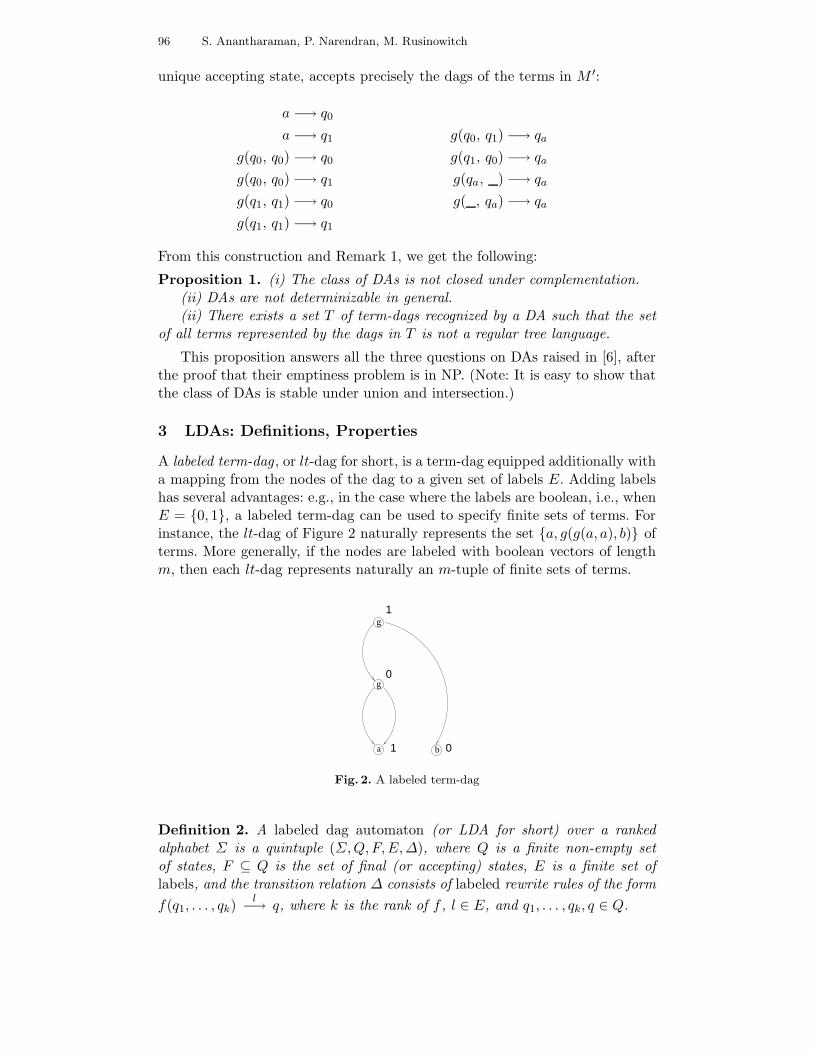
96 S. Anantharaman, P. Narendran, M. Rusinowitch
unique accepting state, accepts precisely the dags of the terms in M ′:
a −→ q0
a −→ q1
g(q0, q0) −→ q0
g(q0, q0) −→ q1
g(q1, q1) −→ q0
g(q1, q1) −→ q1
g(q0, q1) −→ qa
g(q1, q0) −→ qa
g(qa, ) −→ qa
g( , qa) −→ qa
From this construction and Remark 1, we get the following:
Proposition 1. (i) The class of DAs is not closed under complementation.(ii) DAs are not determinizable in general.(ii) There exists a set T of term-dags recognized by a DA such that the set
of all terms represented by the dags in T is not a regular tree language.
This proposition answers all the three questions on DAs raised in [6], afterthe proof that their emptiness problem is in NP. (Note: It is easy to show thatthe class of DAs is stable under union and intersection.)
3 LDAs: Definitions, Properties
A labeled term-dag , or lt-dag for short, is a term-dag equipped additionally witha mapping from the nodes of the dag to a given set of labels E. Adding labelshas several advantages: e.g., in the case where the labels are boolean, i.e., whenE = 0, 1, a labeled term-dag can be used to specify finite sets of terms. Forinstance, the lt-dag of Figure 2 naturally represents the set a, g(g(a, a), b) ofterms. More generally, if the nodes are labeled with boolean vectors of lengthm, then each lt-dag represents naturally an m-tuple of finite sets of terms.
g
g
a b
1
0
01
Fig. 2. A labeled term-dag
Definition 2. A labeled dag automaton (or LDA for short) over a rankedalphabet Σ is a quintuple (Σ,Q,F,E,∆), where Q is a finite non-empty setof states, F ⊆ Q is the set of final (or accepting) states, E is a finite set oflabels, and the transition relation ∆ consists of labeled rewrite rules of the form
f(q1, . . . , qk)l−→ q, where k is the rank of f , l ∈ E, and q1, . . . , qk, q ∈ Q.
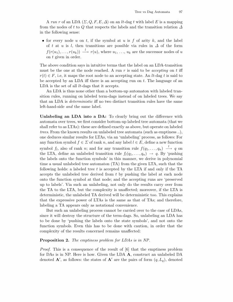
Tree vs Dag Automata 97
A run r of an LDA (Σ,Q,F,E,∆) on an lt-dag t with label E is a mappingfrom the nodes of t to Q that respects the labels and the transition relation ∆in the following sense:
• for every node u on t, if the symbol at u is f of arity k, and the labelof t at u is l, then transitions are possible via rules in ∆ of the form
f(r(u1), . . . , r(uk))l−→ r(u), where u1, . . ., uk are the successor nodes of u
on t given in order.
The above condition says in intuitive terms that the label on an LDA-transitionmust be the one at the node reached. A run r is said to be accepting on t iffr(t) ∈ F , i.e, it maps the root node to an accepting state. An lt-dag t is said tobe accepted by an LDA iff there is an accepting run on t. The language of anLDA is the set of all lt-dags that it accepts.
An LDA is thus none other than a bottom-up automaton with labeled tran-sition rules, running on labeled term-dags instead of on labeled trees. We saythat an LDA is deterministic iff no two distinct transition rules have the sameleft-hand-side and the same label.
Unlabeling an LDA into a DA: To clearly bring out the difference withautomata over trees, we first consider bottom-up labeled tree automata (that weshall refer to as LTAs): these are defined exactly as above, but operate on labeledtrees. From the known results on unlabeled tree automata (such as emptiness ..),one deduces similar results for LTAs, via an ‘unlabeling’ process, as follows: Forany function symbol f ∈ Σ of rank n, and any label l ∈ E, define a new function
symbol fl, also of rank n; and for any transition rule f(q1, . . . , qn)l−→ q on
the LTA, define an unlabeled transition rule fl(q1, . . . , qn) → q. By ‘pushingthe labels onto the function symbols’ in this manner, we derive in polynomialtime a usual unlabeled tree automaton (TA) from the given LTA, such that thefollowing holds: a labeled tree t is accepted by the LTA if and only if the TAaccepts the unlabeled tree derived from t by pushing the label at each nodeonto the function symbol at that node; and the accepting runs are ‘preservedup to labels’. Via such an unlabeling, not only do the results carry over fromthe TA to the LTA, but the complexity is unaffected; moreover, if the LTA isdeterministic, the unlabeled TA derived will be deterministic too. This explainsthat the expressive power of LTAs is the same as that of TAs; and therefore,labeling a TA appears only as notational convenience.
But such an unlabeling process cannot be carried over to the case of LDAs,since it will destroy the structure of the term-dags. So, unlabeling an LDA hasto be done by ‘pushing the labels onto the state symbols’, and not onto thefunction symbols. Even this has to be done with caution, in order that thecomplexity of the results concerned remains unaffected:
Proposition 2. The emptiness problem for LDAs is in NP.
Proof. This is a consequence of the result of [6] that the emptiness problemfor DAs is in NP. Here is how. Given the LDA A, construct an unlabeled DAdenoted A′, as follows: the states of A′ are the pairs of form (q, Lq), denoted

98 S. Anantharaman, P. Narendran, M. Rusinowitch
as q, where q is a state of A and Lq is the set of all labels of the transitionsof A which have q as target; the (unlabeled) transitions of A′ are of the form
f(q1, . . . , qk) −→ q, whenever f(q1, . . . , qk)l−→ q is a (labeled) transition on
the given LDA A; the accepting states of A′ are the q’s corresponding to theaccepting states q on A. Note that A′ is constructed from A in linear time: itsnumber of states is the same as for A (since Lq is completely determined by qon A), and its number of transitions is at most that of A.
It is not hard to check then that the LDA A has a non-empty language ifand only if the unlabeled DA A′ accepts some term-dag. ⊓⊔Remark 2. In the above construction of the unlabeled A′ from the LDA A,the accepting runs are preserved up to labels; but even if the LDA A is de-terministic, the DA A′ will be non-deterministic in general. This shows thatdeterministic LDAs do not behave in general like deterministic LTAs; it turnsout in particular, that their emptiness problem is NP-hard (so NP-complete,thanks to [6]):
Theorem 1. The emptiness problem is NP-hard for deterministic LDAs.
Proof. The proof is by reduction from boolean satisfiability. Let B be any arbi-trarily chosen boolean formula over a given set of boolean variables x1, . . . , xn,and the usual boolean connectives ∧,∨,¬. Let tB be a term-dag for B, and mits number of distinct nodes. We then construct an LDA A with 2m states, suchthat A accepts exactly the term-dag tB labeled suitably with boolean values0, 1 if and only if B is satisfiable. The construction goes as follows.
Corresponding to each node we have two states which stand for that sub-formula getting the corresponding truth-value. For ease of exposition we repre-sent the states in the form q(s,0) or q(s,1) where s is a subterm of tB . The labelsare 0 and 1. The labeled transition rules on A are of the form:
xi0−→ q(xi,0), xi
1−→ q(xi,1),
and, more generally, for any h ∈ ∧,∨, will have the form:
h(q(s1,b1), q(s2,b2))h(b1,b2)−−−−−→ q(h(s1,s2),h(b1,b2))
where b1, b2 ∈ 0, 1, and h(s1, s2) is a subterm of tB; for the connective ¬ we
have the transitions of the form: ¬(q(s,b))¬b−→ q(¬s,¬b). The unique accepting
state is q(tB ,1). This LDA meets the requirements (cf. [3]). ⊓⊔Remarks 3. i) By replacing the labels of the above constructed LDA by a“don’t-care” boolean label (the LDA becomes non-deterministic, but) we maydeduce that the membership problem for LDAs is NP-hard (so is NP-complete).
ii) The above proof is a further illustration that deterministic LDAs do notbehave like deterministic LTAs: the reason is that on a tree the same subtermcan be at two different nodes with different labels. Thus, a deterministic LTAcan be easily constructed to accept the boolean formula a ∧ ¬ a as a suitablylabeled tree.
iii) Exploiting the fact that on a dag two equal subterms must occupy thesame node, one can construct a DA that accepts precisely all the non-acceptingor incorrect computations of a deterministic 2-counter machine, cf. [3]. It followsthat the universality problem for DAs is undecidable, consequently so is alsothe problem of equivalence of DAs.

Tree vs Dag Automata 99
4 LDA for Solving a Unification Problem
This section presents briefly the ideas on how the LDA formalism was usedin [1], for solving the ACID-unification problem. (It was this problem thatwas the motivation for our initial interest in DAs and LDAs.) The full details –technical and complex – will be left out, but can be found in the research reportRR-2004-12: How useful are Dag Automata ?, http://www.univ-orleans.fr/lifo/prodsci/rapports/RR2004.htm.fr.
By ACID we mean the theory defined by the following equational axioms:
x+ (y + z) ≈ (x+ y) + z, x+ y ≈ y + x, x+ x ≈ x.
x ∗ (y + z) ≈ (x ∗ y) + (x ∗ z), (u+ v) ∗ w ≈ (u ∗ w) + (v ∗ w)
ACID-unification with free constants is the problem of solving, modulo thistheory, a finite family of equations of the form: s1 = t1, . . . , sk = tk as finite,non-empty sets of ground terms (over the free constants) for the variables ofthe problem. Such a problem can always be reduced to a standard form,: everyequation in the problem has one of the following forms (respectively referred toas of type ‘product’, ‘sum’, or ‘constant’ ):
x = y ∗ z, u = v +w, u = c
where u, v,w, x, y, z are variables and c is any constant or 0. Since ‘+’ is idem-potent and ‘∗’ distributes left and right over ‘+’, we may view this ACID-unification problem as a set constraint problem; e.g. if y and z are interpretedas sets of terms over ∗ and the constants, then y ∗ z = s ∗ t | s ∈ y, t ∈ z.
To every such problem P, we associate an LDA in such a way that solvingP amounts – in the following sense – to showing that the language of the LDAis non-empty. Let Xi, i = 1..n, denote the set variables of the problem P:
(i) If Si, i = 1..n, are (finite, non-empty) sets of ground terms such thatXi = Si, i = 1..n, is a solution to P, then one can construct an lt-dag repre-senting this family of sets (so labeled with boolean vectors of length n), suchthat the LDA associated accepts the lt-dag.
(ii) Conversely, if t is an lt-dag t (labeled with boolean vectors of length n)accepted by the LDA associated to P, the n sets of ground terms Si recoveredas elements of Xi from the labels of t may not have the closure property w.r.t.P, i.e. some of the ‘product’-equations of P may remain unsatisfied; however,from the accepting run of the LDA on t, we can derive a grammar, with thehelp of which one can produce a solution to the problem P.
Suppose given an ACID-unification problem P, and let Xii=1..n be its setvariables, arranged in some fixed order. The lt-dags on which we shall considerruns of our LDA (to be defined), will be term dags over the symbol ‘∗’ and thegiven ground constants, labeled with n-bit vectors at their various nodes. Theselabels will in general be denoted as (m1,m2, . . . ,mn), mi ∈ 0, 1, i = 1..n.They have as semantics that mi = 1 iff the subterm of the lt-dag at the currentnode is an element of the set Xi.
The LDA that we shall be associating with our ACID-problem is somewhatsimilar to the tree automata with free variables defined in [9]. Let S be the set ofall 2n-bit vectors of the form ..., li, ...; ..., hi , ... such that li ≤ hi for all i ∈ 1..n;the elements of S will be referred to as pstates; we denote them by barred capital

100 S. Anantharaman, P. Narendran, M. Rusinowitch
letters such as A,B, . . .. For any pstate A ∈ S, we shall be denoting its first-half(or lower) and second-half (or higher) n-bit vectors by A.l,A.h respectively.
Any state A of our LDA will have as its first component a pstate, that weshall denote A; this corresponds to two sets of boolean valuations on the setexpressions Xii=1..n ; the lower i-th bit A.li of the LDA state A will signify(when 1) that the term at the current node on an lt-dag mapped to A undera given run r is accepted as element of Xi; the upper i-th bit A.hi is meant tosignify (when 1) that some subterm below the current node has been acceptedin Xi by the run; this explains why we only consider pstates A with A.l ≤ A.h.
An accepting state on the LDA will then be in particular such that A.hi = 1for all i = 1..n; but this condition alone will not be sufficient for acceptance:many of the ‘product’-equations of P may still remain unsatisfied. To circum-vent this, we add as the second component of any state A of the LDA, a setof equalities formed from some new symbols called dsymbols which are meantto keep some book-keeping on the nodes traversed by the run. A dsymbol is ofthe form Xi
B, where 1 ≤ i ≤ n, and B is a pstate. The second component at
any state A will be referred as the defect set at A and denoted as MA; it willcontain some dsymbols doing the book-keeping along the run, together withsome defect equalities: a defect equality over the dsymbols is by definition anequality having one of the two following forms:
XkC
= XiAXj
B, T = Xi
AXj
B
where A,B,C ∈ S, and (k, i, j) are triples corresponding to some ‘product’-equation in P of the form Xk = Xi ∗ Xj . Equalities of the first type are saidto be closed, and those of the second type open. (Note: the number of all thedsymbols and defect equalities is polynomial in the size of S.)
The presence of a dsymbol XiB
in the defect set MA of a state A has thesemantics that some node below, along the run, got mapped to a state on theLDA whose pstate is B, and the subterm at that node is in the set Xi. Closed(resp. open) defect equalities in the defect set MA keep track of the ‘product’-equations of P which have remained ‘covered’ along the run (resp. which stillremain to be covered). The open defect equalities will also be witnesses that theterm accepted at the current node by the run contributes (along with a subtermaccepted at some earlier node) to one or more of the ‘product’-equations of P.
By definition, the accepting states of the LDA are the A satisfying the fol-lowing two conditions:
(i) A.hi = 1 for all i ∈ 1, .., n;(ii) the defect set MA at A contains no open defect equalities.
We skip the other technical details on how the transitions are defined on theLDA associated to P, in particular on how the pstates and the defect sets evolveunder them. Suffices to note that they are defined in such a way that the LDAwill be deterministic. (This fact is crucial for proving the completeness of theLDA approach for solving ACID-unification problems.)
We give below a couple of examples illustrating the approach sketched above;the first one shows in particular why we need a grammar from an accepted lt-dag to generate a solution for the unification problem. Guessing how the runsget initialized must not be too difficult, from either of the examples.

Tree vs Dag Automata 101
4.1 Examples of ACID-Unification
Example 1. Consider the ACID-problem Z =? X ∗ Y , and order the listof variables as X,Y,Z. Let a, b, c, d be ground constants; we construct anaccepted lt-dag rooted at (c ∗ (c ∗ (a ∗ b))) ∗ (c ∗ d), with leaves at a, c put intoX; and at b, d put into Y ; in addition the nodes at (a ∗ b), (c ∗ (a ∗ b)) are putinto Y ; cf. figure below. From the labels of this accepted lt-dag we only get thefollowing terms in the set Z: (a∗ b), c∗ (a∗ b), c∗ (c∗ (a∗ b)), (c∗d), so the setsof terms recovered from the labels of the lt-dag is not a solution to the problem.
The accepting run is as follows (in the figure, the states to which the nodesget mapped are indicated in italic capitals).
a, c100
−−−−−→ A = (100; 100; XA); b, d010
−−−−−→ B = (010; 010; YB);
A∗B011
−−−−−→ C = (011; 111; XA , YB , YC , ZC , ZC = XAYB, T = XAYC);
A ∗B001
−−−−−→ D = (001; 111; XA , YB , ZD, ZD = XAYB);
A∗C011
−−−−−→ C = (011; 111; XA , YB , YC , ZC , ZC = XAYB, T = XAYC);
C
c
a b
(a*b)
(c*(a*b))
(c*(c*(a*b)))
(c*(c*(a*b))) * (c*d)
d
(c*d)
(100) (010)
(010)
(011)(100)
(001)(011)
(001)
(000)
B
B
A
CA
D
F
G
Fig. 3. An accepted lt-dag for Z =? X ∗ Y
Then: A ∗ C001
−−−−−→ F = (001; 111;MF ), whereMF = XA, YB , YC , ZC , ZC = XAYB , ZF , ZF = XAYC.
And finally: F ∗D001
−−−−−→ G = (000; 111;MG), whereMG = XA, YB , YC , ZC , ZC = XAYB, ZD, ZD = XAYB, ZF , ZF = XAYC,
where D = F . The states D,F,G are all accepting; so the sub-dags rooted atthe nodes mapped to these states are accepted. The solution for the problemderived at the node mapped to D is the simplest; the assignment is: X =

102 S. Anantharaman, P. Narendran, M. Rusinowitch
A, Y = B, Z = A ∗B. where A −→ a | c, B −→ b | d; this is a correctsolution.
Let us compute the contribution of the run to X,Y,Z on the sub-dag rootedat node F , by looking at MF : The productions of the grammar w.r.t. thisaccepting sub-run are as follows:
F −→ A ∗ C, C −→ A ∗B, A −→ a | c, B −→ b | d.
So the contribution of the run is the assignment: X = A, Y = B, A ∗B, Z = A ∗B, A ∗ (A ∗B), where A −→ a | c, B −→ b | d; this is again acorrect solution.
The grammar for the accepting run at the root node G has an additionalproduction: D −→ A∗B, with D = F . The solution derived here is the same asat F : the terms derivable from this production are also derivable from C. ⊓⊔Example 2. The ACID-unification problem: X + Z = X ∗ Y + U may betransformed into the following standard form:
V = X + Z, V = W + U, W = X ∗ Y .
Let us show that the lt-dag in Figure 4 is accepted by the associated LDA.Arrange the set variables into an ordered list, say as X,Y,Z,U, V,W.
*
a
a*a (001011)
(110110)
Fig. 4. lt-dag solving V = X + Z, V = W + U, W = X ∗ Y
The states on the LDA are therefore 12-bit vectors. From the node ‘a’ onthe lt-dag with label m = (110110) we first have an initial transition to a stateA:
a110110−−−−−→ A = (110110 ; 110110 ;MA)
where MA = XA, YA, UA, VA, T = XAYA representing the fact that at thecurrent node the values X = Y = a = V = U have been accepted (anda product X ∗ Y remains to be covered). Next we have a transition, withlabel (001011), from A ∗ A to the state B = (001011; 111111;MB ), whereMB = XA, YA, UA, VA, ZB , VB ,WB ,WB = XAYA; at this node, the assign-ments W = a ∗ a = Z = V have been accepted. The state reached at the rootnode is an accepting state. So the lt-dag is accepted.
Note that in this case the lt-dag t has the closure property w.r.t. the problem:the sets of terms deduced from the labels of t is a solution to the ACID-problem.
On the other hand the grammar derived from the accepting run has twoproductions: B −→ A ∗ A, A −→ a. The contribution of the run to thevariables are therefore the sets of terms representable as: X = A = Y =U, V = A, A ∗ A, Z = W = A ∗A; that is to say:

Tree vs Dag Automata 103
X = a = Y = U, V = a, a ∗ a, Z = W = a ∗ awhich is the same as the one deduced from the labels of the lt-dag. ⊓⊔
5 Conclusion
The results of [3] that we have partially presented here illustrate that the alge-braic behavior of dag automata can be very different from that of tree automata.But at the same time the proof techniques employed in [3], as well as the ap-plication to unification that we have illustrated in Section 4, show that theexpressive power of dag automata can be extremely useful in modeling and/oranalyzing several complex situations. Furthermore, the dag representation hasbeen shown to be clearly space efficient for compressed XML documents, cf. [5,10, 11]. All these lead us to the belief that DAs and LDAs may also useful forhandling certain classes of XML/XPath queries, especially where bottom-upanalysis techniques can be brought into play.
References
1. S. Anantharaman, P. Narendran, M. Rusinowitch, ACID-Unification is NEXPTIME-Decidable, Proc. of MFCS’03, pp. 169–179, LNCS 2747, 2003.
2. S. Anantharaman, P. Narendran, M. Rusinowitch, Unification modulo ACUI plus Dis-tributivity Axioms, Journal of Automated Reasoning, Vol. 33, n01, pp.1–28, 2004.
3. S. Anantharaman, P. Narendran, M. Rusinowitch, Closure Properties and Decision Prob-lems of Dag Automata Information Processing Letters, (To appear), 2005.
4. F. Baader, P. Narendran, Unification of Concept Terms in Description Logics, Journal ofSymbolic Computation 31 (3):277–305, 2001.
5. P. Buneman, M. Grohe, C. Koch, Path queries on compressed XML. Proc. of the 29thConf. on VLDB, 2003, pp. 141–152, Ed. Morgan Kaufmann.
6. W. Charatonik, Automata on DAG Representations of Finite Trees, Technical ReportMPI-I-99-2-001, Max-Planck-Institut fur Informatik, Saarbrucken, Germany.
7. H. Comon, M. Dauchet, R. Gilleron, F. Jacquemard, D. Lugiez, S. Tison, M. Tommasi,Tree Automata Techniques and Applications, http://www.grappa.univ-lille3.fr/tata/
8. T. Genet and F. Klay, Rewriting for Cryptographic Protocol Verification, Proc. of the 17thCADE, pp. 271-290, LNAI 1831, 2000.
9. R. Gilleron, S. Tison, M. Tommasi, Set Constraints and Tree Automata, Information andComputation 149, 1–41, 1999. (cf. also Technical Report IT 292, Laboratoire-LIFL, Lille,1996.)
10. M. Frick, M. Grohe, C. Koch, Query Evaluation of Compressed Trees, Proc. of LICS’03,IEEE, pp. 188–197.
11. M. Marx. XPath and Modal Logics for Finite DAGs. Proc. of TABLEAUX’03, pp. 150–164, LNAI 2796, 2003.
12. M. Minsky, Computation: Finite and Infinite Machines, Prentice-Hall International,London, 1972.
13. F. Neven, Automata Theory for XML Researchers, SIGMO Record 31(3), September2002.
104 S. Anantharaman, P. Narendran, M. Rusinowitch
Relating Nominal and Higher-Order PatternUnification
James Cheney
University of [email protected]
Abstract. Higher-order pattern unification and nominal unification are twoapproaches to unifying modulo some form of α-equivalence (consistent renamingof bound names). The higher-order and nominal approaches seem superficiallydissimilar. However, we show that a natural concretion (or name-application)operation for nominal terms can be used to simulate the behavior of higher-order patterns. We describe a form of nominal terms called nominal patternsthat includes concretion and for which unification is equivalent to a special caseof higher-order pattern unification, and then show that full higher-order patternunification can be reduced to nominal unification via nominal patterns.
1 Introduction
Higher-order unification is the unification of simply-typed λ-terms up to α-, β-,and (sometimes) η-equivalence. It has been studied for over thirty years.. Al-though it is undecidable and of infinitary unification type, Huet’s algorithm [6]performs well in practice, and Miller identified a well-behaved special case calledhigher-order pattern unification [7, 13, 11, 1] that is decidable in linear timeand possesses unique most general unifiers. In higher-order patterns, uses ofmetavariables (variables for which terms may be substituted) are limited sothat the nondeterministic search needed in full higher-order unification can beavoided. A key aspect of higher-order unification is that substitution is capture-avoiding. For example, the unification problem λx.M ≈? λy.f y has no solution,since although both sides could be made equal by making a capturing substitu-tion f x for M , there is no way to make both sides equal using capture-avoidingsubstitution to instantiate M .
Nominal unification [15] is the unification of nominal terms, which includespecial name or atom symbols, a name-swapping operation, an abstraction op-eration for name-binding, and freshness relation. Equality and freshness fornominal terms coincide with classical definitions of α-equivalence and the “not-free-in” relation − 6∈ FV (−), respectively. Nominal unification is decidable inat worst quadratic time (exact complexity bounds are not yet known). Nomi-nal unification is based on nominal logic, a logic formalizing a novel approachto abstract syntax with bound names due to Gabbay and Pitts [3]. There aretwo aspects of nominal unification that contrast sharply with higher-order uni-fication. First, abstraction is not considered to bind names, and metavariablesmay mention arbitrary names, so that the problem 〈a〉M ≈? 〈b〉f(b) does havesolution M = f(a). Second, abstractions are not considered to be functions,and there is no built-in notion of “abstraction application”. Instead, nominalunifiers can be expressed in terms of the swapping operation (a b) · t, which
105

106 J. Cheney
describes the result of exchanging all occurrences of a and b within t, and fresh-ness constraints a # t, which assert that a name a is fresh for a term t. Forexample, the unification problem 〈a〉M ≈? 〈b〉f(N, b) has most general solutionM = f((a b) · N, a) subject to the constraint that a # N . This unifier showshow to compute M as a function of N while excluding false solutions such asM = f(b, a), N = a, since 〈a〉f(a, b) 6≈ 〈b〉f(b, a).
Despite these differences, nominal and higher-order pattern unification ap-pear closely related. In fact, at first glance, one might wonder if they are notmerely different presentations of the same algorithm. Both are techniques forequational reasoning about languages involving bound identifiers. Both algo-rithms rely on computing with permutations of bound names: the higher-order pattern restriction can be seen as a sufficient condition to ensure thatsuch permutations always exist. In fact, as noted by Urban, Pitts, and Gab-bay [15], there is a translation from nominal unification problems to higher-orderpattern unification problems that preserves satisfiability. In this translation,metavariables are “lifted” so as to be functions of all the names in context.A freshness constraint such as a # M can be translated to an equation likeλa, b, c.M a b c ≈ λa, b, c.N b c, which asserts that M cannot be dependenton its first argument (namely, a). However, as argued by Urban et al., it isnot straightforward to convert the resulting solutions back to solutions to theoriginal nominal unification problem. As a result, it appears much easier tosolve such problems directly using Urban et al.’s algorithm (which seems muchsimpler than that for higher-order pattern unification in any case).
Another reason to study the relationship between higher-order pattern uni-fication and nominal unification is to provide a logical foundation for higher-order patterns. While both nominal and higher-order unification are groundedin clear logical foundations, higher-order patterns appear motivated solely byalgorithmic concerns. If higher-order patterns can be explained using nominalterms, the semantic foundations of the latter could also be used for the former.
In this paper we argue that higher-order pattern unification can be reducedto nominal unification. This relationship helps justify the higher-order patternrestriction and explain why it works. The key idea is that the pattern restriction(that metavariable occurrences are of the form X v where v is a list of distinctnames) is essentially the same as a natural freshness restriction on the concretionoperation. This operation is an elimination form for abstraction that has beenconsidered in some versions of FreshML [12, 14], but so far not incorporatedinto nominal logic or nominal unification.
The structure of this paper is as follows. First (Section 2), we review higher-order pattern unification and nominal unification. In Section 3, we introducea type system that enforces the higher-order pattern restriction in a particu-larly convenient way. In Section 4, we identify a variant of nominal terms callednominal patterns that includes the concretion operation and for which unifica-tion is equivalent to a special case of higher-order pattern unification. We then(Section 5) show that full higher-order pattern unification can be reduced tonominal pattern unification and (Section 6) that nominal pattern unificationcan be reduced to nominal unification. Put together, these reductions show

Relating Nominal and Higher-Order Pattern Unification 107
that higher-order pattern unification can be implemented via nominal unifica-tion. Section 7 and Section 8 discuss related work and conclude.
2 Background
2.1 Higher-order terms, patterns, and unification
Consider infinite sets of variable names x, y, z, . . . ∈ Var and metavariablesX,Y,Z . . . ∈ MVar . The terms of the λ-calculus are as follows:
t ::= c | x | λx.t | t t′ | X
We assume that common notions such as the set of free variables of a termFV (−), α-equivalence, capture-avoiding substitution −[−/−] etc. are definedas usual. In addition, we assume that there are some given base types δ, thattypes include function types τ → τ ′, and that well-formedness is defined asusual provided that types are assigned to constants via a signature Σ. A termwith no free variables is called closed ; a term with no metavariables is calledground. We often write f(t1, . . . , tn) as a shorthand for f t1 · · · tn.
Terms are considered equal up to α-equivalence plus two additional equa-tions: β-reduction and η-expansion
(β) (λx.t) u ≈ t[u/x](η) t ≈ λx.(t x) (t : τ → τ ′, x 6∈ FV (t))
We write θ for a substitution mapping metavariables to λ-terms. Such asubstitution may be applied to any λ-term by replacing each metavariable Xwith θ(X). If Γ and Γ ′ are contexts consisting only of metavariables, we writesubstitution is well-formed (Γ ′ ⊢ θ : Γ ) provided that for each X : τ ∈ Γ ,Γ ′ ⊢ θ(X) : τ . Thus, there is no danger of variable capture during substitution,and we have:
Lemma 1. If Γ ⊢ θ : Γ ′ and Γ ′ ⊢ t : τ , then Γ ⊢ θ(t) : τ .
We consider higher-order unification to be unification of λ-terms up to theabove equational theory, that is, up to αβη-equivalence. (Higher-order unifica-tion sometimes refers to unification up to only α and β-equivalence, but forthis paper, we do not consider this problem.) Huet [6] gave an algorithm forgenerating complete sets of higher-order unifiers which performs well in prac-tice. Technically, we consider only problems of the form ∃X.∀y.t ≈? u, sincesubstitutions θ cannot mention free variables. This excludes problems such as∀y.∃X.X ≈? y. However, such problems can always be transformed to equiv-alent ∃∀-problems by raising [9] metavariables in order to make their depen-dence on other variables explicit: for example, transforming ∀y.∃X.X ≈? y to∃F.∀y.F y ≈? y, where X ≈ F y.
Miller investigated a decidable special case of higher-order unification calledhigher-order patterns. To define higher-order patterns, we first recall that anyλ-term (possibly involving metavariables) can be put into a normal form calledη-long, β-normal form (or ηlβn form), such that (a) no β-redices exist, and

108 J. Cheney
(b) no η-expansions can be performed without introducing a β-redex. Notethat this normal form is dependent on the types of metavariables. For example,the normal form of λy, z.(λx.xy) (F G) is λy, z, b.F (λa.G a) y b, providedF : (τ → τ ′) → σ1 → σ2 → σ and G : τ → τ ′. Such normal forms conform tothe following grammar:
t ::= λv.x t | λv.X t
The insight behind higher-order pattern unification is that all the nondetermin-ism in higher-order unification comes about because of uncertainty concerninghow an unknown X can act on its arguments t. In general, t may includerepeated variables or more complex terms involving other metavariables. Inhigher-order patterns, this uncertainty is eliminated by requiring the argumentlist t in each subterm of the form λv.X t to be a list of distinct bound variablesw. Thus, the above example ηlβn-normal form λy, z, b.F (λa.G a) y b is not apattern, while λx, y.c (F y x) is a pattern.
Higher-order patterns are closed under substitution modulo β-normalization;in fact, the only redices introduced by substituting a higher-order pattern for ametavariable in another higher-order pattern are of the form called β0 by Miller:
(β0) (λx.t) y = t[y/x]
Unification for higher-order patterns is decidable (in linear time [13]) and mostgeneral unifiers exist.
2.2 Nominal terms and unification
We now consider a different language called nominal terms1. Let ν, ν ′ be basicname types. Let Nm be a set of names aν , bν′ , . . . tagged with name types andlet MVar be a set of metavariables X,Y,Z, . . .. The set of nominal terms isgenerated by the grammar
t ::= aν | 〈aν〉t | c | t1 t2 | π ·X π ::= id | (aν bν) π
τ ::= σ | σ → τ σ ::= δ | ν | 〈ν〉δ
Metavariables are annotated with suspended permutations of names, that areto be applied to any value substituted for the variable. A nominal term withno metavariables is called ground.
Terms of the form 〈a〉t are called abstractions. An abstraction is an objectwith a single bound name. However, the name is not considered syntacticallybound as in a λ-abstraction; instead, an abstraction describes a semantic valuewith a bound name. For example, 〈a〉b and 〈b〉b are not considered to be the sameterm; however, they have the same meaning. In particular, while term equalitybehaves like (and is intended to model) α-equivalence for ground terms, this isnot the case for terms mentioning metavariables (e.g., the equation 〈a〉X ≈ 〈b〉Xis not valid in general).
1 Our version of nominal terms is superficially different from that used on Urban, Pitts,and Gabbay’s paper, in order to minimize the number of unimportant differences fromhigher-order patterns.

Relating Nominal and Higher-Order Pattern Unification 109
We assume that there is a signature Σ assigning types τ to constants c,such that there are no constants or other closed terms inhabiting any nametype. A permutation is considered well-formed if it is composed of swappingsof names of the same type only. Contexts Γ associate metavariables to types.The following well-formedness rules are considered:
Γ ⊢ aν : νc : τ ∈ ΣΓ ⊢ c : τ
π well-formedΓ,X : τ ⊢ π ·X : τ
Γ ⊢ t : τ → τ ′ Γ ⊢ u : τ ′
Γ ⊢ t u : τ ′Γ ⊢ t : τ
Γ ⊢ 〈aν〉t : 〈ν〉τ
We define a swapping function on nominal terms as follows:
(a b) · a′ =
b (a = a′)a (b = a′)a′ (a 6= a′ 6= b)
(a b) · c = c(a b) · (t1 t2) = ((a b) · t1) ((a b) · t2)
(a b) · 〈a〉t = 〈(a b) · a〉(a b) · t(a b) · (π ·X) = (a b) π ·X
Also, we define π · t as follows:
id · t = t (a b) (π · t) = ((a b) · π) · t
We are now in a position to define the meaning of nominal terms. We do thisby introducing axioms describing equality and an auxiliary freshness relation.
a ≈ a c ≈ ct ≈ t′ u ≈ u′
t u ≈ t′ u′t ≈ u
〈a〉t ≈ 〈a〉u
t ≈ (a b) · u a # u (a 6= b)
〈a〉t ≈ 〈b〉u
a 6= b
a # b a # c
a # t a # u
a # t u a # 〈a〉t
a # t (a 6= b)
a # 〈b〉t
Given a substitution function θ mapping metavariables to terms, we writeθ(t) for the result of applying substitution θ to term t. To be precise, thedefinition of substitution is as follows.
θ(a) = aθ(c) = c
θ(〈a〉t) = 〈a〉θ(t)θ(π ·X) = π · θ(X)
θ(t1 t2) = θ(t1) θ(t2)
We require that substitutions are well-formed so that they preserve types, but(unlike for higher-order unification) substitutions are allowed to mention bothmetavariables and names, so “capturing” substitutions are allowed. For exam-ple, if θ(X) = a then θ(〈a〉X) = 〈a〉a.
If θ is a valuation (ground substitution), we write θ t ≈ u to indicate thatθ(t) ≈ θ(u) and write θ a # t if a # θ(t). As usual, a formula A is valid(satisfiable) if for all (resp. some) well-formed substitutions, θ A holds. Thisis extended to validity or satisfiability of sets of formulas P in the obvious way.Similarly, if P is a set of formulas, we write P A to indicate that wheneverθ P , we also have θ A.
Urban et al.’s nominal unification algorithm solves the satisfiability problemfor sets of equations and freshness constraints. Given a problem P , it producesa unique (up to renaming) most general answer of the form θ,∇, where θ is

110 J. Cheney
a substitution and ∇ is a set of freshness constraints of the form a # X.This answer has the property that ∇ θ(P ). Moreover, for any other answer∇′, θ′ having this property, there exists a substitution ρ such that ρ(∇) ∇′
and ρ(∇) ρ θ ≈ θ′ (where θ ≈ θ′ means dom(θ) = dom(θ′) and ∀X ∈dom(θ).θ(X) ≈ θ′(X)).
Urban et al. argue that their algorithm can be implemented in quadratictime; however, the exact complexity has not been established. We omit theprecise details of the algorithm.
3 A Refined Type System for Higher-Order Patterns
We modify the notation of λ-terms to distinguish between rigid applications in-volving terms t u where the head of t is rigid (i.e., a constant or bound variable),and flexible applications tˆa, where the head of t is flexible (a metavariable).Also, we assume that variables are tagged with their types: for example, xτ in-dicates that x is a variable of type τ . The grammar of such terms is as follows:
t ::= c | xτ | λxτ .t | t t′ | X | tˆxτ
We use a type system for ηlβn-normalized terms that enforces the patternrestriction. Contexts Γ bind metavariables to types. There are three judgmentforms: Γ ⊢ t ↓ τ , indicating that t is a rigid atomic term of type τ ; Γ ⊢ t ⇓ τ ,indicating that t is a flexible atomic term of type τ ; and Γ ⊢ t ↑ τ , indicatingthat t is a normal term of type τ . Examples of rigid atomic, flexible atomic, andnormal terms include x (λy.y)z, X ˆyˆz, and λx, y, z.y (x (λy.y)z) (X ˆyˆz),respectively. The well-formedness rules for nominal patterns are as follows:
c : τ ∈ ΣΓ ⊢ c ↓ τ Γ ⊢ xτ ↓ τ
Γ ⊢ t ↑ τ ′
Γ ⊢ λxτ .t ↑ τ → τ ′Γ ⊢ t ↓ τ → τ ′ Γ ⊢ u ↑ τ
Γ ⊢ t u ↓ τ ′
Γ,X : τ ⊢ X ⇓ τ
Γ ⊢ t ⇓ τ → τ ′ (x 6∈ FV (t))
Γ ⊢ tˆxτ ⇓ τ′
Γ ⊢ t ↓ δ
Γ ⊢ t ↑ δ
Γ ⊢ t ⇓ δ
Γ ⊢ t ↑ δ
There is no way to bind a metavariable: λ binds ordinary variables only. Wecan only convert from an atomic typing to a normal typing at base types δ; thisensures that all the necessary η-expansions take place.
All well-formed terms in this system are ηlβn-normalized. Moreover, as forhigher-order patterns generally, only β0 reductions (λxτ .t)ˆyτ → t[yτ/xτ ] needto be performed after a substitution of higher-order patterns for metavariables.
Lemma 2 (Renaming). Let R be one of ↓,⇓, ↑. If yτ 6∈ FV (t) and Γ ⊢ t R τ ,then Γ ⊢ t[yτ/xτ ] R τ , respectively.
Lemma 3 (Substitution). If Γ,X : τ ′ ⊢ t ↑ τ and Γ ⊢ u ↑ τ ′ for FV (u) = ∅,then Γ ⊢ t[u/X] ↑ τ .
4 Nominal Patterns
We now introduce a slight variant of nominal terms that provides a closer matchto higher-order patterns. This language, called nominal patterns, is defined by

Relating Nominal and Higher-Order Pattern Unification 111
the following grammar:
t ::= c | t t′ | X | aν | 〈aν〉t | t@ aν
τ ::= σ | σ → τ σ ::= δ | ν | 〈ν〉σ
where as before, δ denotes a base (data) type and ν denotes a name type. Asbefore, we assume that there is a signature assigning τ -types to constants c.Metavariables may not have arbitrary types, but only σ-types (i.e., types builtusing only data, name, and abstraction types). In addition, we assume thatname symbols aν are tagged with their name types ν. As for nominal terms, weassume that the only ground terms inhabiting name-types are literal names.
The main difference between ordinary nominal terms and nominal patternsis the presence of the concretion operation (−)@(−) that has also been consid-ered in some versions of FreshML [12, 14]. Our type system requires well-formednominal patterns to satisfy an analogue of the higher-order pattern restriction:in every subterm of the form t@a, we require that a # t holds. In order tosimplify this check (and to make nominal patterns more similar to higher-orderpatterns), we only consider substitutions of patterns such that FN(t) = ∅,where
FN(c) = ∅ FN(X) = ∅
FN(a) = a FN(t u) = FN(t) ∪ FN(u)FN(t@a) = FN(t) ∪ a FN(〈a〉t) = FN(t)− a
As a result, a # X and (a b) · X ≈ X are valid for any names a, b andmetavariable X; using these facts we can lift the freshness relation and swappingfunction to patterns involving metavariables.
As before, signatures Σ map constants to types and names to name types,whereas contexts map metavariables to metavariable types σ. We require pat-terns to be well-typed, subject to the following rules:
Γ ⊢ aν ↓ νc : τ ∈ ΣΓ ⊢ c ↓ τ Γ,X : σ ⊢ X ↓ σ
Γ ⊢ t ↓ τ → τ ′ Γ ⊢ u ↑ τ
Γ ⊢ t u ↓ τ ′
Γ ⊢ t ↑ σ
Γ ⊢ 〈aν〉t ↑ 〈ν〉σ
Γ ⊢ t ↓ 〈ν〉σ a 6∈ FN(t)
Γ ⊢ t@aν ↓ σ
Γ ⊢ t ↓ ǫ (ǫ = δ, ν)
Γ ⊢ t ↑ ǫ
Abstraction and concretion are construction and destruction operations for theabstraction sort. Thus, nominal patterns are subject to the following βα- andηα-laws:
(βα) (〈a〉t)@b ≈ (a b) · t(ηα) t ≈ 〈a〉(t@a) (t : 〈ν〉σ)
Note that the typing rules ensure that b # 〈a〉t must hold in the first case anda # t must hold in the second case. We first state some basic properties ofnominal patterns.
Lemma 4 (Swapping). Let R be one of ↓, ↑. If Γ ⊢ t R τ then Γ ⊢ (a b)·t R τ .
Lemma 5 (Substitution). If Γ,X : τ ′ ⊢ t ↑ τ and Γ ⊢ u ↑ τ ′ where FN(u) =∅, then Γ ⊢ t[u/X] ↑ τ .

112 J. Cheney
We now show that this axiomatization satisfies the previously given laws ofnominal abstraction.
Proposition 1. For nominal patterns, we have 〈a〉t ≈ 〈b〉u if and only if a ≈b, t ≈ u or a # u, t ≈ (a b) · u. Similarly, if t : 〈ν〉τ , then there exists aν andu : τ such that t ≈ 〈a〉u.
Proof. Suppose 〈a〉t ≈ 〈b〉u. Then a # 〈a〉t ≈ 〈b〉u, so we have
t ≈ (a a) · t ≈ (〈a〉t)@a ≈ (〈b〉u)@a ≈ (a b) · u
There are two cases. If a = b then t ≈ (a b) ·u = (a a) ·u = u. Otherwise, a # uand t ≈ (a b) · u.
Now suppose t : 〈ν〉τ . Since FN(t) is finite, we can always find a name a 6∈FN(t), so we can form the term 〈a〉(t@a). By the η-rule, we have t ≈ 〈a〉(t@a),thus, a is the required name and t@a the required term of type τ .
The similarity between the βα and ηα rules for nominal patterns and theβ0 and η rules for higher-order patterns is not a coincidence. We now considera typed translation from nominal to higher-order patterns. We assume (forconvenience) that the constants, names and metavariables of nominal patternsare the same as the constants, variables, and metavariables of higher-orderpatterns respectively. Similarly, we assume that the name types and data typesof the nominal language are base types of the higher-order language. Terms aretranslated as follows:
c∗ = c(t u)∗ = t∗ u∗
X∗ = X
a∗ν = aν
(〈aν〉t)∗ = λaν .t
∗
(t@aν)∗ = (t∗)ˆaν
The translation of types is as follows:
δ∗ = δν∗ = ν
(σ → τ)∗ = σ∗ → τ∗
(〈ν〉τ)∗ = ν → τ∗
Contexts and signatures are translated by replacing each type with its starredform.
Example 1. The translation of t = 〈a〉X @ a@ b is λa.X a b, where X : 〈ν〉〈ν〉δin the former and X : ν → ν → δ in the latter.
Lemma 6. If a 6∈ FN(t) then a∗ 6∈ FV (t∗). Also, if Γ ⊢ t ↑ τ then Γ ∗ ⊢ t∗ ↑τ∗.
Theorem 1. The translation (−)∗ has an inverse (−)† on its range.
Proof. Clearly (−)∗ is injective, and it is surjective on its range by definition.
Lemma 7. If Γ ⊢ t : τ is a nominal pattern and b 6∈ FN(t), then ((a b) · t)∗ =t∗[b/a]. Dually, if Γ ⊢ u : τ is a higher-order pattern in the range of (−)∗, andb 6∈ FV (t), then (u[a/b])† = (a b) · u†.

Relating Nominal and Higher-Order Pattern Unification 113
Proof. Proof is by induction on the structure of t. If t = a, then ((a b) · t)∗ =b∗ = b and t∗[b/a] = a[b/a] = b. Otherwise, t is a name other than a or b,and swapping, substitution, and the (−)∗ translation all fix t. The case fort a constant or metavariable is similar. For t = t1 t2, the induction step isstraightforward. This leaves the case of abstraction. If t = 〈a〉u, then b # u soby induction we have ((a b) · u)∗ = u∗[b/a], hence
((a b) · 〈a〉u)∗ = (〈b〉(a b) · u)∗ = λb.((a b) · u)∗ = λb.u∗[b/a]
≈α λa.u∗ = (λa.u∗)[b/a] = (〈a〉u)∗[b/a]
If t = 〈b〉u, then the induction hypothesis does not apply directly, but we canchoose a fresh name b′ # a, b, t such that
((a b) · 〈b〉t)∗ ≈ ((a b) · 〈b′〉(b b′) · t)∗ = (〈b′〉(a b) · (b b′) · t)∗
= λb′.((b b′) · t)∗[b/a] = λb′.t∗[b′/b][b/a] ≈α λb.t∗[b/a] = (〈b〉t)∗[b/a]
where the two middle steps rely on the facts that b 6∈ FN((b b′) · t) and b′ 6∈FN(t). The case for t = 〈a′〉t for a′ 6= a, b is straightforward.
The second part follows immediately from the first by setting t = u†.
Theorem 2. Let t, u : τ be nominal patterns. Then t ≈ u if and only if t∗ ≈ u∗.
Proof. Proof is by induction on the derivation of t ≈ u in the forward direction.The interesting cases are for βα and ηα rules. While ηα is straightforward, forβα we have (〈a〉t)@b ≈ (a b) · t and want to show that (λa.t∗) b ≈ ((a b) · t)∗.By β0 and the previous lemma we have (λa.t∗) b ≈ t∗[b/a] = ((a b) · t)∗.
The reverse direction is similar, except that we need to use the identity(t[a/b])† = (a b) · t† in the β0 case.
Corollary 1. t ≈ u is satisfiable if and only if t∗ ≈ u∗ is; moreover, the satis-fying valuations θ, θ∗ are in bijective correspondence via (−)∗.
This shows that nominal pattern unification coincides with a special caseof higher-order pattern unification: specifically, the case for terms in which theonly form of binding is λ-abstraction over void base types ν. In fact, many ap-plications of higher-order patterns are possible within this fragment: it is com-monplace to use an abstract or empty type for the “type of variable names”in, for example, a higher-order abstract syntax encoding of the π-calculus [10].However, applications involving λ-abstraction over non-void types are also com-mon [7].
This translation is interesting, but we have only shown that there is a corre-spondence between two very limited special cases of the two problems. Next weshow how to translate full higher-order pattern unification to nominal patternunification.
5 Higher-order pattern unification as nominal patternunification
In higher-order patterns, λ-term variables are not limited to a collection of voidbase types, but may be of any type, so variables may be applied to argument

114 J. Cheney
lists including repeated variables, metavariables, or more general terms (thatis, the pattern restriction is not required of argument lists whose head is nota variable). This permits the formation of terms such as λx, y.y (λz.Fz) x xwhich are not in the range of (−)∗; i.e., which do not correspond to a nominalpattern. Such terms are not in the domain of (−)†, so the approach investigatedin the last section does not apply.
However, there is another translation that works. The reason the idea of theprevious section doesn’t work is that in higher-order patterns, variables playone of two roles: they can be passed as arguments to metavariables, but theycan also act as functions on lists of arguments. The latter role is not supporteddirectly by nominal patterns, because name types ν are populated only bynames.
Given a higher-order language L, we construct a nominal language L∗∗ pos-sessing a name-type ντ for each simple type τ of L and a data type δ for eachbasic type δ of L. We define a translation on L-types as follows:
δ∗∗ = δ (τ1 → τ2)∗∗ = 〈ντ1〉τ2
∗∗
Note that each τ -type of L translates to a σ-type of L∗∗. Given a signatureΣ, we write Σ∗∗ for the result of replacing all the types in Σ with their (−)∗∗
translations; similarly for contexts Γ ∗∗. Moreover, we add the following newconstants to L∗∗:
varτ : ντ → τ∗∗
appτ1τ2 : (τ1 → τ2)∗∗ → τ1
∗∗ → τ2∗∗
This signature is infinite, since the function symbols varτ and appτ1τ2 are in-dexed with types. However, in any particular situation, only finitely many ντ
types and finitely many constants of the above signature need to be considered.After unwinding definitions, the type of appτ1τ2 is 〈ντ1〉τ2
∗∗ → τ1∗∗ → τ2
∗∗. Thetypes of these constants are legal τ -types in L∗∗.
Intuitively, ντ is the type of names of variables of type τ , and var “casts”a ντ to its value, simulating the evaluation of a variable at the head of anapplication in a higher-order term. Similarly, app simulates application: givenan abstraction 〈ντ1〉τ2
∗∗ and a translated term of type τ1∗∗, application produces
a term of type τ2∗∗.
The idea of the translation is to use the var, app, and lam constructors torepresent ground λ-term structure, and use names, abstraction and concretionto represent subterms involving metavariables. In this translation, we assumethat λ-calculus variables are the same kinds of symbols as names in nominalpatterns.
c∗∗ = cxτ
∗∗ = var(xντ )(λx.t)∗∗ = 〈x〉t∗∗
(t u)∗∗ = app(t∗∗, u∗∗)X∗∗ = X
(tˆa)∗∗ = t∗∗ @ a
Example 2. Note that variable occurrences are treated differently dependingon context: variables on the left-hand side of a flexible application (−) (−) areleft alone, while others are encapsulated in a var(−)-constructor which casts a

Relating Nominal and Higher-Order Pattern Unification 115
variable name of type ντ to an expression of type τ∗∗. Thus, the translation ofλx, y.c (F ˆxˆy) is 〈x〉〈y〉app(var(c), F @x@ y), where F : τ1 → τ2 → δ in theformer is mapped to F : 〈ντ1〉〈ντ2〉δ in the latter.
The translation preserves well-formedness and is invertible; these facts areeasy to show by induction.
Proposition 2. If x 6∈ FV (t) then x∗∗ 6∈ FN(t∗∗). If Γ ⊢ t ↑ τ where t is ahigher-order pattern, then Γ ∗∗ ⊢ t∗∗ ↑ τ∗∗. Similarly, if Γ ⊢ t ↓ τ or Γ ⊢ t ⇓ τ ,then Γ ∗∗ ⊢ t∗∗ ↓ τ∗∗. Also, the translation has an inverse (−)††.
As observed by Miller, in a ηlβn higher-order pattern unification problem,the only kinds of redices that occur are β0 redices. Since the β0η theory is simu-lated by the βαηα theory in nominal patterns, higher-order pattern unificationis equivalent to nominal pattern unification.
Theorem 3. A higher-order pattern unification problem t ≈? u in ηlβn-normalform has a solution if and only if its translation t∗∗ ≈? u∗∗ has a nominal patternunifier.
Proof. For the forward direction, suppose that t, u are normalized and have ahigher-order pattern unifier θ, so that θ(t) ≈ θ(u) up to ηlβn-normalization.Moreover, this normalization process can only involve β0-redices, because thereare no metavariables of extensional function types in t, u (as argued above). Letθ∗∗ = [X := θ(X)∗∗ | X ∈ Dom(θ)] be the translation of θ. Following a similarargument to the one used in Theorem 2, β0-normalization can be simulatedin the nominal pattern calculus via βα-normalization. Thus, θ∗∗ is a nominalpattern unifier of t∗∗ ≈? u∗∗.
The reverse direction is similar. Since only βα-redices can be introduced ina nominal pattern unifier θ for t∗∗ ≈? u∗∗, we can use the reverse translation(−)†† to translate θ to a higher-order pattern unifier 膆.
6 Nominal Pattern Unification as Nominal Unification
In this section, we show how to reduce nominal pattern unification to nominalunification. This is not as trivial as it sounds, for nominal patterns includethe concretion operation not found in ordinary nominal terms, and so nominalpattern unification is not an immediate special case of nominal unification.In addition, nominal unification permits metavariables to be instantiated withterms containing free names, whereas nominal pattern unifiers must be closed.
We deal with the second problem first. Given a problem P with metavari-ables X and names a, let #(a,X) = a # X | a ∈ a,X ∈ X. This set ofconstraints ensures that no name mentioned in P can appear free in any substi-tution for P ’s metavariables. Moreover, the nominal unifiers produced by Urbanet al.’s algorithm only involve the names mentioned in the original problem.
Concretion can be eliminated from nominal pattern unification problems asfollows. If t@ a is a subterm of a nominal pattern unification problem P [t@ a],then that problem is equivalent to the problem P [Y ], 〈a〉Y ≈? t, where Y is afresh metavariable. This is because we know that a must be fresh for t (because
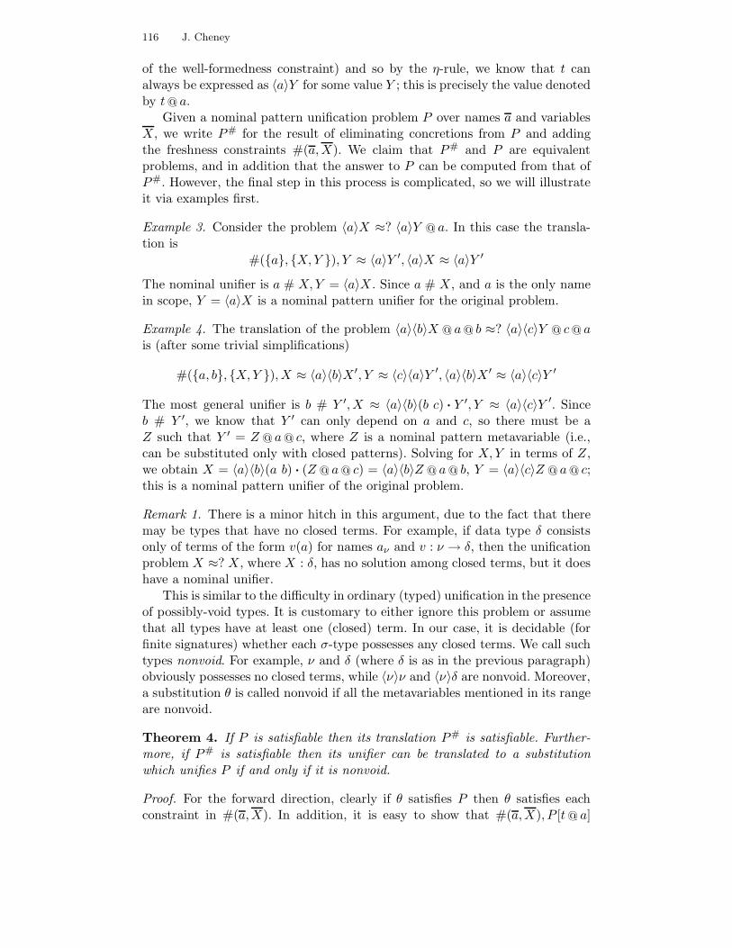
116 J. Cheney
of the well-formedness constraint) and so by the η-rule, we know that t canalways be expressed as 〈a〉Y for some value Y ; this is precisely the value denotedby t@ a.
Given a nominal pattern unification problem P over names a and variablesX, we write P# for the result of eliminating concretions from P and addingthe freshness constraints #(a,X). We claim that P# and P are equivalentproblems, and in addition that the answer to P can be computed from that ofP#. However, the final step in this process is complicated, so we will illustrateit via examples first.
Example 3. Consider the problem 〈a〉X ≈? 〈a〉Y @ a. In this case the transla-tion is
#(a, X,Y ), Y ≈ 〈a〉Y ′, 〈a〉X ≈ 〈a〉Y ′
The nominal unifier is a # X,Y = 〈a〉X . Since a # X, and a is the only namein scope, Y = 〈a〉X is a nominal pattern unifier for the original problem.
Example 4. The translation of the problem 〈a〉〈b〉X @ a@ b ≈? 〈a〉〈c〉Y @ c@ ais (after some trivial simplifications)
#(a, b, X,Y ),X ≈ 〈a〉〈b〉X ′, Y ≈ 〈c〉〈a〉Y ′, 〈a〉〈b〉X ′ ≈ 〈a〉〈c〉Y ′
The most general unifier is b # Y ′,X ≈ 〈a〉〈b〉(b c) · Y ′, Y ≈ 〈a〉〈c〉Y ′. Sinceb # Y ′, we know that Y ′ can only depend on a and c, so there must be aZ such that Y ′ = Z @ a@ c, where Z is a nominal pattern metavariable (i.e.,can be substituted only with closed patterns). Solving for X,Y in terms of Z,we obtain X = 〈a〉〈b〉(a b) · (Z @ a@ c) = 〈a〉〈b〉Z @ a@ b, Y = 〈a〉〈c〉Z @ a@ c;this is a nominal pattern unifier of the original problem.
Remark 1. There is a minor hitch in this argument, due to the fact that theremay be types that have no closed terms. For example, if data type δ consistsonly of terms of the form v(a) for names aν and v : ν → δ, then the unificationproblem X ≈? X, where X : δ, has no solution among closed terms, but it doeshave a nominal unifier.
This is similar to the difficulty in ordinary (typed) unification in the presenceof possibly-void types. It is customary to either ignore this problem or assumethat all types have at least one (closed) term. In our case, it is decidable (forfinite signatures) whether each σ-type possesses any closed terms. We call suchtypes nonvoid. For example, ν and δ (where δ is as in the previous paragraph)obviously possesses no closed terms, while 〈ν〉ν and 〈ν〉δ are nonvoid. Moreover,a substitution θ is called nonvoid if all the metavariables mentioned in its rangeare nonvoid.
Theorem 4. If P is satisfiable then its translation P# is satisfiable. Further-more, if P# is satisfiable then its unifier can be translated to a substitutionwhich unifies P if and only if it is nonvoid.
Proof. For the forward direction, clearly if θ satisfies P then θ satisfies eachconstraint in #(a,X). In addition, it is easy to show that #(a,X), P [t@ a]

Relating Nominal and Higher-Order Pattern Unification 117
is satisfiable if and only if #(a,X), P [Y ], 〈a〉Y ≈? t is satisfiable; thus, byinduction if P is satisfiable then so is P#.
For the reverse direction, suppose ∇, θ is the most general nominal unifierfor P#. Let a be the names of P . Suppose that the free variables in ∇, θ areY . For each Y ∈ Y , there is a list of names aYi
such that a ∈ A but a #Yi 6∈ ∇. Thus, we have Yi = Zi @ aYi
for some fresh metavariables Zi suchthat a # Zi. If we make this substitution, then we obtain a nominal patternpossibly involving swappings, but these swappings can be eliminated since eachZi satisfies (ai aj) · Z ≈ Z. This produces the desired substitution θ′. If θ′ isnonvoid, i.e. each σi is nonvoid for Zi : σi, then each Zi can be replaced witha closed term 0σi
to obtain a satisfying valuation for P . Conversely, it is notdifficult to show that if θ′ is not nonvoid, then P is unsatisfiable, since (bythe first part) any valuation satisfying P can be used to construct a valuationsatisfying P#, which would have to be an instance of ∇, θ because it is mostgeneral. Closed instantiations of all the Zi could be extracted from such avaluation.
7 Related work
As discussed by Urban et al. [15], nominal unification can apparently be reducedto higher-order pattern unification, but it is difficult to see how to translate theresulting higher-order pattern unifier to a nominal unifier. Nevertheless, sucha translation is of interest because if nominal unifiers can be extracted fromhigher-order pattern unifiers in linear time, this would give a linear algorithmfor nominal unification. We believe that it would be equivalent (and notationallysimpler) to investigate the reduction of full nominal unification to nominalpattern unification.
Miller [8] showed that higher-order unification problems (and higher-orderlogic programs) can be translated to logic programs in Lλ [7], a logic program-ming language based on higher-order pattern unification. This reduction takesadvantage of hereditary Harrop goals and clauses featured in Lλ. We believethat a similar reduction could be performed in a nominal logic programminglanguage that provides hereditary Harrop goals and program clauses. Whilesuch features are present in the current implementation of the nominal logicprogramming language αProlog, the semantics of goals of the form ∀x.G andD ⊃ G have not been studied carefully yet for nominal logic programming.This question, and more generally, the question of whether Lλ programs can betranslated to nominal logic programs (or vice versa) is of interest.
Hamana [4] has investigated the problem of unification modulo the β0-rulefor binding algebra terms [2]. Such terms are similar to nominal or higher-orderpatterns except that the lists of names supplied to metavariables may includerepeated names. As a result, unification appears to require some searching forsuitable renamings, and most general unifiers appear not to be unique. Obvi-ously, this is a special case of higher-order unification, but it appears to be atworst of nondeterministic polynomial time complexity (since one can guess asequence of appropriate renamings to find a unifier in polynomial time). We are

118 J. Cheney
interested in seeing whether this form of unification can also be implementedvia nominal logic programming using Miller’s approach.
Finally, we are interested in combining nominal and higher-order unification,or more generally, developing nominal equational unification techniques that in-clude higher-order unification, Hamana’s β0-unification, structural equivalencein the π-calculus, and other equational theories involving name-binding as spe-cial cases. We believe that nominal equational unification techniques would beextremely useful for programming, prototyping, and formalizing programminglanguages, logics, and type systems.
8 Conclusion
We have shown that higher-order pattern unification can be reduced to nominalunification via an intermediate language of nominal patterns. This shows thatany computation that can be performed using higher-order pattern unificationcan also be performed using nominal unification. It also shows that higher-orderpatterns are not just an ad-hoc invention of interest for efficiency reasons, butthat they can be given formal status using nominal logic: in particular, semanticmodels of binding syntax for higher-order patterns can be constructed using thesame techniques as for nominal logic.
Previous work has been focused on determining whether nominal unificationis really “new” (that is, whether it is trivially reducible to higher-order patternmatching). We agree with Urban et al. that while it may not be new, thereare good reasons for studying nominal unification directly rather than throughthe lens of higher-order unification. Moreover, our experience has been thatnominal unification is much closer to first-order unification and considerablysimpler to explain and implement than higher-order pattern unification (com-pare Urban et al. [15] to treatments such as Miller [7, 8], Nipkow [11], Doweket al. [1], or Hamana [5]). This is not meant as a criticism of these works! In-stead, our point is that even if one does not believe that nominal techniquesare worth investigating as an alternative to higher-order abstract syntax, webelieve that they are of value as an aid to understanding higher-order abstractsyntax, particularly higher-order patterns.
References
1. G. Dowek, T. Hardin, C. Kirchner, and F. Pfenning. Unification via explicit substitutions:The case of higher-order patterns. Technical Report Rapport de Recherche 3591, INRIA,December 1998.
2. M. P. Fiore, G. D. Plotkin, and D. Turi. Abstract syntax and variable binding. InGiuseppe Longo, editor, Proceedings of the 14th Annual IEEE Symposium on Logic inComputer Science, pages 193–202, Washington, DC, 1999. IEEE, IEEE Press.
3. M. J. Gabbay and A. M. Pitts. A new approach to abstract syntax with variable binding.Formal Aspects of Computing, 13:341–363, 2002.
4. Makoto Hamana. A logic programming language based on binding algebras. In Proc.Theoretical Aspects of Computer Science (TACS 2001), number 2215 in Lecture Notes inComputer Science, pages 243–262. Springer-Verlag, 2001.
5. Makoto Hamana. Simple β0-unification for terms with context holes. In Proceedings ofthe 16th International Workshop on Unification (UNIF 2002), pages 9–13, 2002.

Relating Nominal and Higher-Order Pattern Unification 119
6. Gerard Huet. A unification algorithm for typed λ-calculus. Theoretical Computer Science,1:27–67, 1975.
7. Dale Miller. A logic programming language with lambda-abstraction, function variables,and simple unification. J. Logic and Computation, 1(4):497–536, 1991.
8. Dale Miller. Unification of simply typed lambda-terms as logic programming. In KoichiFurukawa, editor, Logic Programming, Proceedings of the Eighth International Conference,pages 255–269, Paris, France, June 24–28 1991. MIT Press.
9. Dale Miller. Unification under a mixed prefix. Journal of Symbolic Computation,14(4):321–358, 1992.
10. Dale Miller and Alwen Tiu. A proof theory for generic judgments: extended abstract.In Proc. 18th Symp. on Logic in Computer Science (LICS 2003), pages 118–127. IEEEPress, 2003.
11. Tobias Nipkow. Functional unification of higher-order patterns. In Proc. 8th IEEE Symp.Logic in Computer Science, pages 64–74, 1993.
12. A. M. Pitts and M. J. Gabbay. A metalanguage for programming with bound namesmodulo renaming. In R. Backhouse and J. N. Oliveira, editors, Proc. 5th Int. Conf. onMathematics of Programme Construction (MPC2000), number 1837 in Lecture Notes inComputer Science, pages 230–255, Ponte de Lima, Portugal, July 2000. Springer-Verlag.
13. Zhenyu Qian. Linear unification of higher-order patterns. In Proceedings of the Interna-tional Joint Conference CAAP/FASE on Theory and Practice of Software Development,pages 391–405. Springer-Verlag, 1993.
14. M. R. Shinwell, A. M. Pitts, and M. J. Gabbay. FreshML: Programmming with bindersmade simple. In Proc. 8th ACM SIGPLAN Int. Conf. on Functional Programming (ICFP2003), pages 263–274, Uppsala, Sweden, 2003. ACM Press.
15. C. Urban, A. M. Pitts, and M. J. Gabbay. Nominal unification. Theoretical ComputerScience, 323(1–3):473–497, 2004.

120 J. Cheney
Efficiently Computable Classes of Second OrderPredicate Schema Matching Problems
Masateru HARAO1, Shuping YIN2, Keizo YAMADA1, and Kouichi HIRATA1
1 Department of Artificial Intelligence Kyushu Institute of TechnologyKawazu 680-4, Iizuka 820-8502, Japan
2 Graduate School of Computer Science and Systems Engineeringharao,yin,yamada,[email protected] ⋆
Abstract. Second order predicate schema matching is concerned with findingthe matchers of a given pair such that 〈Φ, φ〉 where Φ is a formula containingsecond-order predicate variables and φ is a first order logical formula. In general,this problem is intractable even if we impose some strict syntactic restrictions.In this paper, we propose a class of second order predicate schemas which isdefined by introducing syntax free variables and show that the computationalcomplexity of the schema matching is almost linear on input size. We also showthat this class possesses enough expressive power to implement a schema-guidedautomatic theorem prover.
1 Introduction
A schema is a template of formulas and knowledge processing which usesschemas as guiding information is called schema guided knowledge processing [6].Especially, processing based on second-order schemas has been studied in re-search areas such that program transformations [12], automatic program syn-theses [6], analogical reasoning [2, 4, 7], and so on. Here, second order matchinghas an important role in implementing these systems.
A second order predicate schema is a formula including second-order pred-icate variables, and a second order predicate schema matching is a problemof obtaining matchers of any pair such that 〈Φ, φ〉 where Φ is a second orderpredicate schema and φ is a closed first order formula. This predicate schemamatching can be regarded as a special case of the second-order matching andis known to be intractable in general [16].
Though the second-order matching is intractable in general [1], a sharp char-acterization between tractable and intractable second-order matching has beengiven from syntactical viewpoint [10]. Especially, a class of second order termscalled higher order pattern in which matchers can be derived in linear time hasbeen reported [14]. Furthermore, it has been shown that a matching algorithmwhich works more efficient than the standard one [11, 12] can be designed by us-ing pre-checking method [3]. These results indicate that the efficiency of secondorder matchings strongly depends on the existence of bound and free variablesand can be improved by devising the strategy of the procedure.
⋆ This work is partially supported by Grand-in-Aid for Scientific Research 13558036 from theMinistry of Education, Culture, Sports, Science and Technology, Japan, and Foundationfor promotion of researches on artificial intelligence
121

122 M. Harao, S. Yin, K. Yamada, K. Hirata
In this paper, we propose a class of second order predicate schemas inwhich an efficient schema matching exists from the motivation of construct-ing a schema-guided theorem prover [17]. Firstly, we define the syntax of sec-ond order schemas which we propose here by introducing syntax free variables.Next, we design a general schema matching algorithm based on the projectionposition indexing. Furthermore, we study the heuristics to improve its computa-tional efficiency. In particular, we present an algorithm which derives matchersefficiently by introducing strategy. Finally, we introduce a class of predicateschema matching problems in which a unique matcher can be derived almostin linear time. We also show that this class possesses enough expressive powerto implement a schema-guided automatic theorem prover.
2 Preliminaries
We use a term language L to represent second order language [10] instead of thegeneral language defined by using λ-notation. The term language L is definedusing the following symbol sets.
(1) IC :a set of individual constants a, b, c, . . .(2) IV :a set of individual variables x, y, z, . . .,(3) FC :a set of function constants f, g, h, . . .,(4) FV :a set of function variables F,G,H, . . .,(5) PC :a set of predicate constants p, q, r, . . .,(6) PV :a set of predicate variables P,Q,R, . . .,(7) ISV : a set of individual syntax variables xc, yc, zc, . . .,(8) FSV : a set of function syntax variables Fc, Gc,Hc, . . .,
Throughout of this paper, we assume a set of elementary types containingthe Boolean type o. Furthermore, we assume that each d ∈ IC ∪ IV ∪ FC ∪PC ∪ PV ∪ ISV ∪ FSV has a type denoted by τ(d). Each d ∈ IC ∪ IV ∪ ISVhas an elementary type not equal to o, each d ∈ FC ∪ FV ∪ FSV has a typeµ1 × · · · × µn → µ where neither µi nor µ is o, and each d ∈ PC ∪ PV has atype µ1 × · · · × µn → o. Especially, we deal with the logical connectives ∧,∨,⊃as predicate constants satisfying that τ(∧) = τ(∨) = τ(⊃) = o × o → o andτ(¬) = o→ o. For a quantifier Q (Q ∈ ∀,∃) we also treat Qx. as a predicateconstant satisfying that τ(Qx.) = o→ o. If τ(ϕ) = o and τ(x) 6= o, then Qx.ϕhas the type o.
Typed terms are defined as usual [1]. Here, we assume that each term con-tains no λ abstraction. A variable x ∈ IV is called bound if x appears in the scopeof a quantifier Qx(Q ∈ ∀,∃) and free otherwise. A formula is called closed ifit contains no free individual variables. A second order predicate schema or sim-ply predicate schema is a closed formula which contains predicate variables butcontains no function variables. Note that a closed predicate schema may con-tain some syntax free variables xc, Fc,. . . . In the following, we denote schemasand formulas by Φ,Ψ, . . . and φ,ϕ, ψ, . . ., respectively. Examples of a predicateschema Φ and a closed first order formulas φ are given next.
Φ = P (xc) ∧ ∀x.(P (x) ⊃ P (Fc(x))) ⊃ P (Fc(Fc(c))),φ = ∀z.p(z, 0) ∧ ∀x.(∀z.p(z, x) ⊃ ∀z.p(z, f(x))) ⊃ ∀z.p(z, f(f(0)))

Second Order Schema Matching 123
In this Φ, syntax variables xc and Fc denote constants from the logicalviewpoint, but they mean indefinite constants. From this reason, we treat themas free variables which range over IC and FC respectively. By treating themas syntax free variables, we can raise the expressive power of schemas. A headof a schema Φ is a left-most symbol of Φ in its prefix expression and is denotedby hd(Φ). In case of above Φ, hd(Φ) = ” ⊃ ”.
Let V =IV ∪ FV ∪ ISV ∪ FSV . A substitution θ is a function from Vto the set of all terms such that θ(v) 6= v holds only for finitely many v ∈ V.For terms ti(1 ≤ i ≤ m) and variables vi(1 ≤ i ≤ m), a substitution such thatθ(vi) = ti is denoted by θ = [v1 := t1, . . . , vm := tm]. Intuitively, tθ denotes theterm obtained by replacing a variable vi in t with ti simultaneously under therenaming, and is the same operation to (λv1 · · · vn.t)t1 · · · tn in λ-calculus.
A set of substitutions θ1, . . . , θm is consistent if (θ1 ∪ . . . ∪ θm) is welldefined. For example, if θ1=[x := a] and θ2=[x := b], then θ1, θ2 is notconsistent. θ ∈ [H := t] | t ∈ S⊓E is a matcher of E if it is consistent.
We denote an m-tuple of terms t1, · · · , tm by tm. For a term t and a substi-tution θ, tθ is defined inductively as follows:
(1) If t = c(c ∈ IC), then tθ = c.
(2) If t = x(x ∈ IV ), and [x := t′] ∈ θ, then tθ = t′; otherwise tθ = x.
(3) If t = xc(xc ∈ ISV ), and [xc := c] ∈ θ(c ∈ IC), then tθ = c; otherwisetθ = xc.
(4) If t = f(tn)(f ∈ FC ∪ PC), then tθ = f(tnθ).
(5) If t = P (tn)(P ∈ PV ∪ FV ) and [P := λvn.t′] ∈ θ, then tθ = t′[v1 :=
t1θ, . . . , vn := tnθ]; otherwise tθ = P (tnθ).
(6) If t = Fc(tn)(Fc ∈ FSV ) and [Fc := λvn.f(vn)] ∈ θ, then tθ = f(tnθ).
(7) If t = Qx.t′ and Q ∈ ∀,∃, then tθ = Qy.((t′[x := y])θ), where y is a newvariable.
Example 1. Let Φ be the schema stated above, and let θ be a substitution suchthat θ = [P := λu.∀z.p(z, u), xc := 0, Ff := λv.f(v)]. Then we have:
Φθ = P (xc)θ ∧ (∀x.(P (x) ⊃ P (Fc(x)))θ ⊃ P (Fc(Fc(x)))θ = φ. ⊓⊔
A finite set of pairs of schemas and formulas is called an expression. Anexpression of the form 〈Pi(t
i1, . . . , t
ini
), ϕi〉 | i ∈ N is called a reduced expres-sion, where Pi is a predicate variable and ϕi is a formula. The size of a termt is the number of occurrences of all symbols in t and is denoted by |t|. For anexpression E = 〈Φi, ϕi〉 | i ∈ N, the size of E is defined by
∑i∈N (|Φi|+ |ϕi|)
and is denoted by |E|. A substitution θ such that Φiθ = ϕi for all i ∈ N is calleda matcher of E. The schema matching for E is a procedure to find a matcherof E. If there is a matcher of E, then E is called matchable.
3 Projection Position Indexing for Schema Matching
We define rules for our schema matching by modifying the ones of [12]. Let Ebe an expression and let 〈s, t〉 ∈ E. Assume that hd(s) = @, hd(t) = . In the

124 M. Harao, S. Yin, K. Yamada, K. Hirata
following, we denote the transformation using a rule ”rule” by ”⇒rule ”.
Rules for second-order matching:E=E′ ∪ 〈s, t〉, s=@(sr), t=(td)
Simp (Simplification rule):(1) If s = t and s ∈ IC or s = w: E=E′ ∪ 〈s, t〉 ⇒Simp E
′
(2) If hd(s) = hd(t) = @ and @ ∈ (IC ∪ FC ∪ PC ∪ ∨,∧,⊃,¬):E=E′ ∪ 〈@(sm), (tm)〉 ⇒Simp E′ ∪ 〈s1, t1〉, · · · , 〈sm, tm〉
(3) If s = Qx.Φ, t = Qy.ϕ,(Q ∈ ∀,∃):E=E′ ∪ 〈s, t〉 ⇒Simp E
′ ∪ 〈Φ[x := w], ϕ[y := w]〉Imit (Imitation rule):
(1) If t=Qx.ϕ(td) (Q ∈ ∀,∃) and τ(s)=τ(Qx.ϕ(td))=o:E ⇒Imit E[@ := λvr.Qx.ϕ(H1(x, vr), . . . ,Hd(x, vr)],where Hi ∈ FV (1 ≤ i ≤ d).
(2) If hd(s)=x(x ∈ IV ) and t contains no bound variables:E ⇒Imit E[x := t]
(3) If hd(s)=xc(xc ∈ ISV ) and t ∈ IC:E ⇒Imit E[x := t]
(4) If hd(s)=Fc(Fc ∈ FSV ) and hd(t) ∈ FC:E ⇒Imit E[x := hd(t)]
(5) If hd(s) ∈ FV and t=x(x ∈ IV ): E ⇒Imit E[@ := λvr.x](6) If hd(s) = @(@ ∈ PV ∪ FV ) and hd(t) = ( ∈ IC ∪ FC ∪ PC):
E ⇒Imit E[@ := λvr.(H1(vr), · · · ,Hd(vr))].(7) If hd(s) = @(@ ∈ FSV ) and hd(t) = ( ∈ FC), r = d:
E ⇒Imit E[@ := λvr.(v1, · · · , vr)].Proj (Projection rule), where sr = (s1, . . . , sr).
If τ(si) = τ(t)(1 ≤ i ≤ r): E ⇒Proj E[@ := λvr.vi]
The rules Simp decompose a given E into reduced form E′. Note thatSimp (3) replaces quantified variables x, y, . . . with different symbols w1, w2, . . .to denote bound variables in schemas explicitly after the quantifiers are deleted.In the following, we also call them bound variables. For example, for an expres-sion
〈∀x.(P (x) ⊃ P (Fc(x))),∀x.(∀z.p(z, x) ⊃ ∀z.p(z, f(x)))〉,
we have the following reduced expression by applying Simp(3):
〈P (w),∀z.p(z,w)〉, 〈P (Fc(w)),∀z.p(z, f(w))〉.
A rule of Imit imitates hd(t) of the target formula t. The rule Imit (1) isthe newly introduced rule for the predicate matching. A predicate variable Φimitates also formulas having ∀ and ∃ as heads such that ∀x.p(. . . , x, . . .) and∃x.p(. . . , x, . . .) by treating quantifiers as constants. There, the bound variablex has to appear on the inside of p since it makes sense only by the pair. Forexample, let E = 〈Φ(a),∀x.p(x)〉, then the substitution [Φ := λu.∀x.Ψ(x, u)]is available, where ∀x.Ψ(x, u) expresses any formulas quantified with ∀x. Then,we have ∀x.p(H(x, a)) by applying [Ψ := λv1v2.p(H(v1, v2))]. By combiningthese transformations into one operation, the rule Imit (1) is defined. Here,

Second Order Schema Matching 125
each Hi ∈ FV is a second order function variable introduced newly, and iscalled fresh schema variable.
Note that Imit cannot be applied for any pair such that 〈s,w〉, where w isa bound variables (see Imit (2)). For syntax free variables, the rule Imit(3)(4)are used, where each syntax variable can be substituted with a symbol. Forexample, let 〈H(xc), f(g(a))〉. Then we have [H := λv.f(g(v)), xc := a], but[H := λv.f(v), xc := g(a)] is not available. Similarly, 〈Fc(xc), f(g(a))〉 is notmatchable.
A rule of Proj simulates a subterm of the target formula t by projecting anargument si of s(1 ≤ i ≤ r).
For an expression E, we have an expression in the formE′ = 〈Pi(si1, . . . , s
iri
), ϕi〉 |i ∈ N by applying Simp rules to E repeatedly. We call this E′ reduced formof E and this process pre-processing . Let ⇒∗ denote finitely many applicationsof the rules Simp,Imit ,Proj . Then the following theorem holds in a similar wayto [12]:
Theorem 1. Let E be an expression and E′ be its reduced form. Then E ismatchable if and only if E′ ⇒∗ ∅, and matchers of E are given as the composi-tion of all substitutions derived in the transformation from E′ to ∅. ⊓⊔
Let E be a reduced form 〈Pi(si1, . . . , s
iri
), ϕi〉 | i ∈ N. Then, our schema
matching applies the projection position indexing to E. Assume that sji is a
term which contains no fresh schema variables but may contain syntax freevariables, and t is a term which contains no free variables. By s
.= t, we denote
that s and t are matchable. For example, Fc(xc).= f(a), since a matcher [Fc :=
λu.f(u), xc := a] exists.
Definition 1. Let s be a schema P (s1, . . . , sr), t a formula, ρ(t) a set i | t.=
si, 1 ≤ i ≤ r. Then, an indexed term J(s, t) is defined inductively as follows:
(1) J(s,w) = ∗ρ(w), J(s, c) = cρ(c) (c ∈ IC ), and J(s, x) = x∅ (x ∈ IV ).
(2) If t = f(t1, . . . , tm), f ∈ FC and J(s, ti) is an indexed term of ti for s(1 ≤ i ≤ m), then J(s, t) = fρ(t)(J(s, t1), . . . , J(s, tm)).
(3) If t = p(t1, . . . , tm), p ∈ PC ∪¬,∧,∨,⊃ and J(s, ti) is an indexed term ofti for s (1 ≤ i ≤ m), then J(s, t) = p∅(J(s, t1), . . . , J(s, tm)).
(4) If t = Qx.t1 (Q ∈ ∀,∃) and J(s, t1) is an indexed term of t1 for s, thenJ(s, t) = Qx∅.J(s, t1). ⊓⊔
Here, ∗ is a new symbol to denote that any imitation cannot be applied.From indexed terms, we form a common indexed term as a common part ofthem.
Definition 2. For a reduced expression E = 〈si, ti〉 | i ∈ N such thathd(si) = P , let J(si, ti) be an indexed term of si for ti. Then, a commonindexed term J(E) = ⊓i∈NJ(si, ti) of J(si, ti) | i ∈ N is defined inductivelyas follows:
(1) If J(si, ti) = cρi and c ∈ IC ∪ IV ∪∗ for each i ∈ N , then J(E) = c∩i∈N ρi .
(2) If J(si, ti) = fρi(ti1, . . . , tim) and f ∈ FC for each i ∈ N , then:
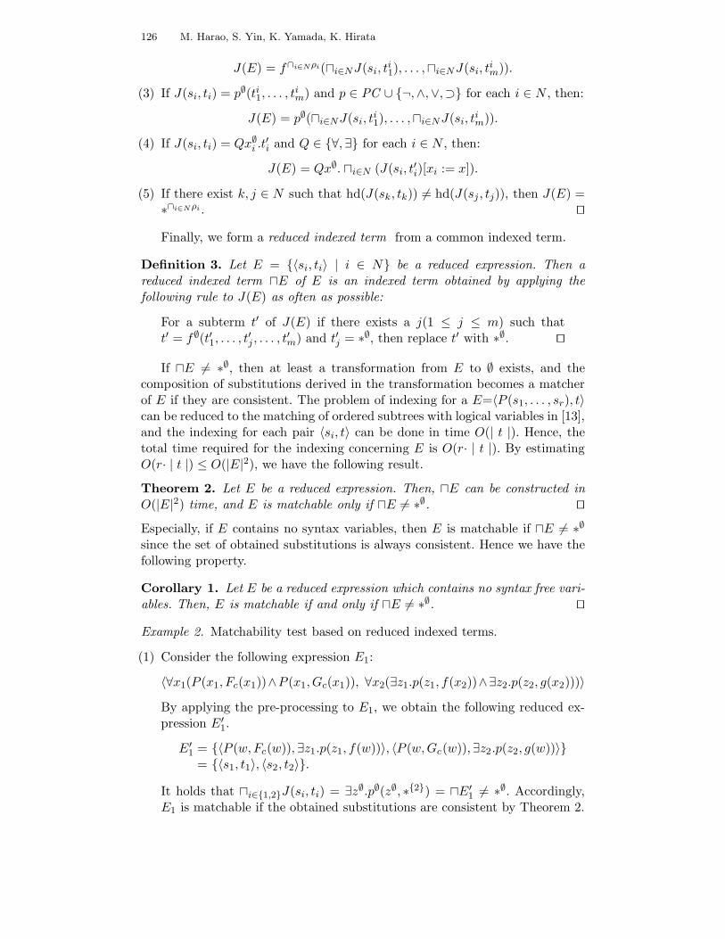
126 M. Harao, S. Yin, K. Yamada, K. Hirata
J(E) = f∩i∈Nρi(⊓i∈NJ(si, ti1), . . . ,⊓i∈NJ(si, t
im)).
(3) If J(si, ti) = p∅(ti1, . . . , tim) and p ∈ PC ∪ ¬,∧,∨,⊃ for each i ∈ N , then:
J(E) = p∅(⊓i∈NJ(si, ti1), . . . ,⊓i∈NJ(si, t
im)).
(4) If J(si, ti) = Qx∅i .t′i and Q ∈ ∀,∃ for each i ∈ N , then:
J(E) = Qx∅. ⊓i∈N (J(si, t′i)[xi := x]).
(5) If there exist k, j ∈ N such that hd(J(sk, tk)) 6= hd(J(sj , tj)), then J(E) =∗∩i∈N ρi . ⊓⊔
Finally, we form a reduced indexed term from a common indexed term.
Definition 3. Let E = 〈si, ti〉 | i ∈ N be a reduced expression. Then areduced indexed term ⊓E of E is an indexed term obtained by applying thefollowing rule to J(E) as often as possible:
For a subterm t′ of J(E) if there exists a j(1 ≤ j ≤ m) such thatt′ = f∅(t′1, . . . , t
′j , . . . , t
′m) and t′j = ∗∅, then replace t′ with ∗∅. ⊓⊔
If ⊓E 6= ∗∅, then at least a transformation from E to ∅ exists, and thecomposition of substitutions derived in the transformation becomes a matcherof E if they are consistent. The problem of indexing for a E=〈P (s1, . . . , sr), t〉can be reduced to the matching of ordered subtrees with logical variables in [13],and the indexing for each pair 〈si, t〉 can be done in time O(| t |). Hence, thetotal time required for the indexing concerning E is O(r· | t |). By estimatingO(r· | t |) ≤ O(|E|2), we have the following result.
Theorem 2. Let E be a reduced expression. Then, ⊓E can be constructed inO(|E|2) time, and E is matchable only if ⊓E 6= ∗∅. ⊓⊔
Especially, if E contains no syntax variables, then E is matchable if ⊓E 6= ∗∅
since the set of obtained substitutions is always consistent. Hence we have thefollowing property.
Corollary 1. Let E be a reduced expression which contains no syntax free vari-ables. Then, E is matchable if and only if ⊓E 6= ∗∅. ⊓⊔
Example 2. Matchability test based on reduced indexed terms.
(1) Consider the following expression E1:
〈∀x1(P (x1, Fc(x1))∧P (x1, Gc(x1)), ∀x2(∃z1.p(z1, f(x2))∧∃z2.p(z2, g(x2)))〉
By applying the pre-processing to E1, we obtain the following reduced ex-pression E′
1.
E′1 = 〈P (w,Fc(w)),∃z1.p(z1, f(w))〉, 〈P (w,Gc(w)),∃z2.p(z2, g(w))〉
= 〈s1, t1〉, 〈s2, t2〉.
It holds that ⊓i∈1,2J(si, ti) = ∃z∅.p∅(z∅, ∗2) = ⊓E′1 6= ∗
∅. Accordingly,E1 is matchable if the obtained substitutions are consistent by Theorem 2.

Second Order Schema Matching 127
(2) Consider the following expression E2 which contains no syntax free variables:
E2 =
〈∀x1.((P (x1, Fc(x1)) ∧ P (x1, Gc(x1))) ⊃ P (f(x1), x1)),∀x2.((∃z1.p(z1, f(x2)) ∧ ∃z2.p(z2, g(x2))) ⊃ ∃z3.p(z3, f(x2)))〉
.
Firstly, we apply the pre-processing to E2. Then we have the followingreduced expression E′
2.
E2 ⇒
〈(P (w,Fc(w)) ∧ P (w,Gc(w))) ⊃ P (Ff (w), w),
(∃z1.p(z1, f(w)) ∧ ∃z2.p(z2, g(w))) ⊃ ∃z3.p(z3, f(w)))〉
⇒
〈P (w,Fc(w)) ∧ P (w,Gc(w)), ∃z1.p(z1, f(w)) ∧ ∃z2.p(z2, g(w))〉,〈P (Ff (w), w), ∃z3.p(z3, f(w))〉
⇒
〈P (w,Fc(w)), ∃z1.p(z1, f(w))〉,〈P (w,Gc(w)), ∃z2.p(z2, g(w))〉,〈P (Fc(w), w), ∃z3.p(z3, f(w))〉
=
〈s1, t1〉,〈s2, t2〉,〈s3, t3〉
= E′
2
.
Next, we apply the projection point indexing to E′2. The indexed terms@are
given as follows:
J(s1, t1) = ∃z∅1 .p∅(z∅1 , f
2(w1)), J(s2, t2) = ∃z∅2 .p∅(z∅2 , g
2(w1)),
J(s3, t3) = ∃z∅3 .p∅(z∅3 , f
1(w2)).
By Definition 2, it holds that ⊓i∈1,2,3J(si, ti) = ∃z∅.p∅(z∅, ∗∅). By Defini-
tion 3, it holds that ⊓E′2 = ∗∅. Hence, E is not matchable by Corollary 1.
⊓⊔
4 Matcher Derivation Algorithm
4.1 A general matcher derivation algorithm
In this section we study algorithms of deriving any matchers of E from a givencommon reduced indexed term ⊓E. Intuitively, projection rules can be appliedto the positions of ⊓E whose index set ρ is not ∅, and imitation rules can beapplied to any positions of ⊓E which are not ⋆.
Definition 4. Let E be an expression such that 〈si, ti〉 | 1 ≤ j ≤ m,wherehd(si) = P for any i(1 ≤ i ≤ m). The set of substitutions S⊓E for E is definedinductively as follows.
(1) ⊓E = cρ : S⊓E = λvn.c ∪ λvn.vj | j ∈ ρ.(2) ⊓E = ⋆ρ : S⊓E =λvn.vj | j ∈ ρ.(3) ⊓E = fρ(⊓E1, . . . ,⊓Em) :
S⊓E=λvn.f(t1, . . . , tm) | λvn.ti ∈ S⊓Ei, 1 ≤ i ≤ m ∪ λvn.vj | j ∈ ρ. ⊓⊔
A matcher derivation term of E is a subterm of a reduced indexed term ⊓Eformed by deleting the descendant of every node to which a projection rule ischosen and the choiced index is labelled to each node of it. In case of ⊓E =p∅(f1,2(c3,4⋆5,6)), the terms p∅(f1), p∅(f∅(c∅, ⋆5)) and p∅(f∅(c4, ⋆5))are examples of matcher derivation terms of ⊓E. A atcher derivation termspecifies a substitution θ ∈ [H := t] | t ∈ S⊓E.
Note that the substitutions for syntax free variables arise only when pro-jection rules are applied. Accordingly, consistency check is required only whenprojection rules are applied.

128 M. Harao, S. Yin, K. Yamada, K. Hirata
Theorem 3. Let E be an expression and let ⊓E be its reduced indexed term.Then each consistent θ ∈ [H := t] | t ∈ S⊓E is a matcher of E. ⊓⊔
Corollary 2. Let E be an expression which contain no syntax free variablesand let ⊓E be its reduced indexed term. Then each θ ∈ [H := t] | t ∈ S⊓E isa matcher of E. ⊓⊔
Example 3. Matcher derivation from S⊓E
(1) Let E be an expression such that
E =
〈H(w,Fc(xa, w)), f(a,w)〉,〈H(xa, Fc(xa, xb)), f(a, b)〉,〈H(xa, Fc(xa, xc)), f(a, c)〉
.
Then ⊓E = f2(a∅, w1). The derivation terms of ⊓E are f∅(a∅, w1) andf2. Hence, we have the following substitutions:
θ1 = [H := λv1v2.f(a, v1), xa := b, xa := c],θ2 = [H := λv1v2.v2, Fc := λv1v2.f(v1, v2), xa := a].
Here, θ2 is a consistent matcher, but θ1 is not.
(2) Let E2 be the expression in Example2. Then ⊓E2 = ∃z∅.p∅(z∅, ∗2). In thiscase, the derivation term of E2 is uniquely defined as ∃z∅.p∅(z∅, ∗2). Hencewe have the following matcher. θ = [P := λv1v2.∃z.p(z, v2)]. ⊓⊔
A matcher derivation term is given by choosing rules and indices from re-duced indexed terms. The efficiency of the matching strongly depend on thischoosing procedure. We introduce a preference order ≻od into SE such that ifr1 ≻od r2, then r1 is chosen in preference to r2, and denote the ordered setby (SE,≻od). A strategy which derives matchers according to a preference or-der ≻od is called od-strategy, and a procedure which is based on od-strategy isdenoted by Matchod. A general procedure of Matchod is given as follows:
Algorithm Matchod :Input: E=〈P (sj), tj〉 | 1 ≤ j ≤ mOutput: Matchers of Ebegin(1)Pre-process E to a reduced expression E′;(2)Derive the reduced indexed term ⊓E;
If ⊓E = ⋆∅ then output fail;else
(3) While a possible matcher derivation term exists do;(3-1)Choose a possible matcher derivation term under od-strategy;(3-2)Derive substitutions according to the chosen matcher derivation term;(3-3)Check the consistency of the obtained substitutions;If consistent then output the substitutions;
end
As a basic preference order, we introduce the imitation preference order.

Second Order Schema Matching 129
Definition 5. The imitation preference order denoted by ≻I and the orderedset (S⊓E,≻I) are defined inductively as follows:
(1) ⊓E = cρ : (S⊓E ,≻I) = λvn.c ≻I λvn.v1 ≻I . . . ≻I λvn.v|ρ|.(2) ⊓E = ⋆ρ : (S⊓E ,≻I) = λvn.v1 ≻I . . . ≻I λvn.v|ρ|.(3) ⊓E = fρ(S⊓E1, . . . , S⊓Em): (S⊓E,≻I) =λvn.f(t1, . . . , tm) | λvn.ti ∈ (S⊓Em ,≻I) ≻I λvn.v1 ≻I . . . ≻I λvn.v|ρ|.
⊓⊔
Theorem 4. MatchI is sound and complete, that is, it derives any matchersof E. ⊓⊔
Especially, if E contains no syntax free variables, then the consistency check (3-3) is not necessary. Hence, for each choice in (3-1), MatchI derives a consistentmatcher.
Example 4. Let E be an expression such that 〈P (w,w,Fc(w), xc, xc), p(f(w), a)〉.Then ⊓E = p∅(f3(⋆1,2), a4,5), andMatchI derives the following 9 matchersin this order.
(1)[P := λv1v2v3v4v5.p(f(v1), a)](2)[P := λv1v2v3v4v5.p(f(v2), a)],(3)[P := λv1v2v3v4v5.p(f(v1), v4), xc := a],(4)[P := λv1v2v3v4v5.p(f(v1), v5), xc := a](5)[P := λv1v2v3v4v5.p(f(v2), v4), xc := a](6)[P := λv1v2v3v4v5.p(f(v2), v5), xc := a](7)[P := λv1v2v3v4v5.p(v3, a), Fc := λv.f(v)](8)[P := λv1v2v3v4v5.p(v3, v4), Fc := λv.f(v), xc := a](9)[P := λv1v2v3v4v5.p(v3, v5), Fc := λv.f(v), xc := a]
4.2 Efficiently Computable Predicate Schema Matching Classes
There exist one imitation rule and | ρ | projection rules which can be appliedto positions indexed as cρ or fρ(· · · ). Hence, the number of matcher derivationterms increases in exponential as for the number of such positions. It is essentialfor designing an efficient matching algorithm to suppress this combinationalexplosion.
One of the reasons of the increase of the size of ρ is the occurrence countof identical terms in arguments of schemas. For example, in Example 4, thesame symbols w, xc occur twice in the schema variable P . Hence, there exist4 combinations as for w, xc to form matcher derivation terms. However, it ismeaningless to derive matchers for all such combinations. In order to suppresssuch meaningless combinations, we restrict the occurrence count of each termin an atom to be at most one. From this viewpoint, we introduce the conditionof simplex.
For a position indexed as ⋆ρ, we have to apply projection rules. The size ofρ depend on the occurrence count of each bound variable w in an atom. For ex-ample, let E be 〈P (w,Fc(w)), p(f(w), a, b)〉. Then, ⊓E=p∅(f2(w1), a∅, b∅),and 2 matcher derivation terms exist. If we restrict the occurrence count of w
130 M. Harao, S. Yin, K. Yamada, K. Hirata
up to one, then the matcher derivation term is decided uniquely. For example,in case of 〈P (w,Fc(xc)), p(f(w), a, b)〉, its matcher derivation term is decideduniquely as p(f∅(w1), a∅, b∅). From this viewpoint, we introduce the conditionof linear.
The existence of bound variables in each argument of any atoms reducesthe indeterminacy of choosing rules. For example, let E be an expression suchthat
〈P (xc, yc), p(a, b)〉, 〈P (yc, xc), p(a, c)〉.
Then ⊓E = p∅(a1,2, ⋆1,2). For ⋆1,2, there exist 2 possible projections. Onthe other hand, in case of
〈P (xc, yc), p(a, b)〉, 〈P (yc, xc), p(a, c)〉 〈P (w, xc)), p(a,w)〉
,
⊓E = f∅(a2, ⋆1), and the index set of the position ⋆ is decided uniquely.Thus, for a position ⋆ρ, if there exists a sj
i (1 ≤ j ≤ m) for each i ∈ ρ which con-tains bound variables, that is, the position ⋆ is dominated with bound variables,then the matcher derivation term is uniquely decided. From this viewpoint, weintroduce the condition of dominated.
Definition 6. Let 〈P (sj1, . . . , s
jr), tj〉 | 1 ≤ j ≤ m be a reduced expression of
〈Φ, φ〉. Then
(1) An atom P (sj1, . . . , s
jr) is simplex if it contains bound variables, then sj
i 6=
sji′(1 ≤ i, i
′ ≤ r) holds for any j(1 ≤ j ≤ m). A schema Φ is simplex if eachatom of Φ is simplex.
(2) An atom P (sj1, . . . , s
jr) is linear if the occurrence count of each bound variable
of the atom is at most one. A schema Φ is linear if each atom of Φ is linear.
(3) A set of atoms P (sj1, . . . , s
jr) | (1 ≤ j ≤ m) is dominated if sj
i 6= sj′
i (1 ≤
j, j′ ≤ m) holds for some i(1 ≤ i ≤ r), then at least a s ∈ sji | 1 ≤ j ≤ m
contains bound variables. A schema Φ is dominated if each atom set of Φwith a same head is dominated. ⊓⊔
Example 5. Let Φ1, Φ2, Φ3 be schemas such that:
Φ1 = ∀xy.P (x, y, xc, yc) ⊃ P (xc, yc, xc, yc)Φ2 = ∀x.P (x, Fc(x), xc, yc) ⊃ P (xc, xc, xc, xc)Φ3 = ∀xy.P (x, y, xc, xc) ⊃ P (xc, yc, xc, xc)
Then Φ1 is simplex, dominated and linear. Φ2 is simplex, but is not dominatedsince the 4th argument of its atoms are different (yc 6= xc) but no boundvariables occurs in the 4th argument of both atoms. Further Φ2 is not linearsince x occurs twice in ∀x.P (x, f(x), xc, yc). Φ3 is not simplex since xc occurstwice in ∀x.P (x, f(x), xc, xc), but is dominated and linear. ⊓⊔
A schema Φ is called s-l-d if it satisfies all the conditions of simplex, dom-inated and linear. Let E = 〈si, ti〉 | i ∈ N be a reduced expression obtainedfrom a s-l-d schema Φ, and let J(E) be the common indexed term of E. Assumethat ⋆ρ be a position of J(E). If ⋆ρ is derived by hd(J(sk, tk)) 6= hd(J(sj , tj)
Second Order Schema Matching 131
and skl = sj
l holds for any k, j ∈ N where sk = P (sk1, . . . , s
kr ) ,sj = P (sj
1, . . . , sjr)
and l ∈ ρ, then the substitutions obtained by applying projection rules to theposition ,i.e.,λvn.vl, l ∈ ρ, are inconsistent. Therefore, this matching fails. Forthis reason, for the case of s-l-d schema, we modify the definition of commonindexed term (Definition 2(5)) as follows:
(5)’ If there exist k, j ∈ N such that hd(J(sk, tk)) 6= hd(J(sj , tj)), then
J(E) = ∗∩i∈N ρi−α, where α = l | skl = sj
l ,∀k, j ∈ N and sk = P (sk1 , . . . , s
kr),
sj = P (sj1, . . . , s
jr).
From the condition of linear, the relation | ρ |≤ 1 holds for any ⋆ρ. Accord-ingly, if Φ is s-l-d schema, then the positions to which projection rules must beapplied are uniquely specified.
Example 6. Matching for s-l-d schemas.
(1) Let E1 = 〈P (xc, yc), p(a)〉, 〈P (xc, zc), p(b)〉, 〈P (xc, w), p(c)〉. Then we have⊓E1=p
∅(⋆∅) instead of p∅(⋆1). Finally we have the reduced indexed term ⋆∅,and therefore this matching fails. We can ascertain that the substitutions [xc :=a, xc := b, xc := c] obtained by applying the projection λuv.u to the ⋆ positionare inconsistent.
(2) Let E2 = 〈P (Fc(xc)), p(f(a))〉, 〈H(Fc(xc)), p(f(b))〉. Then we have ⊓E2=⋆∅
by reducing from p∅(f1(⋆∅)). Hence this matching fails.
(3) Let E3 = 〈P (Fc(xc)), p(f(a))〉, 〈P (Fc(yc)), p(f(b))〉, 〈P (Fc(w)), p(f(w))〉.Then ⊓E3 =p∅(f1), and E3 is matchable. The matcher is [P := λu.p(u), Fc :=λv.f(v), xc := a, yc := b]. ⊓⊔
Let t = ⊓E be the reduced indexed term of E obtained from a s-l-d schema.Then a strategy which uses only imitation rules for the positions indexed as cρ
or fρ(· · · ) is called strong imitation preference. The matching MatchS basedon this strong imitation preference strategy is defined as follows.
Definition 7. s-l-d schema matching.
(1) ⊓E = cρ : (Ss⊓E ,≻) = λvn.c.
(2) ⊓E = ⋆ρ : (Ss⊓E ,≻) =λvn.vj,where j ∈ ρ (| ρ |≤ 1).
(3) ⊓E = fρ(S⊓E1, . . . , S⊓Em) : (Ss⊓E ,≻)=λvn.f(t1, . . . , tm) | λvn.ti ∈ S⊓Em.
⊓⊔
Next, we estimate the time complexity of MatchS . Let E be a reducedexpression. The procedures in (3) are linear except for (3-1). However, in thecase of the s-l-d schema matching, this procedure (3-1) becomes linear since theprojection position set is uniquely decided and | ρ |≤ 1.
The projection position indexing procedure is computable in time O(r· | t |)as stated in Theorem2. Especially, in the case of schema matching, we canassume that | t |≤ (k | si |) holds for some fixed k ∈ N . Accordingly, in thiscase, the complexity of the matching becomes O(| E |). Therefore, in most ofthe cases, the s-l-d schema matching runs almost in linear time. Thus, we havethe following results.

132 M. Harao, S. Yin, K. Yamada, K. Hirata
Theorem 5. Let Φ be a s-l-d schema and E be a reduced expression for some〈Φ, φ〉. Then MatchS derives a unique matcher of E almost in linear time if Eis matchable. ⊓⊔
Example 7. Let E be a matching pair 〈Φ,ϕ〉 such that
Φ = P (xc) ∧ ∀x.(P (x) ⊃ P (Fc(x))) ⊃ P (Fc(Fc(xc))).φ = (p(0) ∧ q(0)) ∧ ∀x.(p(x) ∧ q(x) ⊃ p(suc(x)) ∧ suc(x))
⊃ (p(suc(suc(0))) ∧ q(suc(suc(0)))
At first, we have the following reduced expression:
E =
〈P1(xc), p(0)〉 〈P1(w), p(w) 〉,〈P1(Fc(w)), p(suc(w))〉, 〈P1(Fc(Fc(xc))), p(suc(suc(0)))〉〈P2(xc), q(0)〉 〈P2(w), q(w) 〉〈P2(Fc(w)), q(suc(w))〉, 〈P2(Fc(Fc(xc))), q(suc(suc(0)))〉
Then we have the reduced indexed terms such that :
⊓E1 = p∅(⋆1), ⊓E2 = q∅(⋆1).
Hence, we have the substitutions such that
P1 := λu1.p(u1), P2 := λu2.q(u2), Ff := λv.suc(v), xc := 0.
Finally, we have the matcher [P := λu1u2.p(u1) ∧ q(u2), Fc := λv.suc(v), xc :=0. ⊓⊔
5 Discussions and Conclusion
We have discussed in this paper the second order predicate schema match-ing motivating to apply it to the schema guided theorem proving. We pro-posed an algorithm MatchI which pre-checks the projection positions andshowed an efficiently computable class characterized by the conditions sim-plex,linear and dominated exists. Though the conditions seem to be too re-strictive, these restrictions do not reduce the expressive power of schemas. Forexample,∀x.P (x, xc, Fc(yc)) matches with formulas containing the bound vari-able x such that
∀x.p(x, a, f(a), g(x)),∀x.(∃y.q(x, y, a, f(a), b, f(x), g(y)),∀x.(∃y.p(x, f(y), a, g(x)) ∧ ∀y∃z.q(x, y, z, a, b, f(a), g(b))
. . . . . .
The conditions of dominated are motivated from the provability of schemas.Let Φ be a schema expressed in sequent such that
∀x∀y.P (xa, x, Fc(y))⇒ P (xa, xb, xc).
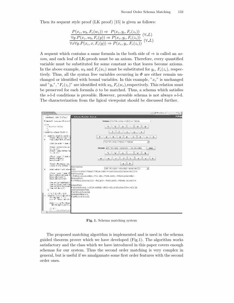
Second Order Schema Matching 133
Then its sequent style proof (LK proof) [15] is given as follows:
P (xc, wb, Fc(wc))⇒ P (xc, yc, Fc(zc))
∀y.P (xc, wb, Fc(y))⇒ P (xc, yc, Fc(zc))(∀ L)
∀x∀y.P (xc, x, Fc(y))⇒ P (xc, yc, Fc(zc))(∀ L)
A sequent which contains a same formula in the both side of ⇒ is called an ax-iom, and each leaf of LK-proofs must be an axiom. Therefore, every quantifiedvariable must be substituted for some constant so that leaves become axioms.In the above example, wb and Fc(wc) must be substituted for yc, Fc(zc), respec-tively. Thus, all the syntax free variables occurring in Φ are either remain un-changed or identified with bound variables. In this example, ”xc” is unchangedand ”yc”, ”Fc(zc)” are identified with wb, Fc(wc),respectively. This relation mustbe preserved for each formula φ to be matched. Thus, a schema which satisfiesthe s-l-d conditions is provable. However, provable schema is not always s-l-d.The characterization from the ligical viewpoint should be discussed further.
Fig. 1. Schema matching system
The proposed matching algorithm is implemented and is used in the schemaguided theorem prover which we have developed (Fig.1). The algorithm workssatisfactory and the class which we have introduced in this paper covers enoughschemas for our system. Thus the second order matching is very complex ingeneral, but is useful if we amalgamate some first order features with the secondorder ones.
134 M. Harao, S. Yin, K. Yamada, K. Hirata
References
1. L. D. Baxter. The complexity of unification. PhD thesis, Department of Computer Science,University of Waterloo, 1977.
2. B. Brock, S. Cooper, and W. Pierce. Analogical reasoning and proof discovery. LNCS,No.310:454–468, 1988.
3. R. Curien, Z. Qian, and H. Shi. Efficient second order matching. In RTA 96(RewritingTechniques and Application), pages 317–331, 1996.
4. M. R. Donat and L. A. Wallen. Learning and applying generalised sotutions using higherorder resolution. LNCS, No.310:41–60, 1988.
5. G. Dowek. Third order matching is decidable. In 7th Annual IEEE Symposium on Logicin Computer Science, pages 2–10, 1992.
6. P. Flener. Logic program synthesis from incomplete information. Kluwer Academic Press,1995.
7. M. Harao. Proof discovery in lk system by analogy. In LNCS(Proc. of the 3rd AsianComputing Science Conference), volume 1345, pages 197–211, 1997.
8. M. Harao and K. Iwanuma. Complexity of higher-order unification algorithm. Society forSoftware Science and Technology, No.8:41–53, 1991. In Japanese.
9. M. Harao, K. Yamada, and K. Hirata. Efficient second order predicate matching algo-rithm. In Proc. Korea-Japan Joint Workshop on Algorithm and Computations, pages31–39, 1999.
10. K. Hirata, K. Yamada, and M. Harao. Tractable and intractable second-order matchingproblems. Journal of Symbolic Computation, 37:611–628, 2004.
11. G. P. Huet. A unification algorithm for typed λ-calculus. Journal of Theoretical ComputerScience, 1:27–57, 1975.
12. G. P. Huet and B. Lang. Proving and applying program transformations expressed withsecond-order patterns. Acta Informatica, 11:31–55, 1978.
13. P. Kilpelainen. Tree Matching Problems with Applications to Structured Text Databases.PhD thesis, University of Helsinki Department of Computer Science, 1992.
14. D. A. Miller. A logic programming language with lambda-abstraction function variables,and simple unification. J. of Logic and Computations, 1(4):494–536, 1991.
15. A. S. Troelstra and H. Schwichtenberg. Basic proof Theory. Cambridge University Press,1996.
16. K. Yamada, K. Hirata, and M. Harao. Schema matching and its complexity. Trans.IEICE, J82-D-I:1307–1316, 1999. In Japanese.
17. K. Yamada, S. Yin, M. Harao, and K. Hirata. Development of an analogy-based genericsequent style automatic theorem prover amalgamated with interactive proving. In Proc.of IWIL’05 (the International Workshop on the Implementation of Logics 2005), 2005.
Panel Discussion: 20 Years After OBJ2
Organized by Kokichi Futatsugi
A memorable paper on OBJ2 [1] was published in the year 1985 in theproceedings of the Twelfth POPL. OBJ2 was an algebraic specification languagedesigned and implemented from 1983 to 1984 by the four authors of the paperat SRI International in Menlo Park, California. OBJ2 was a novel executableformal specification language, and it had many new features its predecessorlanguages were lacking.
Although the definitive implementation of OBJ2 is OBJ3, which has beenwidely used as the latest OBJ language, almost all important language featureswere defined in OBJ2. The novel features of OBJ2 such as powerful modulesystem, order sorted signature, rewriting modulo equational theories (A/C/I),evaluation strategy (E-strategy), etc. have influenced the designs of many lan-guages in the last 20 years. Those languages include, at least:
BOBJ (http://www-cse.ucsd.edu/groups/tatami/bobj/)CafeOBJ (http://www.ldl.jaist.ac.jp/cafeobj/)CASL (http://www.cofi.info/CASL.html)ELAN (http://elan.loria.fr/)Maude (http://maude.cs.uiuc.edu/)
The four authors of the OBJ2 paper share the luck of participating RDP2005exactly 20 yeas after the paper was published. All of the four have been frequentinternational travelers and attended many international conferences / sympo-siums / workshops, but it is really rare to have this kind of coincidence. Thepanel discussion of 20 Years After OBJ2 is organized by making use of thisprecious chance for discussing the future possibilities of algebraic specificationlanguages, rewriting techniques, rewriting logic, behevioral / observational spec-ification, etc. based on 20 years of experiences after OBJ2.
Panelists include the following four authors of the OBJ2 paper and one ortwo more persons.
Kokichi FutatsugiJAIST (Japan Advance Institute of Science and Technology)[email protected]
Joseph GoguenUniversity of California at San [email protected]
Jean-Pierre JouannaudEcole [email protected]
Jose MeseguerUniversity of Illinois at [email protected]
135

136 Organized by Kokichi Futatsugi
References
1. K. Futatsugi, J.A. Goguen, J.P. Jouannaud and J. Meseguer. Principles of OBJ2. In:Conference Record of the Twelfth Annual ACM Symposium on Principles of ProgrammingLanguages, New Orleans, Louisiana, January 1985 (POPL85), ACM (1985) 52-66.

Author Index
Anantharaman, Siva, 93
Bakewell, Adam, 25
Chabin, Jacques, 41Chen, Jing, 41Cheney, James, 105Chevalier, Yannick, 63
Futatsugi, Kokichi, 135
Goguen, Joseph, 135
Harao, Masateru, 121Hirata, Kouichi, 121
Jouannaud, Jean-Pierre, 135
Kfoury, Assaf J., 25Kutsia, Temur, 77
Lynch, Christopher, 47
Marin, Mircea, 77Meseguer, Jose, 135Morawska, Barbara, 47
Narendran, Paliath, 93Niehren, Joachim, 1
Planque, Laurent, 1
Rety, Pierre, 41Rusinowitch, Michael, 63, 93
Talbot, Jean-Marc, 1Tison, Sophie, 1
Yamada, Keizo, 121Yin, Shuping, 121
137