1997 by Jay H. L e, Jin Ho on Choi, and Kwang So on L · e, Jin Ho on Choi, and Kwang So on L In v...

c 1997 by Jay H. Lee, Jin Hoon Choi, and Kwang Soon Lee

Part III

BACKGROUND FOR ADVANCED

ISSUES

1


Contents

1 BASICS OF LINEAR ALGEBRA 5

1.1 VECTORS . . . . . . . . . . . . . . . . . . . . . . . . . . . . . . . . . . . . 5

1.2 MATRICES . . . . . . . . . . . . . . . . . . . . . . . . . . . . . . . . . . . . 11

1.3 SINGULAR VALUE DECOMPOSITION . . . . . . . . . . . . . . . . . . . . 23

2 BASICS OF LINEAR SYSTEMS 30

2.1 STATE SPACE DESCRIPTION . . . . . . . . . . . . . . . . . . . . . . . . . 30

2.2 FINITE IMPULSE RESPONSE MODEL . . . . . . . . . . . . . . . . . . . . 38

2.3 TRUNCATED STEP RESPONSE MODEL . . . . . . . . . . . . . . . . . . 41

2.4 REACHABILITY AND OBSERVABILITY . . . . . . . . . . . . . . . . . . 44

2.5 STATIC STATE FEEDBACK CONTROLLER AND STATE ESTIMATOR 47

3 BASICS OF OPTIMIZATION 52

3.1 INTRODUCTION . . . . . . . . . . . . . . . . . . . . . . . . . . . . . . . . 52

3.2 UNCONSTRAINED OPTIMIZATION PROBLEMS . . . . . . . . . . . . . 55

3.3 NECESSARY CONDITION OF OPTIMALITY FOR CONSTRAINED OP-

TIMIZATION PROBLEMS . . . . . . . . . . . . . . . . . . . . . . . . . . . 59

3.4 CONVEX OPTIMIZATION . . . . . . . . . . . . . . . . . . . . . . . . . . . 67

3.5 ALGORITMS FOR CONSTRAINED OPTIMIZATION PROBLEMS . . . . 71

2


4 RANDOM VARIABLES 79

4.1 INTRODUCTION . . . . . . . . . . . . . . . . . . . . . . . . . . . . . . . . 79

4.2 BASIC PROBABILITY CONCEPTS . . . . . . . . . . . . . . . . . . . . . . 81

4.2.1 PROBABILITY DISTRIBUTION, DENSITY: SCALAR CASE . . . 81

4.2.2 PROBABILITY DISTRIBUTION, DENSITY: VECTOR CASE . . . 83

4.2.3 EXPECTATION OFRANDOMVARIABLES ANDRANDOMVARI-

ABLE FUNCTIONS: SCALAR CASE . . . . . . . . . . . . . . . . . 86

4.2.4 EXPECTATION OFRANDOMVARIABLES ANDRANDOMVARI-

ABLE FUNCTIONS: VECTOR CASE . . . . . . . . . . . . . . . . . 87

4.2.5 CONDITIONAL PROBABILITY DENSITY: SCALAR CASE . . . . 92

4.2.6 CONDITIONAL PROBABILITY DENSITY: VECTOR CASE . . . 97

4.3 STATISTICS . . . . . . . . . . . . . . . . . . . . . . . . . . . . . . . . . . . 99

4.3.1 PREDICTION . . . . . . . . . . . . . . . . . . . . . . . . . . . . . . 99

4.3.2 SAMPLE MEAN AND COVARIANCE, PROBABILISTIC MODEL 100

5 STOCHASTIC PROCESSES 102

5.1 BASIC PROBABILITY CONCEPTS . . . . . . . . . . . . . . . . . . . . . . 102

5.1.1 DISTRIBUTION FUNCTION . . . . . . . . . . . . . . . . . . . . . . 102

5.1.2 MEAN AND COVARIANCE . . . . . . . . . . . . . . . . . . . . . . 103

5.1.3 STATIONARY STOCHASTIC PROCESSES . . . . . . . . . . . . . 103

5.1.4 SPECTRA OF STATIONARY STOCHASTIC PROCESSES . . . . . 104

5.1.5 DISCRETE-TIME WHITE NOISE . . . . . . . . . . . . . . . . . . . 106

5.1.6 COLORED NOISE . . . . . . . . . . . . . . . . . . . . . . . . . . . . 106

5.1.7 INTEGRATEDWHITE NOISE ANDNONSTATIONARY PROCESS-

ES . . . . . . . . . . . . . . . . . . . . . . . . . . . . . . . . . . . . . 108

3


5.1.8 STOCHASTIC DIFFERENCE EQUATION . . . . . . . . . . . . . . 109

5.2 STOCHASTIC SYSTEM MODELS . . . . . . . . . . . . . . . . . . . . . . . 111

5.2.1 STATE-SPACE MODEL . . . . . . . . . . . . . . . . . . . . . . . . . 111

5.2.2 INPUT-OUTPUT MODELS . . . . . . . . . . . . . . . . . . . . . . . 114

6 STATE ESTIMATION 116

6.1 LINEAR OBSERVER STRUCTURE . . . . . . . . . . . . . . . . . . . . . . 117

6.2 POLE PLACEMENT . . . . . . . . . . . . . . . . . . . . . . . . . . . . . . . 119

6.3 KALMAN FILTER . . . . . . . . . . . . . . . . . . . . . . . . . . . . . . . . 120

6.3.1 KALMAN FILTER AS THE OPTIMAL LINEAR OBSERVER . . . 121

6.3.2 KALMAN FILTER AS THE OPTIMAL ESTIMATOR FOR GAUS-

SIAN SYSTEMS . . . . . . . . . . . . . . . . . . . . . . . . . . . . . 123

7 SYSTEM IDENTIFICATION 127

7.1 PROBLEM OVERVIEW . . . . . . . . . . . . . . . . . . . . . . . . . . . . . 127

7.2 PARAMETRIC IDENTIFICATION METHODS . . . . . . . . . . . . . . . 128

7.2.1 MODEL STRUCTURES . . . . . . . . . . . . . . . . . . . . . . . . . 129

7.2.2 PARAMETER ESTIMATION VIA PREDICTION ERROR MINI-

MIZATION . . . . . . . . . . . . . . . . . . . . . . . . . . . . . . . . 134

7.2.3 PARAMETER ESTIMATION VIA STATISTICAL METHODS . . . 143

7.2.4 OTHER METHODS . . . . . . . . . . . . . . . . . . . . . . . . . . . 150

7.3 NONPARAMETRIC IDENTIFICATION METHODS . . . . . . . . . . . . . 151

7.3.1 FREQUENCY RESPONSE IDENTIFICATION . . . . . . . . . . . . 152

7.3.2 IMPULSE RESPONSE IDENTIFICATION . . . . . . . . . . . . . . 156

7.3.3 SUBSPACE IDENTIFICATION . . . . . . . . . . . . . . . . . . . . . 158

4


Chapter 1

BASICS OF LINEAR ALGEBRA

1.1 VECTORS

De�nition of Vector

Consider a CSTR where a simple exothermic reaction occurs:

A neat way to represent process variables, F;CA; T , is to stack

them in a column. 266666664

F

CA

T

377777775

5


De�nition of Vector (Continued)

In general, n tuples of numbers stacked in a column is called vector.

x =

2666666666664

x1

x2...

xn

3777777777775

Transpose of a Vector x:

xT = [x1 x2 � � � xn]

6


Basic Operations of Vectors

a: a scalar, x; y: vectors

Addition:

x + y =

2666666666664

x1

x2...

xn

3777777777775+

2666666666664

y1

y2...

yn

3777777777775=

2666666666664

x1 + y1

x2 + y2...

xn + yn

3777777777775

Scalar Multiplication:

ax = a

2666666666664

x1

x2...

xn

3777777777775=

2666666666664

ax1

ax2...

axn

3777777777775

7


Vector Norms

Norm is the measure of vector size.

p norms:

kxkp = (jx1jp + � � � + jxnjp)1

p 1 � p <1

kxk1 = maxijxij

Example:

kxk1 = jx1j + � � � + jxnjkxk2 =

rjx1j2 + � � � + jxnj2

kxk1 = maxfjx1j; � � � ; jxnjgkxk2 coincides with the length in Euclidean sense and, thus, is

called Eclidean norm. Throughout the lecture, k � k denotes k � k2.

8


Inner Product

Inner Product:

x � y = xTy = kxkkyk cos �+

x � y8>>>>><>>>>>:

> 0 if � is acute

= 0 if � is right

< 0 if � is obtuse

Note that two vectors x; y are orthogonal if xTy = 0

9


Linear Independence and Basis

a1; � � � ; am: scalars, x1; � � � ; xm: vectors

Linear Combination:

a1x1 + a2x2 + � � � + amxm

Span: Span of x1; � � � ; xm is the set of all linear combination of

them, which is a plane in Rn.

spanfx1; x2; � � � ; xmg = fx = a1x1 + a2x2 + � � � + amxmg

Linear Independence: fx1; � � � ; xmg is called linearly independent if

no one of them is in the span of others.

Basis of a Space (S): A set of linearly independent vectors

fx1; x2; � � � ; xmg such that S = spanfx1; x2; � � � ; xmg10


1.2 MATRICES

De�nition of Matrices

Let A be the linear mapping from a vector x to another vector y.

Then A is represented by a rectangular array of numbers:

A =

2666666666664

a11 a12 � � � a1n

a21 a22 � � � a2n... ... ... ...

am1 am2 � � � amn

3777777777775

that is called m� n-matrix.

Transpose of a Matrix A:

AT =

2666666666664

a11 a21 � � � am1a12 a22 � � � am2... ... ... ...

a1n a2n � � � amn

3777777777775

Conjugate Transpose of a Matrix A:

A� =

2666666666664

�a11 �a21 � � � �am1

�a12 �a22 � � � �am2... ... ... ...

�a1n �a2n � � � �amn

3777777777775

Notice that AT = A� for real matrices.

11


Basic Operation of Matrices

a: a scalar, A;B: matrices

Addition:

A + B =

2666666666664

a11 a12 � � � a1n

a21 a22 � � � a2n... ... ... ...


3777777777775+

2666666666664

b11 b12 � � � b1n

b21 b22 � � � b2n... ... ... ...

bm1 bm2 � � � bmn

3777777777775

=

2666666666664

a11 + b11 a12 + b12 � � � a1n + b1n

a21 + b21 a22 + b22 � � � a2n + b2n... ... ... ...

am1 + bm1 am2 + bm2 � � � amn + bmn

3777777777775

Scalar Multiplication:

aA = a

2666666666664

a11 a12 � � � a1n

a21 a22 � � � a2n... ... ... ...


3777777777775=

2666666666664

aa11 aa12 � � � aa1n

aa21 aa22 � � � aa2n... ... ... ...

aam1 aam2 � � � aamn

3777777777775

12


Basic Operation of Matrices (Continued)

Matrix Multiplication:

AB =

2666666666664

a11 a12 � � � a1n

a21 a22 � � � a2n... ... ... ...


3777777777775

2666666666664

b11 b12 � � � b1lb21 b22 � � � b2l... ... ... ...

bn1 bn2 � � � bnl

3777777777775

=

2666666666664

Pni=1 a1ibi1

Pni=1 a1ibi2 � � � Pn

i=1 a1ibilPni=1 a2ibi1

Pni=1 a2ibi2 � � � Pn

i=1 a2ibil... ... ... ...

Pni=1 amibi1

Pni=1 amibi2 � � � Pn

i=1 amibil

3777777777775

13


Inverse of Square Matrices

Inverse of an n� n matrix A is an n� n matrix such that

AA�1 = A�1A = I

Theorem: An n� n matrix A has its inverse i� the columns of A

are linearly independent.

Suppose A de�nes a linear transformation:

y = Ax

Then the inverse of A de�nes the inverse transformation:

x = A�1y

14


Unitary Matrices

Matrix that rotates a vector without change of size is called unitary

matrix

Properties of Unitary Matrix:

U�U = I = UU�

15


Coordinate Transformation

z: a vector, fu; vg, fx; yg: coordinate systems

z = �w1u + �w2v = w1x + w2y ) [u v] �w = [x y]w

+�w = Tw; T = [u v]�1[x y]

In general, the representations of a vector in two di�erent

coordinate systems are related by an invertible matrix T :

�w = Tw

w = T�1 �w

16


Coordinate Transformation (Continued)

Representations of matrix in di�erent coordinates:

Suppose � = T �� and � = T ��. Then

� = A� ) T �� = AT �� ) �� = T�1AT ��

+�� = �A ��

where

�A = T�1AT

that is called the similarity transformation of A.

17


Eigenvalues and Eigenvectors

The eigenvalues of n� n matrix A are n roots of det(�I �A).

If � is an eigenvalue of A, 9 nonzero v such that

Av = �v

where v is called eigenvector.

18


Eigenvalue Decomposition

Let A 2 Rn�n. Suppose �i be eigenvalues of A such that

�1 � �2 � � � � � �n

Let

T = [v1; v2; � � � ; vn] 2 Rn�n

where vi denotes eigenvector of A associated with �i. If A has n

linearly independent eigenvectors,

A = T�T�1

where

� =

2666666666664

�1 0 � � � 0

0 �2 � � � 0... ... . . . ...

0 � � � 0 �n

3777777777775

Notice that � is simply the representation of A in the coordinate

system consists of eigenvectors.

19


Symmetric Matrices

A matrix A is called symmetric if

A = AT

Symmetric matrix is useful when we consider a quadratic form.

Indeed, given a matrix A,

xTAx = xTSx

where S is the symmetric matrix de�ned by

S =1

2(A + AT )

Positive De�niteness: A symmetric matrix A is positive de�nite if

xTAx > 0 8x 6= 0; x 2 Cn

Positive Semi-De�niteness: A symmetric matrix A is positive

semi-de�nite if

xTAx � 0

Theorem: A symmetric matrix A is positive de�nite i� all the

eigenvalues of A are positive.

20


Matrix Norms

A =

2666666666664

a11 a12 � � � a1n

a21 a22 � � � a2n... ... . . . ...


37777777777752 Cm�n

p norms:

jjjAjjjp = (Xi;jjai;jjp)

1

p 1 � p <1

jjjAjjj1 = maxi;j

jai;jjjjj � jjj2 is called Euclidean or Frobenius norm.

What is the di�erence between Cm�n and Cmn?

A matrix in Cm�n de�nes a linear operator from Cn to Cm;

y = Ax.

21


Matrix Norms (Continued)

Induced (or operator) p norms:

kAkp = supx6=0

kAxkpkxkp = max

kxk=1kAxkp 1 � p � 1

+

kykp = kAxkp � kAkpkxkp 8x 2 Cn

Examples:

p = 1:

kAk1 = maxj

mXi=1jai;jj

p = 2: spectral norm

kAk2 = [�max(ATA)]

1

2

p =1:

kAk1 = maxi

mXj=1

jai;jj

22


1.3 SINGULAR VALUE DECOMPOSITION

Singular Values and Singular Vectors

Singular values of an m� n matrix A are the square roots of

minfm;ng eigenvalues of A�A.

�(A) =r�(A�A)

Right singular vectors of a matrix A are the eigenvectors of A�A.

�(A)2v �A�Av = 0

Left singular vectors of a matrix A are the eigenvectors of AA�.

�(A)2u�AA�u = 0

��(A) = the largest singular value of A = maxkxk=1

kAxk = kAk2The largest possible size change of a vector by A.

�(A) = the smallest singular value of A = minkxk=1

kAxk

The smallest possible size change of a vector by A.

23


Singular Values and Singular Vectors (Continued)

Condition number: c(A) = �(A)��(A)

A�v = ��u

Av = � u

+�v (v): highest (lowest) gain input direction

�u (u): highest (lowest) gain observing direction

24


Singular Value Decomposition

Let A 2 Rm�n. Suppose �i be singular values of A such that

�1 � �2 � � � � � �p � 0; p = minfm;ng

Let

U = [u1; u2; � � � ; um] 2 Rm�m V = [v1; v2; � � � ; vn] 2 Rn�n

where ui; vj denote left and right orthonormal singular vectors of

A, respectively. Then

A = U�V �; � =

2664 �1 0

0 0

3775 =

pXi=1

�i(A)uiv�i

where

�1 =

2666666666664

�1 0 � � � 0

0 �2 � � � 0... ... � � � ...

0 0 � � � �p

3777777777775

Consider y = Ax. Then � is simply the representation of A when x

and y are represented in the coordinate systems consisting of right

and left singular vectors, respectively.

25


Singular Value Decomposition (Continued)

Example:

A =

2664 0:8712 �1:31951:5783 �0:0947

3775

+

U =1p2

2664 1 �11 1

3775 ; � =

2664 2 0

0 1

3775 ; V =

1

2

2664p3 1

�1 p3

3775

26


Principal Component Analysis

Given N n-dimensional vectors fx1; x2; � � � ; xNg, the principalvector p is

p = arg minkpk=1

NXi=1kxi � hxi; pipk2

= arg minkpk=1

NXi=1

�hxi; xii � 2hxi; pi2 + hxi; pi2hp; pi

�

= arg minkpk=1

NXi=1�hxi; pi

2

hp; pi = argmaxNXi=1

hxi; pi2hp; pi = argmax�(p)

where

�(p) =NXi=1

xTi ppTxi

pTp

27


Principal Component Analysis (Continued)

At the extremum,

0 =1

2

d�

dp=

NXi=1

xixTi p

pTp� NX

i=1

xTi ppTxip

(pTp)2

+

0 =NXi=1

xixTi p�

NXi=1

xTi ppTxi

pTpp = XXTp��p Singular Value Problem for X

where

X = [x1 x2 � � � xN ]; � =NXi=1

xTi ppTxi

(pTp)2

The SVD of X is

X = P�1

2V T = p1�1

2

1uT1 + � � � + pn�

1

2nu

Tn

where

P = [p1 p2 � � � pn]; V = [v1 v2 � � � vN ];� = [diag[�

1

2

i ] 0] 0 = XTXv � �v

�1

2

1 � � � � � �1

2n

The approximation of X using �rst m signi�cant principal vectors:

X � �X = �P ��1

2 �UT = p1�1

2

1uT1 + � � � + pm�

1

2mu

Tm

where

�P = [p1 p2 � � � pm]; � = diag[�1

2

i ]mi=1

�V = [v1 v2 � � � vm]28


Principal Component Analysis (Continued)

pTi X = pTi (p1�1

2

1uT1 + � � � + pn�

1

2nu

Tn ) = �

1

2

i uTi

+�P TX = �UT

+�X = �P �UT = �P �P TX

and the residual is

~X = X � �X = (I � �P �P T )X

29


Chapter 2

BASICS OF LINEAR SYSTEMS

2.1 STATE SPACE DESCRIPTION

State Space Model Development

Consider fundamental ODE model:

dxfdt

= f(xf ; uf)

yf = g(xf)

xf : state vector,

uf : input vector

yf : output vector

30


State Space Model Development (Continued)

+ linearization w.r.t. an equilibrium (�x; �u)

dxdt

=

df@xf

!ssx +

@f@uf

!ssu

y =

@g@xf

!ssx

where x = xf � �x, u = uf � �u.

+ discretization

x(k + 1) = Ax(k) + Buu(k)

y(k) = Cx(k)

31


State Space Description of Linear Systems

Consider the linear system described by the state equation:

x(k + 1) = Ax(k) +Bu(k)

y(k) = Cx(k)

Take z-Transformation

zX(z) = AX(z) +BU(z)

Y (z) = CX(z)

+Y (z) = C(zI �A)�1BU(z)

Solution to Linear System:

x(k) = Anx(0) +n�1Xi=0

An�i�1Bu(i)

32


Transfer Function

Consider the system described by transfer function:

Y (z)

U(z)=b1z

n�1 + b2zn�2 + � � � + bn

zn + a1zn�1 + � � � + an

Then a state space description of the system is

x(k + 1) = Ax(k) +Bu(k)

y(k) = Cx(k)

where

A =

266666666666666664

�a1 �a2 � � � �an�1 �an1 0 � � � 0 0

0 1 � � � 0 0... ... . . . ... ...

0 0 � � � 1 0

377777777777777775

B =

266666666666666664

1

0...

0

0

377777777777777775

C = [b1 b2 � � � bn�1 bn]

33


Transfer Function (Continued)

Example: Consider the transfer function:

b1z + b2

z2 + a1z + a2

Then

A =

2664 �a1 �a2

1 0

3775 B =

2664 10

3775

C = [0 1]

Then

Y (z)

U(z)= C(zI �A)�1B = [b1 b2]

2664 z + a1 +a2

�1 z

3775�1 2664 1

0

3775

= [b1 b2]

2664 z �a21 z + a1

3775�1

z2 + a1z + a2

2664 10

3775 = b1z + b2

z2 + a1z + a2

34


Nonuniqueness of State Space Representation

Consider a transfer function G(z). Suppose the state space

description of G(z) is

x(k + 1) = Ax(k) +Bu(k)

y(k) = Cx(k)

Consider a di�erent coordinate system for the state space de�ned by

w(k) = T�1x(k)

+w(k + 1) = T�1ATw(k) + T�1Bu(k)

y(k) = CTw(k)

Then the transfer function of this system is

Y (z)

U(z)= CT (zI � T�1AT )�1T�1B = CT [T�1(zI � A)T ]�1T�1B

= CTT�1(zI �A)�1TT�1B = C(zI �A)�1B = G(z)

There exist a multitude of state space representations of a system

because there is a multiple in�nity coordinate systems of the state

space.

35


De�nition of States

Given a time instant k, the state of the system is the minimal

information that are necessary to calculate the future response.

For di�erence equations, the concept of the state is the same as

that of the initial condition.

+State = x(k)

36


Stability of Linear Systems

A state x is stable if

limn!1

Anx = 0

A linear system

x(k + 1) = Ax(k) +Bu(k)

y(k) = Cx(k)

is said to be stable if, for all x 2 Rn,

limn!1

Anx = 0

m

maxij�i(A)j < 1

37


2.2 FINITE IMPULSE RESPONSE MODEL

Impulse Responses of Linear Systems

y(k) = CAkx(0) +k�1Xi=0

CAk�i�1Bu(i)

Impulse Response Sequence fh(k)g: fy(k)g when x(0) = 0 and

u(i) =

8><>:1 if i = 0

0 if i 6= 0.

fh(i) = CAiBg1i=0+

y(k) = h(k)x(0) +k�1Xi=0

h(k � i� 1)u(i)

38


Impulse Responses of Linear Systems (Continued)

If linear system is stable,

1Xi=0kh(i)k = 1X

i=0kCAiBk <1

m

fh(i)g1i=0 = fCAiBg1i=0 2 `1

where `1 is the set of all absolutely summable sequences

+

limi!1

kh(i)k = limi!1

kCAiBk = 0

39


Finite Impulse Response Models

Finite Impulse Response (FIR) Model: Model for which there exists

N such that

h(i) = 0 8i � N

+y(k) =

NXi=1

h(i)u(k � i)

+FIR model is also called moving average model.

+Need to store n past inputs: (u(i� 1); � � � ; u(i�N))

For stable linear systems, h(i)! 0 as i!1.

+

FIR model is a good approximation of a stable linear system for

large enough N .

40


2.3 TRUNCATED STEP RESPONSE MODEL

Step Responses of Linear Systems

y(k) = h(k)x(0) +k�1Xi=0

h(k � i� 1)u(i)

Step Response Sequence fs(k)g: fy(k)g when x(0) = 0 and

u(i) = 1, i = 0; 1; 2; � � �.

Relationship between impulse and step responses:

s(k) =kX

i=1h(i)

mh(k) = s(k)� s(k � 1)

41


Truncated Step Response Models

Truncated Step Response (TSR) Model: FIR model represented by

its step responses.

y(k) =NXi=1

h(i)u(k � i) =NXi=1

s(i)� s(i� 1)u(k � i)

=NXi=1

s(i)u(k � i)� N�1Xi=1

s(i)u(k � i� 1)

=N�1Xi=1

s(i)�u(k � i) + s(N)u(k �N)

42


Truncated Step Response Models (Continued)

Let

~Y (k) :=

2666666664

y(k)

y(k + 1)...

y(k + n� 1)

3777777775

when �u(k) = �u(k + 1) = � � � = 0. Then

~Y (k) :=

266666666666666664

PN�1i=1 s(i)�u(k � i) + s(N)u(k �N)PN�1

i=2 s(i)�u(k + 1� i) + s(N)u(k �N + 1)PN�1i=3 s(i)�u(k + 2� i) + s(N)u(k �N + 2)

...

s(N � 1)�u(k � 1) + s(N)u(k � 2)

s(N)u(k � 1)

377777777777777775

~Y (k + 1) :=

266666666666666664

PN�1i=1 s(i)�u(k + 1� i) + s(N)u(k �N + 1)PN�1i=2 s(i)�u(k + 2� i) + s(N)u(k �N + 2)PN�1i=3 s(i)�u(k + 3� i) + s(N)u(k �N + 3)

...

s(N � 1)�u(k) + s(N)u(k � 1)

s(N)u(k)

377777777777777775

+

~Y (k + 1) =

26666666666664

0 1 0 � � � 0

0 0 1 � � � 0... ... ... . . . ...

0 0 0 � � � 1

0 0 0 � � � 1

37777777777775~Y (k) +

26666666666664

s(1)

s(2)...

s(N � 1)

s(N)

37777777777775�u(k)

43


2.4 REACHABILITY AND OBSERVABILITY

Reachability

A state x is reachable if it can be reached from the zero state in

some �nite number of times by an appropriate input.

mFor some n and some fu(i)g,

x(0) = 0

x(k + 1) = Ax(k) +Bu(k); 0 � k � n� 1

x(n) = x

or

x =n�1Xi=0

An�i�1Bu(i) = Bu(n� 1) + � � � + An�1Bu(0)

A linear system

x(k + 1) = Ax(k) +Bu(k)

y(k) = Cx(k)

is said to be reachable if any state in the state space is reachable.

mWc := [B AB � � � An�1B] has n linearly independent columns

44


Observability

Question: Given A;B;C;D and fu(i); y(i)gni=1, can we determine

the state x(1) from this data?

y(i) = CAi�1x(1) +i�1Xk=1

Ai�k�1Bu(k)

De�ne

~y(i) = y(i)� i�1Xk=1

Ai�k�1Bu(k) = CAi�1x(1)

+

2666666666664

~y(1)

~y(2)...

~y(n)

3777777777775=

2666666666664

C

CA...

CAn�1

3777777777775x(1)

45


Observability (Continued)

A state x is observable if it is a unique solution of2666666666664

~y(1)

~y(2)...

~y(n)

3777777777775=

2666666666664

C

CA...

CAn�1

3777777777775x

such that

y(i) = CAi�1x +i�1Xk=1

Ai�k�1Bu(k)

A linear system

x(k + 1) = Ax(k) +Bu(k)

y(k) = Cx(k)

is said to be observable if any state in the state space is observable.

m

Wo :=

2666666666664

C

CA...

CAn�1

3777777777775has n linearly independent rows

46


2.5 STATIC STATE FEEDBACK CONTROLLER

AND STATE ESTIMATOR

Linear Static State Feedback (Pole Placement)

Consider a linear system

x(k + 1) = Ax(k) +Bu(k)

y(k) = Cx(k)

Let fsigni=1 be the set of desired closed loop poles and

P (z) = (z � s1)(z � s2) � � � (z � sn) = zn + p1zn�1 + � � � + pn

Question (Pole Placement Problem): Does there exist linear static

state feedback controller u = Kx such that the characteristic

polynomial for the closed loop system

x(k + 1) = (A +BK)x(k)

is P (z)?

47


Linear Static State Feedback (Continued)

Suppose there exists T such that z = Tx leads to controllable

canonical form:

z(k + 1) =

2666666664

�a1 �a2 � � � �an�1 �an1 0 � � � 0 0... . . . ... ... ...

0 0 � � � 1 0

3777777775z(k) +

26666666666664

1

0...

0

0

37777777777775u(k)

+Characteristic polynomial:

zn + a1zn�1 + � � � + an = 0

If

u = ��Lz

where�L = [p1 � a1 p2 � a2 � � � pn � an]

+

z(k + 1) =

2666666664

�p1 �p2 � � � �pn�1 �pn1 0 � � � 0 0... . . . ... ... ...

0 0 � � � 1 0

3777777775z(k)

+Closed loop characteristic polynomial:

zn + p1zn�1 + � � � + pn = 0

48


Linear Static State Feedback (Continued)

Question: When does there exist such T ?

Let

Wc := [B AB � � � An�1B]

Then

�Wc := [TB (TAT�1)TB � � � (TAT�1)n�1TB]

= [TB TAB � � � TAn�1B] = TWc

+If Wc is invertible,

T = �WcW�1c

Theorem: Pole placement is possible i� the system is reachable.

The pole placing contoller is

u = ��L �WcW�1c x

49


Linear Observer

Consider a linear system

x(k + 1) = Ax(k) +Bu(k)

y(k) = Cx(k)

Suppose the states are not all measurable and y is only available.

Question: Can we design the state estimator such that the state

estimate converges to the actual state?

Given the state estimate of x(k) at k � 1, x(kjk � 1),

y(k) 6= Cx(kjk � 1)

due to the estimation error.

+x(k + 1jk) = Ax(kjk � 1) +Bu(k)| {z }

prediction based on the model

+ K[y(k)� Cx(kjk � 1)]| {z }correction based on the error

De�ne the estimation error as

~x := x� x

+~x(k + 1jk) = A~x(kjk � 1)�K[y(k)� Cx(kjk � 1)]

= A~x(kjk � 1)�K[Cx(k)�Cx(kjk � 1)] = [A�KC]~x(kjk � 1)

50


Linear Observer (Continued)

Question: Does there exist K such that the characteristic

polynomial of x(k + 1) = (A +KC)x(k) is the desired polynomial

P (z)?

mDoes there exist linear static state feedback controller v = KTz for

the system

z(k + 1) = ATz(k) + CTv(k)

such that the characteristic polynomial for the closed loop system

z(k + 1) = (AT + CTKT )z(k)

is the desired polynomial P (z)?

From pole placement, we know that this is possible i�

[CT ATCT � � � (AT )n�1CT ] =: W To

is invertible and

K = �W�1o

�Wo�K

where�Wo = WoT

T

�K =

266666666664

p1 � a1

p2 � a2...

pn � an

377777777775

51


Chapter 3

BASICS OF OPTIMIZATION

3.1 INTRODUCTION

Ingredients of Optimization

� Decision variables (x 2 Rn): undetermined parameters

� Cost function (f : Rn ! R): the measure of preference

� Constraints (h(x) = 0, g(x) � 0): equalities and inequalities

that the decision variables must satisfy

minx2Rn

f(x)

h(x) = 0

g(x) � 0

52


Example

Consider control problem associated with the linear system

xk+1 = Axk +Buk

Decision variables: xk, uk, k = 0; 1; � � � ; N

Cost function:

� xk is preferred to be close to the origin, the desired steady state.

� Large control action is not desirable.

+One possible measure of good control is

NXi=1

xTi xi +N�1Xi=0

uTi ui

Constraints: decision variables, xk+1, uk, k = 0; 1; � � � ; N , must

satisfy the dynamic constraints

xk+1 = Axk +Buk

+minuk;xk

NXi=1

xTi xi +N�1Xi=0

uTi ui

subject to

xk+1 = Axk +Buk

53


Terminologies

Let

= fx 2 Rn : h(x) = 0; g(x) � 0g

Feasible point: any x 2

Local minimum: x� 2 such that 9� > 0 for which f(x�) � f(x)

for all x 2 \ fx 2 Rn : kx� x�k < �g.

Global minimum: x� 2 such that f(x�) � f(x) for all x 2 .

54


3.2 UNCONSTRAINED OPTIMIZATION

PROBLEMS

Necessary Condition of Optimality

for Unconstrained Optimization Problems

From calculus, the extrema x� of a function f from R to R must

satisfydf

dx(x�) = 0

+The minima for 1-D unconstrained problem:

minx2R

f(x)

must satisfydf

dx(x�) = 0

that is only necessary.

55


Necessary Condition of Optimality

for Unconstrained Optimization Problems (Continued)

In general, the optima for n-D unconstrained problem:

minx2Rn

f(x)

satisfy the following necessary condition of optimality

rf(x�) = 0

(n equations and n unknowns)

Example: Consider

minx2Rn

1

2xTHx + gTx

The necessary condition of optimality for this problem is

[rf(x�)]T = Hx� + g = 0

If H is invertible,

x� = �H�1g

56


Steepest Descent Methods

for Unconstrained Nonlinear Programs

The meaning of gradient rf(x): the steepest ascent direction at

the given point.

Main idea: search the minimum in the steepest descnt direction

xk+1 = xk � �krf(xk)

where

�k = argmin�f(xk � �rf(xk))

57


Newton's Method

for Unconstrained Nonlinear Programs

Main idea:

1. Approximate the object function by quadradic function

2. Solve the resulting quadratic problem

Quadratic approximation:

f(x) � f(xk) +rf(xk)(x� xk) +1

2(x� xk)

Tr

2f(xk)(x� xk)

Exact solution of the quadratic program:

xk+1 = xk � [r2f(xk)]�1rf(xk)

T


3.3 NECESSARY CONDITION OF OPTIMALITY

FOR CONSTRAINED OPTIMIZATION

PROBLEMS

Constrained Optimization Problems

Consider

minx2R

f(x)

subject to

g1(x) = a� x � 0

g2(x) = x� b � 0

+

rf(x�) = 0 is not the necessary condition of optimality anymore.

59


Lagrange Multiplier

Consider

minx2Rn

f(x)

subject to

h(x) = 0

At the minimum, the m constraint equations must be sais�ed

h(x�) = 0

Moreover, at the minimum,

df(x�) =df

dx(x�)dx = 0

must hold in any feasible direction.

Feasible direction, dxy, must satisfy

dh(x�) =dh

dx(x�)dxy = 0

m

For any y =Pmi=1 ai

dhidx(x�),

yTdxy = 0

60


Lagrange Multiplier (Continued)

df(x�) = dfdx(x�)dxy = 0 must hold

+

dfdx(x�) is linearly dependent on fdhi

dx(x�)gmi=1

+

9 f�igmi=1 such that

df

dx(x�) +

mXi=1

�idhi

dx(x�) = 0

+

Necessary Condition of Optimality:

h(x�) = 0 m equations

df

dx(x�) +

mXi=1

�idhi

dx(x�) = 0 n equations

where �i's are called Lagrange Multipliers.

(n +m equations and n +m unknowns)

61



62



Example: Consider

minx2Rn

1

2xTHx + gTx

subject to

Ax� b = 0


[rf(x�)]T + [rh(x�)]T� = Hx� + g + AT� = 0

h(x�) = Ax� � b = 0

+

Hx� + AT� = �g

Ax� = b

+2664 H AT

A 0

37752664 x

�

�

3775 =

2664 �gb

3775

If

2664 H AT

A 0

3775 is invertible,

2664 x

�

�

3775 =

2664 H AT

A 0

3775�1 2664 �g

b

3775

63


Kuhn-Tucker Condition

Let x� be a local minimum of

min f(x)

subject to

h(x) = 0

g(x) � 0

and suppose x� is a regular point for the constraints. Then 9 � and

� such that

rf(x�) + �Trh(x�) + �Trg(x�) = 0

�Tg(x�) = 0

h(x�) = 0

� � 0

gi(x�) < 0 ) �i = 0

64


Kuhn-Tucker Condition(Continued)

65


Kuhn-Tucker Condition (Continued)

Example: Consider

minx2Rn

1

2xTHx + gTx

subject to

Ax� b = 0

Cx� d � 0


[rf(x�)]T +[rh(x�)]T�+[rg(x�)]T� = Hx�+g+AT�+CT� = 0

g(x�)T� = (x�TCT + dT )� = 0

h(x�) = Ax� � b = 0

� � 0

+

Hx� + AT� + CT� = �g

x�TCT� + dT� = 0

Ax� = b

� � 0

66


3.4 CONVEX OPTIMIZATION

Convexity

Convex set: C � Rn is convex if

x; y 2 C; � 2 [0; 1] ) �x + (1� �)y 2 C

Convex Functions: f : Rn ! R is convex if

x; y 2 Rn; � 2 [0; 1]

f(�x + (1� �)y) � �f(x) + (1� �)f(y)

67


Convexity (Continued)

Notice that fx : g(x) � 0g is convex if g is convex.

Theorem: If f and g are convex any local optimum is globally

optimal.

68


Linear Programs

minx2Rn

aTx

subject to

Bx � b

Linear program is a convex program.

Feasible basic solution: feasible solution that satis�es n of the

constraints as equalities.

Fact: If an optimal solution exists, there exists a feasible basic

solution that is optimal.

69


Quadratic Programs

minx2Rn

1

2xTHx + gTx

subject to

Ax � b

Quadratic program is convex if H is positive semi-de�nite.

70


3.5 ALGORITMS FOR CONSTRAINED

OPTIMIZATION PROBLEMS

Algorithms for Linear Program

Simplex Method

Motivation: There always exists a basic optimal solution.

Main Idea:

� Find a basic solution.

� Find another basic solution with lower cost function value.

� Continue until another basic solution with lower cost function

value cannot be found.

Simplex algorithm always �nds a basic optimal solution.

71


Algorithms for Linear Program (Continued)

Interior Point Method

Main Idea:

� De�ne barrier function:

B = �mXi=1

1

cTi x� bi

� Form the unconstrained problem:

minxaTx +

1

KB(x)

� Solve the unconstrained problem using Newton method.

� Increase K and solve the unconstrained problem again until

the solution converges.

� Remarkably, problems seem to converge between 5 to 50

Newton steps regerdless of the problem size.

� Can exploit structures of the problem (e.g. sparsity) to reduce

computation time per Newton step.

� Can be extended to general nonlinear convex problems such as

quadratic programs.

72


Algorithms for Quadratic Program

Active Set Method

Main Idea:

� Determine the active constraints and set them as equality

constraints.

� Solve the resulting problem.

� Check the Kuhn-Tucker condition that is also su�ucuent for

QP.

� If Kuhn-Tucker condition is not satis�ed, try another set of

active constraints.

Interior Point Method

� The main idea of interior point method for QP is the same as

that for LP.

73


Generalized Reduced Gradient Method

for Constrained Nonlinear Programs

Main idea:

1. Linearize the equality constraints that are possibly obtained

adding slack variables

2. Solve the resulting linear equations for m variables

3. Apply the steepest descent method with respect to n�m

variables

Linearization of Constraints:

ryh(y; z)dy + �Trzh(y; z)dz = 0

+

dy = �[ryh(y; z)]�1�Trzh(y; z)dz

Generalized Reduced Gradient of Objective Function:

df(y; z) = ryf(y; z)dy + �Trzf(y; z)dz

= [�Trzf(y; z)�ryf(y; z)[ryh(y; z)]�1�Trzh(y; z)]dz

+

r =df

dz= �Trzf(y; z) �ryf(y; z)[ryh(y; z)]

�1�Trzh(y; z)

74


Penalty Method for Constrained Nonlinear Programs

Main idea: Instead of forcing the constraints, penalize the violation

of the constraints in the objective.

minxf(x)� ckg(x) (Pk)

where ck > 0.

Theorem: Let xk be the optimal solution of (Pk). Then as ck !1,

xk ! x�.

75


Successive QP Method

for Constrained Nonlinear Programs

Main idea:

1. Approximate the object function by quadradic function and

constraints linear function.

2. Solve the resulting quadratic problem

Approximate Quadratic Program:

minrfdx +1

2dxTr2fdx

subject to

g(x) +rg(x)dx � 0

76


Nonconvex Programs

The aforementioned optimization algorithms indentify only one

local optimum.

However, a nonconvex optimization problem may have a number of

local optima.

+

Algorithms that indenti�es a global optimum are necessary

77


A Global Optimization Algorithm

for Noconvex Programs

Branch and bound type global optimization algorithm:

� Branching Step: split the box at the optimum

� Bounding Step: �nd the box where the optimum is lowest

78


Chapter 4

RANDOM VARIABLES

4.1 INTRODUCTION

What Is Random Variable?

We are dealing with

� a physical phenomenon which exhibits randomness.

� the outcome of any one occurence (trial) cannot be predicted.

� the probability of any subset of possible outcomes is well-de�ned.

We ascribe the term random variable to such a phenomenon. Note that a

random variable is not de�ned by a speci�c number; rather it is de�ned by

the probabilities of all subsets of the possible outcomes. An outcome of a

particular trial is called a realization of the random variable.

An example is outcome of rolling a dice. Let x represent the outcome (not

of a particular trial, but in general). Then, x is not represented by a single

outcome, but is de�ned by the set of possible outcomes (f1; 2; 3; 4; 5; 6g) andthe probability of the possible outcome(s) (1/6 each). When we say x is 1

or 2 or so on, we really should say a realization of x is such.

79


A random variable can be discrete or continuous. If the outcome of a

random variable belongs to a discrete space, the random variable is discrete.

An example is the outcome of rolling a dice. On the other hand, if the

outcome belongs to a continuous space, the random variable is continuous.

For instance, composition or temperature of a distillation column can be

viewed as continuous random variables.

What Is Statistics?

Statistics deals with the application of probability theory to real problems.

There are two basic problems in statistics.

� Given a probabilistic model, predict the outcome of future trial(s). For

instance one may say:

choose the prediction x such that expected value of (x� x)2 is

minimized.

� Given collected data, de�ne / improve a probabilistic model.

For instance, there may be some unknown parameters (say �) in the

probabilistic model. Then, given data X generated from the particular

probabilistic model, one should construct an estimate of � in the form

of �(X). For example, �(X) may be constructed based on the objective

of minimizing expected value of k� � �k22.Another related topic is hypothesis testing, which has to do with

testing whether a given hypothesis is correct (i.e, how correct de�ned

in terms of probability), based on available data.

In fact, one does both. That is, as data come in, one may continue to

improve the probabilistic model and use the updated model for further

prediction.

80


A priori Knowledge

PROBABILISTICMODEL

ACTUALSYSTEM

Errorfeedback

Predictor

+

-X

X

4.2 BASIC PROBABILITY CONCEPTS

4.2.1 PROBABILITY DISTRIBUTION, DENSITY: SCALAR

CASE

A random variable is de�ned by a function describing the probability of the

outcome rather than a speci�c value. Let d be a continuous random

variable (d 2 R). Then one of the following functions is used to de�ne d:

� Probability Distribution Function

The probability distribution function F (�; d) for random variable d is

de�ned as

F (�; d) = Prfd � �g (4.1)

F(ζ ;d)

ζ

where Pr denotes the probability. Note that F (�; d) is monotonically

increasing with � and asymptotically reaches 1 as � approaches its

upper limit.

81


� Probability Density Function

The probability density function P(�; d) for random variable d is

de�ned as

P(�; d) = dF (�; d)

d�(4.2)

��

0 a b ζ

P(ζ ;d)

Note that Z 1�1P(�; d)d� =

Z 1�1 dF (�; d) = 1 (4.3)

In addition,

Z b

aP(�; d) d� =

Z b

adF (�; d) = F (b; d)� F (a; d) = Prfa < d � bg (4.4)

Example: Guassian or Normally Distributed Variable

P(�; d) = 1p2��2

exp

8<:�1

2

� �m

�

!29=; (4.5)

��

m-σ m m+σ ζ

P(ζ ;d)

68.3%

Note that this distribution is determined entirely by two parameters (the

mean m and standard deviation �).

82


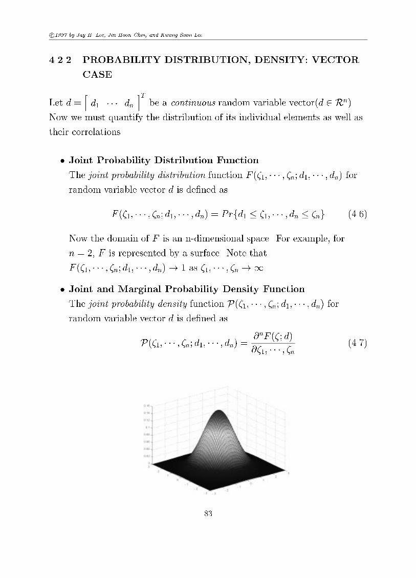
4.2.2 PROBABILITY DISTRIBUTION, DENSITY: VECTOR

CASE

Let d =�d1 � � � dn

�Tbe a continuous random variable vector(d 2 Rn).

Now we must quantify the distribution of its individual elements as well as

their correlations.

� Joint Probability Distribution Function

The joint probability distribution function F (�1; � � � ; �n; d1; � � � ; dn) forrandom variable vector d is de�ned as

F (�1; � � � ; �n; d1; � � � ; dn) = Prfd1 � �1; � � � ; dn � �ng (4.6)

Now the domain of F is an n-dimensional space. For example, for

n = 2, F is represented by a surface. Note that

F (�1; � � � ; �n; d1; � � � ; dn)! 1 as �1; � � � ; �n !1.

� Joint and Marginal Probability Density Function

The joint probability density function P(�1; � � � ; �n; d1; � � � ; dn) forrandom variable vector d is de�ned as

P(�1; � � � ; �n; d1; � � � ; dn) = @nF (�; d)

@�1; � � � ; �n (4.7)

83


For convenience, we may write P(�; d) to denoteP(�1; � � � ; �n; d1; � � � ; dn). Again,

R b1a1� � � R bnan P(�1; � � � ; �n; d1; � � � ; dn) d�1 � � � d�n

= Prfa1 < d1 � b1; � � � ; an < dn � bng(4.8)

Naturally,

Z 1�1; � � � ;

Z 1�1P(�1; � � � ; �n; d1; � � � ; dn)d�1 � � � d�n = 1 (4.9)

We can easily derive the probability density of individual element from

the joint probability density. For instance,

P(�1; d1) =Z 1�1; � � � ;

Z 1�1P(�1; � � � ; �n; d1; � � � ; dn) d�2 � � � d�n (4.10)

This is called marginal probability density.

While the joint probability density (or distribution) tells us the

likelihood of several random variables achieving certain values

simultaneously, the marginal density tells us the likelihood of one

element achieving certain value when the others are not known.

Note that in general

P(�1; � � � ; �n; d1; � � � ; dn) 6= P(�1; d1) � � � P(�n; dn) (4.11)

If

P(�1; � � � ; �n; d1; � � � ; dn) = P(�1; d1) � � � P(�n; dn) (4.12)

d1; � � � ; dn are called mutually independent.

Example: Guassian or Jointly Normally Distributed Variables

84


Suppose that d �= [d1 d2]T is a Gaussian variable. The density takes the

form of

P(�1; �2; d1; d2) =1

2��1�2(1� �2)1=2exp

8<:� 1

2(1� �2)

24 �1 �m1

�1

!2

�2�(�1 �m1)(�2 �m2)

�1�2+ �2 �m2

�2

!2359=; (4.13)

Note that this density is determined by �ve parameters (the means m1;m2,

standard deviations �1; �2 and correlation parameter �). � = 1 represents

complete correlation between d1 and d2, while � = 0 represents no

correlation.

It is fairly straightforward to verify that

P(�1; d1) =Z 1�1P(�1; �2; d1; d2) d�2 (4.14)

=1q2��2

1

exp

8<:�1

2

�1 �m1

�1

!29=; (4.15)

P(�2; d2) =Z 1�1P(�1; �2; d1; d2) d�1 (4.16)

=1q2��2

2

exp

8<:�1

2

�2 �m2

�2

!29=; (4.17)

Hence, (m1; �1) and (m2; �2) represent parameters for the marginal density

of d1 and d2 respectively. Note also that

P(�1; �2; d1; d2) 6= P(�1; d1)P(�2; d2) (4.18)

85


except when � = 0.

General n-dimensional Gaussian random variable vector d = [d1; � � � ; dn]Thas the density function of the following form:

P(�; d) �= P(�1; � � � ; �n; d1; � � � ; dn) (4.19)

=1

(2�)n2 jPdj1=2 exp

(�1

2(� � �d)TP�1

d (� � �d))

(4.20)

where the parameters are �d 2 Rn and Pd 2 Rn�n. The signi�cance of theseparameters will be discussed later.

4.2.3 EXPECTATION OF RANDOM VARIABLES AND

RANDOM VARIABLE FUNCTIONS: SCALAR CASE

Random variables are completely characterized by their distribution

functions or density functions. However, in general, these functions are

nonparametric. Hence, random variables are often characterized by their

moments up to a �nite order; in particular, use of the �rst two moments is

quite common.

� Expection of Random Variable Fnction

Any function of d is a random variable. Its expectation is computed as

follows:

Eff(d)g �=Z 1�1 f(�)P(�; d) d� (4.21)

� Mean

�d �= Efdg =Z 1�1 �P(�; d) d� (4.22)

The above is called mean or expectation of d.

� Variance

86


Varfdg �= Ef(d� �d)2g =Z 1�1(� � �d)2P(�; d) d� (4.23)

The above is the \variance" of d and quanti�es the extent of d

deviating from its mean.

Example: Gaussian Variable

For Gaussian variable with density

P(�; d) = 1p2��2

exp

8<:�1

2

� �m

�

!29=; (4.24)

it is easy to verify that

�d �= Efdg =Z 1�1 �

1p2��2

exp

8<:�1

2

� �m

�

!29=; d� = m (4.25)

Varfdg �= Ef(d� �d)2g =Z 1�1(� �m)2

1p2��2

exp

8<:�1

2

� �m

�

!29=; d� = �2

(4.26)

Hence, m and �2 that parametrize the normal density represent the mean

and the variance of the Gaussian variable.

4.2.4 EXPECTATION OF RANDOM VARIABLES AND

RANDOM VARIABLE FUNCTIONS: VECTOR CASE

We can extend the concepts of mean and variance similarly to the vector

case. Let d be a random variable vector that belongs to Rn.

�d` = Efd`g =Z 1�1 �`P(�`; d`) d�` (4.27)

=Z 1�1 � � �

Z 1�1 �`P(�1; � � � ; �n; d1; � � � ; dn) d�1; � � � ; d�n

Varfd`g = Ef(d` � �d`)2g =

Z 1�1(�` � �d`)

2P(�`; d`) d�` (4.28)

87


=Z 1�1 � � �

Z 1�1(�` � �d`)

2P(�1; � � � ; �n; d1; � � � ; dn) �1; � � � ; d�n

In the vector case, we also need to quantify the correlations among di�erent

elements.

Covfd`; dmg = Ef(d` � �d`)(dm � �dm)g (4.29)

=Z 1�1 � � �

Z 1�1(�` � �d`)(�m � �dm)P(�1; � � � ; �n; d1; � � � ; dn) d�1; � � � ; d�n

Note that

Covfd`; d`g = Varfd`g (4.30)

The ratio

� =Covfd`; dmgq

Varfd`gVarfdmg(4.31)

is the correlation factor. � = 1 indicates complete correlation (d` is

determined uniquely by dm and vice versa). � = 0 indicates no correlation.

It is convenient to de�ne covariance matrix for d, which contains all

variances and covariances of d1; � � � ; dn.

Covfdg = Ef(d� �d)(d� �d)Tg (4.32)

=Z 1�1 � � �

Z 1�1(� � �d)(� � �d)TP(�1; � � � ; �n; d1; � � � ; dn) d�1; � � � ; d�n

The (i; j)th element of Covfdg is Covfdi; djg. The diagonal elements of

Covfdg are variances of elements of d. The above matrix is symmetric since

Covfdi; djg = Covfdj; dig (4.33)

Covariance of two di�erent vectors x 2 Rn and y 2 Rm can be de�ned

similarly.

Covfx; yg = Ef(x� �x)(y � �y)Tg (4.34)

88


In this case, Covfx; yg is an n�m matrix. In addition,

Covfx; yg = (Covfy; xg)T (4.35)

Example: Gaussian Variables { 2-Dimensional Case

Let d = [d1 d2]T and

P(�; d) =1

2��1�2(1� �2)1=2exp

8<:� 1

2(1� �2)

24 �1 �m1

�1

!2(4.36)

�2�(�1 �m1)(�2 �m2)

�1�2+ �2 �m2

�2

!2359=;

Then,

Efdg =Z 1�1

Z 1�1

264 �1�2

375P(�; d) d�1d�2 (4.37)

=

264 m2

m2

375

Similarly, one can show that

Covfdg =Z 1�1

Z 1�1

264 �1 �m1

�2 �m2

375 � (�1 �m1) (�2 �m2)

�P(�; d) d�1d�2

=

264 �2

1 �1�2�

�1�2� �22

375 (4.38)

Example: Gaussian Variables { n-Dimensional Case

Let d = [d1 � � � dn]T and

P(�; d) = 1

(2�)n2 jPdj1=2 exp

(�1

2(� � �d)TP�1

d (� � �d))

(4.39)

89


Then, one can show that

Efdg =Z 1�1 � � �

Z 1�1 �P(�; d) d�1; � � � ; d�n = �d (4.40)

Covfdg =Z 1�1 � � �

Z 1�1(� � �d)(� � �d)TP(�; d) d�1; � � � ; d�n = Pd(4.41)

Hence, �d and Pd that parametrize the normal density function P(�; d)represent the mean and the covariance matrix.

Exercise: Verify that, with

�d =

264 m1

m2

375 ; Pd =

264 �2

1 �1�2�

�1�2� �22

375 (4.42)

one obtains the expression for normal density of a 2-dimensional vector

shown earlier.

NOTE: Use of SVD for Visualization of Normal Density

Covariance matrix Pd contains information about the spread (i.e., extent of

deviation from the mean) for each element and their correlations. For

instance,

Varfd`g = [Covfdg]`;` (4.43)

�fd`; dmg =[Covfdg]`;mq

[Covfdg]`;` [Covfdg]m;m

(4.44)

where [�]i;j represents the (i; j)th element of the matrix. However, one still

has hard time understanding the correlations among all the elements and

visualizing the overall shape of the density function. Here, the SVD can be

useful. Because Pd is a symmetric matrix, it has the following SVD:

Pd�= Ef(d� �d)(d� �d)Tg (4.45)

= V �V T (4.46)

90


=�v1 � � � vn

�2666664�1

. . .

�n

3777775

2666664vT1...

vTn

3777775 (4.47)

Pre-multiplying V T and post-multiplying V to both sides, we obtain

EfV T (d� �d)(d� �d)TV g =

2666664�1

. . .

�n

3777775 (4.48)

Let d� = V Td. Hence, d� is the representation of d in terms of the coordinate

system de�ned by orthonormal basis v1; � � � ; vn. Then, we see that

Ef(d� � �d�)(d� � �d�)Tg =

2666664�1

. . .

�n

3777775 (4.49)

The diagonal covariance matrix means that every element of d� iscompletely independent of each other. Hence, v1; � � � ; vn de�ne the coordiatesystem with respect to which the random variable vector is independent.

�21; � � � ; �2

n are the variances of d� with respect to axes de�ned by v1; � � � ; vn.

Exercise: Suppose d 2 R2 is zero-mean Gaussian and

Pd =

264 20:2 19:8

19:8 20:2

375 =

264p22

p22p

22

�p22

375264 10 0

0 0:1

375264p22

p22p

22

�p22

375 (4.50)

Then, v1 = [p22

p22]T and v2 = [

p22�

p22]T . Can you visualize the overall

shape of the density function? What is the variance of d along the (1,1)

direction? What about along the (1,-1) direction? What do you think the

conditional density of d1 given d2 = � looks like? Plot the densities to verify.

91


4.2.5 CONDITIONAL PROBABILITY DENSITY: SCALAR

CASE

When two random variables are related, the probability density of a random

variable changes when the other random variable takes on a particular value.

The probability density of a random variable when one or more

other random variables are �xed is called conditional probability

density.

This concept is important in stochastic estimation as it can be used to

develop estimates of unknown variables based on readings of other related

variables.

Let x and y be random variables. Suppose xand y have joint probability

density P(�; �;x; y). One may then ask what the probability density of x is

given a particular value of y (say y = �). Formally, this is called

\conditional density function" of x given y and denoted as P(�j�;xjy).P(�j�;xjy) is computed as

P(�j�;xjy) =lim�!0

R �+�� P(�; ��;x; y)d��Z 1

�1

Z �+�

�� P(�; ��;x; y)d��d�| {z }

normalization factor

(4.51)

=P(�; �;x; y)R1

�1P(�; �;x; y)d�(4.52)

=P(�; �;x; y)P(�; y) (4.53)

92


Note:

� The above means0B@ Conditional Density

of x given y

1CA =

Joint Density of x and y

Marginal Density of y(4.54)

This should be quite intuitive.

� Due to the normalization,

Z 1�1P(�j�;xjy) d� = 1 (4.55)

which is what we want for a density function.

�P(�j�;xjy) = P(�; x) (4.56)

if and only if

P(�; �;x; y) = P(�; x)P(�; y) (4.57)

This means that the conditional density is same as the marginal

density when and only when x and y are independent.

We are interested in the conditional density, because often some of the

random variables are measured while others are not. For a particular trial,

if x is not measurable, but y is, we are intersted in knowing P(�j�;xjy) forestimation of x.

Finally, note the distinctions among di�erent density functions:

93


� P(�; �;x; y): Joint Probability Density of x and y

represents the probability density of x = � and y = � simultaneously.

Z b2

a2

Z b1

a1P(�; �;x; y)d�d� = Prfa1 < x � b1 and a2 < y � b2g (4.58)

� P(�;x): Marginal Probability Density of x

represents the probability density of x = � NOT knowing what y is.

P(�; x) =Z 1�1P(�; �;x; y)d� (4.59)

� P(�; y): Marginal Probability Density of y

represents the probability density of y = � NOT knowing what x is.

P(�; y) =Z 1�1P(�; �;x; y)d� (4.60)

� P(�j�;xjy): Conditional Probability Density of x given y

represents the probability density of x when y = �.

P(�j�;xjy) = P(�; �;x; y)P(�; y) (4.61)

� P(�j�; yjx): Conditional Probability Density of y given x

represents the probability density of y when x = �.

P(�j�; yjx) = P(�; �;x; y)P(�; x) (4.62)

Baye's Rule:

Note that

P(�j�;xjy) =P(�; �;x; y)P(�; y) (4.63)

P(�j�; yjx) =P(�; �;x; y)P(�; x) (4.64)

94


Hence, we arrive at

P(�j�;xjy) = P(�j�; yjx)P(�; x)P(�; y) (4.65)

The above is known as the Baye's Rule. It essentially says

(Cond. Prob. of x given y) � (Marg. Prob. of y) (4.66)

= (Cond. Prob. of y given x)� (Marg. Prob. of x) (4.67)

Baye's Rule is useful, since in many cases, we are trying to compute

P(�j�;xjy) and it's di�cult to obtain the expression for it directly, while it

may be easy to write down the expression for P(�j�; yjx).

We can de�ne the concepts of conditional expectation and conditional

covariance using the conditional density. For instance, the conditional

expectation of x given y = � is de�ned as

Efxjyg �=Z 1�1 �P(�j�;xjy)d� (4.68)

Conditional variance can be de�ned as

Varfxjyg �= Ef(� �Efxjyg)2g (4.69)

=Z 1�1(� � Efxjyg)2P(�j�;xjy)d� (4.70)

Example: Jointly Normally Distributed or Gaussian Variables

Suppose that x and y have the following joint normal densities

parametrized by m1;m2; �1; �2; �:

P(�; �;x; y) =1

2��x�y(1� �2)1=2(4.71)

� exp

8><>:�

1

2(1� �2)

264 � � �x

�x

!2� 2�

(� � �x)(� � �y)

�x�y+

0@� � �y

�y

1A23759>=>;

95


Some algebra yields

P(�; �;x; y) =1q2��2

y

exp

8><>:�

1

2

0@� � �y

�y

1A29>=>;| {z }

marginal density of y

(4.72)

� 1q2��2

x(1� �2)exp

8>><>>:�

1

2

0B@� � �x� ��x�y (� � �y)

�xp1� �2

1CA29>>=>>;| {z }

conditional density of x

=1q2��2

x

exp

8<:�1

2

� � �x

�x

!29=;| {z }

marginal density of x

(4.73)

� 1q2��2

y(1� �2)exp

8><>:�

1

2

0@� � �y � ��y�x (� � �x)

�yp1� �2

1A29>=>;| {z }

conditional density of y

Hence,

P(�j�;xjy) =1q

2��2x(1� �2)

exp

8>><>>:�

1

2

0B@� � �x� ��x�y (� � �y)

�xp1� �2

1CA29>>=>>;(4.74)

P(�j�; yjx) =1q

2��2y(1� �2)

exp

8><>:�

1

2

0@� � �y � ��y�x (� � �x)

�yp1� �2

1A29>=>;(4.75)

Note that the above conditional densities are normal. For instance,

P(�j�;xjy) is a normal density with mean of �x+ ��x�y (� � �y) and variance of

�2x(1� �2). So,

Efxjyg = �x+ ��x�y(� � �y) (4.76)

= �x+��x�y�2y

(� � �y) (4.77)

= Efxg+ Covfx; ygVar�1fyg(� � �y) (4.78)

96


Conditional covariance of x given y = � is:

Ef(x�Efxjyg)2jyg = �2x(1� �2) (4.79)

= �2x �

�2x�

2y�

2

�2y

(4.80)

= �2x � (�x�y�)

1

�2y

(�x�y�) (4.81)

= Varfxg � Covfx; ygVar�1fygCovfy; xg(4.82)

Notice that the conditional distribution becomes a point density as �! 1,

which should be intuitively obvious.

4.2.6 CONDITIONAL PROBABILITY DENSITY: VECTOR

CASE

We can extend the concept of conditional probability distribution to the

vector case similarly as before.

Let x and y be n and m dimensional random vectors respectively. Then, the

conditional density of x given y = [�1; � � � ; �m]T is de�ned as

P(�1; � � � ; �nj�1; � � � ; �m;x1; � � � ; xnjy1; � � � ; ym)=

P(�1; � � � ; �n; �1; � � � ; �m;x1; � � � ; xn; y1; � � � ; ym)P(�1; � � � ; �m; y1; � � � ; ym) (4.83)

Baye's Rule can be stated as

P(�1; � � � ; �nj�1; � � � ; �m;x1; � � � ; xnjy1; � � � ; ym) (4.84)

=P(�1; � � � ; �mj�1; � � � ; �n; y1; � � � ; ymjx1; � � � ; xn)P(�1; � � � ; �n;x1; � � � ; xn)

P(�1; � � � ; �m; y1; � � � ; ym)

97


The conditional expectation and covariance matrix can be de�ned similarly:

Efxjyg =Z 1�1 � � �

Z 1�1

2666664�1...

�n

3777775P(�j�;xjy) d�1; � � � ; d�n (4.85)

Covfxjyg =Z 1�1 � � �

Z 1�1

2666664�1 �Efx1jyg

...

�n �Efxnjyg

3777775

2666664�1 � Efx1jyg

...

�n � Efxnjyg

3777775

T

P(�j�;xjy) d�1; � � � ; d�n

(4.86)

Example: Gaussian or Jointly Normally Distributed Variables

Let x and y be jointly normally distributed random variable vectors of

dimension n and m respectively. Let

z =

264 xy

375 (4.87)

The joint distribution takes the form of

P(�; �;x; y) = 1

(2�)n+m2 jPzj1=2

exp(�1

2(� � �z)TP�1

z (� � �z))

(4.88)

where

�z =

264 �x

�y

375 ; � =

264 �

�

375 (4.89)

Pz =

264 Cov(x) Cov(x; y)

Cov(y; x) Cov(y)

375 (4.90)

Then, it can be proven that (see Theorem 2.13 in [Jaz70])

Efxjyg = �x+Cov(x; y)Cov�1(y)(� � �y) (4.91)

Efyjxg = �y + Cov(y; x)Cov�1(x)(� � �x) (4.92)

98


and

Covfxjyg �= E�(� �Efxjyg) (� � Efxjyg)T

�(4.93)

= Covfxg � Covfx; ygCov�1fygCovfy; xg (4.94)

Covfyjxg �= E�(� � Efyjxg) (� � Efyjxg)T

�(4.95)

= Covfyg � Covfy; xgCov�1fxgCovfx; yg (4.96)

4.3 STATISTICS

4.3.1 PREDICTION

The �rst problem of statistics is prediction of the outcome of a future trial

given a probabilistic model.

Suppose P(x), the probability density for random variable x, is

given. Predict the outcome of x for a new trial (which is about to

occur).

Note that, unless P(x) is a point distribution, x cannot be predicted exactly.

To do optimal estimation, one must �rst establish a formal criterion. For

example, the most likely value of x is the one that corresponds to the

highest density value:

x = arg�maxxP(x)

�

A more commonly used criterion is the following minimum variance

estimate:

x = arg�minx

Enkx� xk22

o�

The solution to the above is x = Efxg.Exercise: Can you prove the above?

99


If a related variable y (from the same trial) is given, then one should use

x = Efxjyg instead.

4.3.2 SAMPLE MEAN AND COVARIANCE,

PROBABILISTIC MODEL

The other problem of statistics is inferring a probabilistic model from

collected data. The simplest of such problems is the following:

We are given the data for random variable x from N trials. These

data are labeled as x(1); � � � ; x(N). Find the probability density

function for x.

Often times, a certain density shape (like normal distribution) is assumed to

make it a well-posed problem. If a normal density is assumed, the following

sample averages can then be used as estimates for the mean and covariance:

�x =1

N

NXi=1

x(i)

Rx =1

N

NXi=1

x(i)xT(i)

Note that the above estimates are consistent estimates of real mean and

covariance �x and Rx (i.e., they converge to true values as N !1).

A slightly more general problem is:

A random variable vector y is produced according to

y = f(�; u) + x

In the above, x is another random variable vector, u is a known

deterministic vector (which can change from trial to trial) and � is

100


an unknown deterministic vector (which is invariant). Given data

for y from N trials, �nd the probability density parameters for x

(e.g., �x, Rx) and the unknown deterministic vector �.

This problem will be discussed later in the regression section.

101


Chapter 5

STOCHASTIC PROCESSES

A stochastic process refers to a family of random variables indexed by a

parameter set. This parameter set can be continuous or discrete. Since we

are interested in discrete systems, we will limit our discussion to processes

with a discrete parameter set. Hence, a stochastic process in our context is

a time sequence of random variables.

5.1 BASIC PROBABILITY CONCEPTS

5.1.1 DISTRIBUTION FUNCTION

Let x(k) be a sequence. Then, (x(k1); � � � ; x(k`)) form an `-dimensional

random variable. Then, one can de�ne the �nite dimensional distribution

function and the density function as before. For instance, the distribution

function F (�1; � � � ; �`;x(k1); � � � ; x(k`)), is de�ned as:

F (�1; � � � ; �`;x(k1); � � � ; x(k`)) = Prfx(k1) � �1; � � � ; x(k`) � �`g (5.1)

The density function is also de�ned similarly as before.

We note that the above de�nitions also apply to vector time sequences if

102


x(ki) and �i's are taken as vectors and each integral is de�ned over the

space that �i occupies.

5.1.2 MEAN AND COVARIANCE

Mean value of the stochastic variable x(k) is

�x(k) = Efx(k)g =Z 1�1 �dF (�;x(k)) (5.2)

Its covariance is de�ned as

Rx(k1; k2) = Ef[x(k1)� �x(k1)][x(k2)� �x(k2)]Tg

=R1�1

R1�1[�1 � �x(k1)][�2 � �x(k2)]

TdF (�1; �2;x(k1); x(k2))

(5.3)

The cross-covariance of two stochastic processes x(k) and y(k) are de�ned as

Rxy(k1; k2) = Ef[x(k1)� �x(k1)][y(k2)� �y(k2)]Tg

=R1�1

R1�1[�1 � �x(k1)][�2 � �y(k2)]

TdF (�1; �2;x(k1); y(k2))

(5.4)

Gaussian processes refer to the processes of which any �nite-dimensional

distribution function is normal. Gaussian processes are completely

characterized by the mean and covariance.

5.1.3 STATIONARY STOCHASTIC PROCESSES

Throughout this book we will de�ne stationary stochastic processes as those

with time-invariant distribution function. Weakly stationary (or stationary

in a wide sense) processes are processes whose �rst two moments are

103


time-invariant. Hence, for a weakly stationary process x(k),

Efx(k)g = �x 8kEf[x(k)� �x][x(k � �)� �x]Tg = Rx(�) 8k (5.5)

In other words, if x(k) is stationary, it has a constant mean value and its

covariance depends only on the time di�erence � . For Gaussian processes,

weakly stationary processes are also stationary.

For scalar x(k), R(0) can be interpreted as the variance of the signal andR(�)R(0) reveals its time correlation. The normalized covariance R(�)

R(0) ranges from

0 to 1 and indicates the time correlation of the signal. The value of 1

indicates a complete correlation and the value of 0 indicates no correlation.

Note that many signals have both deterministic and stochastic components.

In some applications, it is very useful to treat these signals in the same

framework. One can do this by de�ning

�x = limN!1 1N

PNk=1 x(k)

Rx(�) = limN!1 1N

PNk=1[x(k)� �x][x(k � �)� �x]T

(5.6)

Note that in the above, both deterministic and stochastic parts are

averaged out. The signals for which the above limits converge are called

\quasi-stationary" signals. The above de�nitions are consistent with the

previous de�nitions since,in the purely stochastic case, a particular

realization of a stationary stochastic process with given mean (�x) and

covariance (Rx(�)) should satisfy the above relationships.

5.1.4 SPECTRA OF STATIONARY STOCHASTIC

PROCESSES

Throughout this chapter, continuous time is rescaled so that each discrete

time interval represents one continuous time unit. If the sample interval Ts

104


is not one continuous time unit, the frequency in discrete time needs to be

scaled with the factor of 1Ts.

Spectral density of a stationary process x(k) is de�ned as the Fourier

transform of its covariance function:

�x(!) =1

2�

1X�=�1

Rx(�)e�j�! (5.7)

Area under the curve represents the power of the signal for the particular

frequency range. For example, the power of x(k) in the frequency range

(!1; !2) is calculated by the integral

2 �Z !=!2

!=!1�x(!)d!

Peaks in the signal spectrum indicate the presence of periodic components

in the signal at the respective frequency.

The inverse Fourier transform can be used to calculate Rx(�) from the

spectrum �x(!) as well

Rx(�) =Z �

�� x(!)ej�!d! (5.8)

With � = 0, the above becomes

Efx(k)x(k)Tg = Rx(0) =Z �

�� x(!)d! (5.9)

which indicates that the total area under the spectral density is equal to the

variance of the signal. This is known as the Parseval's relationship.

Example: Show plots of various covariances, spectra and realizations!

**Exercise: Plot the spectra of (1) white noise, (2) sinusoids, and (3)white

noise �ltered through a low-pass �lter.

105


5.1.5 DISCRETE-TIME WHITE NOISE

A particular type of a stochastic process called white noise will be used

extensively throughout this book. x(k) is called a white noise (or white

sequence) if

P(x(k)jx(`)) = P(x(k)) for ` < k (5.10)

for all k. In other words, the sequence has no time correlation and hence all

the elements are mutually independent. In such a situation, knowing the

realization of x(`) in no way helps in estimating x(k).

A stationary white noise sequence has the following properties:

Efx(k)g = �x 8k

Ef(x(k)� �x)(x(k � �)� �x)Tg =

8><>:Rx if � = 0

0 if � 6= 0

(5.11)

Hence, the covariance of a white noise is de�ned by a single matrix.

The spectrum of white noise x(k) is constant for the entire frequency range

since from (5.7)

�x(!) =1

2�Rx (5.12)

The name \white noise" actually originated from its similarity with white

light in spectral properties.

5.1.6 COLORED NOISE

A stochastic process generated by �ltering white noise through a dynamic

system is called \colored noise."

Important:

106


A stationary stochastic process with any given mean and

covariance function can be generated by passing a white noise

through an appropriate dynamical system.

To see this, consider

d(k) = H(q)"(k) + �d (5.13)

where "(k) is a white noise of identity covariance and H(q) is a stable /

stably invertible transfer function (matrix). Using simple algebra (Ljung

-REFERENCE), one can show that

�d(!) = H(ej!)HT (e�j!) (5.14)

The spectral factorization theorem (REFERENCE - �Astr�om and

Wittenmark, 1984) says that one can always �nd H(q) that satis�es (5.14)

for an arbitrary �d and has no pole or zero outside the unit disk. In other

words, the �rst and second order moments of any stationary signal can be

matched by the above model.

This result is very useful in modeling disturbances whose covariance

functions are known or �xed. Note that a stationary Gaussian process is

completely speci�ed by its mean and covariance. Such a process can be

modelled by �ltering a zero-mean Gaussian white sequence through

appropriate dynamics determined by its spectrum (plus adding a bias at the

output if the mean is not zero).

107


5.1.7 INTEGRATED WHITE NOISE AND

NONSTATIONARY PROCESSES

Some processes exhibit mean-shifts (whose magnitude and occurence are

random). Consider the following model:

y(k) = y(k � 1) + "(k)

where "(k) is a white sequence. Such a sequence is called integrated white

noise or sometimes random walk. Particular realizations under di�erent

distribution of "(k) are shown below:

P(ζ )

��90%

10%

y(k)

More generally, many interesting signals will exhibit stationary behavior

combined with randomly occuring mean-shifts. Such signals can be modeled

as

108


~( )H q 1−

1

1 q 1− − H q 1( )−

1

1 q 1− −

ε2(k )

ε1(k )

ε(k )

+ +

y(k)

y(k)

As shown above, the combined e�ects can be expressed as an integrated

white noise colored with a �lter H(q�1).

Note that while y(k) is nonstationary, the di�erenced signal �y(k) is

stationary.

y(k)1

1 q 1− −

ε(k )H q 1( )− H q 1( )−ε(k ) ∆y(k)

5.1.8 STOCHASTIC DIFFERENCE EQUATION

Generally, a stochastic process can be modeled through the following

stochastic di�erence equation.

x(k + 1) = Ax(k) +B"(k)

y(k) = Cx(k) +D"(k)(5.15)

where "(k) is a white vector sequence of zero mean and covariance R".

Note that

Efx(k)g = AEfx(k � 1)g = AkEfx(0)gEfx(k)xT(k)g = AEfx(k � 1)xT(k � 1)gAT + BR"B

T(5.16)

109


If all the eigenvalues of A are strictly inside the unit disk, the above

approaches a stationary process as k !1 since

limk!1Efx(k)g = 0

limk!1Efx(k)xT(k)g = Rx

(5.17)

where Rx is a solution to the Lyapunov equation

Rx = ARxAT +BR"B

T (5.18)

Since y(k) = Cx(k) +D"(k),

Efy(k)g = CEfx(k)g+DEf"(k)g = 0

Efy(k)yT (k)g = CEfx(k)xT(k)gCT +DEf"(k)"T (k)gDT = CRxCT +DR"D

T

(5.19)

The auto-correlation function of y(k) becomes

Ry(�)�= Efy(k + �)yT (k)g =

8><>:CRxC

T +DR"DT for � = 0

CA�RxCT + CA��1BR"D

T for � > 0(5.20)

The spectrum of w is obtained by taking the Fourier transform of Ry(�))

and can be shown to be

�y(!) =�C(ej!I � A)�1B +D

�R"

�C(ej!I � A)�1B +D

�T(5.21)

In the case that A contains eigenvalues on or outside the unit circle, the

process is nonstationary as its covariance keeps increasing (see Eqn. (5.16).

However, it is common to include integrators in A to model mean-shifting

(random-walk-like) behavior. If all the outputs exhibit this behavior, one

can usex(k + 1) = Ax(k) +B"(k)

�y(k) = Cx(k) +D"(k)(5.22)

Note that, with a stable A, while �y(k) is a stationary process, y(k)

110


includes an integrator and therefore is nonstationary.

ε(κ) ε(κ)y(k) ∆y(k) y(k)

stable system stable system integrator

Stationary process Nonstationary(Meanshifting) process

x(k+1)=Ax(k)+B ε(k)y(k)=Cx(k)+D ε(k)

x(k+1)=Ax(k)+B ε(k)y(k)=Cx(k)+D ε(k)

1-q -1

1

5.2 STOCHASTIC SYSTEM MODELS

Models used for control will often include both deterministic and stochastic

inputs. The deterministic inputs correspond to known signals like

manipulated variables. The stochastic signals cover whatever remaining

parts that cannot be predicted a priori. They include the e�ect of

disturbances, other process variations and instrumentation errors.

5.2.1 STATE-SPACE MODEL

The following stochastic di�erence equation may be used to characterize a

stochastic disturbance:

x(k + 1) = Ax(k) +Bu(k) + "1(k)

y(k) = Cx(k) + "2(k)(5.23)

"1(k) and "2(k) are white noise sequences that represent the e�ects of

disturbances, measurement error, etc. They may or may not be correlated.

� If the above model is derived from fundamental principles, "(k) may be

a signal used to generate physical disturbance states (which are

111


included in the state x) or merely arti�cal signals added to represent

random errors in the state equation. "2(k) may be measurement noise

or signals representing errors in the output equations.

� If the model is derived on an empirical basis, "1(k) and "2(k) together

represent the combined e�ects of the process / measurement

randomness. In other words, the output is viewed as a composite of

two signals (y(k) = yd(k) + ys(k)), one of which is the output of the

deterministic system

x(k + 1) = Ax(k) + Bu(k)

yd(k) = Cx(k)(5.24)

and the other is the random component

x(k + 1) = Ax(k) + "1(k)

ys(k) = Cx(k) + "2(k)(5.25)

With such a model available, one problem treated in statistics is to predict

future states, (x(k + i); i � 0) given collected output measurements

(y(k); � � � ; y(1)). This is called state estimation and will be discussed in the

next chapter.

The other problem is building such a model. Given data

(y(i); u(i); i = 1; � � � ; N), the following two methods are available.

� One can use the so called subspace identi�cation methods.

� One can build a time series model or more generally a transfer function

model of the form

y(k) = G(q�1)u(k) +H(q�1)"(k)

Then, one can perform a state-space realization of the above to obtain

the state-space model.

112


Details of these methods will be discussed in the identi�cation chapter.

For systems with (mean-shifting) nonstationary disturbances in all output

channels, it may be more convenient to express the model in terms of the

di�erenced inputs and outputs:

x(k + 1) = Ax(k) + B�u(k) + "1(k)

�y(k) = Cx(k) + "2(k)(5.26)

If the undi�erenced y is desired as the output of the system, one can simply

rewrite the above as264 x(k + 1)

y(k + 1)

375 =

264 A 0

CA I

375264 x(k)y(k)

375+

264 B

CB

375�u(k) +

264 I

C

375 "1(k) +

264 0

I

375 "2(k)

y(k) =�0 I

� 264 x(k)y(k)

375

(5.27)

113


Nonlinear ODE'szf = f(z f,u f,w f)

y f = f(z f)

I/O Datau(1), ,u(N)

y(1), ,y(N)

Physio-ChemicalPrinciples

I/D ExperimentHistorical Data Base

x(k+1) = Ax(k) + Bu(k) + ε1(k)

y(k) = Cx(k) + ε2(k)

Linear Difference Eqns:

z(k+1)=Az(k)+B uu(k)+B ww(k)

y(k)=Cz(k)

Discrete Transfer Functions

y(k)=G(q -1,θ)u(k)+H(q -1,θ )e(k)

Augmentation StochasticStates

z

wx

Realization

ParametericID(PEM)

Linearization+

Discretization

Subspace I D

5.2.2 INPUT-OUTPUT MODELS

One can also use input-output models. A general form is

y(k) = G(q)u(k) +H(q)"(k) (5.28)

114


Within the above general structure, di�erent parameterizations exist. For

instance, a popular model is the following ARMAX (AR for

Auto-Regressive, MA for Moving-Average and X for eXtra input) process:

y(k) = (I + A1q�1 + � � �+Anq

�n)�1(B1q�1 + � � �+ Bmq

�m)u(k)+(I + A1q

�1 + � � �+Anq�n)�1(I + C1q

�1 + � � �+ Cnq�n)"(k)

(5.29)

Note that the above is equivalent to the following linear time-series

equation:

y(k) = �A1y(k � 1)� A2y(k � 2)� � � � � Any(k � n)

+B1u(k � 1) + � � �+ Bmu(k �m)

+"(k) + C1"(k � 1) + � � �+ Cn"(k � n)

(5.30)

In most practical applications, matrices Ai's and Ci's are restricted to be

diagonal, which results in a MISO (rather than a MIMO) structure. In such

a case, stochastic components for di�erent output channels are restricted to

be mutually independent.

For systems with integrating type disturbances in all output channels, a

more appropriate model form is

y(k) = G(q)u(k) +1

1� q�1H(q)"(k) (5.31)

The above can be easily rewritten as

�y(k) = G(q)�u(k) +H(q)"(k) (5.32)

115


Chapter 6

STATE ESTIMATION

In practice, it is unrealistic to assume that all the disturbances and states

can be measured. In general, one must estimate the states from the

measured input / output sequences. This is called state estimation.

Let us assume the standard state-space system description we developed in

the previous chapter:

x(k + 1) = Ax(k) +Bu(k) + "1(k)

y(k) = Cx(k) + "2(k)(6.1)

"1(k) and "2(k) are mutually independent white noise sequences of

covariances R1 and R2 respectively. The problem of state estimation is to

estimate x(k + i); i � 0, given fy(j); u(j); j � kg (i.e., inputs and outputs

up to the kth sample time). Estimating x(k + i) for i > 0 is called

prediction, while that for i = 0 is called �ltering. Some applications require

x(k + i); i < 0 to be estimated and this is referred to as smoothing.

There are many state estimation techniques, ranging from a simple

open-loop observer to more sophisticated optimal observers like the Kalman

�lter. Since state estimation is an integral part of a model predictive

controller, we examine some popular techniques in this chapter. These

116


techniques are also useful for parameter estimation problems, such as those

arise in system identi�cation discussed in the next chapter.

An extremely important, but often overlooked point is the importance of

correct disturbance modelling. Simply adding white noises into the state

and output equations, as often done by those who misunderstand the role of

white noise in a standard system description, can result in extreme bias. In

general, to obtain satisfactory results, disturbances (or their e�ects) must

be modelled as appropriate stationary / nonstationary stochastic processes

and the system equations must be augmented with their describing

stochastic equations before a state estimation technique is applied.

6.1 LINEAR OBSERVER STRUCTURE

A linear observer for system (6.1) takes the form of

x(kjk � 1) = Ax(k � 1jk � 1) +Bu(k � 1)

x(kjk) = x(kjk � 1) +K(y(k)� x(kjk � 1))(6.2)

In the above, x(ijj) represents an estimate of x(i) constructed using

measurements up to time j. The above equations can be used to construct

the �ltered estimate x(kjk) recursively.

Comments:

� In some applications, one may need to compute the one-step-ahead

prediction x(k + 1jk) rather than the �ltered estimate. For instance, in

a control application, the control computation may require one sample

period to complete and in this case, one may want to compute

x(k + 1jk) at time k in order to begin the computation for the control

input u(k + 1).

117


t=k t=k+1

y(k)

y(k)

u(k+1)

x(k-1|k-1)

u(k-1)

x(k|k-1)

u(k)

x(k|k)

x(k+1|k)

u(k)StateEst.

StateEst.

Controlcomp.

Control Computation

Notice that (6.2) can be rewritten as a one-step-ahead predictor simply

by switching the order of the two equations:

x(kjk) = x(kjk � 1) +K(y(k)� x(kjk � 1))

x(k + 1jk) = Ax(kjk) + Bu(k)(6.3)

� The free parameter in the above is K, which is called the observer gain

matrix. What remains to be discussed is how to choose K. In general,

it should be chosen so that the estimation error (xe(k)�= x(k)� x(kjk)

or xe(k + 1) �= x(k + 1)� x(k + 1jk)) is minimized in some sense.

� Equations for error dynamics can be easily derived. For instance, the

equations for the �lter estimation error is

xe(k) = (A�KCA)xe(k � 1) + (I �KC)"1(k � 1) +K"2(k) (6.4)

118


The above can be derived straightforwardly by replacing y(k) in the

observer equation (6.2) with CAx(k � 1) + CBu(k � 1) + C"1(k � 1).

The equation for prediction error xe(k) can be derived similarly as

xe(k + 1) = (A� AKC)xe(k) + "1(k � 1) +AK"2(k) (6.5)

� In some cases, it is advantageous to allow K to vary with time. This

results in a time varying observer.

6.2 POLE PLACEMENT

From (6.4), it is clear that the eigenvalues of the transition matrix A�KCA

determine how the estimation error propagates. For instance, one must take

care that all the eigenvalues lie strictly inside the unit circle in order to

ensure stable error dynamics (i.e., asymptotically vanishing initialization

error, �nite error variance, etc.). The eigenvalues of A�KCA are called

observer poles and determining K on the basis of prespeci�ed observer pole

location is called pole placement. For instance, if (C;A) is an observable

pair, the observer poles can be placed in an arbitrary manner through K.

One can also work with the one-step-ahead prediction error equation (6.5).

In this case one can let AK = K and determine K so that the eigenvalues

of A� KC are placed at desired locations. Again, with an observer system,

the eigenvalues can be placed at arbitrary locations.

Pole placement is most coveniently carried out by �rst putting the system

in an observer canonical form through an appropriate coordinate

transformation (given by the observability matrix). For instance, consider

the following observer canonical form for a single-input, single-output

119


system:

x(k + 1) =

26666666666664

�a1 1 0 � � � 0

�a2 0 1 � � � 0...

... . . . . . . ...

�an�1 0 0 � � � 1

�an 0 0 � � � 0

37777777777775x(k) +

26666666666664

b1

b2...

bn�1bn

37777777777775u(k)

y(k) =�1 0 � � � 0 0

�x(k)

(6.6)

Then, assuming K = [k1 k2 � � � kn�1 kn]T , we have

A�KC =

26666666666664

�(a1 + k1) 1 0 � � � 0

�(a2 + k2) 0 1 � � � 0...

... . . . . . . ...

�(an�1 + kn�1) 0 0 � � � 1

�(an + kn) 0 0 � � � 0

37777777777775

(6.7)

The characteristic polynomial for the above matrix is

zn + (a1 + k1)zn�1 + � � �+ (an�1 + kn�1)z + (an + kn) = 0 (6.8)

Hence, k1; � � � ; kn can be easily determined to place the roots at desired

locations.

6.3 KALMAN FILTER

An observer gain can also be determined from a stochastic optimal

estimation viewpoint. For example, the observer gain for the linear observer

structure can be chosen to minimize the variance of the estimation error.

The resulting estimator is the celebrated Kalman �lter, which has by far

been the most popular state estimation technique. When the additional

assumption is made that the disturbances are Gaussian, the Kalman �lter is

120


indeed the optimal estimator (not just the optimal linear estimator).

6.3.1 KALMAN FILTER AS THE OPTIMAL LINEAR

OBSERVER

Note that the the linear observer (6.3) can be written in the following

one-step-ahead predictor form:

x(k + 1jk) = Ax(kjk � 1) + Bu(k) +AK(k)| {z }K(k)

fy(k)� Cx(kjk � 1)g (6.9)

In the above, we allowed the observer gain to vary with time for generality.

Recall that the error dynamics for xe(k) = x(k)� x(kjk � 1) are given by

xe(k + 1) = (A� K(k)C)xe(k) + "1(k) + K(k)"2(k) (6.10)

Let

P (k) = Covfxe(k)g (6.11)

= E�(xe(k)�Efxe(k)g) (xe(k)� Efxe(k)g)T

�(6.12)

Assuming that the initial guess is chosen so that Efxe(0)g = 0,

Efxe(k)g = 0 for all k � 0 and

P (k + 1) =nxe(k + 1)xTe (k + 1)

o(6.13)

= (A� K(k)C)P (k)(A� K(k)C)T + R1 � K(k)R2KT (k)

In the above, we used the fact that xe(k); "1(k) and "2(k) in (6.10) are

mutually independent.

Now let us choose K(k) such that �TP (k+1)� is minimized for an arbitrary

choice of �. Since � is an arbitrary vector, this choice of K(k) minimizes

121


the expected value of any norm of xe (including the 2-norm which represents

the error variance). Now, it is straightforward algebra to show that

�TP (k + 1)� = �T�AP (k)AT + R1 � K(k)CP (k)AT (6.14)

�AP (k)CTKT (k) + K(k)(R2 + CP (k)CT )KT (k)��

Completing the square on the terms involving K(k), we obtain

�TP (k + 1)� = �T��K(k)� AP (k)CT (R2 + CP (k)CT )�1

� hR2 + CP (k)CT

i

��K(k)�AP (k)CT (R2 + CP (k)CT )�1

�T)� (6.15)

+�ThAP (k)AT +R1 �AP (k)CT (R2 + CP (k)CT )�1CP (k)AT

i�

Hence, K(k) minimizing the above is

K(k) = AP (k)CT (R2 + CP (k)CT)�1 (6.16)

and

P (k+1) = AP (k)AT +R1�AP (k)CT�R2 + CP (k)CT

��1CP (k)AT (6.17)

Given x(1j0) and P (1), the above equations can be used along with (6.9) to

recursively compute x(k + 1jk). They are referred to as the time-varying

Kalman �lter equations.

Note:

� For detectable systems, it can be shown that P (k) converges to a

constant matrix �P as K !1. Hence, for linear time-invariant

systems, it is customary to implement an observer with a constant gain

matrix derived from �P according to (6.16). This is referred to as the

steady-state Kalman �lter.

122


� Also, recall the relationship between the one-step-ahead predictor gain

K(k) and the �lter gain K(k) (K(k) = AK(k)). Hence,

K(k) = P (k)CT (R2 + CP (k)CT)�1 (6.18)

This gain can be used to implement a �lter of the form (6.2) that

recursively computes x(kjk) rather than x(k + 1jk).

6.3.2 KALMAN FILTER AS THE OPTIMAL ESTIMATOR

FOR GAUSSIAN SYSTEMS

In the previous section, we assumed a linear observer structure and posed

the problem as a parametric optimization where the expected value of the

estimation error variance is minimized with respect to the observer gain. In

fact, the Kalman �lter can be derived from an entirely probabilistic

argument, i.e., by deriving a Bayesian estimator that recursively computes

the conditional density of x(k).

Assume that "1(k) and "2(k) are Gaussian noise sequences. Then, assuming

x(0) is also a Gaussian variable, x(k) and y(k) are jointly-Gaussian

sequences. Now we can simply formulate the state estimation problem as

computing the conditional expectation Efx(k) j Y (k)g whereY (k) = [yT (0); yT (1); � � � ; yT (k)]T . Let us denote Efx(i) j Y (j)g as x(ijj).We divide the estimation into the following two steps.

123


X(k-1|k-1)

P(k-1|k-1)

X(k|k-1)

P(k|k-1)

X(k|k)

P(k|k)

u(k-1)

y(k)

measurementupdate

Modelupdate

� Model Update: Compute Efx(k)jY (k � 1)g givenEfx(k � 1)jY (k � 1)g , P (k � 1jk � 1) , and u(k � 1).

Since x(k) = Ax(k � 1) +Bu(k � 1) + "1(k � 1) and "1(k � 1) is a

zero-mean variable independent of y(0); � � � ; y(k � 1),

x(kjk � 1) = E fAx(k � 1) + Bu(k � 1) + e(k � 1) j Y (k � 1)g= AEfx(k � 1) j Y (k � 1)g+ Bu(k � 1) (6.19)

Hence, we obtain

x(kjk � 1) = Ax(k � 1jk � 1) + Bu(k � 1) (6.20)

In addition, note that

x(k)� x(kjk � 1) = A (x(k)� x(k � 1jk � 1)) + "1(k � 1) (6.21)

Therefore,

P (kjk � 1) = E�(x(k)� x(kjk � 1)) (x(k)� x(kjk � 1))T

�(6.22)

= AP (k � 1jk � 1)AT + R1 (6.23)

Since the conditional density for x(k) given Y (k � 1) is Gaussian, it is

completely speci�ed by x(kjk � 1) and P (kjk � 1).

� Measurement Update: Compute Efx(k)jY (k)g givenEfx(k)jY (k � 1)g P (kjk � 1) and y(k).

124


The conditional density Pfx(k) j Y (k)g is equivalent to the conditionaldensity Pfx(k) j y(k)g with the prior density of x(k) given instead by

Pfx(k) j Y (k � 1)g. Note that Pfx(k) j Y (k � 1)g is a Gaussian

density of mean x(kjk � 1) and covariance P (kjk � 1). In other words,

we view x(k) as a Gaussian variable of mean x(kjk � 1) and covariance

P (kjk � 1).

In addition, y(k) = Cx(k) + "2(k) and therefore is also Gaussian.

Efy(k)g = CEfx(k)g+ Ef"(k)g = Cx(kjk � 1)

E�(y(k)� Efy(k)g) (y(k)� Efy(k)g)T

�= CP (kjk � 1)CT +R2

In fact, x(k) and y(k) are jointly Gaussian with the following

covariance:

E

8>><>>:264 x(k)� x(kjk � 1)

y(k)� y(kjk � 1)

375264 x(k)� x(kjk � 1)

y(k)� y(kjk � 1)

375T9>>=>>;

=

264 P (kjk � 1) P (kjk � 1)CT

CP (kjk � 1) CP (kjk � 1)CT + R2

375

(6.24)

Recall the earlier results for jointly Gaussian variables:

Efxjyg = Efxg+RxyR�1y (y �Efyg) (6.25)

Covfxjyg = Rx �RxyR�1y Ryx (6.26)

Applying the above to x(k) and y(k),

x(kjk) = Efx(k)jy(k)g (6.27)

= x(kjk � 1)

+P (kjk � 1)CT�CP (kjk � 1)CT + R2

��1(y(k)� Cx(kjk � 1))

P (kjk) = Covfx(k)jy(k)g= P (kjk � 1)� P (kjk � 1)CT

�CP (kjk � 1)CT +R2

��1CP (kjk � 1)

125


In short, for Gaussian systems, we can compute the conditional mean and

covariance of x(k) recursively using

x(kjk � 1) = Ax(k � 1jk � 1) +Bu(k � 1)

x(kjk) = x(kjk�1)+P (kjk � 1)CT�CP (kjk � 1)CT + R2

��1| {z }

K(k)

(y(k)�Cx(kjk�1))

and

P (kjk � 1) = AP (k � 1jk � 1)AT + R1

P (kjk) = P (kjk � 1)� P (kjk � 1)CT�CP (kjk � 1)CT +R2

��1CP (kjk � 1)

Note that this above has a linear observer structure with the observer gain

given by the Kalman �lter equations derived earlier (P (kjk � 1) in the

above is P (k) in Eq. (6.16){(6.17)).

126


Chapter 7

SYSTEM IDENTIFICATION

Identi�cation of process dynamics is perhaps the most time consuming step

in implementing an MPC and one that requires relatively high expertise

from the user. In this section, we give introduction to various identi�cation

methods and touch upon some key issues that should help an engineer

obtain models on a reliable basis. Since system identi�cation is a very

broad subject that can easily take up an entire book, we will limit our

objective to giving just an overview and providing a starting point for

further exploration of the �eld. Because of this, our treatment of various

methods and issues will necessarily be brief and informal. References will be

given at the end for more complete, detailed treatments of the various

topics presented in this chapter.

7.1 PROBLEM OVERVIEW

The goal of identi�cation is to obtain a mathematical relation that reliably

predicts the behavior of outputs, using input output data gathered from the

process. For conveninence, the mathematical relation searched for is often

limited to linear ones. As we saw in the previous chapter, both known and

127


unknown inputs a�ect the outputs. Since many inputs change in a random,

but correlated manner, it is often desirable to identify a model that has

both deterministic and stochastic components.

In terms of how input output data are translated into a mathematical

relation, the �eld of identi�cation can be divided broadly into two branches:

parametric identi�cation and nonparametric identi�cation. In parameteric

identi�cation, the structure of the mathematical relation is �xed a priori

and parameters of the structure are �tted to the data. In nonparametric

identi�cation, no (or very little) assumption is made with respect to the

model structure. Frequency response identi�cation is nonparametric.

Impulse response identi�cation is also nonparametric, but it can also be

viewed as parametric identi�cation since a impulse response of a �nite

length is often identi�ed.

As a �nal note, it is important not to forget the end-use of the model,

which is to analyze and design a feedback control system in our case.

Accuracy of a model must ultimately be judged in view of how well the

model predicts the output behavior with the intended feedback control

system in place. This consideration must be re ected in all phases of

identi�cation including test input design, data �ltering, model structure

selection, and parameter estimation.

7.2 PARAMETRIC IDENTIFICATION METHODS

In parametric identi�cation, the model structure is set in prior to the model

�tting. The key objective is then to identify the model parameters, based on

given input output data. Although a particular model structure is assumed

for parameter estimation, one often adjusts the model structure iteratively

based on the result of �tting (for example, through residual analysis).

128


7.2.1 MODEL STRUCTURES

A general structure for parametric identi�cation is:

y(k) = G(q; �)u(k) +H(q; �)"(k) (7.1)

where y is the output and u is the input (most of times, this will be a

manipulated input, but it can also be a measured disturbance variable). For

systems with stationary disturbances, "(k) can be assumed to be white noise

and H(q; �) a stable, stably invertible and normalized (i.e., H(1; �) = 1)

transfer function, without loss of generality. In the case that the

disturbance is better described by a stochastic process driven by integrated

white noise, we can replace y(k) and u(k) with �y(k) and �u(k) .

Within the general structure, di�erent parametrizations exist. Let us

discuss some popular ones, �rst in the single input, single output context.

� ARX Model If we represent G as a rational function and express it

as a linear equation with an additive error term, we obtain

y(k)+a1y(k�1)+ � � �+any(k�n) = b1u(k�1)+ � � �+bmu(k�m)+"(k)

(7.2)

When the equation error "(k) is taken as a white noise sequence, the

resulting model is called an ARX model (AR for Auto-Regressive and

X for eXtra input u). Hence, the ARX model corresponds to the

following parametrization of the transfer functions:

G(q; �) = B(q)A(q)

�= b1q�1+��+bmq�m

1+a1q�1+��+anq�nH(q; �) = 1

A(q)�= 1

1+a1q�1+��+anq�n(7.3)

A high-order ARX model is a good choice when the system order is

129


unknown. To see this, note that (7.1) can be written as

H�1(q; �)y(k) = H�1(q; �)G(q; �)u(k) + "(k) (7.4)

Since H�1 is assumed stable, if G is stable,

H�1(q; �) � 1 + a1q�1 + � � �+ anq

�n

H�1(q; �)G(q; �) � 1 + b1q�1 + � � �+ bmq

�m (7.5)

for su�ciently large n and m.

� ARMAX Model A natural extension to the ARX parametrization

is the ARMAX model, which expresses the equation error term as a

moving average of white noise:

y(k) + a1y(k � 1) + � � �+ any(k � n)

= b1u(k � 1) + � � �+ bmu(k �m)

+"(k) + c1"(k � 1) + � � �+ c`"(k � `)

(7.6)

For the ARMAX model, the parametrization of the noise transfer

function changes to

H(q; �) =C(q)

A(q)�=

1 + c1q�1 + � � �+ c`q

�`

1 + a1q�1 + � � �+ anq�n(7.7)

Because of the moving average term, an ARMAX model can

potentially represent a system with much fewer parameters when

compared to an ARX model. In fact, a state-space system of order n

always have an input output representation given by an nth order

ARMAX model. However, parameter estimation is more complicated

and over-parametrization can cause loss of identi�ability (i.e., the

parameter values can become nonunique).

� Output Error Model Both ARX and ARMAX model puts common

poles on G and H. In some cases, it may be more natural to model

130


them separately. One such parametrization is the Output Error (OE)

model given below:

~y(k) + a1~y(k � 1) + � � �+ an~y(k � n) = b1u(k � 1) + � � �+ bmu(k �m)

y(k) = ~y(k) + "(k)

(7.8)

In the above ~y(k) represents the disturbance-free output. Customarily,

"(k) is assumed to be white noise. This means the OE structure gives

G(q; �) =A(q)

B(q)and H(q) = 1 (7.9)

A slightly more general case is when H(q) is not 1, but completely

known (i.e., disturbance is a colored noise with known spectrum). In

this case, we can write

H�1(q)y(k)| {z }yf (k)

= G(q; �)H�1u(k)| {z }uf (k)

+"(k) (7.10)

Note that the above is in the form of (7.8). Simple pre�ltering of input

and output decorrelates the noise and gives the standard OE structure.

Parameter estimtion is complicated by the fact that ~y's are not known,

and depend on the parameters.

� FIR and Orthogonal Expansion Model A special kind of output

error structure is obtained when G(q; �) is parametrized linearly. For

instance, when G(q) is stable, it can be expanded as a power series of

q�1. One obtains

G(q) =1Xi=1

biq�i (7.11)

Truncating the power series after n-terms, one obtains the model

y(k) =�b1q

�1 + b2q�2 + � � �+ bnq

�n�u(k) +H(q)"(k) (7.12)

This is the Finite Impulse Response model that we used in the basic

131


part of this book.

A general form of an orthogonal expansion model is

G(q) =1Xi=1

biBi(q) (7.13)

One of the popular choices for fBi(q)g is the so called Laguere

functions de�ned as

Bi(q) =

p1� �2

q � �

1� �q

q � �

!i�1(7.14)

An advantage of using this function is that the knowledge of process's

dominant time constant can be incorporated into the choice of � to

speed up the convergence (since it helps curtail the number of

parameters).

� Box-Jenkins Model A natural generalization of the output error

model is to let the disturbance transfer function be a rational function

of unknown parameters. This leads to the Box-Jenkins model which

has the structure of

y(k) =B(q)

A(q)u(k) +

C(q)

D(q)"(k) (7.15)

This model structure is quite general, but the parameter estimation is

nonlinear and loss of identi�ability can occur.

All of the above models can be generalized to the case where H(q; �)

contains an integrator. For instance, we can extend the ARMAX model to

y(k) =B(q)

A(q)u(k) +

1

1� q�1C(q)

A(q)"(k) (7.16)

The above is called ARIMAX model (I for integration). In terms of

parameter estimation, the resulting problem is the same since we can

132


transform the above to

�y(k) =B(q)

A(q)�u(k) +

C(q)

A(q)"(k) (7.17)

The same holds for all the other model structues.

Extensions to the multivariable case are mostly straightforward, but can

involve some complications. One may choose to �t each output

independently using one of the above structures (This is called \MISO

identi�cation"). In this case, the only modi�cation to the above is that

B(q) is now a row vector containing nu polynomials, where nu is the

number of inputs. The parameter estimation problem remains e the same

except in the number of parameters. On the other hand, some applications

require a model that capture disturbance correlations among di�erent

outputs. This requires MIMO identi�cation where all the outputs are �tted

to a single multivariable model on a simultaneous basis. In this case,

A(q); B(q), etc. are matrix polynomials of appropriate dimension. For

instance, the ARX model becomes

y(k) = A�1(q)B(q)u(k) +A�1(q)"(k) (7.18)

where A(q) and B(q) are ny � ny and ny � nu matrix polynomials

respectively. The parameterization of these matrices can be a subtle issue.

For instance, if all matrix entries are assumed to be unknown, one can

easily lose identi�ability. In general, signi�cant prior knowledge is needed to

obtain a correct parameterization. In addition, parameter estimation can be

numerically challenging due to the large number of parameters, especially

when the model structure leads to a nonlinear estimation problem.

133


7.2.2 PARAMETER ESTIMATION VIA PREDICTION

ERROR MINIMIZATION

7.2.2.1 Prediction Error Method

The optimal one-step ahead predictor based on the model (7.1) can be

written as

y(kjk � 1) = G(q; �)u(k) +�I �H�1(q; �)

�(y(k)�G(q; �)u(k)) (7.19)

By comparing (7.1) with (7.19), we see that the prediction error

(y(k)� y(kjk � 1)) is simply "(k), assuming that the model is perfect. Note

that�I �H�1(q; �)

�contains at least one delay since I �H�1(1; �) = 0.

Hence, the right hand side does not require y(k) to be known.

Because the primary function of a model in control is to provide a

prediction of the future output behavior, it is logical to choose � such that

the prediction error resulting from the model is minimized for the available

data record. Let us denote the data record we have as (y(1); � � � ; yN). Then,this objective is formulated as

min�

NXk=1

kepred(k; �)k22 (7.20)

where epred(k; �) = y(k)� y(kjk � 1), and k � k2 denotes the Euclidean norm.

Use of other norms are possible, but the 2-norm is by far the most popular

choice. Using (7.19), we can write

epred(k; �) = H�1(q; �) (y(k)�G(q; �)u(k)) (7.21)

For certain model structures, the 2-norm minimization of prediction error is

134


formulated as a linear least-squares problem. For example, for the ARX

structure, G(q; �) = B(q)A(q) , and H(q; �) = 1

A(q) and

epred(k; �) = A(q)y(k)� B(q)u(k) (7.22)

= y(k) + a1y(k � 1) + � � �+ any(k � n)� b1u(k � 1)� � � � � bmu(k �m)

Since epred(k; �) is linear with respect to the unknown parameters, the

minimization ofPNk=1 e

2pred(k; �) is a linear least squares problem.

Another such example is an FIR model with known disturbance

characteristics for which G(q; �) =Pni=1 hiq

�i and H(q) contains no

unknown parameters. In this case

epred(k; �) = yf(k)� h1uf(k � 1)� � � � � hnuf(k � n) (7.23)

where yf(k) = H�1(q)y(k) and uf(k) = H�1(q)u(k). Again, the expressionis linear in the unknowns and the prediction error minimization (PEM) is a

linear least squares problem. If the noise model was 11�q�1H(q), then yf(k)

and uf(k) should be rede�ned as H�1(q)�y(k) and H�1(q)�u(k)respectively. The same observation applies to Laguerre or other orthogonal

expansion models.

PEM for other model structures such as the ARMAX and Box-Jenkins

structures is not a linear least squares problem and pseudo-linear regression

is often used for them.

7.2.2.2 Properties of Linear Least Squares Identi�cation

We saw that prediction error minimization for many model structures can

be cast as a linear regression problem. The general linear regression

problem can be written as

135


y(k) = �T (k)� + e(k; �) (7.24)

where y is the observed output (or �ltered output), � is the regressor

vector, � is the parameter vector to be identi�ed, and e the residual error

(that depends on the choice of �). f�g(k) denotes the kth sample. In the

least squares identi�cation, � is found such that the sum of squares of the

residuals is minimized, i.e., �LSN = argnmin�

PNk=1 e

2(k; �)o. We saw in the

previous section that 2-norm minimization of prediction error for certain

model structures can be cast in this form.

For a data set collected over N sample intervals, (7.24) can be written

collectively as the following set of linear equations:

YN = �N� + EN (7.25)

where

�N =��(1) � � � �(N)

�T(7.26)

YN =�y(1) � � � y(N)

�T(7.27)

EN =�e(1) � � � e(N)

�T(7.28)

The least squares solution is

�LSN = (�TN�N)

�1�TNYN (7.29)

Convergence

Let us assume that the underlying system (from which the data are

136


generated) is represented by the model

y(k) = �T (k)�o + "(k) (7.30)

where �o is the true parameter vector (which is assumed to be well de�ned

since we are discussing the convergence here) and "(k) is a term due to

disturbance, noise, etc.

Some insight can be drawn by rewriting the least squares solution in the

following form:

�LSN =h1N

PNk=1 �(k)�

T (k)i�1 1

N

PNk=1 �(k)

h�T (k)�o + "(k)

i= �o +

h1N

PNk=1 �(k)�

T (k)i�1 1

N

PNk=1 �(k)"(k)

(7.31)

A desirable property of �LSN is that under fairly mild assumptions it

converges to �o as the number of data points becomes large (N !1). Note

that the term 24 1N

NXk=1

�(k)�T (k)

35�1 1

N

NXk=1

�(k)"(k)

represents the error in the parameter estimate. Assume that

limN!1

0@ 1

N

NXk=1

�(k)�T (k)

1A

exists. This is true if the input is a quasi-stationary signal. In order that

limN!1

24 1N

NXk=1

�(k)�T (k)

35�1 1

N

NXk=1

�(k)"(k) = 0 (7.32)

the following two conditions must be satis�ed:

1.

limN!1

1

N

NXk=1

�(k)"(k) = 0 (7.33)

137


2.

rank

8<: limN!1

24 1N

NXk=1

�(k)�T (k)

359=; = dimf�g (7.34)

The �rst condition is satis�ed if the regressor vector and the residual

sequences are uncorrelated. There are two scenarios under which this

condition holds:

� "(k) is a zero-mean white sequence. Since �(k) does not contain "(k),

Ef�(k)"(k)g = 0 and 1N

PNk=1 �(k)"(k)! 0 as N !1. In the

prediction error minimization, if the model structure is unbiased, "(k)

is white.

� �(k) and "(k)are independent sequences and one of them is zero-mean.

For instance, in the case of an FIR model (or an orthogonal expansion

model), �(k) contains inputs only and is therefore independent of "(k)

whether it is white or nonwhite. This means that the FIR parameters

can be made to converge to the true values even if the disturbance

transfer function H(q) is not known perfectly (resulting in nonwhite

prediction errors), as long as uf(k) is designed to be zero-mean and

independent of "(k). The same is not true for an ARX model since

�(k) contains past outputs that are correlated with a nonwhite "(k).

In order for the second condition to be satis�ed, limN!1h1N

PNk=1 �(k)�

T (k)i

must exist and should be nonsingular. The rank condition on the matrix

limN!1h1N

PNk=1 �(k)�

T (k)iis called the persistent excitation condition as it

is closely related to the notion of order of persistent excitation (of an input

signal) that we shall discuss in Section 7.2.2.3.

Statistical Properties

Let us again assume that the underlying system is represented by (7.30).

We further assume that "(k) is an independent, identically distributed

138


(i.i.d.) random variable sequence of zero mean and variance r". Then, using

(7.31), we can easily see that

Ef�LSN � �0g = E

8><>:1

N

0@ NXk=1

�(k)�T (k)

1A�1 1

N

NXk=1

�(k)"(k)

9>=>; = 0 (7.35)

and

Ef(�LSN � �o)(�LSN � �o)

Tg=

�1N

PNk=1 �(k)�

T (k)��1 � 1

N2

PNk=1 �(k)r"�

T (k)� �

1N

PNk=1 �(k)�

T (k)��1

]]

=�1N

PNk=1 �(k)�

T (k)��1 r"

N

= r"(�TN�N)

�1

(7.36)

(7.35) implies that the least squares estimate is \unbiased." (7.36) de�nes

the covariance of the parameter estimate. This information can be used to

compute con�dence intervals. For instance, when normal distribution is

assumed, one can compute an ellipsoid corresponding to a speci�c

con�dence level.

7.2.2.3 Persistency of Excitation

In the linear least squares identi�cation, in order for parameters to converge

to true values in the presence of noise, we must have

rank

8<: limN!1

1

N

NXk=1

�(k)�T (k)

9=; = dimf�g (7.37)

This condition is closely related to the so called persistency of excitation. A

signal u(k) is said to b persistently exciting of order n if the following

condition is satsi�ed:

rankfCnug = n (7.38)

139


where

Cnu = limN!1 1

N

PNk=1

8>>>>>>>><>>>>>>>>:

2666666664

u(k � 1)u(k � 1) u(k � 1)u(k � 2) � � � u(k � 1)u(k � n)

u(k � 2)u(k � 1) u(k � 2)u(k � 2) � � � u(k � 2)u(k � n)... . . . . . . ...

u(k � n)u(k � 1) u(k � n)u(k � 2) � � � u(k � n)u(k � n)

3777777775

9>>>>>>>>=>>>>>>>>;

(7.39)

The above is equivalent to requiring the power spectrum of u(k) to be

nonzero at n or more distinct frequency points between �� and �.

Now, suppose �(k) consists of past inputs and outputs. A necessary and

su�cient condition for (7.37) to hold is that:

u(k) is persistently exciting of order dimf�g.

This is obvious in the case that �(k) is made of n past inputs only (as in

FIR models). In this case,

limN!1

1

N

NXk=1

�(k)�T (k) = Cnu (7.40)

The condition also holds when �(k) contains �ltered past inputs

uf(k � 1); � � � ; uf(k � n) (where uf(k) = H�1(q)u(k)). Note that:

�uf (!) =�u(!)

jH(ej!)j2 (7.41)

Hence, if u(k) is persistently exciting of order n, so is uf(k). What is not so

obvious (but can be proven) is that the above holds even when �(k)

contains past outputs.

An important conclusion that we can draw from this is that, in order to

assure convergence of parameter estimates to true values, we must design

the input signal u(k) to be persistently exciting of order dimf�g. A pulse is

140


not persistently exciting of any order since the rank of the matrix C1u for

such a signal is zero. A step signal is persistently exciting of order 1. A

single step test is inadequate in the presence of signi�cant disturbance or

noise since only one parameter may be identi�ed without error using such a

signal. Sinusoidal signals are persistently exciting of second order since their

spectra are nonzero at two frequency points. Finally, a random signal can

be persistently exciting of any order since its spectrum is nonzero over a

frequency interval. It is also noteworthy that a signal periodic with period n

can at most be persistently exciting of order n.

Violation of the persistent excitation condition does not mean that

obtaining estimates for parameters is impossible. It implies, however, that

parameters do not converge to true values no matter how many data points

are taken.

7.2.2.4 Frequency-Domain Bias Distribution Under PEM

The discussion of parameter convergence is based on the assumption that

there exists a \true" parameter vector. Even when the parameters converge

to their \best" values, it is still possible for the model to show signi�cant

bias from the true plant model if the model structure used for identi�cation

is not rich enough. For example, an FIR model with too few coe�cients

may di�er from the true system signi�cantly even with the best choice of

impulse response coe�cients. Understanding how the choice of input signal

a�ects distribution of model bias in the frequency domain is important,

especially for developing a model for closed-loop control purposes, since

accuracy of �t in certain frequency regions (e.g., cross-over frequency

region) can be more important than others.

141


In the prediction error method, parameters are �tted based on the criterion

min�

1

N

NXk=1

e2pred(k; �) (7.42)

where epred(k; �) = H�1(q; �)fy(k)�G(q; �)u(k)g. Suppose the true systemis represented by

y(k) = Go(q)u(k) +Ho(q)"(k) (7.43)

Then,

epred(k; �) =Go(q)�G(q; �)

H(q; �)u(k) +

Ho(q)

H(q; �)"(k) (7.44)

By Parseval's theorem,

limN!1

1

N

NXk=1

e2pred(k; �) (7.45)

=Z �

�� e(!)d! (7.46)

=Z �

��

0B@��Go(e

j!)�G(ej!; �)��2 �u(!)

jH(ej!; �)j2 +��Ho(e

j!)��2

jH(ej!; �)j2�"(!)

1CAd!

where �e(!) is the spectrum of epred(k).

Note that, in the case that the disturbance model does not contain any

unknown parameter,

limN!1 1N

PNk=1 e

2pred(k; �)

=R ��

0@��Go(e

j!)�G(ej!; �)��2 �u(!)

jH(ej!)j2 +jHo(e

j!)j2jH(ej!)j2 �"(!)

1A d! (7.47)

Since the last term of the integrand is una�ected by the choice of �, we may

conclude that PEM selects � such that the L2-norm of the error

Go(q)�G(q; �) weighted by the �ltered input spectrum �uf (!) (where

uf(k) = H�1(q)u(k)) is minimized. An implication is that, in order to

obtain a good frequency response estimate at a certain frequency region,

the �ltered input uf must be designed so that its power is concentrated in

142


the region. If we want good frequency estimates throughout the entire

frequency range, an input signal with a at spectrum (e.g., a sequence of

independent, zero mean random variables) is the best choice.

Frequency domain bias distribtuion can be made more exible by

minimizing the �ltered prediction error efpred (�= L(q)epred). In this case,

limN!1

1

N

NXk=1

e2fpred(k; �) (7.48)

=Z �

��

0B@��Go(e

j!)�G(ej!; �)��2 �u(!)

jL(ej!)j2 jH(ej!)j2 +��Ho(e

j!)��2

jL(ej!)j2 jH(ej!)j2�"(!)

1CA d!

Hence, by pre�ltering the data before the parameter estimation, one can

a�ect the bias distribution. This gives an added exibility when the input

spectrum cannot be adjusted freely.

Finally, we have based our argument on the case where the disturbance

model does not contain any parameter. When the disturbance model

contains some of the parameters, the noise spectrum jHo(ej!)j2 does a�ect

the bias distribution. However, the qualitative e�ects of the input spectrum

and pre�ltering remain the same.

7.2.3 PARAMETER ESTIMATION VIA STATISTICAL

METHODS

In formulating the prediction error minimization, we did not require an

exact statistical description of the underlying plant. Prediction error

minimization is a logical criterion for parametric identi�cation regardless of

the true nature of the underlying plant (i.e., even if the assumed model

structure does not match the real plant exactly). In stochastic identi�cation,

a speci�c stochastic model is assumed for the underlying plant and plant

parameters are estimated in an optimal fashion based on some well-de�ned

143


criterion. Although it may be di�cult to come up with an exact description

of the plant in reality, studying these methods can provide some useful

insights into the performance of empirical methods like the prediction error

minimization. We present the two most popular methods here.

7.2.3.1 Maximum Likelihood Estimation

In system identi�cation, one is trying to extract system information out of

measurements that are inherently unreliable. In maximum likelihood

estimation, this is formalized by describing each observation as a realizaton

of a random variable with certain probability distribution. For instance, if

we assume a model

y(k) = �T (k)� + "(k) (7.49)

where "(k) is a Gaussian variable with zero mean and variance r", then the

probability density function (PDF) of y(k) becomes

dF (�; y(k)) =1p2�r"

exp

8<:�(� � �T (k)�)2

2r"

9=; (7.50)

In the above, � represents a particular realized value for y(k).

In parametric identi�cation with N data points, we can work with a joint

PDF for YN�= (y(1); � � � ; y(N)). Let us denote the joint PDF as

dF (�N ;YN). Again, �N is a variable representing realization of YN . Suppose

the actual observations are given as YN = (y(1); � � � ; y(N)). Once we insert

these values into the probability density function, dF (YN ;YN) is now a

deterministic function of � called \likelihood function." We denote the

likelihood function for the observation YN as `(�jYN).

The basic idea of maximum likelihood estimation is to make the

observations \as likely as possible" by choosing � such that the liklihood

144


function is maximized. In other words,

�MLN = arg

�max�

`(�jYN)�

(7.51)

Often, it is generally quite di�cult to derive the likelihood function from a

stochastic system model. An exception is the case when the model can be

put into a linear predictor form in which the observation is linear with

respect to both the unknown parameters and random variables.

Let us apply the maximum likelihood method to the following linear

identi�cation problem:

YN = �N� + EN (7.52)

In the above, we assume that EN is a zero-mean Gaussian variable vector of

covariance RE . Then, we have

dF (YN ;YN) = dF (YN � �N�; EN) (7.53)

=1q

(2�)Ndet(RE)exp

(�1

2(YN � �N�)

TR�1E (YN � �N�)

)

The maximum likelihood estimator is de�ned as

�MLN = arg

�max�

dF (YN ;YN)�

(7.54)

= arg�max�

log�dF (YN ;YN)

��(7.55)

= arg(max�

�1

2(YN � �N�)

TRE(YN � �N�)!)

(7.56)

= arg(min�

1

2(YN � �N�)

TRE(YN � �N�)!)

(7.57)

Note that the above is a weighted least squares estimator. We see that,

when the weighting matrix is chosen as the inverse of the covariance matrix

for the output error term EN , the weighted least squares estimation is

equivalent to the maximum likelihood estimation. In addition, the

unweighted least squares estimator is a maximum likelihood estimator for

145


the case when the output error is an i.i.d. Gaussian sequence (in which case

the covariance matrix for EN is in the form of r"IN).

7.2.3.2 Bayesian Estimation

Bayesian estimation is a philosophically di�erent approach to the parameter

estimation problem. In this approach, parameters themselves are viewed as

random variables with a certain prior probability distribution. If the

observations are described in terms of the parameter vector, the probability

distribution of the parameter vector changes after the observations. The

distribution after the observations is called posterior probability

distribution, which is given by the conditional distribution of the parameter

vector conditioned with the observation vector. The parameter value for

which the posterior PDF attains its maximum is called the \maximum a

posteriori (MAP) estimate." It is also possible to use the mean of the

posterior distribution as an estimate, which gives the \minimum variance

estimate."

One of the useful rules in computing the posterior PDF is Bayes's rule. Let

us denote the conditional PDF of the parameter vector for given

observations as dF (�j�N ; �jYN). Then, Bayes's rule says

dF (�j�N ; �jYN) = dF (�N j�;YN j�) � dF (�; �)dF (�N ;YN)

(7.58)

dF (�N ;YN) is independent of � and therefore is constant once it is evaluated

for given observation YN . Hence, the MAP estimator becomes

�MAPN = arg

(max�

dF (�N j�;YN j�) � dF (�; �))

(7.59)

Note that we end up with a parameter value that maximizes the product of

the likelihood function and the prior density.

146


Let us again apply this concept to the linear parameter estimation problem

of

YN = �N� + EN (7.60)

where EN is a Gaussian vector of zero mean and covariance RE . We also

treat � as a Gaussian vector of mean �(0) and covariance P (0). Hence, the

prior distribution is a normal distribution of the above mean and covariance.

Next, let us evaluate the posterior PDF using Bayes's rule.

dF (�jYN ; �jYN) = [constant]�dFN (Y ;YN)(�N�;RE ) �dFN (�; �)(�(0);P (0)) (7.61)

where

dFN (x; x)(�x;R) =1q

(2�)Ndet(R)exp

(�1

2(x� �x)TR�1(x� �x)

)(7.62)

The MAP estimate can be obtained by maximizing the logarithm of the

posterior PDF:

�MAPN = arg

(max�

�1

2(YN � �N �)

TR�1E (YN � �N �)� 1

2(� � �(0))TP�1(0)(� � �(0)

!)

= arg

(min�

1

2

�(YN � �N �)

TR�1E (YN � �N �)

�+ (� � �(0))TP�1(0)(� � �(0))

)(7.63)

Solving the above least squares problem, we obtain

�MAPN =

��TNR

�1E �N + P�1(0)

��1 ��TNR

�1E YN + P�1(0)�(0)

�(7.64)

Using the Matrix Inversion Lemma, one can rewrite the above as

�MAPN = �(0) + P (0)�T

N

��TNP (0)�N + RE

��1 �YN � �N �(0)

�(7.65)

We make the following observations:

� The above indicates that, as long as P (0) is chosen as a nonsingular

147


matrix and the persistent excitation condition is satis�ed, �MAPN

converges to �LSN as N !1. Hence, all the asymptotic properties of

the least squares identi�cation apply to the above method as well.

� If P (0) is chosen as a singular matrix, the estimate of � may be biased

since the null space of P (0) represents the parameter subspace

corresponding to zero update gain.

� From (7.63), we see that specifying the initial parameter covariance

matrix P (0) to be other than 1I is equivalent to penalizing the

deviation from the initial parameter guess through weighting matrix

P�1(0) in the least squares framework. The standard least squares

solution is interpreted in the Bayesian framework as the MAP solution

corresponding to a uniform initial parameter distribution (i.e.,

P (0) =1I).

Utilizing prior knowledge in the above framework can help us obtain a

smoother and more realistic impulse response. In Section ??, we suggested

using a diagonal weighting matrix to penalize the magnitudes of the

impulse response coe�cients so that a smoother step response can be

obtained. We now see that this is equivalent to specifying the initial

parameter covariance as a diagonal matrix (i.e., the inverse of the weighting

matrix) in the Bayesian framework. The statistical interpretation provides a

formal justi�cation for this practice and a systematic way to choose the

weighting matrix (possibly as a nondiagonal matrix).

(7.65) can be written in the following recursive form:

�(k) = �(k � 1) +K(k)�y(k)� �T (k)�(k � 1)

�K(k) = P (k�1)�(k)

1+�T (k)P (k�1)�(k)P (k) = P (k � 1)� P (k�1)�(k)�T (k)P (k�1)

1+�T (k)P (k�1)�(k)

(7.66)

where �(k) represents �MAPk or E f�jYkg and

148


P (k) = E�(� � �(k))(� � �(k))T jYk

�. The above formula is easily derived

by formulating the problem as a special case of state estimation and

applying the Kalman �ltering.

One could generalize the above to the time-varying parameters by using the

following system model for parameter variation:

�(k) = �(k � 1) + w(k)

y(k) = �T (k)�(k) + �(k)(7.67)

where w(k) is white noise. This way, the parameter vector �(k) can be

assumed to be time-varying in a random walk fashion. One may also model

w(k) and �(k) as nonwhite signals by further augmenting the state vector

as described earlier

We will demonstrate an application of the Bayesian approach to the

impulse response coe�cient identi�cation through the following example.

Example:

In practice, it may be more appropriate to assume (in prior to the

identi�cation) the derivatives of the impulse response as zero-mean random

variables of Gaussian distribution and specify the covariance of the

derivative of the impulse response coe�cients. In other words, one may

specify

E

(dh

dt t=i�Ts

)� E

(hi � hi�1

Ts

)= 0; 1 � i � n (7.68)

E

8<: dh

dt t=i�Ts

!29=; � E

8<: hi � hi�1

Ts

!29=; =

�iT 2s

(7.69)

In this case, P (t0) (the covariance for �) takes the following form:

149


P (t0) =

26666666666664

1 0 � � � � � � 0

�1 1 0 � � � 0

0 . . . . . . . . . 0... . . . . . . . . . ...

0 � � � � � � �1 1

37777777777775

�1 26666666666664

�1

�2. . .

. . .

�n

37777777777775

0BBBBBBBBBBBBB@

26666666666664

1 0 � � � � � � 0

�1 1 0 � � � 0

0 . . . . . . . . . 0... . . . . . . . . . ...

0 � � � � � � �1 1

37777777777775

T1CCCCCCCCCCCCCA

�1

(7.70)

Note that the above is translated as penalizing the 2-norm of the di�erence

between two successive impulse response coe�cients in the least squares

identi�cation method. It is straightforward to extend the above concepts

and model the second order derivatives of the impulse response as normally

distributed zero-mean random variables.

(Comment: ADD NUMERICAL EXAMPLE HERE!!!)

7.2.4 OTHER METHODS

There are other methods for estimating parameters in the literature.

Among them, a method that stands out is the instrumental variable (IV)

method. The basic idea behind this method is that, in order for a model to

be good, the prediction error must show little or no correlation with past

data. If they show signi�cant correlation, it implies that there is

information left over in the past data not utilized by the predictor.

In the IV method, a set of variables called \instruments" (denoted by

vector � hereafter) must be de�ned �rst. � contains some transformations of

past data (y(k � 1); � � � ; y(0); u(k � 1); � � � ; u(0)). Then, � is determined

from the following relation:

1

N

NXk=1

�(k)epred(k; �) = 0 (7.71)

150


�(k) is typically chosen to be of same dimension as the parameter vector �.

This way, one obtains the same number of equations as unknowns.

Sometimes, � is chosen to be of higher dimension. Then, � can be

determined by minimizing some norm of 1N

PNk=1 �(k)epred(k; �). Filtered

epred can be used as well in the above. The success of the method obviously

depends on the choice of instruments. See Ljung (1987) for guidelines on

how to choose them. If �(k) is chosen as �(k), one obtains the same

estimate as the least squares estimate. It is also possible to choose � that

contains parameters. This leads to pseudo-linear regression.

Other variations to the least squares regression is the so called biased

regression methods in which the regression is restricted to a subspace of the

parameter space. The subspace is not chosen a priori, but is formed by

incrementally adding on a one-dimensional space chosen to maximize the

covariance of data � (as in the Principal Component Regression) or to

maximize the covariance between � and y (as in the Partial Least Squares).

These methods are designed to reduce the variance (esp. when the data do

not show adequate excitation of the whole parameter space) at the expense

of bias. In the Bayesian estimation setting, this can be interpreted as

choosing a singular initial covariance matrix P (0). However, the singular

directions are determined on the basis of data rather than prior knowledge.

7.3 NONPARAMETRIC IDENTIFICATION

METHODS

When one has little prior knowledge about the system, nonparametric

identi�cation which assumes very little about the underlying system is an

alternative. Nonparametric model structures include frequency response

models, impulse response models, etc.. These model structures intrinsically

have no �nite-dimensional parameter representations. In reality, however,

151


the dividing line between the parametric identi�cation and the

nonparametric identi�cation is somewhat blurred: In nonparametric

identi�cation, some assumptions are always made about the system

structure (e.g., a �nite length impulse response, smoothness of the

frequency response) to obtain a well-posed estimation problem. In addition,

in parametric identi�cation, a proper choice of model order is often

determined by examining the residuals from �tting models of various orders.

7.3.1 FREQUENCY RESPONSE IDENTIFICATION

Dynamics of a general linear system can be represented by the system's

frequency response, which is de�ned through amplitude ratio and phase

angle at each frequency. The frequency response information is conveniently

represented as a complex function of ! whose modulus and argument de�ne

the amplitude ratio and the phase angle respectively. Such a function can

be easily derived from the systems transfer function G(q) by replacing q

with ej!. Hence, the amplitude ratio and phase angle of the system at each

frequency is related to the transfer function parameters through the

following relations:

A:R:(!) = jG(ej!)j =qRefG(ej!)g2 + ImfG(ej!)g2 (7.72)

P:A:(!) = jG(ej!)j = tan�124ImfG(ej!)gRefG(ej!)g

35 (7.73)

Since G(ej!) (0 � ! � � for system with sample time of 1 ) de�nes system

dynamics completely, one approach to system identi�cation is to identify

G(ej!) directly. This belongs to the category of nonparametric identi�cation

as frequency response is not parametrized by a �nite-dimensional parameter

vector (there are in�nite number of frequency points).

152


7.3.1.1 Frequency Response Computation

The most immediate way to identify the frequency response is through a

sine-wave testing, where sinusoidal perturbations are made directly to

system input at di�erent frequencies. Although conceptually

straightforward, this method is of limited value in practice since (1)

sinusoidal perturbations are di�cult to make in practice, and (2) each

experiment gives frequency response at only a single frequency.

A more practical approach is to use the results from the Fourier analysis.

From the z-domain input / output relationship, it is immediate that, for

system y(k) = G(q)u(k),

G(ej!) =Y (!)

U(!)(7.74)

where

Y (!) =1Xk=1

y(k)e�j!k (7.75)

U(!) =1Xk=1

u(k)e�j!k (7.76)

Hence, by dividing the Fourier transform of the output data with that of

the input data one can compute the system's frequency response. What

complicates the frequency response identi�cation in practice is that one

only has �nite length data. In addition, output data are corrupted by noise

and disturbances.

Let us assume that the underlying system is represented by

y(k) = G(q)u(k) + e(k) (7.77)

where e(k) is a zero-mean stationary sequence and collectively describes the

153


e�ect of noise and disturbance. We de�ne

YN(!)�=

1pN

NXk=1

y(k)e�j!k (7.78)

UN(!)�=

1pN

NXk=1

u(k)e�j!k (7.79)

Then,

GN(!)�=YN(!)

UN(!)= G(ej!) +

RN(!)

UN(!)+EN(!)

UN(!)(7.80)

where jRN(!)j = c1pNfor some c1 (Ljung, 1987). GN(!) computed as above

using N data points is an estimate of the true system frequency response

G(ej!) and will be referred to as the \Empirical Transfer Function Estimate

(ETFE)."

7.3.1.2 Statistical Properties of the ETFE

Let us take expectation of (7.80):

EfGN(!)g = E

8<:G(ej!) + RN(!)

UN(!)+EN(!)

UN(!)

9=; = G(ej!) +

RN(!)

UN(!)(7.81)

We can also compute the variance as

En�GN(!)�G(ej!)

� �GN(!)�G(e�j!)

�o=

�e + �NjUN(!)j2 (7.82)

where �N � c2N (Ljung, 1987).

The implications of the above are as follows:

� Since the second term of the RHS of (7.81) decays as 1pN, GN (!) is an

asymptotically unbiased estimate of G(ej!).

� If u(k) is a periodic signal with period of N , jUN(!)j is nonzero only at

154


N frequency points (at ! = 2��kN ; k = 0; � � � ; N � 1). This means that

the ETFE is de�ned only at the N frequency points. jUN(!)j at thesefrequency points keeps growing larger as N !1, and from (7.82), we

see that the variance goes to zero.

� If u(k) is a randomly generated signal, as N increases,the number of

frequency points at which the ETFE can be computed also increases.

However, jUN(!)j2 is a function that uctuates around the spectrum of

u(k) and therefore does not increase with data. From (7.82), we

conclude that the variance does not decay to zero. This is

characteristic of any nonparameteric identi�cation where, roughly

speaking, one is trying to estimate in�nite number of parameters.

A practical implication of the last comment is that the estimate can be very

sensitive to noise in the data (no matter how many data points are used).

Hence, some smoothing is needed. The following are some simple smoothing

methods:

� Select a �nite number of frequency points, !1; � � �!N between 0 and �.

Assume that G(ej!) is constant over !i� �! � ! � !i+ �!. Hence, the

EFTE (GN(!)) obtained within this window are averaged, for instance,

according to the signal-to-noise ratio �e

jUN(!)j2 . Since the number offrequency response parameters become �nite under the assumption, the

variance decays to zero as 1=N . However, the assumption leads to bias.

� A generalization of the above is to use the weighting function

Ws(� � !) for smoothing. The ETFE is smoothed according to

GsN(!) =

R ��Ws(� � !)GN(!)

jUN(�)j2�e(!)

d�R ��Ws(� � !) jUN(�)j

2

�e(!)d�

(7.83)

Ws is a function that is centered around zero and is symmetric. It

usually includes a parameter that determines the width of the

155


smoothing window and therefore the trade-o� between bias and

variance. Larger window reduces variance, but increases bias and vice

versa. For typical choices of Ws, see Table 6.1 of Ljung (1987). Again,

the variance can be shown to decay as 1=N under a nonzero smoothing

window.

7.3.2 IMPULSE RESPONSE IDENTIFICATION

Impulse response identi�cation is another form of nonparametric

identi�cation, that is commonly used in practice. Suppose the underlying

system is described by convolution model

y(k) =1Xi=1

Hiu(k � i) + ek (7.84)

Now post-multiply uT (k � �) to the above equation to obtain

y(k)uT (k � �) =1Xi=1

Hiu(k � i)uT (k � �) + e(k)uT (k � �) (7.85)

Summing up the data from k = 1 to k = N ,

0@ 1

N

NXk=1

y(k)uT (k � �)

1A =

1Xi=1

Hi

0@ 1

N

NXk=1

u(k � i)uT (k � �)

1A+

0@ 1

N

NXk=1

e(k)uT (k � �)

1A

(7.86)

Assuming the input had remained at the steady-state value (i.e., u(k) = 0

for k � 0), the above can be represented by

Ryu(�) =1Xi=1

HiRuu(� � i) +Reu(�) (7.87)

where

Ryu(�) =1

N

NXk=1

y(k)uT (k � �) (7.88)

156


Ruu(�) =1

N

NXk=1

u(k)uT (k � �) (7.89)

Reu(�) =1

N

NXk=1

e(k)uT (k � �) (7.90)

The above equation can also be derived from a statistical argument. More

speci�cally, we can take expectation of (7.87) to obtain

Efy(k)uT(k� �)g =1Xi=1

HiEfu(k� i)uT (k� �)g+Efe(k)uT (k� �)g (7.91)

Assuming fu(k)g and fe(k)g are stationary sequences, Ruu, Ryu and Reu are

estimates of the expectations based on N data points.

Now, let us assume that fu(k)g is a zero-mean stationary sequence that is

uncorrelated with fe(k)g, which is also stationary (or fe(k)g is a zero-mean

stationary sequence uncorrelated with fu(k)g). Then, Reu(�)! 0 as

N !1. Let us also assume that Hi = 0 for i > n. An appropriate choice

of n can be determined by examining Ryu(�) under a white noise

perturbation. When the input perturbation signal is white, Ruu(i) = 0

except i = 0. From the above, it is clear that Ryu(�) =) if H� = 0. Hence,

one can choose n where Ryu � 0 for � > n.

With these assumptions, as N !1, we can write (7.87) as

�Ryu(1) Ryu(2) � � � Ryu(n)

�(7.92)

��H1 H2 � � � Hn

�2666666664

Ruu(0) Ruu(1) � � � Ruu(n� 1)

Ruu(�1) Ruu(0) � � � Ruu(n� 1)... . . . . . . ...

Ruu(�n+ 1) Ruu(�n+ 2) � � � Ruu(0)

3777777775

157


Taking transpose of the above equation and rearranging it gives

2666666664

HT1

HT2...

HTn

3777777775�

2666666664

Ruu(0) Ruu(1) � � � Ruu(n� 1)

Ruu(�1) Ruu(0) � � � Ruu(n� 2)... . . . . . . ...

Ruu(�n+ 1) Ruu(�n+ 2) � � � Ruu(0)

3777777775

�1 2666666664

RTyu(1)

RTyu(2)...

RTyu(n)

3777777775

(7.93)

With �nite-length data, parameter variance can be signi�cant. However,

because we limited the number of impulse response coe�cients to n by

assuming Hi = 0; i > n, the variance decays as 1=N (assuming the matrix �

remains nonsingular). However, some bias results because of the truncation.

Again, the choice of n determines the trade-o� between the variance and

the bias.

Note that (7.93) gives the same estimate as the least squares identi�cation.

In the case that fe(k)g is nonstationary due to integrating typedisturbances, di�erenced data, �y(k) and �u(k), can be used as before.

7.3.3 SUBSPACE IDENTIFICATION

There applications where it is necessary to embed into the model

disturbance correlations among di�erent outputs. In this case, MIMO

identi�cation (rather than SISO or MISO identi�cation) is needed. Transfer

function models are di�cult to work with in this context, since it gives rise

to a numerically ill-conditioned, nonlinear estimation problem with possible

local minima. In addition, signi�cant prior knowledge (e.g., the system

order, the observability index) is needed to obtain a model

parameterization. An alternative is to identify a state-space model directly,

using a subspace identi�cation method. Di�erent subspace identi�cation

algorithms available in the literature share the same basic concept, which

158


will be presented here.

Assume that the underlying system is given by

x(k + 1) = Ax(k) +Bu(k) + "1(k)

y(k) = Cx(k) + "2(k)(7.94)

where

264 "1(k)"2(k)

375 is a zero-mean, i.i.d. vector sequence.

The system is assumed to be controllable (from [uT "T1 ]T ) and observable.

In addition, the stochastic part of the system is assumed to be stationary.

The objective is to identify from input-output data a state-space model

~x(k + 1) = ~A~x(k) + ~Bu(k) + ~"1(k)

y(k) = ~C~x(k) + ~"2(k)(7.95)

that is equal to (7.94) in an input-output sense. We will assume for the sake

of simplicity that the input sequence u(k) used in the identi�cation is a

white noise sequence.

Consider the following optimal multi-step prediction equation (of �nite

memory):

2666666664

y(k + 1)

y(k + 2)...

y(k + �n)

3777777775

= L1

2666666664

y(k � �n+ 1)

y(k � �n+ 2)...

y(k)

3777777775+ L2

2666666664

u(k � �n+ 1)

u(k � �n+ 2)...

u(k)

3777777775

(7.96)

+L3

2666666664

u(k + 1)

u(k + 2)...

u(k + �n� 1)

3777777775+

2666666664

e(k + 1jk)e(k + 2jk)

...

e(k + �njk)

3777777775

159


=

2666666664

y(k + 1jk)y(k + 2jk)

...

y(k + �njk)

3777777775+

2666666664

e(k + 1jk)e(k + 2jk)

...

e(k + �njk)

3777777775

(7.97)

�n > n where n is the system order. y(k + ijk) represents the optimal

prediction of y(k + i) on the basis of data y(k � �n+ 1); � � � ; y(k) andu(k � �n+ 1); � � � ; u(k + �n� 1). e(k + ijk) denotes the respective predictionerror. L1 2 Rny��n�ny��n, L2 2 Rny��n�nu��n and L3 2 Rny��n�nu�(�n�1) are functionsof system matrices.

The optimal prediction error e(k + ijk); i � 1 � �n is zero-mean and

uncorrelated with y(k � �n+ 1); � � � ; y(k) and u(k � �n+ 1); � � � ; u(k + �n� 1).

Hence, unbiased, consistent esimates of L1; L2 and L3 can be obtained by

applying linear least squares identi�cation. L1; L2 and L3 are related to the

system matrices and covariance matrices in a complex manner, and

extracting the system matrices directly from L1; L2 and L3 would involve a

very di�cult nonlinear optimization. It also requires a special

parameterization of model matrices in order to prevent a loss of

identi�ability. Clearly, an alternative way to generate the system matrices is

desirable.

We can rewrite the optimal predictions in (7.96) in terms of a Kalman �lter

estimate as follows:2666666664

y(k + 1jk)y(k + 2jk)

...

y(k + �njk)

3777777775=

2666666664

C

CA...

CA�n�1

3777777775x(k + 1jk) + L3

2666666664

u(k + 1)

u(k + 2)...

u(k + �n� 1)

3777777775

(7.98)

x(k + 1jk) represents an estimate of x(k + 1) that is obtained by running a

nonsteady-state Kalman �lter started with an initial estimate of

160


x(k � �n+ 1jk � �n) = 0 and initial covariance matrix corresponding to the

open-loop, steady-state covariance of x.1 Comparing (7.98) with (7.96), one

can conclude that

2666666664

C

CA...

CA�n�1

3777777775x(k + 1jk) =

�L1 L2

�

26666666666666664

y(k � �n+ 1)...

y(k)

u(k � �n+ 1)...

u(k)

37777777777777775

(7.99)

Hence, the extended observability matrix and�L1 L2

�have the same

image space and examining the rank of the latter gives the system order.

In constructing a state-space model from input-output data, there clearly

exists some degrees-of-freedom since the basis for the state vector can be

chosen arbitrarily without a�ecting the input-output relation. This means

that the extended observability matrix for the identi�ed model (7.95)

(denoted as �o from this point on) can be any matrix (of dimension

(�n � ny)� n) that has the same image space as�L1 L2

�. Let the SVD of�

L1 L2

�be represented as follows:

�L1 L2

�=�U1 U2

� 264 �1 0

0 0

375264 V T

1

V T2

375 (7.100)

We choose �o = U1�1=21 . This de�nes the basis for the state vector. Let ~x

denote x written in terms of the above-de�ned basis. We then express the

1This interpretation does not hold in the case of time-correlated input sequence since future inputs canthen contribute to the estimation of past outputs. However, a similar interpretation can be developed andthe theory extends straightforwardly with some modi�cations.

161


system equation in terms of the new basis as follows:

~x(k + 1) = ~A~x(k) + ~Bu(k) + ~"1(k) (7.101)

y(k) = ~C~x(k) + ~"2(k) (7.102)

The form of the state-space model that will actually be identi�ed is the

following Kalman �lter equation for the above system:

~x(k + 2jk + 1) = ~A~x(k + 1jk) + ~Bu(k + 1) +K(k + 1)�(k + 1)| {z }~"1(k+1)

(7.103)

y(k + 1) = ~C~x(k + 1jk) + �(k + 1)| {z }~"2(k+1)

(7.104)

~x(k + 1jk) and ~x(k + 2jk + 1) are two consecutive estimates generated from

a nonsteady-state Kalman �lter and K(k + 1) is the Kalman �lter gain. �

represents the innovation term (note �(k + 1) = y(k + 1)� ~x(k + 1jk)).

Now that the identi�cation problem is well-de�ned, we discuss the

construction of system matrices. In order to identify the system matrices

using the relations in (7.103){(7.104), we need data for the Kalman �lter

estimates ~x(k + 1jk) and ~x(k + 2jk + 1). Let us de�ne ~x(k + 2jk + 1) and

~x(k + 1jk) as the estimates from the nonsteady-state Kalman �lter for

system (7.101), started with the initial estimate of ~x(k � �n+ 1jk � �n) = 0

and initial covariance given by the open-loop, steady-state covariance of ~x.

Then, according to (7.99),

�o~x(k + 1jk) =�L1 L2

�

26666666666666664

y(k � �n+ 1)...

y(k)

u(k � �n+ 1)...

u(k)

37777777777777775

(7.105)

162


Hence, the data for ~x(k + 1jk) can be found through the following formula:

~x(k + 1jk) = �yo�L1 L2

�

26666666666666664

y(k � �n+ 1)...

y(k)

u(k � �n+ 1)...

u(k � 1)

37777777777777775

(7.106)

It is important to recognize that the data for ~x(k + 2jk + 1) cannot be

obtained by time-shifting the data for ~x(k+1jk), since this will result in the

Kalman �lter estimate for ~x(k + 2) with a di�erent starting estimate of

x(k � �n+ 2jk � �n+ 1) = 0. Instead, one must start from the prediction

equation below and follow the same procedure as before:

2666666664

y(k + 2jk + 1)

y(k + 3jk + 1)...

y(k + �njk + 1)

3777777775= L1

2666666664

y(k � �n+ 1)

y(k � �n+ 2)...

y(k + 1)

3777777775+L2

2666666664

u(k � �n+ 1)

u(k � �n+ 2)...

u(k + 1)

3777777775+L3

2666666664

u(k + 2)

u(k + 3)...

u(k + �n� 1)

3777777775

(7.107)

Once the data for�yT (k + 2jk + 1) yT (k + 3jk + 1) � � � yT (k + �njk + 1)

�Tare obtained by

using the estimates, the data for ~x(k + 2jk + 1) can be derived by

multiplying them with the pseduo-inverse of �o (which is �o with the last ny

rows eliminated).

Once the data for ~x(k + 1jk) and ~x(k + 2jk + 1) are generated, one can �nd

the system matrices by applying least squares identi�cation to (7.103).

Since �(k+1) is a zero-mean sequence that is independent of ~x(k+1jk) andu(k + 1), the least squares method gives unbiased, consistent estimates of~A; ~B and ~C. The covariance matrix for [~"T1 ~"T2 ]

T can also be computed from

the residual sequence.

163


7.3.3.1 Properties and Issues

The subspace identi�cation method we just described has the following

properties (Comment: see Van Overschee and De Moor REF for proofs and

discussions):

� The resulting model is asymptotically unbiased.

� The estimates for the covariance matrices are biased, however, due to

the fact that (7.103) is a nonsteady-state Kalman �lter. The

approximation error diminishes as �n!1.

Strengths of the method are that it requires only numerically stable,

noniterative linear algebra operations only and that very little prior

knowledge (an upper-bound on the system order) is needed to start up the

algorithm. However, there are some drawbacks as well. Although the

method yields an asymptotically unbiased model, very little can be said

about the model quality obtained with �nite data. In practice, one must

always work with �nite-length data sets. In addition, various nonideal

factors like nonlinearity and nonstationarity make the residual sequence

e(k + ijk) in (7.96) become correlated with the regression data. Because of

these reasons, L1, L2 obtained from the least squares identi�cation (which

are critical for determining the system order and generating data for the

Kalman �lter estimates) may have signi�cant variance. Although expected

errors in the estimates of these matrices can be quanti�ed, it is di�cult to

say how these errors a�ect the �nal model quality (measured in terms of

prediction error, frequency response error, etc.). One implication is that, in

general, one needs a large amount of data in order to guarantee much

success with these algorithms (which is only natural since these algorithms

use very little prior knowledge). Another implication is that the above does

not replace the traditional parametric identi�cation, but complements it.

164


For instance, it has been suggested that the subspace methods be used to

provide a starting estimate for the prediction error minimization.

Another related issue is that, becuase of the variance, the SVD of�L1 L2

�is likely to show many more nonzero singular values than the intrinsic

system order. In order not to over�t the data, one has to limit the system

order by eliminating the negligible singular values in forming the �o matrix.

In the context of model reduction, this is along the same line as the Hankel

norm reduction. An alternative for deciding the system order and the basis

for the states is to use the SVD of the matrix�L1 L2

�Y , where Y is the

matrix whose columns contain the data for�y(k � �n+ 1)T � � � y(k)T u(k � �n+ 1)T � � � u(k � 1)T

�T. In this case,

the singluar values indicate how much of the output data are explained by

di�erent linear modes (in the 2-norm sense). In the context of model

reduction, this corresponds to a frequency-weighting with the input

spectrum (for the deterministic part). This step of determining the model

order and basis is somewhat subjective, but is often critical.

Finally, the requirement that the stochastic part of the system be stationary

should not be overlooked. If the system has integrating type disturbances,

one can di�erence the input output data before applying the algorithm.

Further low-pass �ltering may be necessary not to over-emphasize the high

frequency �tting (recall the discussion on the frequency-domain bias

distribution).

165

1997 by Jay H. L e, Jin Ho on Choi, and Kwang So on L · e, Jin Ho on Choi, and Kwang So on L In v...

Documents

Transcript of 1997 by Jay H. L e, Jin Ho on Choi, and Kwang So on L · e, Jin Ho on Choi, and Kwang So on L In v...