1977 On the Topological Design of Distributed Computer Networks the... · · 2010-01-18On the...

48 IEEE TRANSACTIONS ON COMMUNICATIONS, VOL. COM-25, NO. 1, JANUARY 1977

On the Topological Design of Distributed Computer Networks

Absrmcr-The problem of data transmission in a network environment involves the design of a communication subnetwork. Recently, significant progress has been made in this technology, and in this article we survey the modeling, analysis, and design of such computer- communication networks. Most of the design methodology presented has been developed with the packet-switched Advanced Research Projects Agency Network (ARPANET) in mind, although the princi- ples extend to more general networks.

We state the general design problem, decompose it into simpler subproblems, discuss the solutions to these subproblems, and then suggest a heuristic topological design procedure as a solution to the original problem.

I. INTRODUCTION

M ANY stand-alone computer systems were configured and put into operation long before anyone seriously analyzed

their performance (a procedure which sometimes led to embar- rassing failures). In contrast, the field of computer-communication networks is at once both unusual and fortunate in that great care has gone into analysis and design techniques prior to system implementation. In this paper we wish to survey some of the recent mathematical techniques which have been found useful in the topological design and performance evaluation of computer-communications networks. Most of the procedures we describe below were first developed in the process of designing the Advanced Research Projects Agency Network

[31’], 1321, [43], [44], [46], [47], but were later applied to the design of a large variety of Government and commercial distributed data networks.

Many of the early computer networks were constructed mainly to provide access to a centralized computer service from a large number of remote users. Such centralized networks have a tree structure, with the computer located at the root of the tree and the terminals located at the nodes. The communication lines are shared among several terminal users by means of multidrop, multiplexing, and concentration techniques. Considerable research effort has been spent on the minimum cost design of these centralized computer networks, and a vast literature is now available [2] , [4] , [ 121 .

In the pursuit of more efficient computer configurations, it was recognized in the late 1960’s that the utilization of exist- ing computer systems could be improved by connecting them

(ARPANET) 131, 161, 171, 1131, 1151, 1211, 1241, 1251,

Manuscript received April 9, 1976; revised July 23, 1976. This work was supported in part by the Advanced Research Projects Agency of the Department of Defense, under Contracts DAHC 15-75420135 and

M. Gerla was with Network Analysis Corporation, Glen Cove, NY 11542. He is now with the Department of Computer Science, Univer- sity of California, Los Angeles, CA 90024 and the Computer Trans- mission Corporation, Los Angles, CA.

L. Kleinrock is with the Department of Computer Science, Univer- sity of California, Los Angeles, CA 90024.

DAHC 15-73-C-0368.

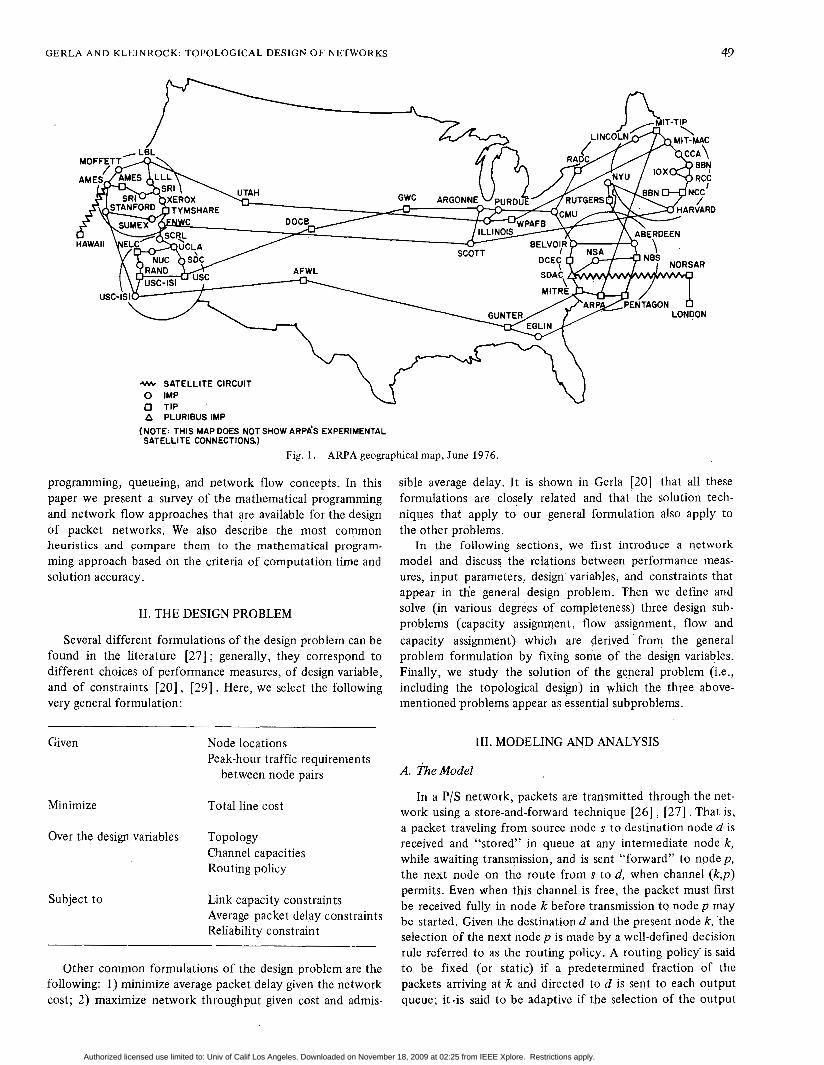
together as a resource-sharing network [32]. Among the shared resources we include: computer power (for load sharing); specialized hardware; specialized software; and data files. This type of network differs from the former in that the computer resources are distributed among the nodes, rather than accumulated in a central node; this configuration is here referred to as a distributed computer network. One of the first examples of a distributed network is represented by the ARPANET, a recent configuration of which is shown in Fig. 1.

In distributed networks traffic demands can arise between any two nodes of the network, and not only between terminals and the “central” node. Consequently, better cost- effectiveness and performance are achieved with topological configurations which present a higher degree of connectivity than the centralized tree structures 1201.

Computer network users share not only processing facilities, but also communication facilities [30] . The cost-effective configuration and use of communication channels is the main concern of this paper. Conventional line-switching techniques, as used by the common carrier switching network, in which a dedicated path is established for each conversation, are ineffi- cient for computer communications in a bursty mode (e.g., terminal-to-computer conversations). In fact, with the present technology, the time required for establishing and clearing (disconnecting) the path is much longer (on the order of seconds) than the average intercomputer conversation. A more efficient solution for line sharing and speed conversion in a bursty data communication environment is provided by. the packet-switching (P/S) technique 1271. Each message is seg- mented into packets at the source; these packets, instead of traveling along paths reserved in advance, adaptively find their way through the network independently, in a store-and-forward fashion. More than one route between source and destination may be used; such routes can be thought of as pipelines, along which several packets may travel simultaneously, interleaved with other packets corresponding to different source-destination pairs. It is through this pipelining and interleaving that large improvements in network thoughput and message delay are achieved.

The design of distributed P/S networks is substantially different and more complex than the design of centralized networks. The presence of more than one route between each origin and destination in the distributed case requires the solution of complex routing and capacity allocation problems; furthermore, the use of P/S techniques requires the analysis of the relationship between packet delay and line and buffer utilization.

Several algorithms have been proposed for the design of distributed networks. Some of the algorithms are of a heuristic nature; some others are based on more rigorous mathematical

Authorized licensed use limited to: Univ of Calif Los Angeles. Downloaded on November 18, 2009 at 02:25 from IEEE Xplore. Restrictions apply.

GERLA AND KLEINROCK: TOPOLOGICAL DESIGN OF NETWORKS 49

-w+ SATELLITE CIRCUIT 0 IMP 0 TIP A PLURIBUS IMP

SATELLITE CONNECTIONS.) (NOTE: THIS MAP DOES NOT SHOW ARPA’S EXPERIMENTAL

Fig. 1. ARPA geographical map, June 1976.

programming, queueing, and network flow concepts. In this paper we present a survey of the mathematical programming and network flow approaches that are available for the design of packet networks. We also describe the most common heuristics and compare them to the mathematical programming approach based on the criteria of computation time and solution accuracy.

11. THE DESIGN PROBLEM

sible average delay. It is shown in Gerla [20] that all these formulations are closely related and that the solution techniques that apply to our general formulation also apply to the other problems.

In the following sections, we first introduce a network model and discuss the relations between performance measures, input parameters, design’ variables, and constraints that appear in the general design problem. Then we define and solve (in various degrees of completeness] three design subproblems (capacity assignment, flow assignment, flow and

Several different formulations of the design problem can be capacity assignment) which are derived . from the general found in the literature [27] ; generally, they correspond to problem formulation by fixing some of the design variables. different choices of performance measures, of design variable, Finally, we study the solution of the general problem (i.e., and of constraints [20], [29]. Here, we select the following including the topological design) in which the three above- very general formulation: mentioned problems appear as essential subproblems.

Given Node locations Peak-hour traffic requirements

between node pairs

Minimize Total line cost

Over the design variables Topology Channel capacities Routing policy

Subject to Link capacity constraints Average packet de1,ay constraints Reliability constraint

Other common formulations of the design problem are the following: 1) minimize average packet delay given the network cost; 2) maximize network throughput given cost and admis-

111. MODELING AND ANALYSIS

A. l;heModel

In a PIS network, packets are transmitted through the network using a store-and-forward technique [26] , [27] . That is, a packet traveling from source node s to destination node d is received and “stored” in queue at any intermediate node k, while awaiting transmission, and is sent “forward” to node p , the next node on the route from s to d, when channel (k ,p) permits. Even when this channel is free, the packet must first be received fully in node k before transmission to node p may be started. Given the destination d and the present node k, ‘the selection of the next node p is made by a well-defined decision rule referred to as the routing policy. A routing policy’is said to be fixed (or static) if a predetermined fraction of the packets arriving at k and directed to d is sent to each output queue; it .is said to be adaptive if the selection of the output


50 IEEE TRANSACTIONS ON COMMUNICATIONS, JANUARY 1977

channel at each node depends on some estimate of current network traffic [27].

Traffic requirements between nodes arise at random times and the size of the requirement is also a random variable. Con- sequently, queues of packets build up at the channels and the system behaves as a stochastic network of queues. For routing purposes, packets are distinguished only on the basis of their destination E171 , [20] , [27] ; thus, messages having a common destination can be considered as forming a “class of customers.” The P/S network, therefore, can be modeled as a network of queues with n classes of customers where n is the number of different destinations [29] .

B. Delay Analysis A vital performance measure for a computer-communica-

tion network is the average source-to-destination packet delay T, defined as follows 1271 :

j S . k ..

where

Y j k average packet rate flowing from source j to desti-

z j k average packet delay (queue and transmission) from nation k

j to k

A straightforward application of Little’s result [28], [29] to the network of queues model leads to tbp foilowing very useful expression for T:

(31

where b is the number of links (arcs), X i is the average traffic rate, and Ti is the average queueing plus transmission delay on link i. Thjs expression, establided by Kleinrgck in 1964’[27], i s very general (as general as Little’s result!), and extremely simple. Unfortunately, we are not able in general to evaluate hi and Ti. However, if we make the following assumptions: 1) external Poisson arrivals; 2) exponential packe’t length distribution; 3) infinite nodal storage; 4) fixed routing; 5) error- free channels; 6) no nodal delay; and 7) independence bytween interarrival times and transmission times on each channel, then the evaluation of (3) can be carried out analytically [26], [27]. In fact, the network of queues reduces to the model first studied by Jackson [23], in which each queue behaves as an independent M/M/1 queue [28]. Thus, the average delay Ti on channel i is given by

(4)

l/p average packet length (bits/packet) Ci capacity of channel i (bitsls) hi average packet rate on channel i (packetsls).

The average rates hi are easily computed from the routing tables and the traffic requirement matrix [20], [27] .

By substituting (4) into (3 ) and lettingfi be the average bit rate on channel i (bits/s), we obtain the following expression for T:

Although the delay expression (5) is sufficiently .accurate for most design purposes, it is possible to obtain expressions which correspond more accurately to measured results. Klein- rock proposed in [25] the following very general formula, which includes propagation and nodal processing delay:

1 b

Y i = l T = - x hi[Ti + P i + Ki]

where

Pi propagation delay in channel i (seconds) Ki nodal processing time in the node at which channel i

terminates (s/packet).

The term Ti depends on the nature of the traffic and on the packet length distribution.

Finally, assuming a general packet length distribution, with mean 1/p and variance u2, we obtain [26] :

where 0 = (1 + p2u2)/2. An even more detailed model has been recently proposed and is discussed in [31].

The validity of the above assumptions and approximations has been tested and verified through .simulation and measure- ments by many authors in a variety of applicatipns [17], [25], [27] 1311. The results indicate that the model is robust. ” In this paper, without loss of generality, we limit our con- siderations to the delay expression in (5). Most of the techniques described in the sequel can be easily extended to more elaborate delay expressions. Furthermore, the solution of some of the design problems seems to be rather insensitive to the introduction of additional detailsin the delay formula [20] .

C. The Communications Cost With Ci the capacity of link i, we let di(Ci) be the cost of

leasing capacity value.Ci for link i. The communication cost D is defined as

b

D = di(Ci). i = l

where The availability and effectiveness of the design algorithms depends rather critically upon the form for di(Ci). In most



applications di(Ci) is a discrete variable; however, for computational efficiency it is often convenient to approximate the discrete costs with continuous costs during the initial optimization phase, and to discretize the continuous values during a refinement phase [25].

D, Traffic Requirements Average (busy-hour) traffic requirements between nodes

can be represented by a requirement matrix R = { r j k } , where rjk is the average transmission rate from sourcej to destination k. In some cases, we define the requirement matrix as R = pR, where R is a known basic traffic pattern and p is a variable scaling factor usually referred to as the traffic level.

In general, R (or E ) cannot be estimated accurately a priori, because of its dependence upon network parameters (e.g., allocation of resources to computers, demand for resources, etc.) which are difficult to forecast and are subject to changes with time and with network growth. Fortunately, the analysis of several different traffic situations has shown that the optimal design is rather insensitive to traffic pattern variations [ l ] , [20] . This insensitivity property, which seems to be typical of distributed networks, justifies the use of traffic averages for network design.

E. Routing Policy In designing network topologies, one generally assumes

fixed routing, since fixed routing is easy to describe (by means of routing tables, for example) and allows the direct evaluation of channel flows and average delay as a function of routing tables and traffic requirements. Adaptive routing, on the other hand, is complex to describe, and requires simulation to evaluate channel flows and delay. Furthermore, it was shown that at steady state, flow patterns and delays induced by good adaptive routing policies are very close to those obtained with optimal fixed policies [18] . This fact suggests that network configurations optimized with fixed routing, are also (near) optimal for adpative routing operations [27] .

I;: Link Flows The routing policy and the traffic requirements uniquely

determine the vector f (fi,fi, .-, f b ) where f i is the average data flow on link i. The evaluation o f f is straightforward in the case of fixed routing; it can, at this point, only be obtained by simulation if the routing is adaptive.

Conversely, not any generic vector f corresponds to a realizable routing policy and requirement matrix. If it does, then f is a multicommodity (MC) flow for that particular requirement matrix. An MC flow results from the sum of single commodity flows f j k (j,k = 1,2, -., n ) where f j k is the average flow vector generated by packets with source node j and destination node k, and n is the number of nodes. Clearly, each single commodity flow of the MC flow must separately satisfy nonnegativity and flow conservation constraints.

G. The Capacity Constraint

The presence of capacity constraints f < C (where C = (c1,C2, .-, cb)) makes the design problem in Section 11 a constrained MC flow problem. From the delay expressions (4)

and (7), we notice that if the link flow approaches the link capacity, then the delay approaches infinity, thus violating the delay constraint [ 161 . Therefore, if both capacity and delay constraint must be satisfied the capacity constraint is implied by the delay constraint and can be disregarded.

H Reliability Links and nodes in a real network can fail with nonzero

probability, thus interrupting some communication paths. It is important to evaluate the overall network reliability in the presence of such failure probabilities.

Several reliability measures have been proposed for computer-communication networks. Among them we mention: the probability of the network being connected (PC); and the fraction of communicating node pairs (FR). Such measures must be verified during the design phase.

Van Slyke and Frank developed very efficient techniques for the evaluation of PC and FR [36] . The techniques, however, are based on simulation and are too time-consuming to be included in a global design algorithm.

Roberts and Wessler [32] proposed as a reliability measure, the two-connectivity of the network (i.e., two node-disjoint paths available between each node pair). This measure is easy to include as a constraint in the topological design. Further- more, it is adequate for networks with a relatively small number of nodes (on the order of 20-40) and relatively small component failure probability (on the order of 0.01).

For larger networks (or higher failure rates), stronger constraints must be applied to the network topology (e.g., three- connectivity, no long chains, etc.) in order to obtain adequate reliability.

This concludes our model description. In the next four sections, we discuss some of the important design problems and their solutions.

IV. THE LINK CAPACITY ASSIGNMENT (CA) PROBLEM

A. Problem Formulation

The CA problem can be formulated as follows:

Given

Minimize

Topology Requirement matrix R Routing policy (and therefore

link flow vector f = ( f l , f i , ' ' ' 2 f b 1)

b

D = x di(Ci) i= 1

Over the design variables c = (cl, c2, ..., cb)

Subject to f < C



The optimal assignment of capacities to a distributed network with arbitrarily fixed routes is not very interesting as a stand-alone problem, since routing plays a determinant role in the optimization of network performance. Rather, the CA is of practical interest as subproblem of more general optimization problems.

The technique used for the solution of the CA problem depends on the nature of the cost-capacity functions di(Ci). In the following, we present optimal and suboptimal algorithms for linear, concave, and discrete costs.

B. Linear Costs Assuming that di(Ci) = diCi + dio where dio is a positive

start-up cost, the optimal solution is obtained using the method of Lagrange multipliers [27]. In particular, the optimal capacity for channel i is given by

and the minimum cost D is given by

D = b [ difi + dio + (g-y] i = l YTm a x

C. Concave Costs The concave case can be solved iteratively by linearizing the

costs and solving a linearized problem at each iteration [20]. The method leads, in general, to local minima. However, for the very important case of a power law cost function (i.e., di(Ci) = diCia + dio where 0 < QI < l), Kleinrock showed that there exists a unique local minimum [25]. The iterative procedure therefore yields the optimal solution in the power law case.

D. Discrete Costs

The optimal solution to the discrete CA problem can be obtained with a dynamic programming (DP) technique. The DP algorithm, described by Gerla in [20] , requires an amount of computation which, in most applications, is close to (b )2 . Another suboptimal technique for the solution of the discrete CA problem is the Lagrangian decomposition (LD). The ‘LD method, first developed by Everett [ 9 ] , and subsequently improved by Fox [ 101 and Whitney [37] , is suboptimal in the sense that it determines only a subset of the set of optimal solutions corresponding to various values of the parameter T,,,. The amount of computation required by LD is slightly more than linear with respect to the number of arcs b.

The delay versus cost plot in Fig. 2 shows DP and LD solutions for a large range of values of Tmax for a discrete CA application relative to a 26-node ARPANET topology [20]. The circles correspond to LD solutions, whereas the union of circles and dots corresponds to DP solutions. As a property of the LD method, the LD solutions belong to the convex envelope of the global set of optimal DP solutions.

V. THE ROUTING PROBLEM

A. Problem Definition

The routing problem is here defined as the problem of finding the fixed routing policy which minimizes the average delay T. A possible formulation of the problem is the following: -

Given Topology Channel capacities {Ci} Requirement matrix R

Minimize

Over the design variable f = (fi, fi, fb)

Subject to a) f is a multicommodity flow satisfying the requirement matrix R

b ) f < C

From formulation (12), we notice that the routing problem is a convex MC flow problem on a convex constraint set; therefore, there is a unique local minimum, which is also the global minimum and can be found using any downhill search technique [5] .

Several optimal techniques for the solution of MC flow problems are found in the literature [ 8 ] , [ 3 5 ] ;however, their direct application to the routing problem proves, in general, to be cumbersome and computationally not efficient. Conse- quently, considerable effort was spent in developing heuristic suboptimal routing techniques [5] , [17] , [33] . Satisfactory results were obtained and computational efficiency was greatly improved. However, all of these techniques are affected by various limitations and may fail in some pathological situations.

A new downhill search algorithm, called flow deviation (FD), was recently developed by Fratta, Gerla, and Kleinrock [16] . The FD algorithm finds the optimal solution and is computationally as efficient as the heuristics. To place the FD algorithms in the proper perspective we first introduce the most popular among the heuristic algorithm-the “minimum link” algorithm-and compare it to the FD algorithm.

B. The Minimum Link Algorithm We begin by giving an outline of the heuristic algorithm

reported in [5] . Algorithm:

Step I: For a given sourcej and destination k, determine all paths I I j h with the minimum number of intermediate nodes. Such paths are called “feasible” paths.

Step 2: Choose, among the feasible paths, the least utilized path (or the path with maximum residual capacity).



.04 I I I I I I I I I I I I I I I I I 1 102 66 70 74 78 82 86 90 94 98

COST (K$/month)

Fig. 2. Delay versus cost for discrete capacity assignments on 26-node 30-link topology.

Step 3: Route the requirement Y j k along such a path. Step 4: If all source destination pairs have been pro-

cessed, stop; otherwise select a new pair and go to 1. Step 1, repeated for all node pairs, corresponds to the

evaluation of all shortest paths between all pairs of nodes, assuming unitary link length. Such a computation requires from (n)2 to (n)2 log (n) operations, depending on network connectivity. I t can be shown that the total amount of computation required by the algorithm has proportion between (n)2 and (n)2 log (n).

The minimum link algorithm is conceptually simple and computationally very efficient. Its major drawback is that of being rather insensitive to queueing delays and therefore possibly far from optimum in heavy traffic situations.

Step 2: Let xp be the minimizer of T[(1 - h)4(p) 4- X f ( p ) ] , O ~ X ~ 1 . L e t f ( ~ + 1 ) = ( 1 - ~ ~ ) ~ ( ~ ) + x ~ ; p f ( P ) .

Step 3: If I T(f(~+1)) - T(f(p)) I < e, stop: f(p) is optimized to within the given tolerance. Otherwise let p = p + 1 and go to Step 1. A geometric representation of the FD algorithm is given in Fig. 3.

Step 1 is the most time-consuming operation of the algorithm, and requires an amount of computation between (n)2 and (n)2 log (n). Therefore, the amount of computation required by the minimum link algorithm and the FD algorithm are comparable. A typical central processing unit (CPU) requirement is from 2 to 4 seconds for a 30-node application on a large computer.

C. The Flow Deviation Algorithm VI. THE CAPACITY AND FLOW ASSIGNMENT (CFA)

Before introducing the FD algorithm, we mention the following properties of the optimal routing solution.

Property 1: The set of MC flows f satisfying the requirement matrix R is a convex polyhedron. The extreme points of such a polyhedron are called “extremal flows” and correspond to shortest route policies. A shortest route policy is a policy that routes each (j,!) commodity along the shortest ( j k ) path, evaluated under an arbitrary assignment of lengths to the links. To each such assignment there corresponds an extremal flow and conversely. Any MC flow can be expressed as a convex combination of extremal flows [ 161 .

Property 2: For a given MC flow f, let us define link length as a function of link flow of the form li 4 aT/afi. Let 4 be the shortest route flow associated with such link lengths and let


The CFA problem can be formulated as follows:

Given Topology Requirement matrix R Cost-capacity functions di(ci)

Minimize

Over the design variables f, C

f’ = (1 - A)@ + Xf be the convex combinations of 4 and f minimizing the delay T. If T ( f ) = T ( f ) , then f is optimal.

Property 2 provides a way of finding a downhill direction, ‘if it exists. Based on such property, we may now state the FD algorithm, as follows.

Such that a) f is an MC flow satisfying the requirement matrix R

b ) f < C 1 f i C)TV,O=-x-

Algorithm: Y i = l ci -fi Step 0: Let f (0) be a starting feasible flow. (A starting

feasible flow can be obtained using a modified version of the FD algorithm [ 161 .) Let p = 0.

Step 1: Compute q5(p), the shortest route flow corre- The CFA problem requires the simultaneous optimization sponding to lib) = [aT/afi],=,(,), Vi = 1, .-, b. of routes and line capacities. The existence of a huge number

Tmax



Fig. 3. Geometrical representation of the FD algorithm. Characters with tildes beneath are boldface in text.

of local minima makes the exact solution difficult to obtain. Therefore, we discuss here only suboptimal techniques.

B. Linear Costs. In the linear cost case we can obtain, for a givenf, a closed

form expression of the optimal C in terms o f f [see (9)] . In particular, the total cost D can be expressed in terms o f f only, and problem (1 3) can be reformulated as follows:

Given Topology Requirement matrix R

r Minimize

Fig. 4. Cvncave objective functionDCf). Characters with tildes beneath are boldface in text.

The convergence follows from the fact that there are only a finite (albeit large) number of extremal flows and repetitions are not allowed because of the stopping rule 2.

From (14) the equivalent length li defined in Step 1 has the following expression:

L

Over the design variable f

Such that f i s an MC flow satisfying R

It can be shown that D ( f ) is concave over the convex polyhedron of feasible multicommodity flows [20] . This implies that there are in general several (in fact, enormous numbers of) local minima corresponding to some corners of the polyhedron, i.e., corresponding to some extremal flows (see Fig. 4). The FD method described in the previous section can still be applied, in a properly modified form; however, it leads to local minima. More precisely, the FD algorithm performs a local search on extremal flows, until it finds a local minimum. The modified FD algorithm is next introduced.

FD algorithm (for concave objective function): Step 0: Let f(O) be a feasible starting flow. Let p = 0. Step I : Let f@+l) be the extremal flow corresponding

to the following definition of equivalent lengths:

Step 2: I f D(f@+l)) .> D ( f ( p ) ) , stop: f (p) is a local minimum. Otherwise, let p = p + 1 and go to 1 .

Notice that limfi-o li = 00. This implies that whenever the flow (and therefore the capacity) of link i is reduced to zero at the end of an iteration, flow and capacity will remain zero f o r all subsequent i terat ions, s ince the incrementa l cost of restoring the flow on a link is proportional to Zi which in this case is infinity. In ‘other words, uneconomical links tend to be eliminated by the algorithm. This link elimination property, first observed by Yaged [38], can be utilized in the topological design, as shown in the following section.

The solution obtained with the FD algorithm is a local minimum which depends on the selection of the starting flow f ( O ) . In order to obtain a more accurate estimate of the global minimum, several locals are usually explored, starting from randomly chosen flows.

C. Concave Costs For concave channel costs there is no closed-form expres-

sion of D in terms of f . However, it has been shown by Gerla that D ( f ) is concave over f, and that the FD algorithm can be still applied to obtain local minima 1201 .

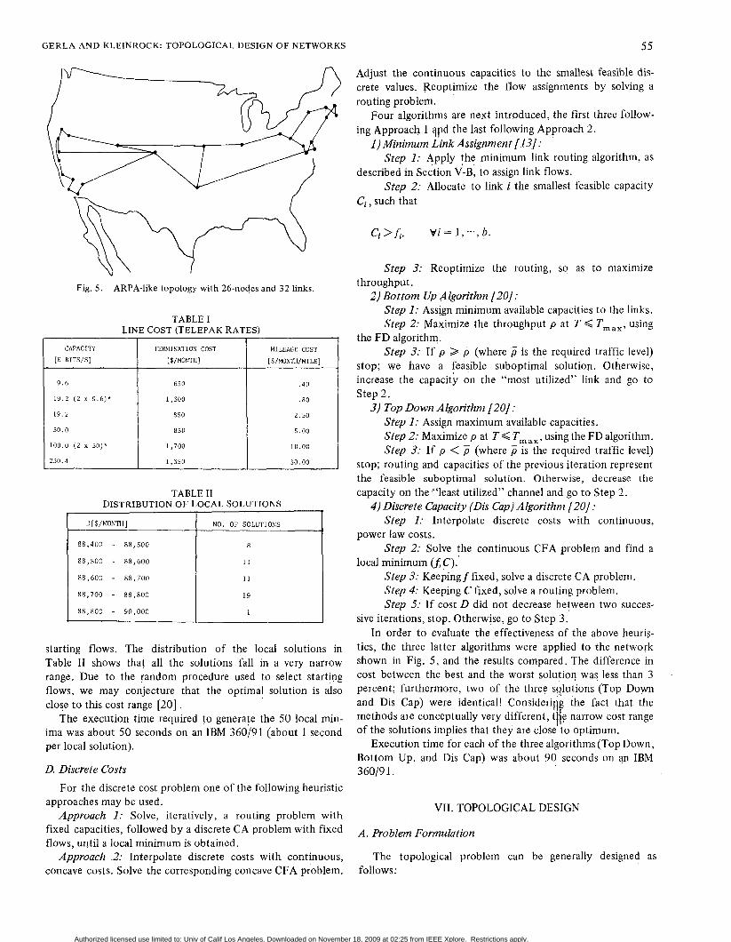
An application of the FD method to the topology shown in Fig. 5 is next introduced. Channel capacities are available only in discrete sizes (see Table I); therefore, discrete channel costs are approximated with continuous power law costs, to apply the concave cost version of the FD algorithm.

A uniform traffic requirement of 1 kbit/s was assumed between all node pairs. Fifty different local minima were obtained with the FD method using randomly generated


GERLA AND KLEINROCK: TOPOLOGICAL DESIGN OF NETWORKS

f?+ Fig. 5 . ARPA-like topology with 26-nodes and 32 links.

TABLE I LINE COST (TELEPAK RATES)

CAPACITY I TERJIINATION COST [K RITS/S] [$/MONTH1

9.6

1,300 19.2 (2 x 9.6)’

650

850 19.2

100.0 (2 x SO)* 1,700

230.4 1,350

MILEAGE COST [$/MONTH/MILE]

.40

.80

2.50

5.00

10.00

30.00

TABLE I1 DISTRIBUTION OF LOCAL SOLUTIONS

1

D[$/MONTH] NO. OF SOLUTIONS

88,400 - 88,500 8

88,500 - 88,600

88,600 - 88,700

11

11

starting flows. The distribution of the local solutions in Table I1 shows that all the solutions fall in a very narrow range. Due to the random procedure used to select starting flows, we may conjecture that the optimal solution is also close to this cost range [ 2 0 ] .

The execution time required to generate the 50 local minima was about 50 seconds on an IBM 360/91 (about 1 second per local solution).

D. Discrete Costs For the discrete cost problem one of the following heuristic

approaches may be used. Approach 1: Solve, iteratively, a routing problem with

fixed capacities, followed by a discrete CA problem with fixed flows, until a local minimum is obtained.

Approach 2 : Interpolate discrete costs with continuous, concave costs. Solve the corresponding concave CFA problem.

5 5

Adjust the continuous capacities to the smallest feasible discrete values. Reoptimize the flow assignments by solving a routing problem.

Four algorithms are next introduced, the first three following Approach 1 ?pd the last following Approach 2.

1)Minimum LinkAssignment [13]: Step I: Apply the minimum link routing algorithm, as

Step 2: Allocate to link i the smallest feasible capacity described in Section V-B; to assign link flows.

Ci , such that

Ci > fi, V i = 1, -., b .

Step 3: Reoptimize the routing, so as to maximize throughput.

2) Bottom Up Algorithm [20]: Step 1: Assign minimum available capacities to the links. Step 2: Maximize the throughput p at T < Tmax, using

the FD algorithm. Step 3: If p 2 5 (where 5 is the required traffic level)

stop; we have a feasible suboptimal solution. Otherwise, increase the capacit; on the “most utilized” link and go to Step 2.

3) Top Down Algorithm /20] : Step I: Assign maximum available capacities. Step 2: Maximize p at T < TmaX, using the FD algorithm. Step 3: If p < 5 (where 6 is the required traffic level)

stop; routing and capacities of the previous iteration represent the feasible suboptimal solution. Otherwise, decrease the capacity on the .“least utilized” channel and go to Step 2.

4 ) Discrete Capacity (Dis Cap) Algorithm [20] : Step 1: Interpolate discrete costs with continuous,

Step 2: Solve the continuous CFA problem and find a

Step 3: Keepingf fixed, solve a discrete CA problem. Step 4: Keeping C fixed, solve a routing problem. Step 5: If cost D did not decrease between two succes-

sive iterations, stop. Otherwise, go to Step 3. In order to evaluate the effectiveness of the above heuris-

tics, the three latter algorithms were applied to the network shown in Fig. 5 , and the results compared. The difference in cost between the best and the worst solution was less than 3 percent; furthermore, two of the three sqlutions (Top Down and Dis Cap) were identical! Consideriqf: the fact that the methods are conceptually very different, the narrow cost range of the solutions implies that they are close to optimum.

Execution time for each of the three algorithms (Top Down, Bottom Up, and Dis Cap) was about 90 seconds on an IBM 36019 1.

power law costs.

local minimum (LC).

VII. TOPOLOGICAL DESIGN


The topological problem can be generally designed as follows:



Given

Minimize

Such that

Requirement matrix R

where the set of arcs A specifies the topology

a) f is an MC flow satisfying the

b ) f < C requirement matrix R

d) The set A must correspond to a 2-connected topology

There exists no efficient technique for the exact solution of this topological problem. Several heuristics, however, have been proposed and implemented and are discussed below.

B. The Branch X-Change (BXC) Method [ 131, [34J

This method starts from an arbitrary topological configuration and reaches local minima by means of local transformations (a local transformation, often called branch X-change, consists of the elimination of one or more old links and the insertion of one or more ne'w links).

The BXC method has found applications in a variety of topological problems (natural gas pipelines [ 111 , minimum cost survivable networks [34], centralized computer networks [12] , etc.). In particular, BXC has been applied to the topological design of distributed computer networks [13] . The algorithm described in [ 131 is iterative'and each iteration consists of three main steps, as follows.

Step I: Local transformation. A new link is added and an old link is deleted in such a way that two-connectivity is maintained.

Step 2: Capacities and flows are assigned to the new topological configuration using the minimum link assignment described in Section VI, and cost and throughput are evaluated. If there is a cost-throughput improvement, then the topological transformation from Step 1 is accepted. Otherwise, it is rejected.

Step 3: If all local transformations have been explored, stop. Otherwise, go to Step 1.

C. Concave Branch Elimination (CBE) Method (201, (38J The CBE method can be applied whenever the discrete

costs can be reasonably approximated by concave curves [20] . The method consists of starting from a fully connected topology, using concave costs and applying the FD algorithm described in Section VI until a local minimum is reached. Typically, the FD algorithm eliminates uneconomical links, and strongly reduces the topology. Once a locally minimal topology is reached, the discrete capacity solution can be obtained from the continuous solution with the techniques discussed in Section VI. Since two-connectivity is required, the FD algorithm is terminated whenever the next link removal

violates this constraint; the last two-connected solution is then assumed to be the local minimum. In order to obtain several local minima, and therefore several different topological solutions, the FD algorithm is applied to several randomly chosen initial flows.

D. Other Methods

Both the BXC and CBE methods have some shortcomings. For example, the BXC method requires an exhaustive explora- tion of all local topological exchanges and tends to be very time consuming when applied to networks with more than 20 or 30 nodes. The CBE method, on the other hand, can very efficiently eliminate.uneconomica1 links, but does not provide for insertion of new links. In order to overcome such limitations, new methods derived from BXC or CBE have been recently proposed and are now being investigated.

The cut-saturation method, discussed in [22], can be considered as an extension of the BXC method, in the sense that, rather than exhaustively performing all possible branch exchanges, it selects only those exchanges that are likely to improve throughput and cost. In particular, at each iteration: a routing problem is solved; the saturated cut (i.e., the minimal set of most utilized links that, if removed, leaves the network disconnected) is found and a new link is added across the cut; then the least utilized link is removed. The selection of the links to be inserted or removed depends also on link cost.

The concave branch insertion method, discussed in [20], identifies and introduces links which provide cost savings under a concave cost structure. The method can be efficiently combined with the CBE method, to compensate for the inability of the latter to introduce new links.

In some applications with very irregular distributions of node locations, or with constraints which are difficult to formulate analytically (e.g., no chains longer than m hops; connectivity higher than 2, etc.), network design can be greatly enhanced using man-computer interaction. To this end, interactive design programs have been developed in which the network designer can observe (and eventually correct) the topological transformations performed by the computer and displayed iteration after iteration on a graphic terminal.

In general, the selection of the appropriate algorithm will depend on the cost-capacity structure, on the presence of additional topological constraints, on the degree of human interaction allowed and, finally, on the tradeoff between cost and precision required by the particular application.

E. Bounds

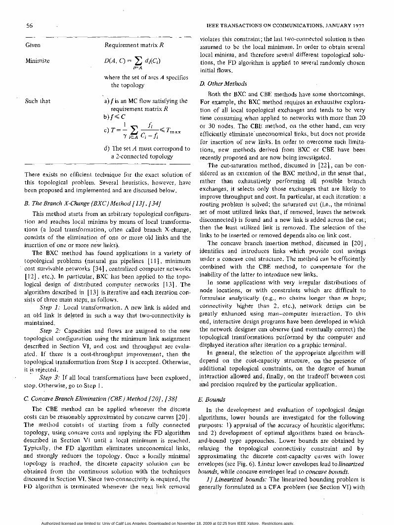
In the development and evaluation of topological design algorithms, lower bounds are investigated for the following purposes: 1) appraisal of the accuracy of heuristic algorithms; and 2 ) development of optimal algorithms based on branch- and-bound type approaches. Lower bounds are obtained by relaxing the topological connectivity constraint and by approximating the discrete cost-capacity curves with lower envelopes (see Fig. 6). Linear lower envelopes lead to linearized bounds, while concave envelopes lead to concave bounds.

1) Linearized bounds: The linearized bounding problem is generally formulated as a CFA problem (see Section VI) with


GERLA AND KLEINROCK: TOPOLOGICAL DESIGN OF NETWORKS

l2 t 57

0

C1 c2 c3 = %Ax Capacity

Fig. 6 . Linear and concave lower envelope.

linear line costs and fully connected topology. The direct solution of the bounding problem is difficult because of the concavity of the objective function D(f) [see (14)]. Rather, the objective D ( f ) is further bounded as follows:

where Cmax = max admissible link capacity option. The lower bound DLB(f) in (16) is convex. Thus, a lower

bound to the topological problem is obtained by minimizing the convex objective DLB(f) using the FD method.

The procedure as defined above applies to the case in which no link (and link capacity) is preassigned; but can be extended to applications in which a set of links is assigned a priori, and new links must be added in order to meet the requirements (e.g., network expansion problem) [39] .

The linearized bound can also be applied in branch-and- bound (B-B) algorithms [39]. To this end, recall that at each step of a B-B algorithm a bound is required on the cost of a partially specified topology with a set n, of assigned links, a set np of potential links, and a set ne of excluded links. This bounding problem is similar to the topological design with some preassigned links, and can be approached with the linearized bounding procedure previously mentioned.

2 ) Concave 'bounds: Linearized bounds are simple and exact. However, they are often too loose, especially if line cost versus capacity shows strong economy of scale, or more generally, the cost-capacity structure cannot be accurately bounded with a linear envelope. In such cases, concave bounds lead to better results.

Unfortunately, the presence of concave link costs makes the solution of the bounding problem difficult, since the objective D ( f ) cannot be expressed in closed form (see Section VI-C). One possible (but complex) approach consists 9f formu- lating linear or convex bounds for D ( f ) , and then solving the problem exactly with the FD method. A simpler approach,

0 f- 305 MILES A 4- 100 MILES 0 4- 10 MILES

0 1 I I I L

0 50 1M) 150 200 C (kbiils)

Fig. 7. Concave approximations to link costs, for various link lengths (Telpak tariff assumed).

which .we follow, consists of finding an approximate solution to the bounding problem with the technique indicated in Sec- tion VI-C. The lower bound is then derived from the approximate solution taking into account the accuracy of the solution method. For example, if D is the cost of the approximate solution and E is the relative accuracy, the lower bound is DL, = D(1 - E ) .

VIII. APPLICATIONS

We now evaluate the efficiency of some of the heuristic techniques as applied to the topological design of a proposed 26-node ARPANET configuration (see Fig. 5 ) . Capacity options vary from 9.6 to 230.4 kbit/s; discrete cost-capacity functions as well as concave approximations are shown in Fig. 7. Delay requirement is Tmax = 200 ms. Traffic demands are uniformly distributed between node pairs. Several levels of throughput requirement in the range from 400 to 700 kbit/s are considered.

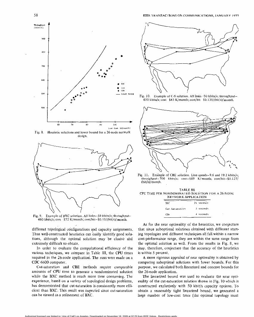
The suboptimal solutions obtained with different techniques are displayed in a throughput versus cost diagram in Fig. 8. For each technique several solutions were generated at different throughput levels. Since each technique typically generates several locally optimal solutions, only the non- dominated solutions were shown in Fig. 8. (Note: SolutionA is defined to be dominated by Solution B if B has lower cost and better performance than A . ) Figs. 9 , 10, and 11 display some typical topologies obtained with BXC, cut-saturation, and CBE, respectively.

From Fig. 8, it is noticed that different techniques lead to solutions which fall in a narrow cost-throughput range. The resulting topological structures, on the other hand, may vary considerably from technique to technique, as can be seen by comparing cut-saturation and CBE solutions in Figs. 10 and 11, respectively. Cost and throughput of the two solutions are approximately the same, but cut-saturation yields about 30 links while CBE yields about 60 links. We note that the marginal cost [dollars/(bit/s)/month] varies over a moderate range for these three procedures.

These facts lead us to conjecture that there are a large number of low-cost solutions which may correspond to very


1977 On the Topological Design of Distributed Computer Networks the... · · 2010-01-18On the...

Documents

Transcript of 1977 On the Topological Design of Distributed Computer Networks the... · · 2010-01-18On the...