THEORY OF PROBABILITYVolume XVI AND ITS APPLICATIONS Number4

1971

PROBABILITY INEQUALITIES FOR SUMS OF INDEPENDENTRANDOM VARIABLES

D. KH. FUK AND S. V. NAGAEV

(Translated by B. Seekler)

0. Introduction

In [1], S. V. Nagaev obtained the following estimate for large deviationprobabilities for the case of identically distributed independent randomvariables X, ..., X, with EX O, DX 1"

where x > 0, y > O,A EIXI < ,t > 2andK 1 + e-t(t + 1)t+2.This paper is devoted to improving this result and to extending it to

the case of non-identically distributed independent random variables forwhich the existence of finite moments ofsome particular order is not assumed.In Section 1, certain inequalities are derived whose right-hand sides consistof two components the sum of the probabilities of the tails and a componentcontaining truncated moments. In Section 2, the proofs of these inequalitiesare given. A bilateral inequality is stated in Section 3. Special cases areconsidered in Section 4. Section 5 deals with examples involving the compu-tation of the probabilities and Section 6 contains applications to the stronglaw of large numbers.

Let X, ..., X, be non-identically distributed independent randomvariables (i.r.v.) with respective distribution functions F(u),..., F,(u). Set

S=X +... +X.

Throughout the following x is an arbitrary prescribed positive number,Y {y, ..., y.} is a set of n positive numbers and y >__ max{y, -.-, y.}.

A(t;.,. ), B2(., and #(., .) are to denote, respectively, the sum of theabsolute moments of order t (specified within the parentheses), the variancesand the means truncated at the levels specified within the parentheses.The letter Ydesignates summation over from 1 to n ofthe moments truncated

643

644 D. Kh. Fuk and S. V. Nagaev

at levels Y l, "’", Y,. For example,

(t; Y, o) lul

B2(- K u2 dFi(u), ,(- , u dFi(u).

Theorem 3 stated in Section 1 and the results of Section 6 are jointefforts while the remaining results are due to D. Kh. Fuk.

I. Unilateral Inequalities

Theorem 1. Let 0 < t < 1. Then

(1) P{S. x} P{X >= Yi} + P1,i=1

where

(2) P1 exp log + 1y y A(t; O, Y)

(3) xyt- > A(t;0, Y),

then

(4) P{S,>=x} <= Z P{X, >= y,} + P2,i=1

where

(5) P2 expx A(t, O, Y) xlog

y yt y

and P2 <= P1.

Theorem 2. Let <_ < 2. Then

(6) P{S. _> x} =< Z P{Xi > Yi} + P3,i=1

where

(7) P3 exp + ytY

xyt-log

A(t Y, Y)

Probability inequalitiesfor sums ofindependent random variables 645

(8)

(9)

(10)

We now go over to the case >= 2 and we let

P4 expY

x u(- Y, Y)) log

Ps =exp fl----- --Y A(t O, Y)

P(-Y’y Y))log( A(t O, Y)

x(x/2 #(-Y, Y))}P6 expetB2(_ Y, Y)

(11)

then

Theorem 3. Let t >= 2, 0 < cz < 1 and fl 1 a. If

max t. logA(t;0.

+ 1etB2(_ Y, lO

(12)

(13)

P{S. __> x} =< P{X, >= y,} + P.i=1

P{S. >= x} =< Z P{Xi >= Y,} +i=1

(14) max It. log

then

A(t; O, Y)+ 1 >

etB2(_ Y, lO

(15) P{S. _>_ x} _< P{X, Yi} + P6"i=1

Theorem 3’. For t 2, 0 < < 1 and fl 1- , the assertions ofTheorem 3 hold with the quantities B2( Y, Y) and (-Y, Y) replaced byB2( , Y)and #(-, Y), respectively.

Theorem 4. The following inequality holds"

(16) P{S. >= x} =< P{X, >__ y} + P7,i=1

where

(17) P7=exp bt(-’Y)+ log +1y y B2(- z, Y)

REMARK 1. There are inequalities for P{S. __< -x} which are left-sidedanalogues of the inequalities obtained in Theorems 1-4. The quantities.=, P{X >= y}, A(t;-0, Y), S2( c, Y), p(-Y, Y)and #(-c, Y) on theright-hand sides of the latter have to be replaced by

__P{X <= -y},

646 D. Kh. Fuk and S. V. Nagaev

A(t; Y, 0), B2( Y, oo), -#(- Y, Y) and -#(- Y, oe), respectively; thequantities A(t; Y, Y) and B2( Y, Y) remain unchanged.

REMARK 2. In the above inequalities, one can always put(a) p(- Y, Y) 0 if the i.r.v, are symmetrically distributed;(b) #(-oo, Y)=0(or-(-Y, oo)=0)ifEX=0, i= 1,.-.,n.

RMARK 3. The first extension of S. V. Nagaev’s inequality to the caseof non-identically distributed variables mentioned in the introduction wasapparently due to A. Bikyalis [6].

2. Proofs of Theorems 1-4

Let

f X for X Yi,Xi

_0 forX > yi,1,..., n,

The event {S _> x} implies the occurrence of at least one of the followingtwo events" { - S} or { __> x}. Therefore,

(18) P{S >: X} < e{n Sn} + P{ x}.The random variables , 1, ..., n, are independent and bounded

from above and so, for any positive h,

P n >x < e-hXEehs"

From this and (18), it follows that

(19) P{S,, >= x} =< P{X, _>_ y} + e-hx E ehs".i=1

Our goal in proving the theorem is essentially to minimize the right-hand side of inequality (19) with respect to h.

PROOF OF THEOREM 1. Suppose 0 < t _< 1. The functions (ehu- 1)/uand (eh"- 1)/u are increasing for u > 0o Therefore,

E ehe’ <= dFi(u + dFi(u + ehu dFi(u

1 + f-’’ehu- 1

o U

ehyi 1udFi(u =< 1 + Jo u dt;(u)

Yi

ehy 1 fi"<__ 1 + ytU dF(u).

Probability inequalitiesfor sums ofindependent random variables 647

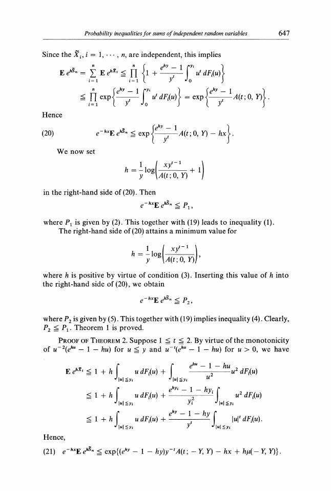
Since the , 1, ..., n, are independent, this implies

(I { ehr--lfi" }u dFi(uE eh" E ehx’ < 1 + yti=1 i=1

i=Q expyt

U dFi(u expyt

Hence

A(t O, Y)}(20) e-hXE ehs" exp yt A(t, O, Y) hx

We now set

h log + 1y A(t; O, Y)

in the right-hand side of (20). Then

e- hXE ehS. <= Pwhere P is given by (2). This together with (19) leads to inequality (1).

The right-hand side of (20) attains a minimum value for

1h log

Y

where h is positive by virtue of condition (3). Inserting this value of h intothe right-hand side of (20), we obtain

e- hXE eh" <= P2,

where P2 is given by (5). This together with (19) implies inequality (4). Clearly,P2 =< P. Theorem 1 is proved.

PROOF OF THEOREM 2. Suppose 1 __< t __< 2. By virtue of the monotonicityof tl-2(ehu 1 hu) for u =< y and u-t(eh" 1 hu) for u > 0, we have

E ehX’<= 1 + h_1 + h_,l__<y

=< 1 + h

Hence,

(21)

ehu 1 hUu2 dFi(u)u dFi(u) +u2

ul<-yi

ehyi 1 hyi u2 dFi(u)u aF,(u) +

ehr 1 hy fl lul’ dF(u).u dFi(u + yt ,I <-r,

e-h’E e" <= exp{(ehr 1 hy)y-’A(t; Y, Y) hx + h#(-Y, Y)}.

648 D. Kh. Fuk and S. V. Nagaev

Setting

1 xyt-(22) h lo + 1

y A(t; Y, Y)

in the right-hand side of(21), we obtain

(23) e-E ehrS" <= P3,

where P3 is given by (7). Inequalities (23) and (19) imply inequality (6).Theorem 2 is proved.

PROOF OF THEOREM 3. We now proceed to the case >= 2. Considerfirst the case where hy <= t, i.e., hy <__ for 1,..., n. We have

E eX’ <= fl,>_, dFi(u) + fI,,,<_,,e" dF(u)

u ehO. dFi(u1 + h.1-,,

udF(u) + -(24) <_ 1 + h udF(u) + -ul_-<y ul_-<y

Hence it follows that, for hy <= t,

(2:5) e-nE en =< exp(1/2 riB2( Y, Y)h2 hx + h#(-K Y)).Suppose now that hy > t. Let us make use of the monotonicity of

u-t(en 1 hu) for u >= t/h. Let be an index such that hy > t. For thiscase, we estimate E en’ as follows (0 =< 0 =< 1)"

e u clFu)E eh’ <-oo

dFi(u) + h-y,

u dFi(u + -/ fty’

ft;"en"-l-hUutdFi(u)+ dF(u) + h u dFi(u) +

fl fl eh:V’--l--hYift:v’eth2 dFi(u) +1 + h u dFi(u + u u’ dFi(uul-<y ul_-<y Yi /h

(26)

u’ dF(u)eth2 u2 dFi(u) + yt< 1 + h ,l<-,,udF(u)+-The right-hand side of (24) is clearly no greater than the right-hand side

of (26) for any positive value of h. Therefore, inequality (26) also holds for thecase where hy N t. Hence, for h > 0, relation (26) and the inequality

(27)

e-hxE es" <= exP{1/2 e’B2( Y, Y)h2 +Chy 1 hy

yt

+ h#(- Y, Y)}

A(t; O, Y) hx

Probability inequalitiesfor sums ofindependent random variables 649

which follows from it, are both valid.

fl(h) 1/2 e’B2( Y,, Y)h2 ahx,

e 1 hyf2(h) A(t;0, Y) flhx,yt

From this and (19) and (27) it follows that

0<<1,

(28) P{S, >= x} _<_ P{X >= y} + exp{f(h) + fz(h) + h/(-Y, Y)}.i=1

Let

(29) h,etB2 Y,, y),

(30) h2 max logY A(t O, Y)

+ 1

(31)

Suppose condition (11) is satisfied, i.e.,

h2 _<h.

Set h h2 and apply inequality (28). Then

f(h2) + f2(h2) + hz/(-Y, Y)- hae’ -B2( Y, Y)h2 x

ehzy- 1 hzyyt

A(t; O, Y) + h2/t(- Y, Y)

(32)eB2( Y, Y)h xz

x

x A(t, O, Y)h2 + h2u(- Y, Y)

(33) <_ fl__

(1-)x-lt(-,Y,Y)+ A(t O-’iT))1-)x-#(-Y,Y) x ox

h2 fl-----h2y 2

(fix It(-Y, Y))h2

(fix (- Y, Y))h2.

Replacing h 2 in (32) and (33) by the expression (30), we arrive at the respectiveexpressions for P4 and P in (8) and (9). Inequalities (12) and (13) then followfrom (28).

Suppose now that h2 h >= t/y. Clearly, f(h) and fz(h) are convexfunctions, f(0)- f2(0)= 0, f(h) attains a minimum value for h---h and

650 D. Kh. Fuk and S. V. Nagaev

fz(h) for h h2 Set h h on the right-hand side of (28). Thus,

Z2X 2

f(hl) -2 etB2( Y, Y)’ f2(hx) < 0,xu(- Y, Y)

(-Y, Y)he,(_ Y, Y)

By virtue of (28), this implies inequality (15).When h < t/y, it is necessary to make use ofthe estimate (25). Theorem 3

is proved.

PROOF OF THEOREM 3’. As in proof of Theorem 3, it is easy to observethat, for any positive h,

Y 1 fE ehx <= 1 + h u dFi(u + - eth2

e- 1 hyfo’+ ytut dFi(u)"

u dF(u)

From this it is apparent that B2(- Y, Y) and p(- Y, Y) may be replaced on theright-hand side of (27) by B2(- oo, Y) and p(- oo, Y), respectively. Repeatingthe proof of Theorem 3, we arrive at the conclusions of Theorem 3’.

PROOF OF THEOREM 4. Starting with (19), we can estimate E ehs". Wehave

E eh2 1 + h f’ f eh" 1- hUu2 dFi(u)u dFg(u) + u2

<= 1 + h u dF(u) +

This implies

ehy 1 hy(34) e-hE eh" <__ exp

y2

Setting

1h -log

Y

u2 dFi(u

B2( o, Y) hx + hlu(-o, Y)}.xy

B2(- , Y)+ 1

in the right-hand side of this last inequality, we obtain the expression forPv given in (17). This together with (19) leads to inequality (16). Theorem 4is proved.

3. Bilateral Inequality

Theorem 5. For 0 < t <_ 1.

(35) P{IS.I x} Z P{IXkl Yk} + P8,k=l

Probability inequalitiesfor sums of independent random var&bles 651

where

(36) {x xP8 =exp ---log

Y Y

xyt-A(t;-r, Y)

+1

(37)

then

xyt- > A(t Y, Y),

(38)

where

P{[S,I x} k P{IXI yu} + P9,k=l

(39) P9 exp{xy y’ y A(ii 7_ , y)

and P9 <= Ps.PROOF. Let

{X if [Xi[ y,Xi=

0 if [Xi[ > Yi,i-- 1,...,n,

Clearly,

P{[S,I-> x} __< P{,, g= S,,} + P{I,] => x}.

Hence, it follows that

(40) P{}S,[ >_ x) <i=1

P{IXil- Yi} -+- e-hXE

We estimate Eehl"l as follows. Let 0 < =< 1. Observe that [u[-l(ehlul- 1)attains its maximum value in the region lul _-< z for lul z. Therefore,

Hence,

(41) e fehr 1hx EehlS,l <= expyt

-A(t; Y, Y)- hx}.

652 D. Kh. Fuk and S. V. Nagaev

Minimizing the right-hand side of (41) with respect to hand taking condition(37) into consideration, we obtain (39). From this and (40) follows in-equality (38). If we replace h in (41) by its value given by (22), then inequality(35) will follow from (36) and (40). Clearly, /99 /98. Theorem 5 is proved.

4. Special Cases

In this section, is to denote either the order of the truncated momentsor the order of finite moments. We introduce the following notation for finiteabsolute moments and variances:

At," E[Xi[ t, Be, DXi.i=1 i=l

Observe that the proofs of Theorems 1-5 remain valid if in inequalities(20), (21), (27), (34) and (41) the truncated absolute moments and variancesare replaced by the full absolute moments and variances, respectively. Hence,under the assumption that the absolute moments of any order exist, onecan replace the truncated absolute moments in the various inequalitiesobtained in Theorems 1-5 by the full absolute moments.

We shall now state some consequences of Theorems 3 and 4.Suppose first that the i.r.v. X, ..., X, satisfy the following conditions:

(42) X I.,i, EX O, 1,’.., n.

Let Yi Li, i= 1,-..,n, and let y L max{L,.-.,L,}. ThenTheorem 4 implies

Corollary 1. Suppose the i.r.v. X, X, satisfy conditions (42). Then

(43) P{S >_ x} __< exp -+LIlog + 1

We point out that inequality (43) was obtained independently byBennett [10], [11] and Hoeffding [12],

Let t/(t ./ 2) and e 1- ft. Then inequalities (13) and (15) ofTheorem 3 imply

Corollary 2. Suppose t >= 2, fl t/(t + 2) and 1 ft. Then

(44) P{S, >_ x} __<i:

P{XiYi}+ exp{maxl- x /2(- Y, Y)

Y Y

flxy’-x log .Ai[ )) + 1 ,- x(x/2-1(-Y,Y))]}etB2(_ Y, Y)

(45) <--i:1

P{Xi>=Yi} + exp {-- flx-y P(-Y’Y)Ylog

A(t O, Y)+ 1 + exp

etB2(_ Y, Y)

Probability inequalitiesfor sums ofindependent random variables 653

From Theorem 3’ follows

Corollary 3. Suppose t >= 2, fl t/(t + 2) and 1 ft. Supposefurtherthat EX O, 1,..., n. Then

(46) P{S,_>x}_< P{X,y,} +exp max _fiX_log + 1i= y A(t; 0, Y)

(47)i=1

P{X, > y,} +A(t’O, ) + 1

x/y

+ exp {-Set y

obtainy //x in (46) and (47). Then from Corollary 3 we

Corollary 4. Let EX 0 and EI Xi[ < , 1,..., n, for t : 2. Then

(48) P{S, x} cll)At,nx-t + exp{-c)xZ/B2,},where cl)= (1 + 2/0’ and c12)= 2(t + 2) -1 e -t.

5. Examples

In this section, we shall give some examples involving the calculationof probabilities on the basis of the resultant inequalities. The set of n positivenumbers y will be chosen in arbitrary fashion. When x is large, this permitsus to select y so that both components on the right-hand sides of theseinequalities have small values simultaneously. Some specific examples arecited and they are compared with the inequalities obtained earlier by otherauthors ([5], [9]-[12).

We shall consider the case where the moments of order 0 < _< 2 exist.To make things convenient while computing the probabilities, we shall assignvalues to x and y of the form x aA,,, and y bA,,,, where a and b arepositive numbers. To simplify notation, we shall omit writing the subscriptson At,n

1. Case 0 < t < 1. It follows from inequality (35) that

(49) P{IS.I >_- x} =< P{IXi[ >_- y,} + eo,i=1

where

logPo expyt y

We wish to show that for 7 => 1 and X > 7e2A, it is possible to choosey so that the relation

(50) PlO < Ax-t/7is satisfied.

654 D. Kh. Fuk and S. V. Nagaev

For, suppose 0 < 2y =< x. Let z A/xy- and x/y c. Observe that0 < ze-z =< 1 for all z > 0. Therefore, under the given conditions we have

Po (ze-Z) <= (ez) (eAc’-Xx-t)z < Ax-’. eZAx -’ <=The familiar Chebyshev inequality yields the bilateral estimate

(51) P{IS.I >_- x} __< Ax-’.

In the next example we compare the estimates (49) and (51). SupposeX,..., X, are i.r.v, with common Cauchy distribution function on thepositive real line, namely,

F(u) u > 0n 1 +z2’

For definiteness, take t 2/3 and n 2 and 8. The first table furnishesvalues of the right-hand sides of inequalities (49) and (51).

2. Case 1 _< t =< 2. For identically distributed i.r.v., Bengt and Esseen[9] obtained the following bilateral estimate"

(52) P{IS.] >= x} =< M(t, n)Ax-’,

where

M(t, n) I min{2 n

(53) 2 n-- [1 -D(t)] } forD(t)

13 52F(t) sintTtzt(2, 6)’ 2

otherwise.

x y (49) (49)A3/2 A3/2 (51)

n 2 n 8

2 1 .6300 5523 .33386 a .3299 .1383 .085210 2 .2154 .0819 .0422

.1721 .0504 .02781418 1456 .0381 .020524 6 .1201 .0278 .0145

(54)

For symmetrically distributed summands, Theorem 2 gives

P{S, => x} __< P{X >= y,} + Pll,i=1

where

(55)

P =exp + logxyt-A

+1

When x > 97e2A, 7 _>- 1 and 1 =< t =< 2, the following relation holds"

Pll < A(xt + A)-1/7 < Ax-t/y.

Probability inequalitiesfor sums ofindependent random variables 655

Indeed, suppose 2 .<_ x/y c <= 3 and z A/xyt- . We have

P [e(1 + 1/z)--]c< ]2 < + A)-9AeZx-tA(xl+z

<= A(x’ + A)-1/3) < Ax-t/y.

Taking (55) into account, one can hope to obtain, for large x, betterestimates than those given by inequality (52) and Cantelli’s inequality

(56) P{S, >__ x} _<xz +

by choosing the values of y in inequality (54) suitably.Let X, ..., X, be i.r.v, with common distribution function F(u)

1/2(1 + u(1 + u)-a/2). It is not too hard to see that X1, ..., X, are sym-metrically distributed, DX oe and EIX[ < oe for 0 < t < 2. Chooset 9/5 and n 2 or 10 (for t 9/5, M(t, n) 1.285 in (53)). We obtain thefollowing table of values for the right-hand sides of (52) and (54):

x (54) (54)A/-- A5/9 (52)

n 2 n 10

.36903 .29552 .289992 34 .10598 .04548 .050068 3 .03043 .00763 .0068914 6 .01111 .00177 .0016122 9 .00493 .00048 .00047

We now give one further example demonstrating the accuracy of theestimates (54) and (56). Let X, ..., X, be i.r.v, with common distributionfunction

2 f" dzV(u)

rt (1 + z2)2

It is not hard to see that EX1 0 and DX1 1. We have the followingtable"

(54) (54)x y(56)

B. B. n 4 n 16

2 .20000 .35474 .330584 .05882 .06533 .049498 3 .01538 .00424 .0037212 5 .00689 .00129 .0009116 6 .00389 .00052 .0003824 12 .00173 .00009 .00004

656 D. Kh. Fuk and S. V. Nagaev

As Hoeffding pointed out in [12], inequality (43) refines the followinginequality due to Yu. V. Prokhorov 5]:

P{S >- x} __< exp2L

arcsin

As Yu. V. Prokhorov pointed out, this estimate improves the inequality ofS. N. Bernstein and A. N. Kolmogorov. Inequality (43) also refines thefamiliar Cantelli inequality (56).

6. Applications to the Strong Law of Large Numbers

Let

(57) x, 2, ,,be a sequence of symmetrically distributed independent random variables.It is known that it does not restrict the generality if one requires symmetrywhen studying conditions for the applicability of the strong law of largenumbers (see 2], [3]). Suppose that the variables in the sequence (57) arecentered about their means, i.e., E 0 for all k >__ 1.

We partition the sequence into classes by including in the r-th class therandom variables with k I {2",2 + 1,-.., 2+ 1}, r >= 0.

Let {6} be a sequence of positive numbers. Introduce the followingnotation (the summation is everywhere with respect to k e I)"

Z, 2-’, K(t, 6, r) 2-’" u’ dF(u),"0

(58)

H((r, r) E 2-2r J_ U2 dFk(U), Hr E 2-2Dk.2"6,.

The following condition (due to Yu. V. Prokhorov 2])"

(59) Z P{Z, >- e} < oo, V e > 0

is necessary and sufficient for the sequence (57) to obey the strong law oflarge numbers, i.e., for

n-({ +...+ {,)--+0 a.e.

For t >= 2, inequality (45) leads to

(60)

where e et(t + 2)-1 and 32 2g2e-t(t + 2) -2.

Probability inequalitiesfor sums of independent random variables 657

It is not hard to see that if the series

r---1

and exp{-e/H(,r)}r=l

are convergent for all positive e, then the series obtained by replacing e and;2 by e are also convergent for all positive e, and conversely. Therefore,when using condition (59), we can substitute e for e and 2 on the right-hand side of (60). Thus, we have

Theorem 6. Let {6} be a sequence of positive numbers such that the fol-lowing conditions hold for any positive e"

(61)kIr

(62) (e6 /K(r, 6, r) + 1) -/r < oe, t >__ 2,r--1

(63) exp{-e/H(6, r)} < oe.r=l

Then the sequence (57) obeys the strong law of large numbers.

RhlI 1. Denote H(6,, r) by q,. Then for t 2, condition (62) can berewritten in the following form"

From this we see that if q),--, 0 as r , then (62) implies (63). But iflim inf,_oo q), > 0, then (62) and (63) are equivalent.

If the absolute moments of order t => 2 exist, then the following theoremis valid.

Theorem 6’. Suppose the sequence (57)is such that Elkl < oc for >= 2and for all k >= 1. Then the fulfillment of condition (61) and the following con-ditions"

(64) (6’- /Kt, + 1)- /" < oe,r=l

(65) e-m" < oe, V e > 0,

where K,,, and H are given by (58), is sufficient for the strong law of largenumbers.

We state now some corollaries to Theorem 6’. Setting 6, e/- / > 1we obtain

658 D. Kh. Fuk and S. V. Nagaev

Corollary 1. If t >= 2 and there exists a constant fl >= 1 such that for anypositive conditions (65) and

(66)k=l

(67)r=l

hold, then the sequence (57) obeys the strong law of large numbers.It is well-known that condition (66) is necessary for the strong law of

large numbers.

Corollary 2. If condition (66) holds and there exists a fl >_ 1 such that

(68)r--1

then the strong law of large numbers holds.

REMARK 2. Let {b,} be a non-decreasing sequence of positive numberswith b, .

V. A. Egorov 7] showed recently that if

m 2grn 2 2 < oo k > 2,(69) P([,[ > b,) < and -a...a_,= n U

where aj2---D{j and the inner summation extends over all j, j_satisfying 1 < j < < j_ < n 1, then (b,)-1 , j 0 a.e.

It is interesting to compare conditions (68) and (69) when b, n.We first give an example to show that generally speaking (68) does not

follow from (69).2 2 if n n and vanishes forFor, let n j2J= j)/2 and assume a,

other values of n. It is not hard to see that

j--2 )2(j-a, <(j-l_

n=l

Hence, the sum of the series occurring in condition (69) does not exceed2=j a for k 2. At the same time, 2 2a,Jn as j m from whichit follows that condition (68) cannot be satisfied no matter what fl >_ 1.

variesIn this example, the sequence {a,2} contains large gaps. But if a,regularly as n m, then the case when lim,_BZz+,/B. < c with

n--n /--n

2B,2 i= /2 and, in addition, lim inf,_ ltk)/l2k > 0, where Bt,k) Za2 (the summation being over thosej, "’’,Jk which satisfy 1 <= j <

< Jk < n) is typical. In that event.

ZHk Z2-a"Z a,H2 k--1

nlr

2 2k- 2o’B< L1 Y=I r/2k

oo 2 (k-l)6nBn< L2 Y=I /2k

Probability inequalitiesfor sums ofindependent random variables 659

where L and L2 are constants, or in other words, from condition (69) followscondition (68).

Setting fl 1 in (67) and using Chebyshev’s inequality, we arrive at

Corollary 3. Condition (65) and the condition

(70)kt

< , t > 2,k=l

are sufficient for the strong law of large numbers.

RhgK 3. When t => 2, Yu. V. Prokhorov 2] (and Brunk [8] for even t)showed that the condition

(71) k,/ + - < ck=l

is sufficient for the strong law of large numbers. Since

nl. nlr

condition (71) implies conditions (.65) and (70) under which Corollary 3 isvalid.

as k . Then theCorollary 4. Let O(k/qg(k)), where qg(k) Tcondition

(72) (e/qg(2r)Kt,r + 1) -2") < o, V e > 0, t >_ 2,r=l

is sufficient for the strong law of large numbers.

REMARK 4. Yu. V. Prokhorov proved in [4] that the condition

(73) e-/m < , V e > 0

is necessary and sufficient for the strong law oflarge numbers if (k) loglogk.We can show that in this case condition (72) is necessary and sufficient forall t 2. To this end, we merely have to prove that (72) follows from (73)for t 2, since

Kt, K(t, 1, r) H(1, r)= H,if,<n, VnI.

Without loss of generality, we may assume that (2) log r. Setg 1/log r. If eg/H e2/ 1, then

(e6,/H, + 1) -/" r-2.

But if 86r/Hr < e2/a- 1, then the inequality log(x + 1) x/(x + 1)leads to

(el6,) log(e6,/H, + 1) > e,Ze-Z/e/Hr.

660 D. Kh. Fuk and S. V. Nagaev

Thus

Z (e6,./H, + 1)-/a" < Z r-2 + Z exp{-e2e-2//H,}r=l r=l r=l

REMARK 5. Under conditions (67) and (68), Kt,, and H, may be replaced,respectively, by K(t, 1, r) and H(1, r) since there is no loss of generality inassuming that [,l < n.

Received by the editorsSeptember 3, 1970

REFERENCES

[1 S. V. NAGAEV, Some limit theorems for large deviations, Theory Prob. Applications, 10(1965), pp. 214-235.

[2 Yu. V. PgOKHOROV, On the strong law oflarge numbers, Izv. Akad. Nauk SSSR, Ser. Mat.,14, 6 (1960), pp. 523-536. (In Russian.)

[3] Yu. V. PROKHOROV, Strong stability of sums and infinitely divisible distributions, TheoryProb. Applications, 3 (1958), pp. 141-153.

[4] Yu. V. PROKHOROV, Some remarks on the strong law oflarge numbers, Theory Prob. Applica-tions, 4 (1959), pp. 204-208.

[5] Yu. V. PgOKHOROV, An extremal problem in probability theory, Theory Prob. Applications,4 (1959), pp. 201-203.

[6] A. BIKYALIS, Estimatesfor the remainder term in the central limit theorem, Litovsk. Mat. Sb.,6, 3 (1966), pp. 321-346. (In Russian.)

[7] V. A. EGOROV, On the strong law of la’ge numbers and the law of the iterated logarithm fora sequence of independent random variables, Theory Prob. Applications, 15 (1970),pp. 509-514.

[8] H. D. BRUNK, The strong law of large numbers, Duke Math. J., 15 (1948), pp. 181-195.[9] V. B. BFNGT and C. G. ESSEEN, Inequalitiesfor the r-th moment ofa sum ofrandom variables,

__< r __< 2, Ann. Math. Statist., 36, (1965), pp. 299-303.[10] G. BENNETT, Probability inequalities for sums of independent random variables, J. Amer.

Statist. Assoc., 57, 297 (1962), pp. 33-45.[11] G. BENNETT, On the probability of large deviation for the expectation for sums of bounded

independent random variables, Biometrika, 50, 3 (1963), pp. 528-535.[12] W. HOEFFDING, Probability inequalities for sums of bounded random variables, J. Amer.

Statist. Assoc., 58, 301 (1963), pp. 13-30.