Materiel Test Procedure 5-2-529O 7 December 1967 White Sands Missile Range

U. S. ARMY TEST AND EVALUATION COMMANDCOMMON ENGINEERING TEST PROCEDURE

RADAR RECEIVERS

1. OBJECTIVE

"I• The objective of this procedure is to measure and compare with specifiedvalues the characteristics of a radar receiver.

2. BACKGROUND

The performance characteristics of a radar receiver are usually deter-mined by its ability to acquire, track, discriminate, and display targetsaccurately. The parameters of the individual components and effects on them ofinputs other than the basic signal information, (i.e., noise), are amongthe limiting and determining criteria for the performance functions.

3. REQUIRED EQUIPMENT

a. FM Sweep Signal Generatorb. Directional Couplerc. Terminating impedancesd. Oscilloscope or A-scopee. CW Generatorf. (O-lma) Milliammeterg. Argon Gas tube generator and mounth. Variable Attenuatori. Microwave Power Meterj. Marker Oscillatork. Test Power Supply (for bench tests)1. Waveguides, connectors, and cables appropriate to the test and

the receiver.m. Data Sheets and Graph Papern. Desk calculatoro. Standard Math Tablesp. Noise Figure Meter (if available)

4. REFERENCES

A. Henney, Keith, Radio Engineering Handbook, McGraw-Hill, New York,1959.

B. Electronic Precision Measurement Techniques and Experiments, Staffof Philco Technological Center, Prentice-Hall, New Jersey, 1964.

C. Microwave Power Measurement, Hewlett-Packard Application Note 64,Hewlett-Packard Company, 1965.

D. Noise Figure Primer, Hewlett-Packard Application Note 57, Hewlett-Packard Company, 1965.

E. Principles of Radar, MIT Radar School Staff, McGrawHill, New York1946.

F. Radar System Measurements, Philco-Ford Corporation, Techrep Division,1966.

-1-

.a.uo y o .y o3

S $

MTP 5-2-5297 December 1967 0

G. Skolnik, Merrill I.., Introduction to Radar Systems, McGraw-Hill,1962.

H. Swept Frequency Techniques. Hewlett-Packard Application Note 65,Hewlett-Packard Co., 1965.

I. Terman, Fredrick E., Electronic and Radio Engineering, McGraw-Hill,1955.

5. SCOPE

5.1 SUMMARY

Radar receiver performance is determined by a great many factors mostof which are established in the original design. The ones which are usuallyconsidered to be the most important and which will be considered in this testare:

a. Receiver sensitivityb. Receiver noise figurec. Receiver bandwidthd. Receiver recovery

In many radar systems, circuits are included for special functions.Four common circuits are:

a. MNTI (moving target indication) 0b. IAGC (instantaneous automatic gain control)c. STC (sensitivity time control)d. FTC (fast time constant)

These circuits may be found in combination or singly depending uponthe purpose of the radar. In the radar testing procedures to be described, thespecial functions should be disabled. If an automatic-frequency-control circuit(a.f.c.) is included in the radar, it may be left on during receiver tests.A good check on a.f.c. is to make the tests specified for manual tuning; thenswitch to a.f.c. If the a-f-c circuit is normal, the signal indications shouldnot change. The tests are summarized as follows:

a. Receiver Sensitivity: Determines the ability of the radar topick up weak signals. The greater the sensitivity, the weaker the signalthat can be picked up. Sensitivity is measured by determining the power levelof the minimum discernible signal (MDS).

b. Receiver Noise Figure: The noise figure is used to indicate howmuch noise is to be expected. It is defined as the ratio of measured noise tocalculated noise, and may be expressed as a power ratio or in db. The noisefigure is determined by the use of either a noise generator or a C-W signalgenerator.

c. Receiver bandwidth: The test determines the frequency spreadbetween the half power points on the receiver response curve.

d. Receiver Recovery Time: This test determines the time requiredfor the receiver sensitivity to return to normal after a saturating echo isreceived.

-2-

MTP 5-2-529Q 7 December 1967

5.2 LIMITATIONS

The procedures contained in this MTP are intentionally general toprovide information for measuring the critical functions of various types ofradar receivers. Because of the scope and complexity of the equipment, it isnot possible to include all of the details required to test receivers. Thereader should consult the references listed in this NTP for additional datathat will aid in conducting tests of radar receivers. All tests areto be conducted at room ambient temperature. Environmental tests are notwithin the scope of this MTP and may be investigated by the use of other MTP'sor appropriate Military Specifications.

6. PROCEDURES

6.1 PREPARATION FOR TEST

The complete technical description of the receiver under considera-tion should be on hand. This should include all schematics, drawings,specifications, manuals, and the results of previous checkout and/or acceptancetests if possible.

These documents should be reviewed with regard to the equipmentoperating limitations to prevent overloading or otherwise damaging the equipment.

0 The safety criteria as specified in the documentation should also beconsidered.

Personnel conducting the test should be familiar with radar and radiooperating and test procedures. The receiver to be tested should be in goodrepair with all required maintenance operations having been previously performed.

6.1.1 Special Procedures and Equipment

The following conditions and precautions hold throughout the tests.

a. Signal generators must be impedance matched to the receiver sectionfor which they are supplying signal power. Mismatches will cause reflectionswhich will result in standing waves and erroneous readings. Tuning stubs shouldbe inserted in the RF line (cable or waveguide) to obtain an impedance match.Tuning stubs-will'only work for sinusoidal signals. Pulse or digital signalsrequire that the characteristic impedances of the receiver, transmitter, andline be equal.

b. The signal generator's output level must be such that it will notoverdrive or cause distortions in the receiver component's output.

c. In order to'prevent excessive energy losses, spurious responses,interference patterns from being set up, and extraneous noise from being intro-duced into the system, all connections should be tightly and rigidly madeand shielded cables should be used whenever possible.

d. To minimize power losses, wave form distortion, and time delaysunshielded leads should be kept as short as possible.

-3-

MTP 5-2-5297 December 1967

6.2 TEST CONDUCT

6.2.1 Receiver Sensitivity

An receiver sensitivity measurement is essentially an minimum discerrnblesignal (MDS) test. An MDS measurement consists of measuring the power levelof a pulse whose level is just sufficient to produce a visible receiver output.The output of the receiver is to be taken with an A-scope. A conventionaloscilloscope may be utilized as an A-scope if the receiver does not have anA-scope display.

The procedure for making an MDS measurement, using an FM signalgenerator is as follows: (see Figure 1.)

a. Connect radar trigger-pulse output to trigger-input jack onFM signal generator. (Omit if interval sync is desired).

b. Connect r-f input through coupling device to radar. (A directionalcoupler is preferred).

c. Turn signal-width control to maximum (CW).d. Adjust phase control for maximum Klystron output as indicated on

thermistor bridge.e. Tune Klystron (cavity) to approximate radar frequency, by adjusting

the frequency meter to the frequency of the radar transmitter and tuning theKlystron for a dip in the thermistor-bridge meter reading. (Since the Klystronmode is fairly broad, extreme accuracy in tuning the Klystron is not necessary.For example, the width of the flat portion of an X-band Klystron is about 10 MHz;therefore, the tuning accuracy required is ±5 MHz.

f. If necessary, adjust phase control again for maximum output. Ifa large adjustment is required, repeat step 5 again.

g. Adjust uncalibrated attenuator for a 1-mw indication.h. Set receiver gain control for a 1/41" noise level on the A-scope.

(This will have to be done at a low setting on the calibrated-attenuator control.)i. If necessary, adjust phase control to position echo pulse in a

target-free area.j. Adjust signal-width control for desired echo-pulse width.k. Set calibrated attenuator until echo is just barely visible in

the noise. This is the MDS level. (Rock phase control during this step tomake the echo more easily visible.)

1. Record the attenuator setting, the loss in the coupler andthe cabling losses. The coupler and cabling losses must be known prior tostarting the test.

m. To eliminate the possibility of signal leakage giving erroneousreadings all equipment associated with MDS tests should be located outsidethe radar-antenna radiation field. In addition, the equipment should neverbe operated outside of its case, or with loose cable connections.

6.2.2 Receiver Noise Figure

A knowledge of the noise figure of an operating radar receiver isalso important as a measure of receiver sensitivity. The larger the noise

-4-

MTP 5-2-5290 7 December 1967

EXTERNAL SYNCI

*SWEEP, U-F ATTENATOR ATTEURAlOR IIOPEIGainE- OSCILLATCH (UNCAUb1 (0*1.2-

-ASR *ATED) MRATED)

I DT

IIENLDIM I

I SECOND

IDETECTORK) A SCOPE O

OSILOSOP

Figre1.Equpmntcoecio forNA G NESReAsremnt

Figre . pperane f MS masremnt n -scpe

OU5- O

NTP 5-2-5297 December 1967 Q

figure, the poorer the sensitivity. There are two basic methods of measuringnoise figure. One method utilizes a CW signal generator and the other uses aknown source of broad band noise power, such as an argon-gas tube.

6.2.2.1 Noise Figure Measurement With.aCW. Signal Generator

This method of measurement has the advantage that it can measurethe noise figure over a wide range of value; however, the receiver noisebandwidth must be known. -This bandwidth is not the 3-db or .707.bandwidthand its measurement would involve a complete knowledge of the responsecharacteristics of the receiver. The frequency response characteristics ofpractical radar receivers are such that the 3-db and the noise bandwidths donot differ appreciably. Therefore, the 3-db bandwidth may be used as anapproximation to the noise bandwidth. The test is conducted as follows.

a. Connect a milliammeter (O-lma.) in series with the diode loadof the radar-receivers second detector.

b. Adjust the receiver gain to give a .5 ma. reading. (This readingis due to noise alone.)

c. Connect the CW signal generator to the receiver input. (Figure 3)d. Tune the CW signal generator to the center of the receiverts

bandpass characteristic. (3-db characteristic for most receivers)e. Raise output of CW generator until meter reads .707 ma. (1.4 X .5).

(At this point make sure that a further increase in noise causes a correspondingincrease in meter reading. If not, the receiver is limiting and the readings C)will not be accurate. In this case, use a lower current in step b; for example,start with .3 ma. and raise to .42 ma. in step e.)

f. The CW generator power output is now equal to the receiver noise

power. Note the generator amplitude dial reading. (A chart is usually furnishedfor converting dial readings to power.) /

SCALIBRATED I 'RECEIVER UNDER MILOUTPT OF ,'

SCW GENERATOR -! TEST. 2ND DETECTOR MLAMTR

Figure 3. Test Setup for Noise Figure Measurement with a CWGenerator

6.2.2.1 Noise Figure Measurement with a Gas Tube Noise Generator

The procedure is the same as with the CW generator except that thegas tube noise generator as shown in Figure 4.,, nom replaces the CW generator.

The method is generally preferable to the use of a CW generatorbecause the noise bandwidth of the receiver does not have to be known and themeasurements are simplier and are more reproducible. Noise figure measurementsmade with the signal generator method may not always agree with measurementsmade with the noise-source method when nonlinear networks such as mixers or

e"* - . . .- 6-

MTP 5-2-5290 7 December 1967

INPUT TERMINATION

Figure 4. Diagram of a typical Gas Tube Generator

parametric amplifiers are involved. Caution should be exercised in the inter-pretation of such measurements. An ordinary superheterodyne receiver-respondsequally well to the image frequency as to the signal frequency. Therefore,when a broadband noise source covering both the image and the signal bandsis used to measure noise figure, the effective receiver bandwidth is twice thenoise bandwidth, but it is only the noise bandwidth in the signal generatorcase. The noise figure as measured with the broadband noise source will be3 db lower than that with the signal generator case. When an image-rejectionfilter is used at the radar input, the two methods agree. If. no filter is used,the receiver will be equally sensitive to both the image and the signal, andmeasurements made with the broadband noise source should be increased by 3 dbto obtain the'valid noise figure.

The power output of the noise generator is usually controlled bya variable attenuator which is calibrated to read noise figure directly by thefollowing procedure.

a. Connect the gas tube noise source to a variable attenuator andin turn to a standard power meter.

-b. With the noise source turned off and the attenuator turned tominimum attenuation setting the power meter to a 1mw level.

c. Fire, the noise generator with the attenuator setting the same andnote the power meter reading.

d. Repeat b and c for ten attenuator settings from minimum-throughmaximum attenuation.

e. Record the attenuator settings and the power readings.

The techniques described are quite similar. Variations of thesemethods are employed, but the basic principles are the same. Examples ofthese tests are foiud in MTP 5-2-510 "Noise Tests of Guidance Components".

-7-

0 3

MTP 5-2-5297 December 1967

SNOISE SCOURGE A ..... . TTENUATOR " Ii.." POWER METER ...

Figure 5. Connection of Equipment for Attenuator Calibration.

There are commercial noise figure meters available whose use is well spelledout in the instrument's instruction manuals and may be utilized if available.These meters indicate noise figure directly and depend on the periodic insertionof known excess noise into the system. This results in a pulse train of twopulse levels, N2 and N1 . The pulse train'typically is amplified in an IFstrip and then-separated into two distinct levels by selective gating. Theselevels, together with the amount of excess noise insertion, contain the CJinformation needed to directly indicate the noise figure on a meter face.Such an instrument is shown in simplified block diagram form in Figure 6.

6.2.3 Receiver Bandwidth

Receiver bandwidth is the frequency spread between the half-powerpoints on the receiver response curve. Figure 7 shows a typical response curve.Since this curve is in terms of voltage, the half-power points are representedby the 70.7% voltage points (ýFT/ = .707).

The method for measuring bandwidth used the same setup as for DS.measurements using the FM signal generator. The measurement procedure is asfollows:

a. With the equipment connected in the same manner as for an MDS

measurement, turn the signal-width control to obtain a response curve about.one half inch wide.

b. Reduce receiver gain to obtain a noise amplitude that is -justbarely visible.

c. Adjust calibrated attenuator to produce a pulse amplitude below-receiver saturation level.

d. Tune frequency meter until response curve shows an absorption pipat one of the half-power points.

e. Read the frequency, then repeat for the other half-power point.The difference between these two frequencies is the receiver bandwidth.

-8-

MTP 5-2-5297 December 1967

4

(D~~~~~~~~~~~~A Fiur 6.SmlfeFlc igrmo uoai os

fiue esueet sytm

AII~ftIF1ER

Whgen the foegingpriidbocdr disga used thalf-o weri poinse myb

located very easily as follows:

a. Note the attenuator dial reading following step c. above.b. Increase the reading 3db and mark the level at the top of the

response curve.c. Return the attenuator to the previous value.d. The half-power is at the level marked in step b.

The bandwidth measurement procedure given above is used when thereceiver is operating as a part of a radar system. When the radar receiver isto be tested as an individual component, the following method is used. Figure8. shows the test setup for checking a receiver separate from the radar system.

a. Connect a sweep generator to the receiver 1-f input. (The rangeof frequency of an FM signal generator and the center frequency of the sweep isusually adjustable to cover any standard radar i .f.)

*b. Feed-the receiver video output to the vertical-deflection c4.rcuit

-. c. Connect the synchronizing voltage of the sweep generatort ,external synlc terminal of the oscilloscope. The oscilloscope now indicatesg

-9- L

L•DETECTOR

MTP .5-2-5297 December 1967

frequency horizontally and receiver output vertically.d. A second signal generator, called the marker oscillator, produces

an accurately calibrated C-W signal which is mixed with the sweep-generatoroutput.

e. The sweep-generator as it nears the marker-oscillator frequency,produces a marker pip on the response curve as shown in Figure 9. The markeroscillator dial will indicate the frequency at which the pip occurs.

f. Change the frequency of the marker oscillator until the pip is atthe 70.7% on the curve. Read the marker oscillator dial.

g. Move the pip to the other 70.7% point. Read the marker oscillatordial.

., RECEIVER BANDWIDTH

70.70% 3D9

a..

" FREQUENCY " ""

Figure 7. Frequency Response Curve.

I F IN PUT "VIDEO'OUTPUT

SIGNA RKE RADA OSCTEST

TES

PWROSC SUPPLY

tSYNC SIGNAL C

Figure 8. Receiver Response ,.Test Setup.

-10-

MTP 5-2-5290 7 December 1967

MARKER PIP(FREQUENCY

INDICATION)

a.

0

FREQUENCY

Figure 9. Indication Obtained with the Test Setup shown in Figure 6.

6.2_4 Receiver Recovery Time

Radar receiver recovery time is defined as the time required for thereceiver sensitivity to return to normal after a saturating echo is received.

a. Use the same test setup as for an NDS measurement.b. Set receiver gain to give about 1/8" noise on A scope.c. Adjust the attenuator to give a pulse amplitude that will saturate

the receiver.d. By use of the calibrated time base on the A scope determine the

time required for the noise to return to its original level as indicated byFigure 10.

SATURATING ECHO

"RECEIVER RECOVERY PERIOD

Figure 10. Receiver Recovery using a Saturating Echo.

-11

MTP 5-2-5297 December 1i967

6.3 TEST DATA

6.3.1 Receiver Sensitivity

Record the following:

a. The attenuator setting in db.b. The cable losses in db.c. The coupling loss in db.d. The nomenclature of the receiver.e. The serial number of the receiver.

6.3.2 Receiver Noise Figure

Record the following:

a. CW Generator Method'

1) The attenuator setting in mW2) The nomenclature of the receiver3) The serial number of the receiver

b. Noise Generator Method

1) The attenuator setting in units or db as appropriate C)2) Calibration technique

a) Record attenuator setting (units)'and power readings (mW).

6.3.3 Receiver Bandwidth

a. Record receiver data as before.b. Record in MHz the frequencies corresponding to the half power points.c. Record in MHz the marker oscillator dial readings at the half

power points.

6.3.4 Receiver Recovery Time

a. Record Receiver data as beforeb. Record the-measured recovery time in ý sec.

6.4 DATA REDUCTION"

6.4.1 Receiver Sensitivity

Find the total attenuation in db. The value obtained is the MDS indb below imw. (-dbm)

Total attenuation = coupling loss (db) + cable loss (db) + attenuatorreading (db). Compare to the value specified for the receiver.

-12-

MTP 5-2-5297 December 1967

6.4.2 Receiver Noise Figure

a. CW generator method

Calculate the noise figure by means of one of the followingformulas:

P measured-NF = P calculated

P measuredNF(db) = 10 log P calculated

where: NF = noise figureP measured =attenuator setting in, mWP calculated = KT A F

K = Botzmann's constant 1.38 X 10-•3 joules per degree Kelvin-T = Temperature in degrees absolute. (Kelvin Scale)

Usually 290°K'A F = Range of frequencies involved (bandwidth) in MHz.

b. Noise generator method

The noise figure of a receiver which is being supplied by a gastube noise generator can be shown to be:6> (T 2 -To) 1

:NF= TO X (1i)

N,

where: F = noise figureTo = room temperature of 290°KT2 = the equivalent absolute temperature of the noise source

(10.O00° 0 K for a Argon Gas Tube).-N = noise power out of attenuator with tube on. (power meter

reading in MW)N, = noise power out of attenuator with the tube off. (power

meter reading 1MW in this test)

Converting to logarithmic notation(T2 - TO) (N 2 1)

Fdb = 10 log To -10 log N1

The ratio (T2 - To)/To is a measure of the relative excess noise.power available from a noise source and is specified by the manufacturer. Inthe case of argon gas tubes, thisratio is 33:1; 10 log (T2 - To)/To is 15.2ab. When using such a tube, the equation simplifies to:

Fdb =.15.2 - 10 log (N./Dý - 1)

Since the ratio N2 /IN can be determined at each attenuator setting~ taken the noise figure can also be determined at each point. A graph of noise

-13-

MTP .5-2-;529"7 December 1967 ( "

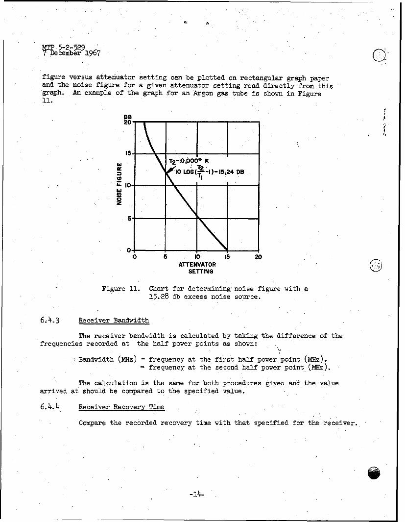
figure versus atteniuator setting can be plotted on rectangular graph paperand the noise figure for a given attenuator setting read directly from thisgraph. An example of the graph for an Argon gas tube is shown in Figure11.

DB e.20

15.T2-Ioo0oo K

10 L 11(-15i24 DBaI0.

io

0z

5.

0'0 5 to 15 20

ATTENVATORSETTING

Figure 11. Chart for determining noise figure with a15.28 db excess noise source.

6.4.3 Receiver Bandwidth

The receiver bandwidth is calculated by taking the difference of thefrequencies recorded at the half power points as shown:

...Bandwidth (MHz) = frequency at the first half power point (MHz).= frequency at the second half power point (MHz).

"The calculation is the same for both procedures given and the value

arrived at should be compared to the specified value.

6.4.4 Receiver Recovery Time

Compare the recorded recovery time with that specified for the receiver.

-14-