THE DESIGN AND CALIBRATION OF A

VISCOUS AIR FLOW METER

By

S. VICAR HUSAIN 11

Bachelor of Science

Nizam College

Hyderabad., India

1947

Bachelor of Engineering

Osmania University

Hyderabad, India

1949

Submitted to the Faculty of the Graduate School of

the Oklahoma Agricultural and Mechanical College

in Partial Fulfillment of the Requirements

for the Degree of

MASTER OF SCIENCE

1955

THE DESIGN AND CALIBRATION OF A

VISCOUS AIR FLOW METER

TtlESIS APPROVEDi

Thesis Adviser

Dean of the Graduate School

ii

PREFACE

Engineers who deal with research and development work on

machines through which there is air flow are ever conscious of the

need for improved devices for measuring air flow - particularily in

cases where the flow is not steady. Thus the inadequacy of existing

equipment present a challenge to the individual to improve existing

designs or develop new and improved designs.

The need for an improved device for measuring the air flow to

an internal combustion engine prompted the author to design and cali­

brate the viscous air-flow meter dealt with in this report.

Throughout the report it is assumed that the reader is familiar

with the fundamentals of hydraulics as applied to flow problems. The

entire report can be of value to those who are concerned with air

flow measurement under pulsating or steady flow conditions. The

author now wishes to express his sincere thanks to Professor W. H.

Easton for carefully reading the entire report and offering valuable

suggestions and comments, and to Professor B. S. Davenport for his

valuable advice and practical suggestions. I also wish to express

my special appreciation and thanks to Professor Gordon Smith for his

valuable help in machining the nozzles and other pieces of apparatus

used during the test.

iii

TABLE OF CONTENTS

Chapter Page

I. INTRODUCTION • o • • • • • • • • • • • • • • • • • • • • • 1

II. REVIEW OF LITERATURE • • • • • • • • • • • • • • • • • • • 3

III. STATEMENT OF PROBLEM e O O O • e • 0 0 • 0 0 0 0 O O O e • 10

IV. ANALYSIS OF THE PROBLEM AND THEORY oe•o••oo•••• 11

Theory of Viscous Flow •• 0 0 0 OO<tOoO•••oo 12

Viscous Flow in Capillary Tubes. oeoooooeoo 15

V. THE DESIGN OF THE VISCOUS FLOW ELEMENT • • ooooec:ioo 22

VI. DESCRIPTION OF THE APPARATUS AND EQUIPMENT •••••••• 29

Filtering Element oeeo•oooooeoo9oeee 29

Viscous Element 0 • • o o o o o • o o o o O C o ~ e O 29

Static Pressure Tube • e iD o c o • o o o o • o o o e , )Q

VIL PROCEDURE ei,eaG0•01tooooooeeiooooeeei

VIII.. DATA C O • • 0 O • • o o o o • o o o e o o o o o ·• o o • 36

Observed Data. 0 O O O e O O O O O 8 O O O O O

.< \

0 0 O

Calculated Data • • 9 0 9 O O O • It O O O O 'O O O O o

IX. SUMMARY AND CONCLUSIONS •o••ooo O '1' 0 • 9 0 Cl e O 0

Conclusion 0 • • • • • 0 oeeooo eoooo•oo

~ecommendation for Future Research 0 0 0 0 8 O O O O

BIBLIOGRAPHY o o o • o • • e o • o o o o o o o o o o o o ~ o o o

36

36 '..'.

47

48

49

50

APPENDIX A oeoeoeoe•oooooooooo ooooeo• 0 51

APPENDIX B ••••••••••o•••••••o oaoeo•o•

iv

LIST OF ILLUSTRATIONS

Figure 1. Section of the Nozzle • • • • • • • • 0 0 0 0 • • • 0 • • •

2. Newton's Theory of Viscous Flow •••••••••• 0 0 G 0

J. Viscous Flow in Ctl.pil.lar;ir Tube eoooeoooooooo•

4.

s. 6.

Section df the Triangular Passage. 0 0 9 0 00000000

Viscous Air Flow Meter • • • V O e O 0 • • 0 0 0 0 e 0

Static Pressure Tubes 0 0 • • 0 0 ~ e O O 0 0 0 • 0 •

Sectional View of the Viscous Element. 0 0 0 0 • • • . . . 8. View of the Filter and Viscous Element oeo•••••oo

9. Close up View of the Viscous Element • • • e e O O O 0

10. View of the Manometers • • O • • 0 0 • 0 0 0 0 0 • 0 0 0 0

11. View of the Engine Tested. • • 0 • • • • • • • a • o •

12. Assembled View of the Viscous Air Flow Meter. • 0 • • • e •

13. View of the Arrangement of Apparatus and Testing Equipment • • • • ·• • • • • • • • ·• • • • • • • • 0 •

14. Pressure Drop Across Air'Flow MeterVersus Pressure Drop

Page 48

l.3

17

22

27

27

28

32

32

33

33

34

34

Across Nozzle • ·• • .. • • • • • • • • • • • • • • • • • 42

Meter Calibration Graph using 3/4 in. 1 3/8 in. and 1 Nozzle at 76°F and 14.30 psia •••••••••

in. • • •

16. Meter Calibration Graph using 1/2 in Nozzle at 77° F and

43

14.45 psia • • • • • • •••••••••••• 44

17. Meter Calibration Graph at Standard Conditions (60°F and 14.7 psia •••••••••••••••••••••• 4.5

18. Temperature Correction Graph. • • • • • • • • • • • • • 0 0 46

V

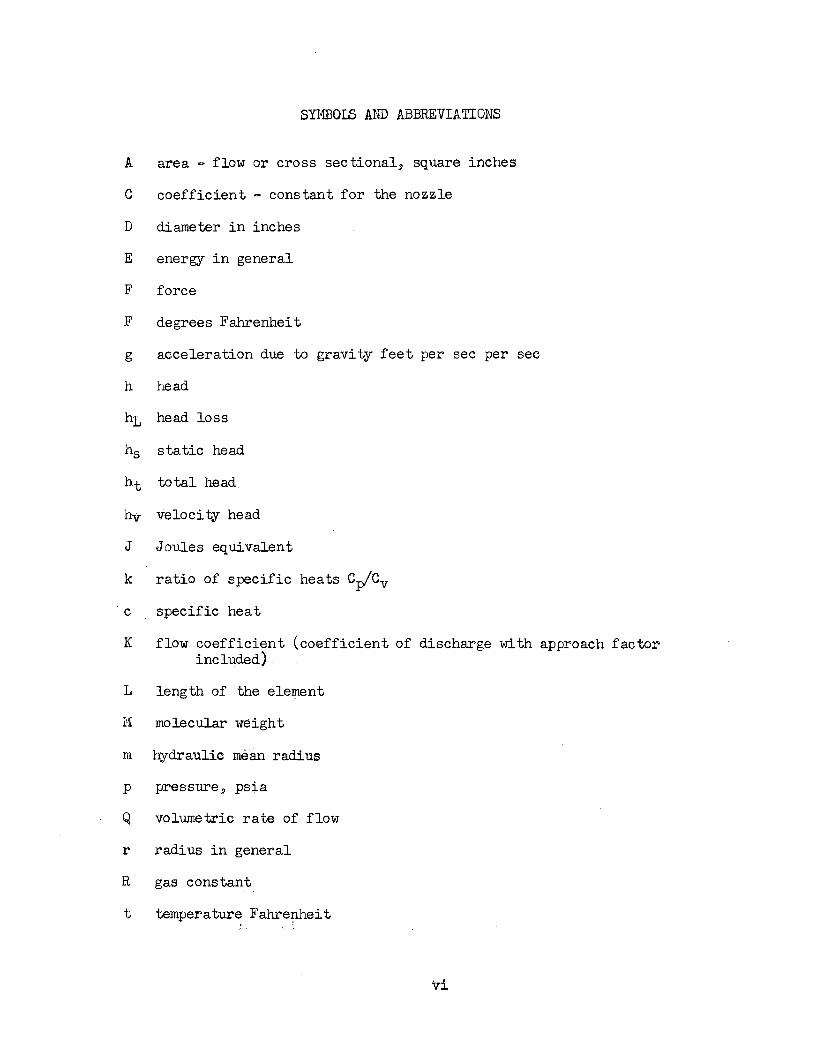
SYMBOLS AND ABBREVIATIONS

A area - flow or cross sectional, square inches

C coefficient - constant for the nozzle

D diameter in inches

E energy in general

F force

F degrees Fahrenheit

g acceleration due to gravity feet per sec per sec

h head

h1 head loss

hs static head

ht total head

hv velocity head

J Joules equivalent

k ratio of specific heats Cp/Cv

c specific heat

K flow coefficient (coefficient of discharge with approach factor included)

L length of the element

M molecular weight

m hydraulic mean radius

p pressure, psia

Q volumetric rate of flow

r radius in general

R gas constant

t temperature F' ahrenhei t

vi

V velocity feet per seconds

v volume in general

W flow rate lbs. per seconds

X unknown quantity.

Y expansion factor for the nozzle.

Z Elevation of the center of gravity of any section

Z Temperature correction factor Abbreviations

BTU British thermal units

AS.ME American Society of Mechanical Engineers

BWG Birmingham wire gage

bhp brake horse power .. : . .' • ·. .~ "I

cc cubic centimeters

ft feet.

sq square.

sec seconds ,(.'

hr hour

lb pounds:

psi pressure pounds per square inch

fps feet per second.

in.. inches

min minute

psia pounds per square inch absolute.

rpm revolution per minute.

Ra or Rd Reynold's number dimensionless

d:x./dy differential of x by differential of y

vii

Greek Letters

~ change of value in general

)-l absolute viscosity

p density

L summation of values

viii

CHAPTER I

INTRODUCTION

The measurement of the quantity of air is a vital factor in

research work dealing with carburetors and internal combustion engineso

The maximum power an internal combustion engine can develop is

dependent on the amount of air it can take in. The power and efficiency

are also affected by the air-fuel ratio.

Until recently, there were two principal methods for measuring air

consumption. The first method is the air bell method; a device employed

for many tests. Although it gives an accurate determination, it has

several drawbacks. This type of unit is very large; requires extensive

piping and is not portableo The second method uses elements of 11 kinetic

type.,t' such as orifices, venturi, and nozzles. They are simple and handy

to use, but are rather inaccurate due to the "root mean square" errors

unless the flow is quite steady. The errors can be reduced in all the

above cases by means of smoothing capacity tanks, but the size of tanks

required may be too large to be practical.

The recognition of these drawbacks lead to the design of the 11 viscous

flow air meter. tt This type of apparatus was first designed by J. F.

Alcock., The principle on which this instrurnent is based is, that the flow

across a viscous element is proportional to the pressure drop. Thus this

type of meter does not have the errors due to "root mean square." .As

there is no literature available regarding the design and experimental

results for this type of meter, the author of this paper undertook the

problem of designing and calibrating a viscous flow air meter. The

l

calibration of the viscous flow air meter is done by use of standard

nozzles described in the ASME power test codes.

2

CHAPTER II

REVIEW OF LITERATURE

There are two broad fields in the study of fluids: hyd~odynamics,

dealing with the motion of fluids, and hydrostatics, dealing with

fluids at rest. Fluids are generally divided into gases and liquids;

although the theory of fluids can be applied to both. The chief dis-

tinctions to be made are in density and compressibility. The smaller

density and greater compressibility of a gas allows it to fill the

volume of any vessel in which it is confined, whereas a small quantity

of liquid in a large vessel presents a free surface. Both types of

fluid show resistance to motion in which a further property called

viscosity is involved. In the study of the motion of fluids, the

physical properties of matter in the fluid state which have to be con-

sidered are: density, compressibility, surface tension, viscosity and

shear elasticity.

The actual motion of fluids results from the difference of pres-

sure, or of density. The fluid, whether liquid or a gas, flows in the

direction of a gradient of pressure, and from a place where the fluid

is compressed to one where it is rarefied until equilibrium is attained.

Continuous motion will occur as long as the unbalanced pressure differ-

ence is maintained by any of the external forces or difference in density~

This paper deals with hydrodynamics, or the motion of fluid; spec-

fically the flow of air has been chosen for consideration.

Before going into the details of the flow problems of air, it is

necessary to know the types of flow encountered in engineering investi-- I

gations. The most common method of determining the nature or the type

3

4

of flow of fluids is by performing simple experiments which show that

there are two entirely different types of flow in a pipe. These

simple experiments show the nature of flow in pipes, one being vis­

cous and the other turbulent, also with conditions existing between

the two. By the experiments performed with the flow of water in a

glass tube, it has been shown that if color is introduced into the

stream and the velocity of the main stream is varied, the stream of

colored water flows in a straight path at low velocities, and if the

velocity is increased, the colored filaments show a tendency to break

up at a certain 11 critical velocity. 11 At higher velocities the fila=

ments no longer flow in straight paths, but are dispersed throughout

the entire amount of fluid. The type of flow that occurs at velocities

below the "critical" is known as viscous, laminar, or streamline flowo

Such a type of flow is characterized by the shearing of concentric

cylinders of the fluid past one another in an orderly fashion. The

velocity of the fluid is greatest at the center of the pipe and de­

creases sharply to zero at the outer wall surface. At velocities

greater than the critical velocity the flow is turbulent. In turbu­

lent flow, there is random motion of the fluid particles in the direc­

tion transverse to the direction of the main flow. Even though there

is turbulence throughout a great portion of the fluid in the pipe,

there is always a thin layer known as the 11boundary11 layer or laminar

sub-layer of fluid at the pipe wall which has viscous flow. A number

of previous experiments, as well as theoretical considerations, show

that the nature of flow in pipes, whether it is viscous or turbulent 9

depends upon the pipe diameter, density, velocity of flow, and the

viscosity of the flowing fluid. The numerical value of the

dimensionless combination of these four variables is known as ReynoldHs

number. This number indicates whether the flow is viscous or turbu=

lent. Reynold's number can be stated in the form of an equation asg

Re = DVP µ,

By experiment it has been found that the flow is usually viscous for

Reynold's numbezsless than 1200 and turbulent for Reynold 1 s numbers

greater than 2200., Between these two values lies a transition region

in which the flow may be either viscous or turbulent, depending upon

the condition of flow as it enters the section being considered and

upon the roughness of the pipe walls.1

Another determining factor is friction, accompanying any fluid

flow in the pipeso There are two types of frictioni the internal

friction caused by the rubbing of the fluid particles against each

other, and the other is external friction caused by the rubbing of the

fluid particles against the pipe wall. In both cases, energy loss

due to friction is converted into heat energyo This heat energy may

be entirely absorbed by the fluid in adiabatic flow or it may be entire=

ly dissipated through the pipe walls in isothermal flow. In compress=

ible fluids some of the frictional heat may be absorbed in accelerat=

ing the fluid and yet the flow may be isothermal. In the case of the

flow of liquids and gases at atmospheric temperatures through pipes 9

we can assume the flow to be isothermal.

Adiabatic flow is generally assumed to take place in nozzles,

orifices, and short tubes through which the fluid is moving at high

1 11Flow of Fluids Through Valves., Fittings, and Pipe11 , Engr. and Research Division, Crane Company, Chicago, Ill., Tech .. paper No .. 409, May, 1942.,

6

velocities. A number of different methods of flow measurement are

available; the experimenter must choose from the available information,

the one that is best suited to the particular purpose. The selection

of a suitable method for measuring flow should be governed by the

simplicity, directness, and the degree of accuracy required. A direct

method of obtaining the flow is to collect and weigh the quantity of

fluid delivered in a given time. This method is simple and is quite

easily applied to the flow measurement of a fluid whose density is

higher than that of gaseso However$ for the flow measurement of gases

the most desirable method generally involves the measurement of some

physical effect associated with the flow. Three physical ef.fec ts that

have been found by experience to be suitable for the flow measurement

of gases are: the pressure associated with the motion; mechanical

effects, such as the rate of rotation induced in light vanes suitab]y

mounted in the stream; and the rate of cooling of a hot body, such as

an electrically heated wire introduced into the air currento Of the

three above mentioned methods, the first is of the greatest importancea

A properly designed instrument suitably inserted in the stream measures

a pressure commonly called the 11 veloci ty head11 , which is a character~

istic of the motion.. It can be measured with a suitable pressure gauge.

These instruments can be used for the measurement of air speed. The

anemometer, which is a mechanical device for measuring air speed9 depends

for its action either on mechanical or electrical effects and requires

calibration against a standard instrument .. These pressure measuring

instruments are known as pressure tube anemometers ..

Other devices which involve the measurement of pressure difference

are orifice plates, venturi tubes, and nozzles. All these measure the

pressures, not the velocity head, which depend on the dimensions and

form of the instruments themselves, as well as on the motion of the

fluid that passes through them. These have to be calibrated before

they can be used as standard~. However, the ASME has standardized

nozzles of various sizes which are used in all power test codes in

this country.

Detailed descriptions of mechanical anemometers and hot wire

• ,,

7

anemometers will not be given in this paper. However, some of the instru-

ments of the above types are convenient for practical use and have a

comparatively wide field of application.

As mentioned previously, the orifice and the venturi are the most

used devices for measuring the flow of fluids. The chief disadvantages

of the orifice plate are the element of uncertainty regarding the area of

the vena contracta and the large resistance it offers to the passage of

air through it. Both of these undesirable features have been avoided by

the use of venturi, but only at the expense of considerably increased

· cost and installation difficulties. A. well shaped nozzle, which is, in

effect, a venturi with the expansion cone removed, is a device intermediate

between the orifice and the venturi. The unrecoverable loss of pressure

through a nozzle is slightly less than that of the orifice plateD but, in

this respect, it ts inferior to the venturi. In regard to cost and ease

of installation, it is superior to the venturi.

The ttVereiu "Deutscher Ingenieure0 has standardized this form of

nozzle under the t,itl.e of ttGerman Standard Nozzle 1930. 11 The ASME has

also standardized various sizes of nozzles; and recommends their use

,1··,,,". ;:

8

for flow tests of various machines.

Any form of restriction will generate a pressure differential

which can be used as a measure of flow rate. If a non-standard pri-

mary element is to be used for flow measurement, calibration is re-

quired to establish the value of the discharge coefficient. This

discharge coefficient will not be constant in such a case over the

entire flow range due to the viscous forces, or non=uniform velocity

distribution. Charts and tables are available in the ASME test code

for use in evaluating the discharge coefficients for ASME standard

nozzles for any existing flow conditions. Hence)) the standard ASME

nozzles were selected for use in calibrating the viscous air flow meter.

This instrument can be used with pulsating flow and does not require

the assistance of a large smoothing capacity in series. It can there=

fore be used on either single or multi=cylinder engines. Alcock 1 s

viscous air flow meter proved to be very useful,in Alcock 1 s own labora=

tory. It was designed for measuring the scavenge air consumption of

high speed, two stroke research units, and the air consumed by highly

supercharged units, as well as for engines of moderate output.

There is very little information on the design.,, tests, and cali=

· bration of Alcock 1s meter available in the library, except for a brief

review of the apparatus found in Ricardo 1 s Internal Combustion Engines. The

Alcock viscous air flow meter consists essentially of a honey-comb

arrangement of narrow equilateral triangular passages 3 inches long

by .017 inches in height. The air flow through the passages is vis=

cous for flow rates within the working range of the meter.1 The

1 H. R. Richardo, High Speed Internal Combustion Engines, Vole II., London, 1923.

. /

9

resistance offered is therefore proportional to the velocity. The

"root mean square" error of the kinetic type of meter; such as the

sharp edge orifice., venturi, or nozzle is eliminated by Alcock' s meter.

The resistance is measured by a: manometer connected across the 11meter

element. 11 By special design of the manometer connections., errors due

to the flow in and out of the connections set up by pressure variation

in the line are avoided. The air passes through a cleaner and then

through the meter element. The meter element is constructed of alter­

nate layers of flat and corrugated sheet metal strips wound around a

core. The manometer connections are tubes spanning the face of the

element and having a single row of holes in each. In the upstream.

tube the holes point in a downstream. direction. In the downstream.

tube the holes point upstream. The reason for such an arrangement is

to provide a reverse kinetic head, which automatically corrects the

small kinetic pressure loss in the element due to entry effects.

The pressure drop across the elements was found to be proportional

to the gas velocity. In the case of pulsating flow in single cylinder

engines., the accuracy of measurement was unimpared. This meter was cali=

brated under steady flow conditions by comparing it with a i•German

standard nozzlfi!~ which had been checked against a "gas holder.u The. de=

sirable features of the instrument are that the pressure differential

is proportional to rate of flow and a satisfactory accuracy is obtained

over a wide range of flow.

CHAPTER III

STATEMENT OF PROBLEM

The main purpose of this investigation was to design and calibrate

an air-flow meter suitable for measuring air flow under pulsating flow

conditions. It is intended primarily for the measurement of the flow

rate of air supplied to an internal combustion engine. To attain this

objective, an air flow meter was designed on the basis of the theory

that whenever there is viscous flow of a fluid across a:rry primary element,

the rate of flow is directly proportional to the pressure drop across

the element. This is true at low values of Reynold's numbers. Based on

this theory and the previous experience of Alcock, the author designed

a viscous flow meter. The details .of construction are given in the follow=

ing pages. Standard ASME nozzles were used in the calibration of meter.

10

CHAPTER IV

ANALYSIS OF THE PROBLEM AND THEORY

\ I

The theory on which the design of the viscous flow meter. is based

involves the relationship between the flow rate and differential pressure

under special flow conditions. These conditions are governed by the

viscosity.,. which in turn depends upon the temperature of the fluid.

The Reynold's number may be used to determine the range of flow rate

over which laminar flow may be expected.

'" As the viscous flow meter was c_alibrated by use of standard nozzles,

an explanation of the equations used is presented in the appendix. The

"National Instrument Laboratories! uses the following equation to express

the relationship between the flow rate and differential pressure across

the element of a viscous flow meter.

L:l. f' = a, f> Q.2. + b /k Q

where Q is the volume flow rate

f- is the viscosity

p is the densi tu

a an.d b<·are constants

It follows from the above equation that if a flow element is designed and

constructed so that a .:: o., then the differential pressure for a partic1,1lar

fluid will be direct~ proportional to the volume flow rate.

This condition of flow will exist on:cy- for low values of the Reynold 1s

number.

The National Instrument Laboratories, Incorporation uses the Reynold's

number equation as follows.

11

12

where S equals the thickness of the flow channel.

If the flow conditions are ·such that b = o, then the pressure

differential is proportional to the square of the vol'wne flow rate. This

is the condition of flow through orifices and nozzles operating at a high

Reynold's number, and the flow is considered to be turbulent. With an

orifice operating at a high Reynold's number., flow rate errors due to

viscosity become large. Similarly, if a laminar flow meter is used for

flows above its design range, the errors due to the density of the gas

becomes an important factor. In designing the viscous flow meter the

flow channels of the viscous element are kept identical in order to

obtain the desired degree of accuracy. It has been found by the National

Instrument Laboratories, Incorporation that a high degree of accuracy is

obtained in their flow meter when the Reynold 1 s number at full scale

flow is less than 400 • '.!-

Theory of Viscous Flow

The absolute viscosity of a fluid is defined as its internal resistance

to flow. In viscous or laminar flow, the internal resrstance is due pri=

marily to the cohesive shearing stress existing between the layers tlr la.mi= -'

nae of infinitesimal t~ickness constituting the fluid stream. The shear-

ing stre~s is greater in fluids of high viscosity than in those of low ',: ..._ ..

viscosity.

For all practic~l purposes, it can be assumed that viscosity is indepen­

dent of variations iri pressure but varys wit~ temperatureo In liquids an "·')

1 N. I. Laboratories, Inc., 11Vol-O-Flo meter for Gas Measurement11

1.3

increase in temperature causes a decrease in viscosity, in gases an

increase in temperature causes an increa!3e in viscosity.'

The modern_theory of viscosity was first advanced by Sir Isaac

Newton in his monumental work ttpr~~:lL,p~au ,a.ncLdf> gener.all.Y:·,:~C>WJ'!.:;as

Newton's hypothesis of viscous flow.

In mathematical terms, Newton's Theory states that the viscosity of

a fluid is equal to the shearing stress divided by the rate of shear.

= where

,I"' is the absolute viscosity of fluid.

,·S is the unit shearing streas, F/A or, Force/Area• :,· 1 ,·j j., i.; I

A ~i:yis the rate of shear or change in velocity with respect to the

distance between shearing surfaces.

The above formula can be illustrated a.$ follows:

Fluid ),ayer station~L= 1ct-t-i--:. v­. velocity .V = 0 \

- av Plate A - St~tionary /_ ... _

\_ _,,.

,..• ______ ,.._··----.... ~-·--=-+--l------------1 t <H',.'i J::::··· =·'":'.::· ·,:::::·· 'c:::··, :::'z:=:==::t=t::==tt::======:J ,(' . ,: -~-·.:"--"' ---'--,· ..... , .. ,'---.... ·-.--... ---t---'-+,--1-1,--------1 r r

\:·{~ -~ -''· ;.. I <t tJ

_.. _____ __..,~,--4-~--4-:1-1-1-------.....-I~ 7. I--'-, •• - •• ---... ------1--1 __ _.;....__ .... _ J--._ :·--.-, -----IT I

Figl:lre 2. Newton's Theory of Viscous .Flow

.. -.,;

·1,_ ,;- \

Consider an elementary unit section of a viscous fluid filling the space

between two parallel plates A and Bin Figure 2. Assume the transverse

distance between the two plates as unity. Plate A is stationary and

plate Bis moving with a constant velocity, V. The distance between

the two plates is represented by Y.

Assume further that the fluid is in a state of steady flow with

each la~rer A Y, moving at its individual constant velocity V + D.V,

and with no layer subject to acceleration or deceleration. The fluid

layer or film closest to the surface of either plate remains fixed to

the plate by adhesion and therefore has no motion relative to the plate.

That layer of infinitesimal thickness closest'to surface A remains fixed

to plate A and does not move. Likewise, the fluid layer closest to the

surface Bis held fast to plate B by adhesion and has no motion relative

to the plate B. However, if plate Bis moving with a constant velocity

Vs relat:i,.ve· to plate A, then the fluid layer adhering to plate B also

moves with constant velocity V relatively to the fluid layer adhering to

plate A. It is therefore evident that no shearing action takes place

between the fluid and the plate to which it adheres~ but takes place only

between the fluid layers.

It is assumed that the fluid layers are of the same size and shape,

and the shearing stress between any two layers or the adhesion between

the fluid and the plates is equal and opposite to the force,9 F, produc=

ing flow.

i,e. S = F

Sis the total shearing stress

Fis the force producing flow

Ifs is the unit shearing stress between any two fluid layers, then

s equals F/A.

A is equal to the shearing area of fluid layer.

Then., •

From Figure 2, it is evident that the sum of · A. Y is equal to Y

and the· sum of the elementary velocity. AV is equal to V •

therefore, ~ = F/A ffl

or ,, - F/L 2 = FT Force x Time - = (L/T)/ L T2 Length~

If CGS units are used in the above formul~ the unit of absolute

viscosity will be the poise. Thus the poise is the force in dynes per,.

sq·cm at·a velocity of one cm per sec at a distance of one cm.

Viscous Flow in Capillary Tubes

UThe work of the French physician and scientist, Poisseuille,

in whose honor the unit of absolute viscosity, the npoise11 , was

n~ec;i,,d~~much to confirm and illuminate Newton's hypothesis of . " •. '; . ,:.· '· : l .· .. .:· ~ '•

v:i,.scoµ~ flow.i~ capillaries or smal],. tubes. Poisseuille's ex-.. '••: ,.' · ,ii. ' i I ,.,,•!,I '

periments made in about the year 1840 we~e undertaken in an . ' . . _;

effort.to.~etermine the nature of the .:f'low of blood in the

h~~n ya~<?ular 1system. This experimenta~ work w1,s not done :_. J ' • • ..

intl:lnfi.q;naliy. for the purpose of cpt).firming a theory of fluid .. : ····. ". ',,. , .. ,.: .. , : ,; ......

meehiili:j'.e~,''but that is exactly whaJ,. it did. Unfortunately, it ·:, •,.. •:,"

wa~ :hbt'iµriJl>after his death, when''Ei, mathematical analysis was '·

mad.e o:f' his·· findings, that the real value of P9is!Se::Uille 's work

15

as a major cbntribution to fluid mecp.anics was discovered. Poisse­

uiii~'t{:La~ :iri the light of mathematical' ~alysis forms the b~sis

of th~ modern theory of viscous flow in tubes·, capillari~s and pipes."2

2 Mc9lairi., Clifford. "Fluid Flow in Pil)$stt, New York Industrial Press, 1952~

16

It is interesting to study in detail Poisseu.ille I s Law. A small

capillary tube of radius ( r) and length (1) is shown in the figure on the

next page, through which a viscous flui.d is flowing. It is assumed that

the fluid is in a state of steady flow, that is to say the layer is

moving at constant velocity, and no layer is subjected to acceleration

or deceleration. Under such conditions the fluid is in equilibrium with

respect to external forces. It is assumed that the layer of the fluid

adhering to the surface of the tube has zero velocity and the maximum

velocity is at the center of the tube. The pressure (P) existing at

the entrance or upstream end of the tube is entirely dissipated in

overcoming the flow resistance throughout the entire length (L) result­

ing in zero pressure at the exit' or downstream end of the tube. Since

the pressure drops at a constant rate per unit of length throughout the

tube, the unit pressure drop is equal to P/L.

The flow in a tube can be assumed to consist of an infinite number

of hollow concentric telescopic cylinders of unit length and with w~ll

thickness dy.

The constant velocity of individual conoentriq cylinders is progressiyely

greater toward the center of the tube by a small increment dv. The flow

rate past any transverse section of the stream must be constant. Other­

wise, the flow would be distorted and result in turbulence.

If one cylinder is farther downstream than another, the pressure

exerted on its upstream end is less than that exerted on the other cy­

linder in proportion to the distance by which it leads the other cylinder

at a given time. There would be a similar difference in the pressure

exerted on the downstream end of the cylinder. The ends of the fluid

17

Shearing Stress ~~ilj Velocity profile, a parabola, formed

by elementary fluid cylinders.

Pexit = 0

dV Section - aa

L

Capillary wall Figure 3., Viscous Flow in Capillary Tube

c~rlinders have the shape of an annular ring with it' will thickness of ( dy).

Therefor~, by equating the equal and opposite forces and using the

theorem of Pappus for finding the area of the ends of the hollow cylinders

for any cylinder of unit length

p 2 ;r y L dy = 2 -,rs (y + dy)

for the entire length 1 of the tube

2 7T y P dy = 2 ;r s ( y + dy) L

for the entire stream

J 2 7T y P dy 12 rr s (y + dy)L 2 . . .

7T" Y P = 2rr y s L

therefore shearing stress s = rr y2. P = 27ry L

E 21

From the equation obtained for the shearing stress it can be seen that

the shearing stress varies with the distance (y) from the axis of the

tubeo

\

18

In the case of simple viscous flow, the shearing stress is the same

for each fluid layer and is independent of the distance (y).

Newton's expression for unit shearing stress in a differential

form is

s = - f" d-V ay

The reason for the negative sign is that y is measured from the center of

the tube and not from the outer edge of the tube.

Therefore

rate of shear =

_ a dV = z!:. I dy 21

dV _ ay -

p -L 2Lf"

From ~his expression it can be shown that the rate of shear is not constant

for each fluid cylinder, but varies with y when P, L, ~ndfk remain constant.

In simple viscous flow the rate of shear is the same for each fluid layer.

The· velocity changes as a uniform or straight line function and the shear~

ing areas are the same for each lay-er.

It is desirable now to find an expression for the velocity of any

fluid cylinder at any distance y frqm the axis of the tube, and then a

general equation for viscous flow in a tube can be established

dV = - yP dy ¥ 2

V=- YP -,.c ~

therefore

where C is a constant of integration. '-·.

Since the velocity is zero at the tube walls when y equals the radius

of the t 'l\\}~ • '1

= r2 P C 4L,,.U,

p V = 4Lf4"

Hence, it is established that the velocity gradient of the telescopic

fluid cylinders takes a form of a solid parabola within the tube shown

in Figure 3. The volume of fluid flowing through the tube during an

interval of time can now be obtained. The above expression gives the

velocity of the fluid cylinder located at a distance (y) from the axis

19

of the tube in terms of distance per second. Since the distance travelled

in unit time is the same as the velocity~ the total volume flowing int

sec, will be the sum of all these elemental volumes multiplied by to

Thus

• •

volume= area x velocity x time

V :

V :

- 7TPt 21f

: lTPt r4 BLf-

''

- "TTPt r4 - 81 V

The driving force in terms of fluid head is h: P/w

where his the head in feet of flowing fluid

w is the specific weight of the fluid equal pg

pis the density of the flowing fluid

g is the acceleration of the gravity

Therefore, = 7ffJghr4t 81 V

eo

The volumetric flow rate of an incompressible fluid can be expressed

as Q = V

t or V: Q t

Q is the volumetric flow rate cubic units/sec

vis the volume of fluid flowing int sec

tis the duration of flow in sec

therefore,

fl' = rr f:. g h r4

8 L Q

or 7TP g h r4 Q = 8 L j1-

According to the law of continuity, the quantity of fluid flowing per

second through any pipe is expressed as Q = VA.

V is the mean velocity of fluid or uni ts of length per sec. For

a round pipe, the above formula becomes

Therefore,

V iT r2 =

or h: 8LVJ.{.

P gr2

where h = (h1 - h2) = ht

h1 = head lost in producing flow against viscous resistance.

In deriving the fundamental equation stated above, it is assumed

that the entire pressure head is converted into velocity head. Thus

Usually the above equation is written in terms of the pressure

differential for the section of pipe being considered.

21

It can be written: AP=f>gh

where A p is the pressure drop across a transverse section of the pipe

under consideration causing the flow of the fluid. Thus

Q =

This equation for the flow is developed for circular cross section pi~.

The same equation can be applied to any other section., if only a factor

lmown as hydraulic mean radius is taken into account. Therefore, the

above equation can be expressed in terms of hydraulic mean radius· (m)

to be applied to different shape sections,

m =

l!"or a circular pipe

m:

cross sectional area wetted perimeter

£ = r 27Tr 2

where r is the radius of the pipe, or r = 2m.

Therefore,

or

.. .

Q:7TApl6m4 BL,"

Q = 2rrm4 . AP Lf-

For fluid flowing through a given section

Hence, let 21rm4 L = a'

Where a I is a constant, then

2 rrm4 is constant • L

This proves that when the flow is entirely viscous or streamlined:, then

flow is directly proportional to the pressure drop. This cam. be written

as A p = a"f'- Q

where a11 is a constant.

CHAPTER V

THE DESIGN OF THE VISCOUS FLOW ELEMENT

The viscous flow element chosen for this design consists of a

honeycomb of long narrow triangular passages 5.,2 11 long, each having a

cross sectional area of,0.0019 square inches.

The honeycomb element was formed by use of two long strips of

aluminum, .005 in. thick and 5~2 in. wide, one plain and the other

corrugated. One strip was placed on top of the other and the pair of

sn:i~ts we:fe' then wound around acentral core. It thus formed a cylind­

rical element having triangular passages with a length of 5.2 in.

parallel to the axis of the cylinder ..

The corrugated aluminum strip is stocfmaterial, used in a certain

model of oil filter manufactured by the Fram Corporation.. The avail=

ability of this material from the Fran1 Corporation was the reason it·

was selected for use in this design ..

The size of the triangular sections of the passages formed by the

aluminum sheets is shown below. The dimensions were obtained by taking

a number of impressioIBof the triangular passageways on paper and

averaging the measurements.

A

Figure 4o Section of the Triangular Passage

22

In Figure 4 AB ;: 1/16 in. AD= 0.0413 in.

perimeter ·= 3/32 + 2/16 = 7/32 in.

area= 0.0413 x 1/2 x 3/32 = .0019 sq,in.

hydraulic radius=

=

cross sectional area wetted perimeter

.OOl9 = 0 0087 i'n 7/32 • •

23

Reynolds number may be used as an indicator of the probable velocity

at which a change in the type of flow may be expected.

In engineering installations using actual pipe, it is usually

found that the critical point corresponds to a Reynolds number of 1200.

The following calculations based on a Reynolds number of 1200 will be

used to establish the upper 1imi t of the flow range in which laminar

flow may be expected. Reynolds number may be calculated using the

following equation.

Re = DVp P-

where Dis the diameter, equals 4 x hydraulic mean radius

µ is the viseosi cy-, lbs sec per -sq ft

V is the velocity, ft per sec

fJ is the density, slugs per cubic foot.

The viscosity of air at 80°F and 14.7 psia is

;,<,= p =

= D =

Re = V =

3.87 x 10-7 lbs sec per sq ft

1 - l.4.7 X 144 ~ ~ 53.3 X 540 X 32.2

2.28 x 10-3 slugs per cubic foot

4 X 000087: 0.0029 ft 12

DVP or V : ReP., µ "1rp

1200 X- 3.87 X l0-7 0.0029 X 2.2S X 10-3

= 70.0 ft per sec.

24

...., = 70.0 ft per sec.

It was tentatively assumed that the air 'meter capacity should be

at least 7 cfs. This value is the estimated air flow requirement for

a truck engine to be tested using the meter.

The area required for a Reynolds number of 1200, and velocity of

70.0 ft per sec is calculated as

A= ~ = to x 144 = 14.4 sq in

The percentage of area taken up by the metal is 27.2%, hence

The total area is

1.27 x 14.4 = 18.2 sq in

and the diameter required for the viscous element, having a central

core of 0.5 in. diameter, is calculated

TID2 ,rd2 __ 4 - 4 total area ·

where Dis the diameter of the viscous element

dis the diameter of the core

K (n2 - c12) = 1a.3

D2 _ ct2: 18.3 X 4

Thus D = 4.83 in.

In the case of air flow between parallel plates, it was ·'found l?Y

Orr that turbulent conditions could exist at Reynolq's numbers as low

as 117.1 Therefore, for the air meter capacity of 7 cfs it is desirable

to base the viscous element diameter cm. a lower value of Reynold's number

to insure laminar flow. Also the pressure drop across the viscous

and Heat Transmission.

element, is accurately measured at low Reynold's number.

Different values for diameters are determined corresponding to

Reynold's numbers lower than 1200, and are tabulated in Table 1.

TABLE l

'._.~_'.) _! Re ··Na. Velocity Flow area Total area DiameteI Differential fps sq in. sq in. in Pressure.

psf · in.of H20 .. ·\..,:,t:'

5.85 16.7 100 173 220 3.77 0.725

l~d· 7.04 144 207 16.2 4.55 o.875 ..

140 8.20 123 1>6 14.05 5.30 1.02 { ''~ :.

160 \.~~]5 108 137 13.2 6.os 1.16 ,d

180 ;LP•? 96.2 122 12.4 6.80 1.31 ,, .. ·· ·;,, / ..

200 11.7 86.2 ~ :, .:· ·.- ~ ,. 10~ .. 2 11.7

," <J 7.56 1.45

400 23.4 43.2 55.q 8.38 15.20 2 .. 92 ',/1 ~ ·, ,· . 1-.

600 35.2 28.7 34.2 6.60 22.8 4.38

800 46.8 21.6 27.2 5.a8 30.3 \ 5.82

1000 58.5 17.3 22.0 .5.30 37.8 7.26

1200 70.0 14.4 18.3 4.83 45.2 8.70

The pressure drop across the viscous element is obtained by the formula

AP: 2~VL m

where 6P is the pressure drop, lbs per sq ft

fl' is the viscosity, lbs sec per sq ft

Vis the velocity, ft per sec

Lis the length of the viscous element, ft

mis the hydraulic mean radius, ft

For air at 80°F and l.4.7 lbs per sq in.

/"' = 3.87 x 10-7 lbs sec per sq ft

V = 70 ft per sec at Re= 1200

and for the viscous element

L = 5.2 in. or 0.43.3 ft

m. = 0.00072 ft ;"~ .. :· .

Thus substituting in the above. fomula .

2 X 3.87 X 10-7 X 0043.3 X 70 A, p = 2 ,_... ( .00072)

= 45.2 psf

= 8.70 in. of watero

In order to use the meter for measuring larger air flow rates on engines

other than the tested engines, it is desired to design the viscous

element to have a larger diameter.and corresponding smaller Reynold's

number. However, the pressure drop should be large enough for satis­

factory accuracy. Wi.th this subject in mind, and to make use o~ the •, .

material available, a diameter of 14 in. is selected for the viscous

element.

l . .z~ "it-A f

./

A

3 1/ 21-1.<;-

N F L B E D --- C m

------ -

G H J ~ 1~4" .., 21" ~ 3 1 / 2

I I==--=--=--=--=-- __ 10" 6 3 " ~ I

Figure 5. Viscous Air Flow Meter

~o Of Figure 6. Static Pressure Tube

,,

I\)

-.J

. I \

. ' \ \ \ \

\\ '\.'- -' ' -­' "-' ..... ......

I \

J ) J

:·.I I I I - / I; I - / .- ./ / J ; / ;/ --

,,.,,/' . . --------~---_______ ___.,....,.,.,,..----··

Figure 7. Sectional View of the Viscous Element

28

CHAPTER VI

DESCRIPTION OF THE APPARATUS AND EQUIPMENT

The housing of the viscous air-flow meter is made of galvanized

iron. It is composed of three sections: the central cylin~icuu

section (B) flanged at both ends, and the two end conical sections CA) f:,; I

and (C) having a flange at one end, tapering to a four inch diameter

cylindrical section at the other end. The end section (C). is provided

with short cylindrj.c~l. section at the flanged end to house the filter-

ing element.

The end sections (A) and (C) are fixed to the central section (B)

by means of bolts. The central section (B) ,~loses the viscous

element (G) and static pressure tubes (E).

A schematic view of the viscous air-flow meter is shown in

Figure 5.

Filtering Element (D)

The filtering element (D) consists of a cylind,ricaJ.;. element

made pf hardware cloth packed with copper turnings. It is soaked in

a sui}~ble filte'r oil, and the excess oil is drained off before it

is asseJllbled in position in the meter.

Viscous Element CG)

The viscous element (G) consists of a honeycomb of triangular

pass~ges, made-by winding a pair of aluminum strips, one corrugated

and the other plain, over a central wooden core. The diameter of the

viscous element is 14 in. and the length is 5.2 in. This is assem-

bled in section (B) in the space provided, and is fixed in position

by means of a wooden strip (K) of 1/2 in. square section, set screw

(I) and the small metall~c angles (L) soldered to the housing .. The

29

space between the element and the inside of the housing is packed

with cotton to avoid the leaks. The assembly is shown in Figure 5.·

Static Pressure Tubes (E)

The arrangement of the static pressure tubes is shown in Figure

5. These two metallic tubes are l/2tt inside diameter and 25 in. long,

and fixed in the housing at right angles to each other. On these tubes

small radial holes of 1/32 in. in diameter are drilled in two rows

making an angle of 60° with respe~tive to each other, as shown in

Figure 6. These holes are 1/2 in. apart center to center. By this

arrangement a true static pos~tive pressure can be measured. In

order to make air-tight connections between the tubes and the housing

four sockets and packing nuts (F) carrying 10 1 ring seals are provided.

Figure 6 shows the arrangement and the direction of the static

pressure tubes.

The whole assembly of the meter is fixed on a telescopic stand.

by means of which the meter can be adjusted to any desired height.

This whole arrangement can be seen in Figure 12 and 13.

A temporary collar and adapter arrangement is provided to install

the different standard size nozzles which are used in the calibration

of the meter. This arrangement is shown in Figur-e 13. A.t the inlet

side of the meter a sleeve Cm) is provided for inserting the thermometer

in the air stream. Pressure tap joints and connections are made air

tight with sealing compound. The pressure drop across the element /-- ..

was measured by means of a draft gage and standard water manometer.

The manometer connections were made by means of rubber tubing. This

arrangement is shown in Figures 10 and l3e The pressure taps at the

nozzle throats are made according to the specification given in

ASME Power Test Code. A complete arrangement of the meter is

shown in Figures ]2 and 13.

Before the mcc.er was calibrated, a check was made to see that

31

all the connections and flange joints were air tight and the draft gage

was level.

Also the mid point between the two rows of holes on both static

pressure tubes should face upstream. This is to insure an accurate

measurement of the pressure drop across the viscous flow element.

32

Figure 8, VIEW OF THE FILTER AND VISCOUS EIEMENT

Figure 9, CIOSE UP VIEW OF THE VISCOUS EIEMENT SHOHING TRIANGULAR HONEYCOMB

33

Figure 10, VIEW OF THE MANOMETERS

Figure 11, VIEW OF THE ENGINE TESTED

Figure 12., ASSEl\ffiIED VIEW OF THE VISCOUS AIR F' row METER

34

Figure 13, VIEW OF THE ARRANGEMENT OF APPARATUS AND TESTING EQUIPMENI'

CHAPTER VII

PROCEDURE

The equipment for calibration was set up and connected to the

engine as shown in Figure 13. The outlet of the air-flow meter was

connected to the air cleaner inlet of the engine. The draft gage and

manometer were leveled and the draft gage scale was adjusted to zero.

The 13/8 in. nozzle was installed in the nozzle holder at the inlet

end of the air meter and the manometer connections were made. After

the preliminary check up of the engine to be used, the test was

begun.

The engine was operated at various loads and speeds to obtain

the desired rates of air flow through the nozzle and air meter.

Simultaneous readings of the manometers were taken to obtain the

pressure drop for the nozzle and the air meter .at each of the selected

test conditions. The operating conditions were controlled so as to

vary the pressure drop for the nozzle within the range specified by

the ASME Power Test Code. The same procedure was repeated for each

of the following nozzle nozes: 1 in., 3/4 in. and 1/2 in.

The barometric pressure and the temperature of the air were

observed several times during each group of tests and the average

value of each was recorded for the test.

35

Obsercved Data

GHAPrER VIII

DA.TA

The data observed during the test are recorded in Tables 2 and

3 for different nozzles. These tabies show the pressure drop across

the nozzle PN· (in. of oil specific gravity .85) and corresponding

pressure drop PM across J;,he meter ( in. of water) • The manometer

readings ~ere corrected to inches of water and recorded in the Tables

of Calculated Data.

Calculated Data

The calculated data are recorded in Tables 4 and .5 for the

different nozzles. The expansion factor (Y) used in calculating

the flow through the nozzles is also included.

The results obtained from the observed and calculated data are

shown in the following graphs:

Figure 14:

Figure 1.5:

~igure 16:

Figure 17:

Figure 18: " . ~

Pressure drop across the nozzle versus pressure drop across the meter (from observed data).

Rate of flow versus the pressure drop across the meter (from the calibration data using lin, 3/4 in. and 1 3/8 in nozzle).

Rate of flow versus the pressure drop across the meter (from

1the calibration data using 1/2 in. nozzle).

Rate of i'low versus the pressure drop across the meter at standard conditions (6o°F and 14.7 psia) •.

Graph tor the temperature correction.

Sample calculation is shown in the Appendix B.

,.: ·:1;.

36

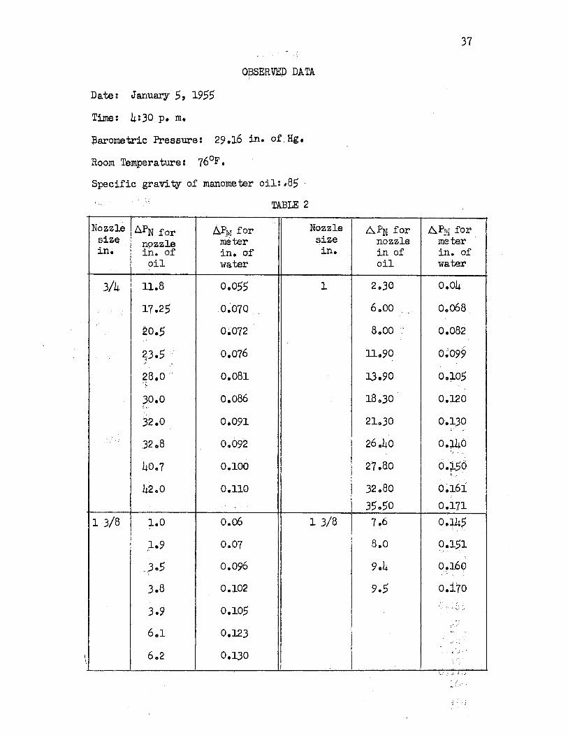
O~SERVED DATA

Date: January 5, 1955

Time: 4:30 P• m.

l3arometric Pressure: 29 .J.6 in. 0£. Hg•

Room Temperature: 76°F •

Specific gravity 0£ manometer oil: 185 :

Nozzle L°lPN for size nozzle in. in. of

3/4

... · .i' ~ '

l J/8

oil

11.8

17.25

~0.5 ,~i '

~3.5 . ~8.o ,. l·

.30.0 b

j~.o

32.B

40.7

42.0

1.0

,;i.9

}•5

J.8

6.1

I 6.2

A.PM for meter in. of water

0.055

. 0~070.

0;072

0.081

0.086

0.091

0.092

0.100

0.110

o.o6

0.07

0.096

0.102

0.105

0.123

0.130

TABLE 2

Nozzle size in.

l

1 J/8

6.111 for nozzle in of oil

2.30

6.oo ...

a.oo ....

11.90

13.90

18.30

21.30

26.40

27.80

32.80

35.50 7.6

s.o 9.4

9.5

37

APM for meter in. of water

0.04

o.068

0.082

0~099

O.:L05

0.120

0-.130 \.,!.· •·

~ ..

d.;t50 .... ,.··

0~161 0.171

0.145 '. ~-'

~.15:t

q"i60 -,, .. ~ . ·'" -.-

o.170

..

., - ., .. _:·

38 OBSERVED DA TA

Date: January 6, 1955

Time: 4:30 p. m.

Barometric Pressure: 29.455 in. of hg.

Room Temperature: 77°F

Density of the Manometer Fluid: .85 for nozzle

TABLE 3

Manometer Reading Manorooter Reading in. of H20 in. of H20

Nozzle LPN .6. 111 Nozzle NN A,P size in. for nozzle for meter size in. for riozzle for m~ter

1/2 4.35 0.012 1/2 15.50 0.026

6.80 0.016 17.00 0.027

9.10 0.018 20.50 0.029 I,

10.7 . , , 0.020 · 22.50 0.031

11.0 0.021 23.50 0.032

13.2 0.023 26.60 0.035

14.25 0.024 27.80 0.0351

15.00 0.025 28.60 0.0352

CALCUIA TED DA TA

Barometric pressure: . 29.1611 of Hg.

Room temperature: 76°F

Density of air: .0720 lbs/cu. ft at 70°F.

Discharge coefficient: .984 for the nozzle.

TABLE 4

fize of Corrected 6.PN lb Expansion 6I}i in. ozzle 6..PN ~n. of per sq factor Y of H20

~o in.

3/4 ~0.01 .36 .980 .055

14.66 .526 .977 .070

17.41 .626 .974 .072

20.00 .720 ·212 . ' .076

23.80 .855 .~69 .081

25.50 .916 .9,62 .086

27.40 .982 .959 .091

27.90 1.005 .958 .092

34.60 1.245 .948 .100

35.70 1.285 .947 .110

1 1.95 .070 1.000 .04

5.10 .184 .994 .o68

6.8 .244 .9,82 .082

10.1 .364 .979 .099

11.8 .425 .982 .105

15.5 .560 .979 .120

18.l .651 .973 .130

22.4 .8o6 .968 .140

39

..6.PM lb w lb per sq per sec.

in.

.00198 .o46

.00252 .056

.00259 .o61

.00274 .o65

.00292 .070

.00310 .072

.00328 .075

.00331 .078

.00360 .085

.00396 .087

• • 00144 .037

.00259 .057

.00295 .o68 "

.00256 .083

.00396 .090

.00432 .102

.00468 .110

.00505 .120

Size of Corrected ~PN lb nozzle A P1f in per sq

in. of H2o in.

l 23.6

27.8 J ··.,'

39.2.

.850

1.000

Expansion AI}{ in ~ lb factor Y of ~O per sq

.996

.959

.954·

in •

.15 • Q0540

.J.61 .00580

.171 .oo615

l 3/8 "i .-ss i.615

.031 1.03 .06 .00216

.002,2

.00346

.00367

.00.378

2.97

3.23

3.32

5.26

,.19

6.45

6.80

8.oo

8.o6

.058 1.03

.107

.116

.119

.189

.187

.232

.244

.288

.290

1.00

1.gi, ,. . . # _.I ,,.

l~Ql_,.

•2Q~ ::•./ ,),.t,

-~~~ .990

~989

.984

.983

.102

.105 .,

.130 .00468

.123 .• 00442

.145 .00522

.151 .00543

.160 .00575

.i70 .00012

40

w lb. per sec.

.124

.134

.145

.047

.o65

.086

.091

.092

.114

.1o6

.126

.129

.1~8

.J.40

CALCULA T&D DA TA

Barometric Pressure: 29.455 in. of Hq = 14045 lbs per sq in.

Room Temperature: 77°F

Density of Air: .0726 lbs per cu ft.

Discharge Coefficient: .970

Density of the Manometer Fluid: .85 for no.zzle

TABLE 5 •I

Size of 6PN Corrected Expansion 6.PM nozzle lb per ~PN Factor in~of H20

in. sq in. in. of ··H20 y

1/2 .133 3.70 .991 .012

.208 5.78 1.000 .016

.278 7.74 .9~7 .018 /': .,;,

.328 9.10 .986 .020 Ii , , :' ·,. J ~ ,''

.336 9.35 .9,85 .021 <!;)

.4Q3 11.20 .9,84 .023 '··''

.435 12.10 .982 .024

.437 12.75 .980 .025 . I i" f

.475 13.20 .9,79a .026 ,: .!

·?2Q 14.42 0978 .027

.626 17.40 .9,74 .029

.688 19.10 .972 .031

.716 19.90 .971 .032

.810 22.60 .969 .035

.850 23.60 .965 .0351

~875 24.30 .964 .0352

APM lb per sq in.

.000432

.000575

.000648

.000720

.000756

.000828

.000865

.000900

.000935

.000972

.00104

.00111

.OOll~

.00126

.001262

.001270

41

w lb per sec.

.0107

.0135

.0155

.0167

.0172

.0186

.0192

.0193

.0200

.0210

.0230

.0240

.0244

.0260

.0264

.0268

,.

, 1

1 Pninb, orl1/::111 o:~,~ / ....

-_/

-,, _, <~ Pair ts ~or lJ 21 ro·,zll.E • ,

""' /

2

/ -., _., /

,. _,,,

V _.,,v _,.,v .

/

.,......v

_,v

Figure 14. Pressure Drop Across Air Flow Meter Versus Pressure Drop Across Nozzles.

42

_,

/

60 100

43

Q • 21 :=+~~""t-r-+.-+:.++-+··+-__ Hc---H--+_-:::_"t.t-:+,'=t-~~~-~""'=-+-+:"+-++::++-++--+-H-i-Ht--::--11-++-++::+-i-++-+H-t-Ht--::-i-~""'=-++-++-++-++--tr+-t---+-+--+··~+.:::::=:=~=:~=::t-.:=-~~HH--H t-+-t--·+-t-t·- - ·- -- · - --t-+-t-t-t-H---1 +-1-iH--t-+-t-+-t-+- HHH-t-+-+-t-+-t-b-1--t-t-+-+-++-t· · 1- - i-- ·++-+-t-t-t-t·-+-+-+-t-t·

·- · ··· ··· · - -· --- · -+-H-+-t-+-+-+-t-+-+-HH-+-+-+-+++-HH-t-+-+-t-+-+++-+-t--t-t·-+-+--1-1---t-++-+++-+--t-+-t--

o.20HH-+-t-+-+++-+-+--H-+++++-+--HHH-+-+++-+-+-HH-+-++++-+-1---H-+-+-+-+-+-+-HH-+-+-+-+-+-+-HHH-+-+-+++-+-+--H-+--t

o.19HHH-+-+-+++-+-+--H-+-+-+++-+--HHH-+-+++-+-+-HH-+-+-+-+-+-+--1---H-+-+-+-+-+-+-HH-+-+-+-+-+-+-+--HH-+-+-+++-+-+--H-+--t t-t-t-+-+-+-+-·>-+--+-+-···-l~H-+-+-+++-+-t-tH-+-++++-+-+--HH-+-+-+-+-+-+-HH-++-+-+-+-+-HH-t--t-+-+-++-+-+--H-+-+-+++-+--H t-t-t~-+++-+-+-i-~++--H-.H_-+-+-+-+-++-+-+--1-+-+-+-+++-+--HHH-+-+-+-++-+-HH-+-+-+-+-+-+-HH-++-+-+-+-t-+--H-+-+-+-+-H

I ,..- Y! 1o;.:; m I~

O.lpt-+-t-+-+-+-+-++-t-H-+-+-+-+-++-+-HHH-++++-+-+--HH-++++-++-t-+--t-++++-++-HH-+-+-+-+-++-HH-+-+-++++-+-HH--H

Q~15HH-++++-t-t-t-+-t-++-t-t-t-++-+-+-+-t-t-+-+-+-+-+-t-t-+-+-+-+-+-t-tH-++-+-+-+-HH-+++-+-HH-++++-HH-+-+-++-HH~

HH-1--+-t--t+-+-+-+---+-+-+-++-+-t-HHH-+-+-t-+-+-+-HH-+-+-+-++-+--HH-++ ----t-+-t-+-+++-+-t-t-++-+-+-+-t-tH-+--l-t-ti/r/H=L

b.14 EE±fftttttt±mBE±EEHE±EEmmffttffttBHllE±EE!EEmM HH-++-+-+-++-+-·H-++- --t--t-+-+-+-+-+--H-++-+-+-t-+-+-HH--+-+-+++-t--i-HH-+-++-+-+-+-HH-+-+ t-+--H--++-+--YH© f~=== ,. ----0.1~ HH-++-+-+-++-+-+--H-+-+-+++-+-+--HH-++-+-++-+-HH-+-++-+-+-+--1---H-+-+-+-+-+-+-+--H--+-+-+-+-++-+-+--H-·:JJ.. HH-+-+++-H

--+-+-+-+-1-+-+-+-+-+-+-+-+-1-+---+-+-+-+--+-+-+--+-+--+-+-+-+--+-·+-+-+---+ -t-+-+-H-+-+++-+-HH-++-t-t-HHi,7f'1.,'-t,lr.i;l;I', t--+-+-+-+-+--+-+--+---t

1--1-+--+--+-+ +-+-+-+-+--+-+---c--+--~-+-+-i--+ +-+-+-1-+-+-+-+-+-+-+-+-1-+---+-+-+--c--+--+-+--+-+-i--+-+-+--+--+-+-+-+-i-+ l(.'~;-+->---i--+-+-+-+-+-+-+-1-+---+

0 o 12 ~-c ++-++-HH-1-1--+-+--1--t-1 c--c-- -,-+-+-+-+·H +-t-1---HH-+-+-++++-HH-+-+-iH-+'-t--t-+-HH-+-t--+-+-+-+-HH-+-+-+-+-i-t-H~

HH-+-+++++-HHH-+-+-++-+-+-HHH-+-+++-+-+-HH-+-+-+-++-+-HH-+-+-+-+-i-t-+-t-llrn,~'lv:'t--+--HH-+-t-++-HH-+-+-++-t-H

O.llH--1-++++++-+--H-++++++-+--Hl-+-+++++++--f+-l++++++--H--1++++++-+-+;,~~0·}~HH-+-+-+-+-+-+-HH-+-+-+-+--1--t-1 I/

HHH-+-+-+-++--HHH-+-+-+-t-+-t-+--HH-+-+-+-++-+-HH-+-+-+-+-i-t-HH-+-+-+-·~~+-+--i-t-HH-t-+-+-+-t-t-HHH-+-+-++-H o.10HH-+-+-+-+-++-HH-+-+-++++-+-HHH-++++-+-+--H-+-++++--+-t-1-t-1-++-b'f-'=t-t-+-HH-+-++-+-+--+-t-HH-+-+-+-+-++-+--H

.08

.07

.06

.05

• 04

.03

HH-+-+-+-+-++-+-+---+-+-+-++-+-+-HHH-+-+-+-++-+-HH-+-++--+-+·-~ .. ~tttt:m::tt:tttt:m::tt:UttU::::tt=ttl -• E/:~HH-+-+-+-++-+-HH-+-+-+-++-+-HHH-+-t-++-t-+-HH-+--f

HH-+-+-+-+-t-+-t-t-l-+-+-+-++-+-+-+--HH-+-+-+-++-+-l-++,0•1+,.:J;../H---H---l-+++-H--1--l-+++++-+--H-++++++H~f--H-++-I

HH-+-+++-t-t-t-+-t-++-t-t-t-+-+-+-+-+-t-t-+G:$F+--,r+-t-t-+-+-t-+-+-HH-+-+-+-++-+-HH-+-+-+-+++-+-HH-+-+-++-+-+-+-HH-+-, • r,,

I/

H-+++++l-+-l-+++++--H--Ht(t»+++--f+-l--++++++-H--1-++++++-+-H-++++++-+--Hl-+-+++++++-f+-l+++++-l

•• -

/

_.03 .04 ,,05 .06 •• 07 .08 .,99 .10 .:1.;t .12 -.,;1;;3 .14 •. i.5 .16 ,.17

Figure 15.

Pressure drop across meter, in. of water.

Calibration Graph for Meter using 3/4 in., l in., and 1 3/8 ~n. nozzles at 76°F and 14.30 psia.

.030

.029

.028

.027

.026

0025

0024

. .023 0 Q) (/)

H 0022 8. ~ .021 .. ~ .020 q $-i

•rl .019 ('J

~ 0 .018 Q)

~ .017

.016

.015

.014

.013

.012

.011

•

--

- -1-1-1-1- - 1-· r - -1-1--- -· -

~-- •·<*

-~ ~ --} I

" '/

IF

-----J

·-)

)

~1- - I/ . ,_ ··r·

·-- - I/

I

-I/ -

IJ

I/

I )

)

)

./

-) -/

1 l'!>.~

I I

01 .015 .02 .025 .03 .03::> .04

Pressure drop across meterJ in. of water

Figure 16. Meter Calibration Graph using J/2 in. nozzle at 77°F. and 14.45 psia.

44

,_ . ,_

.~

-1-1-1-

.04 5

• Q (I) fl)

H a ~

C')

! r+-1

I'.-! •rl ro

0 • 1~ 11111111 i I ! ! 111111 i 1111111111111111111111 t 111111111111111 i 1111 1111111111 00 111111111 i 11111111111111 1111!1117111 1111111!11 !Ill!

17

,r I

I

y._:d3 l l i[ i lTTTT

!

mffilllllli i

0 •081 I I I I I I I 1111111111111 i 1111111 i 11111111 i 11 lffil I I I I I I i I I 111111111111 i I I I I I I I I I Ii I I I I I I I I I I I I I I I I I I I I i I r:.;

r:;; 1 t

flli

ed o. 06111111111111111 i 1111 I I I 11111111 IH1Il l LLD 1111 l I I I 1111 U Li 1111111 U Li I Uli 11 W LUii i J LLILUIETil11 I ~ (1j ~

1 ...

i/ I/

V V

o • 041 I I I I I ! I I 111 I 11 I I I I I J:f I I l 11 : I I I I I I I I I I I I I I I I I I I I I I I I I I I I I i I I I I I I I I I I I : I I I I I 11 I I 11 I I I I 111 I I I 11 I 11 tttti I i

! l

r;; vrrn

D

0 • 021 Uf tllfljffl 1111111111111111111111111111111111111111111111111111111111111111111111111 i 111111111 IJJ§

FT IJ1 I I I I I I I I I 111111111111111 i 1111111 · 1 ·11· 111 ! I I I I I I I f I l I / 111111111 ! 111111111111111111 : 111111 i I i ; 111 i+ 0. 01 [J'.1~ 111 I 11 111 I I 11 I I I 111 I 11 11 I I 11 i I 111 I I 1111 I I I 11 I I 111 I I 11 I I I I +- I I I I I I I I ! I I ! I I I i I I I I ! I I I I I I I I I I I I ! I ! I ! !

.01. .02 .04 .06 .os .10 .12 ,11~- .16 Pressu:ce drop across meter, in. of water

F:i.gU:t\':') 1?. JYleter Calibration Graph at Sta-1d.ar·d Conditions [6o°F. and 14.7 psial

.18 • 20

,I::'"' Vl

46. I

- - ·- -- ~ · 1-- e- -·+-+-· >-4--+4-·++· 1-4--1-+-'-+·4-++-+-++....-+-+-i-+-<-+-1-t-<-+-++-++-4-++-+-+-+-+-+-t-t· -+-+-++++-+-· .- -- - - -· "'- ·· -· - ..._ - - ·--- -· • 1--,i-- -- -1--1-- -1-

-i..-1-- - '-· · - 1-- --1--1-- -+-+-+-+-++-+-~-t--+-t-t-+t-+-r+-H-t-+·+-+++++-t-+-H-t-t-++- - t--t- ·+-<-+-+-+-+-+-+-++-4-++- '-~-'-~ ·· 1-. - -1-- - --t-l-Hl-+-f-t-t-t-+-+·++++++-H-H-H-+-,r+-1-+t-++-+·l--t-t· t--r- --+-t-+-+-+-+-·t-<-t-+-4·-+-+

· ~-1-1--1- -++++-+-+-+-t-H-+-l-t-1-+-t-++-+·1-++t-+-t--+-t-+-t-H-t-·t-- ·t-- ·· - ·+-+-+-+-·H-+--t-+-t-

1-++-++-+-++"'k-+..11c'-:·,·-H-t++++++++t-H-H--H-t--H-H-++++++++-t-t-H-H--HH-H-H-++rt--i--t-t·+++-+-+-+-H

0990 ,,

' I' '"

'"

I'\

~r~- --~~-l-l-+++++-+-+~--+-~-t+++++++++++--H:>.t--i-+-H-t+-H-++++-1-1-+++++-+-HH-H-H-t++-t--t-H

I' I'

I' I"\

'" I"\

0970

'

60 65 70 75 80 85 90 95 Tempera tu.re °F

Figure 18. Temperature Correction Graph

CHAPTER IX

SUMMARY A:ND CONCLUSIONS

According to the theory on which the design of the viscous air

flow meter was based, the pressure drop that occurs during laminar

flow is directly proportional to the rate of flow of air.

The results of the tests as presented in Figure 15, ip,· anq 17

show a linear relationship between the pressure drop across the meter

and the flow. This indicates that laminar flow was obtained for all

rates of flow used during the tests. The meter was calibrated, by

measuring the rate of flow through ASME standard nozzles of different

sizes. Figure 14 shows that the pressure drop across the nozzle versus ~. !

the pressure drop across the meter plotted on log paper is a straight

line with a slope of approximately J/2. This also indicates that

laminar flow through the meter was obtained since the theoretical re=

lationship indicates that the graph should be a straight line w.i. th a

., slope of J/2. From the observed and calculated data9 a calibration

graph, Figure 17, for the meter at standard conditions was obtained.

The flow rate (W) at temperatures other than standard tempera­

ture may be obtained by use of the correction factor (Z)' from Figure

18. The flow rate (W} must be mul~~plied by an additional correction .barometer reading psi

factor . · 14. 7 to correct for the effect of atmos-

pheric pressure. The size of the viscous element was made large enough

to hand:;J.e the total capacity of air flow to an engine considerably

larger than the one used for the tests.

(,., 47

Conclusion

From the data obtained and calibration graphs, it was established

that the flow of air through the meter was laminar. From the data

obtained for the pressure drops on the nozzles it is seen that for the

]/2n nozzle the pressure drop measurements were not obtained very

accuratezy. This is due to the fact that as the air flow increased

the manometer readings fluctuated _considerabzy. This indicates the

presence of pressure: pulsations which would affect the accuracy of

flow measurement.

From the various graphs and calculated data it was established

that the capacity of viscous element was underes tim.a ted. However, the

small pressure drop resulting from the large capacity may be an ad-

vantage. For internal combustion engines testing it is desirable

that the pressure drop across the meter be no larger than is necessary

for satisfactory accuracy in the measurement of the pressure drop.

From the graphs it is seen that almost all of the experimental

points are either on or close to the line through the average or" the

points. This indicates that satisfactory accuracy was obtained in

taking the readings. The rates of flow obtained on the tests are

considerabzy larger than the claculated value obtained from the

theoretical equation on which the design was based. This equation

contains a constant based on experimental results. It seems possible

that the constant might have a different numerical value for the size

and shape of flow passages used in this design. It also seems possible

that the high velocity and turbulence associated with the air issuing

from the noz~les affected the rate of flowo

46

Recommendations for Future Research

Additional tests and investigation might be undertaken to

establish the maximum flow capacity of the meter within the laminar

flow range.

This would require a larger engine or other machine to produce

a larger flow rate. It would also be desirable to determine why the

flow obtained from theory used in the design does not agree with the

value obtained from the experimental results.

49

BIBLIOGRAPHY

Oliver Ernest, Measurement of Air Flow, Chapman and Hall Ltd, London 1933.

Louis Gess and R. Do ~rwin, Flow Meter Engj,neering Handbook., The.Brown Instrument Co., 1946. ·

H. F. Purday, An Introduction to the Mechanics of Viscous Flow. Dover Publication, Inc., 19490

L. K. Spink, Principles and Practices of Flow Meter Engj,neering, The Finkboard Co., 1947.

B. o. Buckland., ttFluid Meter Nozzlestt 9 Transactions ASME,9 Vol. 56 P• 827, 1934. - .

Ho K! Lind.en, ttAir Flow Through Small Orifices in Viscous Region,u Transactions of· ASME, PP• 48-A-93, 1948.

ttFlow Measurements", Part 5.o, ASME Power Test Codes 9 1949.

"Displacement Compressors VacuUill PUillps and Blowers 11 , ASME Power Test Codes, 1939.

"Pressure Measurements," Part 2. ASME Power Test Codes 2 1942. -- '

Linford, "Flow Measurement and Meters,'' ASME Transactions, 19420 .• '

H. R. Ricardo, High Speed Internal Combustion Engines, Vol. Il, London 1923.

uvo1 .. 0-Flow Meter for Accurate Gas Flow Measurement. 11 National Instrument Laboratories, Inc.

•. Clifford H. McClain, HFluid' Flow in Pipes ...

D. s. Ellis, Elements of draulic En ineerin , 3rd edition, D. Van Nostrand Co., inc. New York, London, 19 7.

Ho Addison, l:\Ydraulic Measurements., John Wiley and Sons, Ltd., New York 19410

Hubert 0 0 Croft, Thermodynamics, Fluid Flow and Heat Transmission, McGraw-Hill Book Co., New York, 19.38.

APPENDIX A

FLOW OF FLUID THROUGH A NOZZLE

The equation presented in this section is for the flow of fluids

through a well shaped ASME standard nozzle in which it is assumed

that the outlet pressure will always be more than 53% of. .~lle in1et

pressure. (1) (2)

up~tream downstream

Fig

A section view of an ASME standard nozzle is shown in the above

figure.

In deriving the formula for flow through such a nozzle, tl:1.e

following assumptions are made. The flow of air through the nozzl~

is assumed to be steady, and isentropic. The fluid flowing conforms

to the law pv = wRT and Cv remains constant. If these conditions hold

true, the energy per lb of fluid will b~ the same at both sections 1

and 2, ·and the actual rate of flow is g:i.ven

_W = V2 A2 P 2 (referring to section 2) ..

where Wis the actual rate of flow, lb per sec

V2 is the velocity of air ft per sec

p 2 is the density of air lb per cu ft.

Hence W = A2

51

52

:and W ( actual) = CW (theoret.ical)

where C ~ij the coefficient of discharge.. The value of C is obtained

from experimental results. This is sometimes combined with the

velocity of approach factor

K - C - -../ I - (D2/D1)b

where K = flow coefficient.

The nozzle inlet is exposed to the atmosphere and hence K is equal to

C as D1 is infinite.

The ref ore W :;: A2C to/ 2 g Ii AP

where /Ji is the density of the fluid at sectio~ (1). This equation is

used for liquids only, and for compress~ble fluids like a gas or air,

isentropic flow being considered, a factor known as the expansion

factor (Y) and also the factor (E) known as area multiplier for the

thermal expansion of the nozzle to be taken into consideration.

Hence a general formula for the rate of flow for a compressable

fluid flowing through a nozzle is given as

l

k is the ratio of specific heats

P1 and P2 are the pressure

of air at sections (1) and (2) respectively.

In the above equation D1 is infinite in the present applicationj hence

the second factor of the equation is unity, and

l 11Flow Measurementstt., ASME Power Test Code, 1949.

;:J • ·,, ;,J

The velocity- of approach factor k .. and "Gherrnal expansion factor · ..... c,,:. '•Lf' ·.·,:·. . t .. :', ... ;'. :·,, ..

E and ~e negligable; thus (k) becomes equal to the coefficient of l,.>. 7. ·'\;_ ff:~ -

discharge (C) and the equation for the rate of flow is ,,--,

W = .668 A2 C YJ f1AP

This equation was used in the calculation of the flow rate through

the nozzle

APPENDIX B

SAMPLE CALCULATIONS

Barometric pressure= 29.455 in. of Hg

: 29.455 X 0491: 14.45 psi

Room temperature= 77°F or 537°F abs.

Density of air at 77°F = 0.726 lb per cu ft.

Discharge coefficient= .970 for 1/2 in nozzle (ASME Code).

Pressure drop across the l/2 in nozzle

b.I'N = 13.20 in of H20

= 13.20 x .036 = .475 lb per sq in.

The gravimetric rate of flow of air through the nozzle is given as

W • .688 ACY / /'16.P lb per sec

where A= area of the nozzle throat, sq in.

G = coefficient of discharge for the nozzle

Y = expansion factor

[k 2/k : [k-1 (P2/P1)

1 ( I )(k-1)/k]' 1/2. - P2 P1

1 - P2!P1 . ,\

k = 1.39 Ratio of specific heat of air

P2 = pressure downstream, lb per sq in.

P1 = pressure ~pstream, lb per sq in.

AP= p1- p2, lb per sq in.

= density of the air, lb per cu ft. Nozzle throat area (A)

A - rrn2 - 1I 1 o 196 · ... ~ - 4 X 4 : • · sq in.

where Dis the nozzle throat diameter.

54

, ..

Expansion factor

y =ck . Pl-AP 2/k . k-1 ( Pl ) .

k-1 1-( PP1- AP) ,-

1-(PJ __ - ~p) P1

55

1/2

substituting the values, in this equation

y : [1.39 (14.45 - .475) 211•39

1.39-1 14.!iS - .475 1.39

.39 ,- 14045 14.45 l -

1 -

: [56 ( • 967) 1·44. ( l-0 .967) • 2sl 112

1-- (1-0.967) _J . ~ 0.0091[1/2 -[ ;i1/2

:: L.56 x .952 x 0•033.J - o.95~

: 0.978

W;: Q.668 X .196 X 0.970 X 0.978 / 000726 X 00475

- 0.0230 lb per sec.

1/2

At this rate of flow the pressure drop across the viscous element was

0.026 in of water. Calculation for the temperature, pressure and I

vi~cosity correction is as follows: .

6 p :: 2 ~ LV m

at standard conditions of 6o°F and 14.7 psia

21 .6.. P6o = jii2' /"60 V6o and at arw other temperature t°F

/ 6.Pt = ~ jl't Vt

assuming 6,. p60 = ~ Pt

µ 60 v6o =Jlt Vt or V6o = ~ Vt

Therefore W6o = ~6o x P6o :: A V 60 f 60 and

Wt = Qt Pt = A Vt ft

d o - P Pi6o P6o an r - RT or --n-t = . ·. / r+. r·Pt

60 Tt

Thus f6o _

Tt

X P6Q X Tt Pt 160

56

or W6o :: Wt 14.7 Tt X -x

Pt 520

For a temperature of 77° F and pressure of 14.45 lb per sq in.

Wt = W77 = 0.023 lb per see

/it -::!f'*n =.0185 centipoise andµ,60 = .0180 centipoise

W60: 0.023 X .0185 X 14o7 X 537 .018 I'Ii:45 520

: 0.023 X lo08

= .0248 lb per sec.

W - j.l., 6b Pt ·. t -~ X 14.7 X

_520 X w6· .. Tt 0

= Z W6o

Where Z is the correction factor.

z =/,L60 x Pt X 520 .JZ"';: 14. 7 T t

Hence correction factor Z is obtained for a temperature of 77°F and

14.7 lb per sq in.

z - wt - 1 :: 0.926 - ~o - 1.08

Hence Wt= W6o x 00926.

If the pressure drop~ Pm across the meter is lalown, the corres=

ponding W6o may be obtained from the grapp. The correction factor

at the desired temperature is obtained from the correction factor

graph Figure l 8 and hence the true rate of flow at 6.. Pm may be

obtained corrected for pressure temperature and viscosity as shown

above• Additional correction factor (Barometer reading psia divided

by 14.7) to be multiplied by rate of flow for pressure correction. ' /

VITA

s. Vicar Husain candidate for the degree of

MASTER OF SCIENCE

Thesis: DESIGN AND CALIBRATION OF A VISCOUS AIR FLOW METER

Major: Mechanical Engineering (power)

Biographical and Other Items:

·Bern June 15, 1928 at Hyderabad Dn. India

Undergraduate Study: Bachelor o,f Science, Nizams College Hyderabad, 1947. Bachelor of Science in Mechanical Engineering, Osmania University, Hyderabad Dn. India, 1949.

Graduate Study: Oklahom~ A & M College, 1953-1955.

. Eit,ei-ience: Two years of'" indu~trial training, spoft'~8retf''bf . . . the Government of India., at Hindustan Aircraft Factory,

o: . India and Cooper En~neering Ltd. {Diesel Engine Manu­"£acture), Satara, in.du.; Cone year at each). One yeaz:- part time . teaching at Oklahoma A & M C'ollege

.. for the Physics :Department. · 1

··"' IU - ,

Date of Final Examination: May; 1955 ,I_'

57

THESIS TITLE: DESIGN AND CALIBRATION OF A VISCOUS AIR FLOW METER

AUTHOR: S. Vicar Husain

THESIS ADVISER: Professor W. H~ Easton

The content and form·have been checked and approved by the author and thesis adviser. The Graduate School Office assumes no responsibility for errors either in form or content. The copies are sent to the bindery just as they are approved by the author and faculty adviser.

TYPIST: Sara Preston