1914ch6

P1: shibu/Vijay

August 12, 2005 10:42 1914 1914˙C006

6Determining an Optimal Fleet Mixand Schedules: Part I — Single Sourceand Destination

Hanif D. Sherali and Salem M. Al-Yakoob

CONTENTS

6.1 Introduction: Problem Description . . . . . . . . . . . . . . . . . . 1376.2 Related Literature . . . . . . . . . . . . . . . . . . . . . . . . . . . . 1396.3 Modeling Preliminaries . . . . . . . . . . . . . . . . . . . . . . . . 143

6.3.1 Problem Notation and Assumptions . . . . . . . . . . . . . 1436.3.2 Penalty Functions . . . . . . . . . . . . . . . . . . . . . . . . 144

6.4 Model Development . . . . . . . . . . . . . . . . . . . . . . . . . . 1456.4.1 Model Variables . . . . . . . . . . . . . . . . . . . . . . . . . 1466.4.2 Model Constraints . . . . . . . . . . . . . . . . . . . . . . . 1476.4.3 Objective Function . . . . . . . . . . . . . . . . . . . . . . . 1486.4.4 Overall Model Formulation . . . . . . . . . . . . . . . . . . 149

6.5 An Aggregate Formulation AVSP for Model VSP . . . . . . . . . . 1506.5.1 Formulation of Model AVSP . . . . . . . . . . . . . . . . . . 150

6.5.1.1 Objective Function and Constraints . . . . . . . . 1526.5.1.2 Extracting Schedules for Individual Vessels . . . . 152

6.6 Computational Results and Rolling Horizon Heuristics . . . . . . 1536.6.1 Computational Experience in Solving

Models VSP and AVSP . . . . . . . . . . . . . . . . . . . . . 1536.6.2 Rolling Horizon Algorithms . . . . . . . . . . . . . . . . . . 1546.6.3 Comparison with an ad-hoc Scheduling Procedure . . . . . 157

6.7 Summary, Conclusions, and Future Research . . . . . . . . . . . . 159References . . . . . . . . . . . . . . . . . . . . . . . . . . . . . . . . . . . 160

6.1 Introduction: Problem Description

Efficient scheduling of oceanic transportation vessels presents serious chal-lenges to concerned decision-makers due to the complexity of the operationand the potential savings that can be attained. A vessel usually costs tens of

137© 2006 by Taylor & Francis Group, LLC

P1: shibu/Vijay

August 12, 2005 10:42 1914 1914˙C006

138 Integer Programming: Theory and Practice

millions of U.S. dollars with daily operational costs amounting to tens of thou-sands of U.S. dollars. Chartering and spot-chartering of vessels is also veryexpensive and should be avoided to the extent possible. In general, large-scale vessel scheduling is very intricate and requires repeated revampingto accommodate changes in demand, market conditions, and weather effects.Manual approaches are often inefficient and expensive, and hence, it is imper-ative to utilize quantitative methods to generate and update vessel schedulesefficiently and in a timely fashion.

The problem that is studied in this chapter is concerned with the trans-portation of a product from a single source to a single destination. The nextchapter examines the case of multiple sources and destinations, along withthe option of leasing transshipment depots. For example, we might be in-terested in shipping crude oil from a refinery to a storage facility that has aknown demand structure defined by different daily consumption rates. Thedaily export from the source depends on the availability of the product at thesource, the availability of vessels, and the current storage level at the desti-nation’s storage facility. Consumption rates at the destination might not befixed during the entire time horizon and might vary based on, for example,seasonal considerations. The level of the product at the destination’s storagefacility is desired to lie within certain lower and upper bounds, and hence,daily penalties are imposed based on limited shortage or excess quantitieswith respect to these bounds.

Typically the organization that handles the transportation of the productfrom the source to the destination owns vessels of different types, where eachtype is characterized by the vessel size, speed, loading and unloading times,etc. Moreover, there are vessels that are available for chartering during all orpart of the time horizon. Spot-chartering is also available if desired, wherebya vessel is chartered for a particular voyage or voyages, not for a period oftime. In this case, all operating costs are undertaken by the vessel owner. (See

The organization aims to satisfy demand requirements at a minimum over-all cost that is comprised of operational expenses, penalties resulting fromexceeding lower and upper storage levels, and chartering expenses. This re-quires an efficient utilization of the organization’s self-owned vessels, and aminimal reliance on chartered and spot-chartered vessels that tend to havehigh associated costs. The combinatorial nature of this problem makes themanual scheduling of vessels inefficient and costly because of unduly highresulting chartering and penalty expenses.

In this chapter, we develop mathematical models that generatecost-effectivevessel schedules in a timely fashion. The problem described above is faced bymany oil companies such as the Kuwait Petroleum Corporation (KPC), whichis required by agreed upon contracts to meet specified demands of crude oilthat vary based on daily consumption rates at a given destination. The sin-gle source-destination vessel scheduling operation arises in many situations,for example, when large quantities of crude oil need to be transported fromKuwait to a destination located in Europe, North America, or Asia. In this case,

© 2006 by Taylor & Francis Group, LLC

for example, Rana and Vickson [24].)

P1: shibu/Vijay

August 12, 2005 10:42 1914 1914˙C006

Determining an Optimal Fleet Mix and Schedules 139

the destination might be a single customer or a collection of customers thatare located within close proximities of each other. Hence, the single sourceand destination problem considered herein, although a special case of themultiple source and destination problem addressed elsewhere [31], is impor-tant in its own right and is frequently faced in practice.

6.2 Related Literature

Transportation routing and scheduling problems have been widely researchedin the literature, with a bulk of the published work dealing with vehiclerouting and scheduling problems. Vessel scheduling, in particular, has at-tracted the least attention among all transportation modes. Ronen [26, 27]highlighted a noticeable scarcity of published research dealing with design-ing, planning, and managing sea-borne transportation systems, and gave anumber of impediments associated with vessel-scheduling problems such asthe complexity and the high uncertainties associated with such problems.However, recently, there has been increasing interest in research related tomaritime transportation as evidenced, for example, by a special issue de-voted to this area in Transportation Science (Psaraftis [23]). Also, the book byPerakis [20] gives an overview of models for a number of problems related tofleet operations and deployment. For a comprehensive review on ship rout-ing and scheduling research conducted over the last decade, the reader may

In order to accurately model vessel routing and scheduling problems, novelmathematical formulations are often needed. Moreover, models for large-scale vessel scheduling problems are rather hard to solve due to complexconstraint structures that result from the operational intricacies of such prob-lems, and their inherent combinatorial characteristics arising from an explicitconsideration of the different components of the operation. Vessel schedulingcan therefore be an arduous and time-consuming task, and is often compli-cated by the dynamic nature of such problems. Yet, many organizations stilllargely handle their vessel scheduling problems only manually.

Typically there are three modes of operation in seaborne shipping: liner,

to bus or passenger train lines. Tramp ships operate like a taxi by following

fleet of ships. Accordingly, vessel routing and scheduling problems can bepartitioned into four categories: a) liner, b) tramp, c) industrial, and d) otherrelated models. The first three are not sharply defined or mutually exclusive,nor collectively exhaustive (Lawrence [17]); hence, the fourth category ofproblems captures applications that cannot be clearly classified as liner, tramp,or industrial. It is worth mentioning that water transportation routing andscheduling models mainly deal with the transport and delivery of cargo.


the available cargos. In industrial shipping, the cargo owner controls the

[17]). Liners operate based on a fixed published itinerary and schedule similar

refer to Christiansen et al. [8].

tramp, and industrial (see, for example, Christiansen et al. [8] and Lawrence

P1: shibu/Vijay

August 12, 2005 10:42 1914 1914˙C006


Considerably fewer models have been developed to tackle vessel routingand scheduling problems in the context of transporting passengers. This isa result of the fact that most vessels move cargo around the world, whilepassengers mainly travel by air or land.

The literature on modeling techniques and approaches for the liner ship-ping is fairly limited; however, in recent years an increased activity in this area

erating costs for a fleet of liner ships involved in various routes. It was shown,based on real liner shipping data, that substantial savings could be achievedvia using the proposed modeling approach. Note that the work of Powell andPerakis [22] was an extension to the work of Perakis and Jaramillo [19] andJaramillo and Perakis [13]. In the latter two papers, a linear programmingapproach was used to solve a fleet deployment problem. Cho and Perakis [6]investigated a fleet size and design of a liner routing problem for a containershipping company. The problem was formulated by generating a subset ofcandidate routes for the different ships a priori, and was then solved as a lin-ear program, where the columns represent the candidate routes. This modelwas also extended to a mixed-integer program that additionally incorporatesinvestment alternatives for expanding fleet capacity. Xinlian et al. [31] formu-lated a fleet planning model for a problem similar to that investigated by Choand Perakis [6]. The model aims to determine the ship types to add to theexisting fleet of ships as well as an optimal fleet deployment plan.

Datz et al. [9] developed a simple calculative method for scheduling a linerand suggested some techniques for evaluating the financial results of such aschedule. Nemhauser and Yu [18] studied a model for rail service that can beused for a liner problem. Dynamic programming was used to find the optimalfrequency of services that maximizes profit over the planning horizon. De-mand for service was a function of two variables, namely service frequencyand timing. Rana and Vickson [24] developed a deterministic mathematicalprogramming model for optimally routing a chartered container vessel. Theformulation involves nonlinearities, which were handled by converting thenonlinear problem into a number of mixed-integer programs. Benders’ de-composition was applied to the resulting mixed-integer programs, whereinthe integer network subprograms were solved by a specialized algorithm.Later, Rana and Vickson [25] extended their work in [24] by allowing multipleships. They formulated a mathematical programming model for a container-ship routing problem that determines the following: 1) an optimal sequenceof ports of call for each vessel, 2) the number of trips each vessel makes in theplanning horizon, and 3) the amount of cargo delivered between any two portsby each ship. The problem was solved by Lagrangian relaxation by decom-posing it into several sub-problems, one for each vessel. Each sub-problemwas further decomposed into a number of mixed-integer programs. For otherrelated literature on liner models, the reader may refer to Christiansen et al.


has become evident (see, for example, Christiansen et al. [8] and Lane et al.[16]). Powell and Perakis [22] formulated an integer programming model for afleet deployment problem. The objective of the model was to minimize the op-

[8] and Al-Yakoob [1].

P1: shibu/Vijay

August 12, 2005 10:42 1914 1914˙C006


Very little research has been conducted on the allocation, routing, and

a ship scheduling problem obtained from a Swedish ship-owning company.In this problem, a ship-owning company was engaged in world-wide oper-

for the planning period, which covered 2 to 4 months. The author designedan algorithm that used the Dantzig-Wolf decomposition method for linearprogramming, where the subprograms were modeled as network flow prob-lems and were solved by dynamic programming. The master program in thedecomposition algorithm was modeled as a linear program having only zero-one elements in the matrix and on the right-hand-side. This algorithm wastested on instances involving about 40 ships and 50 cargos.

Later, Appelgren [3] utilized integer programming methods to solve a ves-sel scheduling problem. The problem was to determine an optimal sequenceof cargos for each vessel in a given fleet during a specified time period. Thispaper was an attempt to deal with some of the shortcomings associated withthe technique used by the author in [2], where a decomposition algorithmwas used, which, however, produced nonintegral solutions that could not beinterpreted as valid schedules. To avoid fractional solutions, a branch-and-bound algorithm was developed, where the branching was performed on oneof the ”essential” noninteger variables and the bounds were computed bythe decomposition algorithm. A decision support system for both tramp andindustrial shipping was described in Fagerholt [10], where a heuristic hybridsearch algorithm was employed for solving such ship scheduling problems.

Since the problem under consideration can be classified as an industrialshipping problem, we present next some industrial scheduling literature thatis most closely related to our problem.

A vessel scheduling problem concerned with transporting crude oil fromthe Middle East to Europe and North America was considered by Brownet al. [5], who formulated a mixed-integer partitioning model and utilizedcolumn generation techniques to solve this problem. The demand structurewas specified by a sequence of cargos that needed to be delivered during theplanning horizon. The approach adopted by Brown et al. [5] attempted togenerate a partial set of complete feasible schedules (in a column generationframework), along with the generated schedules’ costs, and then utilized anelastic set partitioning programming model to derive a prescribed solution.This same problem was investigated by Perakis and Bremer [21] who alsoapplied a set partitioning approach to solve the problem. The work of Brownet al. [5] was extended in Bausch et al. [4] by allowing a shipload to have upto five products. A similar set partitioning approach to that of Brown et al. [5]was used by Bausch et al. [4] to solve the problem.

Sherali et al. [30] presented mixed-integer programming models and spe-cialized rolling horizon algorithms for an oil tanker routing and schedulingproblem to ship various products from one source to different destinations.The demand structure that was investigated by Sherali et al. [30] was deter-mined by the total demand for each product at each destination, along with


scheduling of tramp shipping (see Appelgren [2, 3]). Appelgren [2] discussed

ations involving a large number of vessels. A set of cargos were provided

P1: shibu/Vijay

August 12, 2005 10:42 1914 1914˙C006


the respective sub-demand that was required to be satisfied within agreed-upon time intervals. It was assumed that some vessels could carry more thanone product. The modeling approach adopted in Sherali et al. [30] as well asin this chapter differs from the modeling approach of Brown et al. [5] in that itcombines the process of constructing and selecting feasible schedules at once.

Ronen [28] proposed a mixed-integer programming model and a cost-basedheuristic procedure for a vessel transportation problem that is similar to theone considered in this chapter. The approach adopted by Ronen [28] separatesthe solution of the problem into two stages. The first stage determines the slateof shipments to be made, and the second stage generates vessel schedules. Incontrast, the models developed here decide upon the fleet size mix as well asthe detailed vessel schedules all together. Another application within the oilindustry, which involves the transport of refined oil products from a refineryto several depots, was investigated by Scott [29]. A Lagrangian relaxationapproach was adopted to generate a set of potentially good schedules, andan enhanced version of Benders’ decomposition was used to decide upon anoptimal schedule from within the generated set of schedules. Fagerholt andChristiansen [11] studied a multi-product scheduling problem similar to theone presented by Bausch et al. [4]. However, in this paper, the authors as-sumed that each ship in the fleet is equipped with a flexible cargo hold thatcan be partitioned into many holds in a specified number of ways. A setpartitioning approach was utilized by the authors for this problem and a de-tailed algorithm for finding optimal schedules for the individual ships wasdescribed in Fagerholt and Christiansen [12]. An inventory-routing problemwas studied by Christiansen [7], which attempts to attain a degree of balancein the ammonia supply at all producing and/or consuming company-ownedplants around the world.

A ship scheduling problem that does not clearly fall into liner, tramp, or in-dustrial shipping was investigated by Koenigsberg and Lam [14] who studiedqueuing aspects for a small system of liquid gas tankers operating in closedroutes between a small number of terminals. For any particular system, theirmodel provides the expected number of ships at each stage, the expectednumber waiting in each stage, and most importantly, the expected waitingtime at ports. Exponential service time distributions were used; however, aseries of parallel simulation computations were also employed to analyze theimpact of other distributions. Later, Koenigsberg and Meyers [15] extendedthe work of Koenigsberg and Lam [14] by developing an analytical model ofa system having two independent fleets that share a common loading port.Exponential distributions of service times were used in all queuing stages. Theauthors used a simulation program to investigate the behavior of the systemwhen the service time distributions were not exponential and demonstrated agood level of conformity between the simulation and the analytical results forexponential distributions.

For further details on vessel routing and scheduling problems and models,


the reader may refer to Al-Yakoob [1], Christiansen [8], Perakis [20], andRonen [26, 27].

P1: shibu/Vijay

August 12, 2005 10:42 1914 1914˙C006


Although many vessel scheduling problems and models have been discuss-ed in the aforementioned literature, none of these fully address the peculiaraspects of the problem considered in this chapter. The specific nature of thedemand structure and the consideration of different vessel types and costcomponents require novel mathematical formulations and solution methodsto accurately model the problem and to derive solutions in a manner thatcan be practically implemented. The remainder of this chapter is organizedas follows. The next section provides a detailed description of the problem. Amixed-integer programming model is then developed in Section 6.4, and sub-sequently, an aggregate reformulation of this model is derived in Section 6.5.Solution algorithms and computational results are presented in Section 6.6,along with a comparison with the ad-hoc scheduling procedure that is cur-rently in use at KPC. Finally, Section 6.7 provides a summary and some con-cluding remarks.

6.3 Modeling Preliminaries

This section introduces aspects of the problem that will be used to formulateinteger programming models in Section 6.4 and Section 6.5. In particular,Section 6.3.1 presents notation and assumptions, and Section 6.3.2 describesa function for computing penalties associated with exceeding certain lowerand upper allowable storage levels. For the reader’s convenience, a glossary

6.3.1 Problem Notation and Assumptions

Let h = 1, . . . , H index the days of the time horizon under consideration.Typically, a time horizon is associated with a contract to deliver the productfrom the source to the destination based on some given consumption ratesas discussed in Section 6.1. Therefore, the terms “time horizon” and “con-tract horizon” will henceforth be used interchangeably. Note that a contractmay be signed, and then another contract may be signed prior to the end ofthe first contract horizon. Suppose that there are T vessel types, indexed byt = 1, . . . , T . It is assumed that vessels of the same type have similar featuressuch as capacity, speed, loading and unloading times, etc. The capacity of avessel of type t is denoted by t and the total number of vessels of this typethat are available for use during all or part of the time-horizon is given by Mt

(note that Mt is composed of self-owned vessels in addition to vessels that areavailable for chartering). For a vessel type t ∈ 1, . . . , T, let n = 1, . . . , Mt

index all vessels of this type, and let Ot and C Ht = Mt − Ot respectivelydenote the number of self-owned vessels and the number of available vesselsof this type that can be possibly chartered. Accordingly, let n = 1, . . . , Ot andn = Ot + 1, . . . , Ot + CHt ≡ Mt respectively index self-owned vessels andvessels that are available for chartering of type t. Let us also denote O =T

t=1 Ot and CH = Tt=1CHt. Let $t,n be the cost (in U.S. dollars) of chartering


of notation (sequenced in order of appearance) is provided in Appendix A.

P1: shibu/Vijay

August 12, 2005 10:42 1914 1914˙C006


a vessel n of type t, for n = Ot + 1, . . . , Ot + CHt = Mt, and for each t ∈1, . . . , T. Let UTt,n be the maximum number of days vessel n of type t canbe used during the time horizon. This time restriction is typically needed formaintenance purposes.

Let Tt represent the time required to load a vessel of type t at the source,plus the time this vessel takes to travel from the source to the destination,unload time at the destination, and then travel back from the destinationto the source. We assume that there is a unique prescribed route from thesource to the destination, and likewise, from the destination to the source. LetTt = T1,t + T2,t, where T1,t is the time required to load a vessel of type t at thesource plus and then travel to the destination, and T2,t is the time required tounload at the destination and then travel back to the source. Vessels of the sametype are assumed to have equal values of Tt (and their splits), and this durationis also assumed to be independent of h; i.e., Tt is independent of the day the legstarts (weather effects are neglected). The values of Tt and its splits are derivedfrom the design speed of the vessels of type t. Let DCt,n denote the dailyoperational cost of vessel n of type t so that the total operational cost of vesseln of type t is given by Ct,n = Tt(DCt,n), which covers the round-trip expensesfrom the source to the destination, and is independent of the day the trip starts.

Let Q denote a production capacity or certain imposed quota of the productat the source. At the beginning of the time horizon, the storage level at thedestination is given by w. This level may represent a single storage facilityor a collection of storage facilities at the destination; however, for the sakeof modeling, we only deal with a combined aggregate storage level. Let SL1and SL2 denote the minimum and maximum desired levels, respectively, atthe destination’s storage facility, which should be maintained to the extentpossible in order to avoid penalties. Accordingly, letπ denote the daily penaltyfor each shortage or excess unit at the destination. The permitted shortageand excess quantities at the destination with respect to the desired levelsSL1 and SL2 to the extent given by A1 and A2, respectively. Let b1 = SL1 −A1 and b2 = SL2 + A2. Let U B > b2 be a sufficiently large upper bound on themaximum allowable storage level on any given day of the time horizon. Short-ages levels falling below b1 or in excess of b2 (up to UB), while permitted, arehighly undesirable, and incur a significantly greater penalty λ > π per unit.

Let Rj denote the expected consumption rate at the destination on day j ,for j = 1, . . . , H. The different daily consumption rates arise from possibleseasonal changes during the time-horizon, as well as from client-specific con-siderations. Thus, the total cumulative consumption at the destination overthe days j = 1, . . . , h is given by TCh = h

j=1 Rj .

6.3.2 Penalty Functions

The daily storage levels determine the overall penalty over the time horizon,being given by the summation of all daily penalties as described below. LetSh be the storage level on day h. Define Type I and Type II penalty functionsas follows:Type I penalty:PI (Sh) = π maximum 0, (SL1 − Sh), (Sh − SL2) if Sh ∈ [b1, b2]


P1: shibu/Vijay

August 12, 2005 10:42 1914 1914˙C006


and

Type II penalty:PII(Sh) =

π A1 + λ(b1 − Sh) if Sh ∈ (0, b1),π A2 + λ(Sh − b2) if Sh ∈ (b2, UB),

where π and λ > π are as defined above. Note that if Sh ∈ [SL1, SL2], thenthe storage level lies within the desired bounds and no penalty is induced. IfSh ∈ [b1, SL1) ∪ (SL2, b2], then a penalty is incurred based on the respectiveshortage or excess quantity. On the other hand, if Sh ∈ [0, b1) ∪ (b2, UB), thena sufficiently large additional penalty rate is imposed continuously beyondthat of PI (.) to indicate the undesirabity of such a storage level on any givenday of the time horizon.

PROPOSITION 6.1Let Sh = S1,h − S2,h − S3,h + S4,h + S5,h , (6.1)

where

SL1 ≤ S1,h ≤ SL2, 0 ≤ S2,h ≤ A1, 0 ≤ S3,h ≤ b1,(6.2)

0 ≤ S4,h ≤ A2, and 0 ≤ S5,h ≤ UB − b2.

DefineP(Sh) : [0, UB] → [0, ∞)as the linear penalty function:P(Sh) = π(S2,h + S4,h) + λ(S3,h + S5,h).Then any minimization objective formu-

lation that incorporates the termP(Sh) defined above along with (1.1) and (1.2) willautomatically enforce the sum of the type I and type II penalties PI (Sh) + PI I (Sh).

PROOF Noting that 0 < π < λ we have that for any Sh ∈ [0, UB), the corre-sponding representation of Shin terms of S1,h , S2,h , S3,h , S4,h , and S5,his deter-mined as follows, where in each case, the remaining (unspecified) variablesfrom this list have zero values. If Sh ∈ [SL1, SL2], then Sh = S1,h . If Sh ∈[b1, SL1), then Sh = S1,h − S2,h , where S1,h = SL1 and S2,h = SL1 − Sh , while ifSh ∈ (SL2, b2], then Sh = S1,h+S4,h , where S1,h = SL2 and S4,h = Sh−SL2. Like-wise, if Sh ∈ [0, b1), then Sh = S1,h − S2,h − S3,h , where S1,h = SL1, S2,h = A1,and S3,h = b1 − Sh , while if Sh ∈ (b2, UB), then Sh = S1,h + S4,h + S5,h , whereS1,h = SL2, S4,h = A2, and S5,h = Sh − b2. In each case, the function P(Sh)

is readily verified to impose the required Type I plus Type II penalties asdescribed above, and this completes the proof.

6.4 Model Development

In this section, we formulate a mixed-integer programming model for theprescribed vessel scheduling problem. The variables and constraints of themodel are respectively presented in Section 6.4.1 and Section 6.4.2, and the ob-jective function and the proposed mathematical model are respectively givenin Section 6.4.3 and Section 6.4.4.


P1: shibu/Vijay

August 12, 2005 10:42 1914 1914˙C006


6.4.1 Model Variables

Define the following sets of binary decision variables. Let

Xh,t,n =

1 if vessel n of type t departs the source toward thedestination on day h,

0 otherwise,

Since a vessel cannot be dispatched from the source on day h unless it isavailable on this day, another set of binary variables is defined as follows.Let

Yh,t,n =

1 if vessel n of type t is available at the source on day h,

0 otherwise.

Finally, in order to represent the chartering decisions, let

Zt,n =

1 if vessel n of type t is selected for chartering during(all or only part of) the time horizon,

0 otherwise.

A vessel may be chartered for the entire duration of the time horizon orfor only a specified subset of it, depending on its availability. The charteringexpense, denoted by $t,n for a vessel n of type t is incurred as a fixed-cost basedon the availability duration of this vessel, whenever it is chartered during aspecified interval of the time horizon, regardless of its usage during this timeinterval. The reason for this is that selected chartered vessels will be under thecontrol of the (leased-to) company (in our case, KPC) for the specified timeinterval, and the (leased-to) company is free to make any related dispatchingdecisions during this interval.

REMARK 6.1Note that subsets of these binary decisions variables are a priori known to beeffectively zero, i.e., inadmissible. The following are examples of such zerovariables. A vessel n of type t might not be available for use from the firstday of the time horizon. This occurs if this vessel is a self-owned vessel that isinvolved in a trip from a previously signed demand contract that will termi-nate sometime during the current time horizon. In other words, previous con-tracts might have committed certain vessels over durations concurrent withthe present contract horizon. Accordingly, suitable sets of variables shouldbe defined to be zero for the present contract horizon problem to signify theunavailability of such vessels. This might also happen if this vessel is a char-tered vessel that will become available sometime after the first day of thetime-horizon. In either case, the vessel availability variable Yh,t,n is set to zerountil this vessel becomes available at the source. Also, for a chartered vesseln of type t, the leasing conditions may specify some last operational day forthis vessel so that sufficient time is allowed for the leasing company to trans-fer this vessel to another organization or perform a scheduled maintenance.


P1: shibu/Vijay

August 12, 2005 10:42 1914 1914˙C006


In this case, the availability variable Yh,t,n is set to zero whenever h + Tt isgreater than that specified day. Note that naturally whenever Yh,t,n = 0, thenXh,t,n = 0 because a vessel is dispatched on a given day only if it is avail-able on that day. Let φX and φY denote the index sets of X and Y variables,respectively, that are restricted to be fixed at specified binary values by virtueof such considerations.

6.4.2 Model Constraints

The various constraints of the model are formulated as described in turnbelow.

(A) Representation of the destination’s storage level

The daily storage level of the product at the destination must remain within[b1, b2] to the extent possible as discussed in the previous section, and appro-priate daily penalties are imposed based on the specific levels of the storage.Representation of the storage level is given by the following constraints.

(C1) Sh = w +∑

t

∑n

∑h1:h1+T1,t∈1, ... ,h

t Xh1,t,n − TCh, ∀ h ∈ 1, . . . , H,

(C2) Sh = S1,h − S2,h − S3,h + S4,h + S5,h , ∀ h ∈ 1, . . . , H,where SL1 ≤ S1,h ≤ SL2, 0 ≤ S2,h ≤ A1, 0 ≤ S3,h ≤ b1, 0 ≤ S4,h ≤ A2, and0 ≤ S5,h ≤ UB − b2.

Constraint (C1) gives the storage level on day h based on the daily consump-tion rates and the shipments of the product that are delivered on or beforeday h. Constraint (C2) represents Sh in terms of S1,h , S2,h , S3,h , S4,h , and S5,h asdescribed in (1.1) and (1.2) so that appropriate penalties would be incurred inthe objective function based on this representation as stated in Proposition 6.1.

(B) Availabilities of vessels

The vessel availability constraints are given as follows:

(C3) Yh,t,n = Yh−1,t,n − Xh−1,t,n +∑

h1:h1+Tt=h

Xh1,t,n, ∀ h ≥ 2, t, n,

(C4) Xh,t,n ≤ Yh,t,n, ∀ h, t, n.

A vessel n of type t can be dispatched from the source to the destination onday h only if it is available at the source on that day. This vessel is availableat the source on day h if either the vessel was available at the source on theprevious day and it was not dispatched, or this vessel was not available thereduring the previous day but it arrived on the current day. On the other hand,this vessel is unavailable on day h at the source if it was available there on theprevious day and it was dispatched on that day (assuming that Tt ≥ 2 for allvessel-types t), or it was unavailable on the previous day and it did not arriveon the current day. Constraint (C3) examines the availability of vessel n oftype t at the source on day h by incorporating these cases, and then Constraint(C4) permits dispatching of vessels conditioned upon this availability.


P1: shibu/Vijay

August 12, 2005 10:42 1914 1914˙C006


(C) Chartering of vessel

The following constraint examines if a vessel n ∈ Ot + 1, . . . , Mt of type tis selected for chartering or not.

(C5) Yh,t,n ≤ Zt,n, ∀ h, t, n ∈ Ot + 1, . . . , Mt.

Hence, a vessel n ∈ Ot + 1, . . . , Mt that is available for chartering is usedonly if Zt,n = 1.

(D) Capacity restrictions and maintenance requirements

A production capacity or certain imposed daily quota might restrict the maxi-mum amount of the product that can be shipped to the destination on any dayof the time horizon. This restriction is represented by the following constraint.

(C6)∑

t

∑n

t Xh,t,n ≤ Q, ∀h.

Furthermore, the following constraint enforces that any vessel n of type tcan be used for at most UTt,n days during the time horizon since differentage vessels might have different usage allowances. This restriction might beneeded for maintenance purposes and is enforced by the following constraint.

(C7)∑

h

Tt Xh,t,n ≤ UTt,n, ∀t, n.

Other forms of scheduled maintenance restrictions can be also accommodatedin the model by setting certain X-variables to zero.

6.4.3 Objective Function

The objective function is composed of the following terms.

(a) Operational costs (both for self-owned and chartered vessels) givenby ∑

h

∑t

∑n

Ct,n Xh,t,n.

(b) Penalty costs resulting from shortage or excess levels at the desti-nation’s storage are given by the following term based on the rep-resentation stated in Proposition 1 above.

∑h

π [S2,h + S4,h] +∑

h

λ [S3,h + S5,h].

(c) The chartering expenses are given by∑

t

Mt∑n=Ot+1

$t,n Zt,n.


P1: shibu/Vijay

August 12, 2005 10:42 1914 1914˙C006


6.4.4 Overall Model Formulation

The objective function terms (a), (b), and (c) together with the constraints yieldthe following model for the Vessel Scheduling Problem (VSP). (All indices areassumed to take on only their respective relevant values.)

VSP:

Minimize∑

h

∑t

∑n

Ct,n Xh,t,n +∑

h

π [S2,h + S4,h]

+∑

h

λ [S3,h + S5,h] +∑

t

Mt∑n=Ot+1

$t,n Zt,n,

subject to

(C1) Sh = w +∑

t

∑n

∑h1:

h1+T1,t∈[1, ... ,h]

t Xh1,t,n − TCh, ∀ h,

(C2) Sh = S1,h − S2,h − S3,h + S4,h + S5,h , ∀h,

(C3) Yh,t,n = Yh−1,t,n − Xh−1,t,n +∑

h1:

h1+Tt=h

Xh1,t,n, ∀ h ≥ 2, t, n,

(C4) Xh,t,n ≤ Yh,t,n, ∀ h, t, n,

(C5) Yh,t,n ≤ Zt,n, ∀ h, t, n ∈ Ot + 1, . . . , Mt,(C6)

∑t

∑n

t Xh,t,n ≤ Q, ∀ h,

(C7)∑

h

∑t

Xh,t,n Tt ≤ UTt,n, ∀ t, n,

Xh,t,n ∈ 0, 1,∀ h, t, n, ifXh,t,n /∈ φX, and fixed at zero or one otherwise, Y1,t,n ∈0, 1, ∀ t, n, 0 ≤ Yh,t,n ≤ 1, ∀ h ≥ 2, t, n, if Yh,t,n /∈ φY, and fixed at zero or oneotherwise, 0 ≤ Zt,n ≤ 1, ∀t, n = Ot +1, . . . , Ot +CHt, Sh ≥ 0, SL1 ≤ S1,h ≤SL2, 0 ≤ S2,h ≤ A1, 0 ≤ S3,h ≤ b1, 0 ≤ S4,h ≤ A2, and 0 ≤ S5,h ≤ UB−b2, ∀ h.

REMARK 6.2Note that by Constraint (C3), the integrality of the Y-variables is guaranteedonce the integrality of the X-variables and the Y-variables correspondingto the first day of the time horizon is enforced. The integrality of the Z-variables is then automatically enforced by Constraint (C5) along with thefourth term of the objective function. This holds true since if a vessel n ∈Ot + 1, . . . , Ot + C Ht of type t is selected for chartering, then this vesselis used in at least one trip from the source to the destination, in which caseYh,t,n = 1 for some day h,and hence, the corresponding Constraint (C5) thenenforces Zt,n to also take on a value of one. On the other hand, if this vessel is


P1: shibu/Vijay

August 12, 2005 10:42 1914 1914˙C006


not selected for chartering, then Yh,t,n = 0 for all days of the time-horizon, inwhich case the most attractive value for Zt,n is zero based on the fourth termof the objective function.

In the next section, we derive an aggregated formulation of Model VSP,and in Section 6.6, we present a problem size analysis for both formulations.

6.5 An Aggregate Formulation AVSP for Model VSP

The vessel scheduling problem at hand can be alternatively formulated bydeciding upon the number of vessels of each type that are needed to be dis-patched every day instead of having to make dispatching decisions aboutindividual vessels. In this section, we derive an aggregated version of ModelVSP that retains the essential characteristics of the operation while being farmore computationally tractable than Model VSP. This formulation can beideally used for problem instances having relatively longer time horizons inorder to deal with the ensuing large number of binary variables.

6.5.1 Formulation of Model AVSP

Assume that the daily operational costs of vessels of a given type are thesame, and that the chartering expenses of all such vessels are identical. Incase the operational costs of vessels of the same type are not identical, thenwe take the average of all such costs, and likewise for the chartering expenses.However, if there are significant differences between these daily operationalcosts or between the chartering expenses, then we may accordingly partitiona vessel-type into various sub-types so that the assumed cost representationis adequate. Hence, let DCt denote the average daily operational cost of avessel of type t and let Ct = Tt (DCt).

Define xh,t as an integer variable that represents the number of vessels oftype t that are dispatched from the source on day h. Define yh,t to be aninteger decision variable that represents the maximum number of vesselsof type t that are available for dispatching from the source on day h. Asmentioned in Remark 6.1, vessels might become available for use at differentdays of the time horizon due to, for example, their involvement in trips fromprevious demand contracts that will terminate sometime during the currenttime horizon. Hence, we let Oh,t be the number of self-owned vessels of typet that will become available for use for the first time at the source on day hof the time horizon, and we let C Hh,t be the number of vessels of type t thatwill become available for chartering on day h of the time horizon. Let αh,t =Oh,t + CHh,t and note that Ot = h Oh,t and CHt = hCHh,t. Accordingly, welet zh,t be the integer variable that denotes the number of vessels of type tthat are actually selected for chartering on day h of the time horizon and let$h,t denote the average chartering cost of a vessel of type t that will becomeavailable for use on day h of the time horizon.


P1: shibu/Vijay

August 12, 2005 10:42 1914 1914˙C006


Let Ah,t be the subset of indices for vessels of type t (both self-owned andvessels available for chartering) that will become available for use at the sourcefor the first time on day h of the time horizon. Hence, for a given day h andvessel type t, we let UTh,t = n∈Ah,t UTt,n

αh,t, which basically gives the average

usage allowance for a vessel of type t that will become available for use forthe first time on day h of the time horizon. Accordingly, UTt = h UTh,t givesthe average usage allowance for a vessel of type t.

Note that in this aggregated model, the variable yh,t represents the maxi-mum number of vessels of type t that could be consigned on day h as neces-sary; the actual number used, and in particular the chartering decisions, aregoverned in this model via the dispatching variables xh,t. Similar to the indexsets φX and φY, we let φx and φy denote the index sets of x-and y-variables,respectively, that are a priori restricted to be zero, or fixed at some knownpositive integer values.

The aggregated model is formulated as stated below, where the S-variablesare defined as for Model VSP.

AVSP:

Minimize∑

h

∑t

Ctxh,t +∑

h

π [S2,h+S4,h] +∑

h

λ [S3,h + S5,h] +∑

h

∑t

$h,tzh,t,

subject to

(AC1) Sh = w +∑

t

∑h1:

h1+T1,t∈1, ... ,h

txh1,t − TCh, ∀ h,

(AC2) Sh = S1,h − S2,h − S3,h + S4,h + S5,h , ∀ h,

(AC3) yh,t = yh−1,t − xh−1,t +∑

h1:

h1+Tt=h

xh1,t + Oh,t + zh,t, ∀h ≥ 2, t,

(AC4) xh,t ≤ yh,t, ∀ h, t,

(AC5) y1,t = O1,t + z1,t , ∀ t,

(AC6)∑

t

txh,t ≤ Q, ∀ h,

(AC7.1) zt =∑

h

zh,t, ∀ h,

(AC7.2)∑

h

Tt xh,t ≤ UTt (Ot + zt), ∀ t,

xh,t ∈ 0, 1, . . . , Mt, ∀ h, t, if xh,t /∈ φx and fixed at zero or one otherwise,0 ≤ yh,t ≤ Mt, ∀ h, t, if yh,t /∈ φy and fixed at zero or one otherwise,

zh,t ∈ 1, . . . , C Hh,t, ∀ h, t,

Sh ≥ 0, SL1 ≤ S1,h ≤ SL2, 0 ≤ S2,h ≤ A1, 0 ≤ S3,h ≤ b1,

0 ≤ S4,h ≤ A2, and 0 ≤ S5,h ≤ UB − b2, ∀ h.


P1: shibu/Vijay

August 12, 2005 10:42 1914 1914˙C006


6.5.1.1 Objective Function and Constraints

The objective function of Model AVSP is similar to that of Model VSP, whichrepresents the total operational costs for both the self-owned vessels andthe chartered vessels, the penalties resulting from shortage or excess levelsat the destination, and the chartering expenses. Constraints (AC1), (AC2),(AC4), (AC6), and (AC7.2) used are basically representations of Constraints(C1), (C2), (C4), (C6), and (C7), respectively, in an aggregate sense. Note thatConstraint (AC7.1) is a definitional constraint that computes the total numberof vessels of type t that are actually selected for chartering. Constraint (AC3)

is a representation of (C3) in an aggregate sense, however, the right-hand-sideof (AC3) also accounts for the first-time availabilities of the self-owned andchartered vessels. Note that Constraints (AC5) in concert with Constraints(AC3) and (AC4) are sufficient to account for the chartered vessels.

Note that the parameters Oh,t and C Hh,t used in this model are necessarybecause, unlike as in Model VSP, we no longer maintain a track of individualvessels. The above reformulation adopts an aggregated approach as indicatedby the integer decision variables that represent the number of dispatched ves-sels (without any individual vessel identity) over the time horizon, in lieu ofusing the previous binary variables. This formulation of the problem is morecompact, however, at the expense of having to relax the individual vessel’stotal usage and downtime restrictions (C7) to (AC7.1), which now representsan aggregate usage constraint for vessels of type t, because we no longerspecifically account for each individual vessel’s activity. Likewise, for thecommissioned chartered vessels, we assume that these vessels are availablefor the duration of use as prescribed by the model solution. This relaxed con-straint needs to be dealt with separately while implementing the model-baseddecision. Note that the integrality of the y-variables is automatically enforcedbased on a similar reasoning as discussed in Remark 6.2 above.

REMARK 6.3Consider the following constraint.

(AC5.1) zt ≥

xh,t +

∑h1<h:

(h1+Tt)>h

xh1,t − Oh,t

, ∀ h, t.

Note that the right-hand-side of the Constraint (AC5.1) yields the number ofvessels of type t that are being used on day h beyond the self-owned numberof vessels Oh,t. Thus, this constraint can be used to tighten the continuousrelaxation of Model AVSP.

6.5.1.2 Extracting Schedules for Individual Vessels

A feasible schedule for individual vessels can be extracted from the solutionof Model AVSP as follows. Having solved Model AVSP the variable zh,t at


P1: shibu/Vijay

August 12, 2005 10:42 1914 1914˙C006


optimality specifies the number of vessels of type t that are needed for char-tering on day h, and hence, we can determine the fleet size mix. Then, we canbegin dispatching different vessels of type t on each day h based on the valuesof the x-variables. In this process, the downtime unavailabilities of variousvessels and the balancing of days for which the different vessels are put intoservice could be incorporated. It is worth mentioning that, in practice, thereis some flexibility in scheduling maintenance and in vessel usage constraints.Hence, this facilitates the conversion of the model solution to one that can beimplemented on an individual ship basis without perturbing the overall so-lution and its associated cost and while satisfying (C7.2) to the extent possible.

6.6 Computational Results and Rolling Horizon Heuristics

In this section, we present computational results related to solving ModelsVSP and AVSP based on ten test problems that represent various operational

computational experience for solving Models VSP and AVSP directly by theCPLEX package (version 7.5). In Section 6.6.2, we develop two rolling horizonheuristics to solve problem instances that cannot be solved directly via ModelAVSP. Finally, in Section 6.6.3, we present an ad-hoc procedure that is intendedto simulate a manual scheduling procedure used by KPC and the schedulesobtained via this procedure are compared against those derived via the pro-posed modeling approach.

Notationally, we will let P denote the linear relaxation of any model P . Theoptimal objective function value of model P will be denoted by v(P). The bestupper bound and lower bound found for model P will be respectively denotedby vUB(P)and vL B(P). All runs below are made on a Pentium 4, CPU 1.70 GHzcomputer having 512 MB of RAM using CPLEX-7.5, with coding in Java. Thetest problem instances are labeled as defined in Appendix B: Ii for i = 1, . . . ,10. The symbol “•” will be used to indicate that no meaningful solution of agiven model was obtained using CPLEX due to out-of-memory difficulties.

6.6.1 Computational Experience in Solving Models VSP and AVSP

VSP and AVSP using CPLEX-MIP-7.5 based on the ten test problems.

REMARK 6.4The number of constraints and variables in Model AVSP are substantially lessthan the respective number of constraints and variables in Model VSP, as ob-served from Table 6.1 and Table 6.2. For example, the number of constraintsand variables for Model VSP based on test instance I10 are respectively givenby 10,451 and 11,126, while those for Model AVSP for this test instance are2,366 and 4,242, respectively. Note that these numbers are obtained fromCPLEX after performing necessary preprocessing and elimination steps.


Table 6.1 and Table 6.2 report computational results related to solving Models

scenarios. The test problems are given in Appendix B. Section 6.6.1 provides

P1: shibu/Vijay

August 12, 2005 10:42 1914 1914˙C006


TABLE 6.1

Linear Relaxation of Model VSPNonzero CPU Time

Ii Rows Columns Entries v(VSP) ($) (seconds)

I1 493 598 4,460 390,000 0.01I2 503 727 7,787 615,000 0.01I3 1,636 1,811 24,601 615,000 0.08I4 1,614 1,958 35,859 1,290,000 0.11I5 5,176 5,519 146,415 3,930,000 0.61I6 4,399 4,728 114,657 4,290,000 0.50I7 5,082 5,487 173,115 7,400,000 0.69I8 10,590 11,106 441,532 6,630,000 1.61I9 8,812 9,407 421,789 7,980,000 1.53I10 10,451 11,126 556,298 14,999,166 13.89

This will motivate the utilization of Model AVSP in concert with rolling hori-zon algorithms that are designed below to solve problem instances havingrelatively long time horizons.

REMARK 6.5Solutions for the linear relaxations of both Models VSP and AVSP were read-ily obtained for all the test problems. We were unable to obtain meaningfulsolutions for Model VSP for any of the test problems due to out-of-memorydifficulties. For Model AVSP, we were able to solve it directly only for testproblems I1, . . . , I4, while for test problems I5, . . . , I10, we encounteredout-of-memory difficulties before reaching meaningful solutions.

6.6.2 Rolling Horizon Algorithms

In this section, we present rolling horizon algorithms similar to thoseproposed in [30] to facilitate the derivation of good quality solutions withreasonable effort for the test problem instances that cannot be solved directly

TABLE 6.2

Statistics Related to Solving Model AVSPNonzero CPU Time CPU Time

Ii Rows Columns Entries v(AVSP)($) (seconds) v(AVSP)($) (seconds)

I1 105 235 688 390,000 0.00 420,000 0.01I2 205 477 2,273 615,000 0.02 660,000 6,363.16I3 342 682 3,990 615,000 0.01 660,000 0.02I4 519 1,039 8,696 1,459,166 0.03 1,500,000 0.06I5 698 1,394 15,198 4,520,000 0.03 ? 14,002.11I6 1,172 2,108 27,405 10,125,000 0.06 ? 310,593.03I7 1,173 2,199 33,700 7,765,000 0.08 ? 318,887.36I8 1,406 2,622 45,954 7,190,000 0.13 ? 105,854.48I9 2,061 3,689 81,638 9,260,000 0.25 ? 771,486.74I10 2,366 4,242 107,672 16,157,333 0.45 ? 39,559.61


P1: shibu/Vijay

August 12, 2005 10:42 1914 1914˙C006


via Model AVSP. These algorithms are based on a sequential fixing of integervariables and are presented below along with related computational results.Note that since optimal solutions of Model AVSP based on test problemsI1, . . . , I4 were obtained using CPLEX, we only apply the proposed rollinghorizon algorithms for test problem instances I5, . . . , I10.

Let AVSP(H, opt - gap) denote the relaxation of Model AVSP for whichintegrality is enforced only on the pertinent x-variables that correspond today 1 through day H of the time horizon, and an optimal solution is re-quired to be found within a tolerance “opt-gap” of optimality. Note thatv(AVSP(H, opt-gap)) provides a lower bound for problem AVSP, wherev(AVSP) ≤ v(AVSP(H, opt-gap)). Furthermore, increasing H and decreasingopt-gap will tighten this lower bound. Using the default CPLEX optimalitygap, we solved AVSP(H, opt-gap) for the largest possible integer n, whereH ≡ 10n ≤ H, such that a meaningful solution is obtained within a maxi-mum of 7 hours of run time. Let vLB = v(AVSP(H, opt-gap)) for the largestcomputationally feasible H as discussed above. Table 6.3 displays the resultsobtained.

(A) Rolling Horizon Algorithm RHA1

In Model AVSP, let the vector x be partitioned as (x1, x2, . . . , xH), where xh

denotes the vector of x-variables associated with the hth day of the time hori-zon. Let H1 be the length of the horizon interval for which the correspondingx-variables are restricted to be integer valued, and the remaining variablesare declared to be continuous. Accordingly, in a rolling-horizon framework,let H2 be the duration of the initial subset of this interval for which the deter-mined decisions are permanently fixed. Let KK = ((H − H1)/H2) + 1andlet AVSP(H1, H2, opt-gap, k), for k = 1, . . . , KK, denote Model AVSP havingthe following characteristics:

(a) xh is enforced to be integer valued for h ≤ H1 + (k − 1)H2, and isrelaxed to be continuous otherwise, ∀ h = 1, . . . , H.

(b) xh for h ≤ (k − 1)H2 is fixed at the values found from the solutionto Model AVSP(H1, H2, opt-gap, (k − 1)).

(c) The optimality gap tolerance for fathoming is set at opt-gap.

The rolling-horizon algorithm (RHA1) then proceeds as follows.

TABLE 6.3

Statistics Related to Solving v(AVSP(H, opt-gap))

Ii vLB ($) H (days) CPU Time (seconds)

I5 4,580,000 80 0.28I6 11,069,999 80 2,501.30I7 7,840,000 80 0.61I8 7,265,000 90 0.73I9 9,335,000 90 1.61I10 16,265,333 90 2.44


P1: shibu/Vijay

August 12, 2005 10:42 1914 1914˙C006


Initialization: Let H1 be some integer number less than or equal toH, H2 ≤(H1/2), and k = 1. Let opt-gap be some selected optimality gap criterion. SolveModel AVSP(H1, H2, opt-gap, 1).

Main Step: If k = KK; then terminate the algorithm; the proposed solutionis that obtained from solving Model AVSP(H1, H2, opt-gap, KK). Otherwise,increment k by one and solve the Model AVSP(H1, H2, opt-gap, k). Repeatthe Main Step.

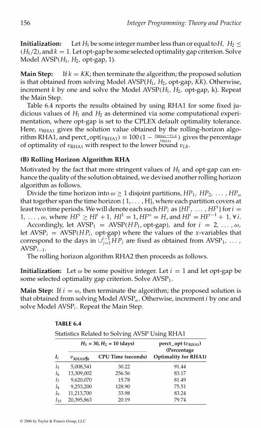
Table 6.4 reports the results obtained by using RHA1 for some fixed ju-dicious values of H1 and H2 as determined via some computational experi-mentation, where opt-gap is set to the CPLEX default optimality tolerance.Here, vRHA1 gives the solution value obtained by the rolling-horizon algo-rithm RHA1, and perct_opt(vRHA1) ≡ 100 (1 − vRHA1−vL B

vRHA1) gives the percentage

of optimality of vRHA1 with respect to the lower bound vLB.

(B) Rolling Horizon Algorithm RHA

Motivated by the fact that more stringent values of H1 and opt-gap can en-hance the quality of the solution obtained, we devised another rolling horizonalgorithm as follows.

Divide the time horizon into ω ≥ 1 disjoint partitions, HP1, HP2, . . . , HPω

that together span the time horizon 1, . . . , H, where each partition covers atleast two time periods. We will denote each such HPi as HIi , . . . , HFi for i =1, . . . , ω, where HFi ≥ HIi + 1, HI1 = 1, HFω = H, and HIi = HFi−1 + 1, ∀ i.

Accordingly, let AVSP1 = AVSP(H P1, opt-gap), and for i = 2, . . . , ω,let AVSPi = AVSP(H Pi , opt-gap) where the values of the x-variables thatcorrespond to the days in ∪i−1

j=1 H Pj are fixed as obtained from AVSP1, . . . ,AVSPi−1.

The rolling horizon algorithm RHA2 then proceeds as follows.

Initialization: Let ω be some positive integer. Let i = 1 and let opt-gap besome selected optimality gap criterion. Solve AVSP1.

Main Step: If i = ω, then terminate the algorithm; the proposed solution isthat obtained from solving Model AVSPω. Otherwise, increment i by one andsolve Model AVSPi . Repeat the Main Step.

TABLE 6.4

Statistics Related to Solving AVSP Using RHA1H1 = 30, H2 = 10 (days) perct_opt (vRHA1)

(PercentageIi vRHA1($) CPU Time (seconds) Optimality for RHA1)

I5 5,008,541 30.22 91.44I6 13,309,002 256.56 83.17I7 9,620,070 15.78 81.49I8 9,253,200 128.90 75.51I9 11,213,700 33.98 83.24I10 20,395,863 20.19 79.74


P1: shibu/Vijay

August 12, 2005 10:42 1914 1914˙C006


TABLE 6.5

Statistics Related to Solving AVSP Using RHA2CPU CPU CPU

v(AVSP1) HF1 Time v(AVSP2) HF2 Time v(AVSP3) HF3 TimeIi ($) (days) (seconds) ($) (days) (seconds) ($) (days) (seconds)

I5 4,580,000 80 0.28 4,680,000 120 47.41 N/AI6 11,069,999 80 2,501.30 11,400,000 120 0.52 N/AI7 7,840,000 80 0.61 7,900,000 120 0.83 8,000,000 150 22.14I8 7,265,000 90 0.73 7,310,000 150 860.27 7,400,000 180 1.64I9 9,335,000 90 1.61 9,339,999 170 49.89 9,360,000 210 0.95I10 16,265,333 90 2.44 16,293,333 170 34.52 16,450,000 240 5.77

Let vRHA2 denote the solution value obtained by the rolling horizon algo-rithm RHA2, and let perct_opt(vRHA2) = 100(1 − vRHA2−vL B

vRHA2), which gives the

percentage of optimality of vRHA2 with respect to the lower bound vLB. More-over, let perct_imp(vRHA2, vRHA1) = 100( vRHA1−vRHA2

vRHA1), which gives the percent-

age of improvement in total cost of algorithm RHA2 over algorithm RHA1.Table 6.5 and Table 6.6 report statistics related to algorithm RHA2, whereopt-gap is set to the default CPLEX optimality gap.

Note that the sets of test problems I5, I6, and I7, . . . , I10 were solvedusing two and three partitions, respectively. Furthermore, algorithm RHA2produced better results than RHA1 for all the test problems under consider-ation. Note that the performance of these algorithms (particularly the latter)may be enhanced by using higher-grade computers that would permit fixingor relaxing fewer variables at each step.

6.6.3 Comparison with an ad-hoc Scheduling Procedure

In this section, we compare the performance of the proposed modeling ap-proach vs. an ad-hoc scheduling procedure that represents the processadopted by Kuwait Petroleum Corporation. Since chartering expenses arelarge relative to operational costs and penalties imposed for undesirable

TABLE 6.6

Statistics Related to Solving AVSP Using RHA2perct_opt (vRHA2) perct_imp (vRHA2, vRHA1)

Total (Percentage (PercentageCPU Time Optimality Improvement of

Ii vRHA2($) (seconds) for RHA2) RHA2 over RHA1)

I5 4,680,000 47.69 97.86 6.56I6 11,400,000 2,501.82 97.10 14.34I7 8,000,000 23.58 98.00 16.84I8 7,400,000 862.64 98.17 20.02I9 9,360,000 52.45 99.73 16.53I10 16,450,000 42.73 98.87 19.34


P1: shibu/Vijay

August 12, 2005 10:42 1914 1914˙C006


storage levels, this ad-hoc procedure attempts to fully utilize company-ownedvessels before resorting to chartered vessels, and operates as follows:

(A) Examine the first day of the time horizon, say h, on which deliv-ery of shipments is possible without exceeding SL2, and dispatchcompany-owned vessels for delivery on day h so that the total stor-age level on that day will not exceed SL2. This involves exploringvarious feasible departure days, and the usage of different combi-nations of vessels. This process is repeated for the company-ownedvessels, taking into account the availability of vessels during thedays of the time horizon, until it becomes impossible to do so.

(B) Repeat Step A, however, without exceeding b2, i.e., allowing for theType I penalty when the storage level lies within (SL2, b2].

(C) Repeat Step A, however, without exceeding UB, i.e., allowing forthe Type I and Type II penalties when the storage level lies within(SL2, UB].

(D) Now, if the storage level on any given day of the horizon is not be-low zero, then we are done, and hence, there is no need for charteredvessels. Otherwise, let hh be a day when the storage level becomesnegative, and select the smallest sized vessel that is available forchartering to be dispatched for delivery on a day in (hh − δ), whereδ is to be determined by the scheduler. Repeat this step as neces-sary, however, using the already selected chartered vessel(s). At eachpass through this process, if the storage level on any given day of thetime horizon is nonnegative, then we are done. On the other hand,if there exist no more chartered vessels while for some day we stillhave a storage level below zero, then no feasible solution is found.

putational statistics for comparing schedules obtained via Procedure AH withthose generated by the proposed modeling approach. Here, vAH representsthe total cost of the solution obtained via AH and vmin gives the objective valueof the best solution obtained via the proposed modeling approach. Also, letperct_imp(vmin, vAH) = 100[( vAH−vmin

vAH)], which gives the percentage improve-

ment in the total cost of the schedules generated by the proposed modelingapproach over those obtained via the ad-hoc procedure.

Observe that for each of the test problems I1, . . . , I10, the overall cost ob-tained via the proposed modeling approach is often substantially better thanthe overall cost obtained via the ad-hoc procedure AH. For example, in testproblem I10, the improvement in total cost obtained via the modelingapproach over that obtained via the existing AH procedure is $47,090,000.Notice also that there is a large variance in the performance of the ad-hoc proce-dure AH vs. the proposed approach. The reason for this is two-fold. First,the AH procedure makes myopic decisions and is unable to recognize complexcompromises that sometimes need to be made for attaining an overall efficient


Let AH denote the foregoing ad-hoc procedure. Table 6.7 presents some com-

P1: shibu/Vijay

August 12, 2005 10:42 1914 1914˙C006


TABLE 6.7

Comparison of the ad-hoc Procedure AH vs. the ProposedModeling Approach

(Percentage Improvementof the Proposed Approach

over the Ad-hoc Approach)Ii vmin($) vAH($) perct_imp (vmin, vAH)

I1 420,000 720,000 41.66I2 660,000 720,000 8.33I3 660,000 2,480,000 73.38I4 1,500,000 3,940,000 61.93I5 4,680,000 6,720,000 30.35I6 11,400,000 42,178,000 72.97I7 8,000,000 10,880,000 26.47I8 7,400,000 8,282,000 10.65I9 9,360,000 56,450,000 83.42I10 16,450,000 24,140,000 31.85

solution. Second, because of such myopic decisions that unwisely use the self-owned vessel resources, the ad-hoc procedure often needs to resort to unneces-sary chartering of vessels, which is an expensive venture. On the other hand,the proposed modeling approach makes more effective and robust decisions.

6.7 Summary, Conclusions, and Future Research

In this chapter, we presented mixed-integer programming models for deter-mining an optimal mix of vessels of different types that are needed to transporta product from a source to a destination based on a stream of consumptionrates at the destination’s facility. Various cost components such as daily op-erational costs of vessels, chartering expenses, and penalties associated withundesirable storage levels are incorporated in the models. Such single source-destination vessel scheduling problems are faced by oil companies, for exam-ple, in which the product is crude oil, the source is a refinery facility, and thedestination is a storage location that belongs to a client. Problems of this typealso arise in practice where large quantities of crude oil need to be shippedfrom a country such as Kuwait to specific aggregated clusters of locations inEurope, North America, or Asia.

Due to the combinatorial nature of the problem, a manual scheduling ofvessels is often expensive and requires an inordinate amount of effort forconstructing and revamping vessel schedules. Therefore, it is imperative toutilize modeling approaches to advantageously compromise between thevarious cost components in order to avoid unduly high vessel charteringand penalty expenses. The proposed modeling approach enables the trans-porting organization to generate and revamp vessels’ schedules as frequently


P1: shibu/Vijay

August 12, 2005 10:42 1914 1914˙C006


as necessary and in a timely fashion. This approach also allows the organiza-tion to contemplate long-term plans regarding the size of the self-owned fleetand the need for chartered vessels.

The efficiency of the proposed modeling approach is assessed by com-paring it against an ad-hoc scheduling procedure that represents the actualscheduling of vessels in a related case study concerning Kuwait PetroleumCorporation (KPC). Using a set of ten realistic test problems, the results in-dicate that the proposed approach substantially improves upon the manualprocedure, resulting in savings ranging from $60,000 to $47,090,000.

The current manual practice at KPC suffers from a lack of robustness be-cause of the myopic nature of decisions made. Often, such decisions encumberthe self-owned vessels ineffectively, resulting in relatively large expenses forchartering additional vessels. On the other hand, the developed proceduredetermines near-optimal solutions more robustly within 97 to 99 percent ofoptimality.

This work can be extended to examine the cost effectiveness of simultane-ously investigating multiple sources and destinations instead of associatingspecific vessels with designated source-destination combinations. We can alsoexplore the impact of leasing temporary transshipment storage depots on theoverall chartering and penalty costs, whereby fewer chartered vessels mightneed to be acquired. These two extensions are the subject of a companionfollow-on paper [31].

Acknowledgments

This research work was supported by Kuwait University under ResearchGrant No. SM-06/02 and the National Science Foundation under ResearchGrant No. DMI-0094462. Special thanks to Mrs. Lulwa Al-Shebeeb forher contribution in the computational implementation of the solutionalgorithms.

References

1. Al-Yakoob, S.M., Mixed-integer mathematical programming optimization mod-els and algorithms for an oil tanker routing and scheduling problem, PhD. dis-sertation, Department of Mathematics, Virginia Polytechnic Institute and StateUniversity, Blacksburg, 1997.

2. Appelgren, L.H., A column generation algorithm for a ship scheduling problem,Transportation Science, 3, 53, 1969.

3.lem, Transportation Science, 5, 64, 1971.

4. Bausch, D.O., Brown, G.G., and Ronen, D., Scheduling short-term marine trans-port of bulk products, Maritime Policy and Management, 25(4), 335, 1998.

5. Brown, G.G., Graves, G.W., and Ronen, D., Scheduling ocean transportation ofcrude oil, Management Science, 32, 335, 1983.


Appelgren, L.H., Integer programming methods for a vessel scheduling prob-

P1: shibu/Vijay

August 12, 2005 10:42 1914 1914˙C006


6. Cho, S.C. and Perakis, A.N., Optimal liner fleet routing strategies, Maritime Policyand Management, 23(3), 249, 1996.

7. Christiansen, M., Decomposition of a combined inventory and time constrainedship routing problem, Transportation Science, 3(1), 3, 1999.

8. Christiansen, M., Fagerholt, K., and Ronen, D., Ship routing and scheduling:status and prospective, Transportation Science, 38(1), 1, 2004.

9. Datz, I.M., Fixman, C.M., Friedberg, A.W., and Lewinson, V.A., A description ofthe maritime administration mathematical simulation of ship operations, Trans.SNAME, 493, 1964.

10. Fagerholt, K., A computer-based decision support system for vessel fleetscheduling — Experience and future research, Decision Support Systems, 37(1),35, 2004.

11. Fagerholt, K. and Christiansen, M., A combined ship scheduling and allocationproblem, Journal of the Operational Research Society, 51(7), 834, 2000a.

12. Fagerholt, K. and Christiansen, M., A traveling salesman problem with alloca-tion time window and precedence constraints — an application to ship schedul-ing, International Transactions in Operational Research, 7(3), 231, 2000b.

13. Jaramillo, D.I. and Perakis, A.N., Fleet deployment optimization for liner ship-ping, Part 2: Implementation and results, Maritime Policy and Management, 18(4),235, 1991.

14. Koenigsberg, E. and Lam, R.C., Cyclic queue models of fleet operations, Opera-tions Research, 24(3),516, 1976.

15. Koenigsberg, E. and Meyers, D.A., An interacting cyclic queue model of fleetoperations, The Logistics and Transportation Review, 16, 59, 1980.

16. Lane, D.E., Heaver, T.D., and Uyeno, D., Planning and scheduling for efficiencyin liner shipping, Maritime Policy and Management, 14(2), 109, 1987.

17. Lawrence, S.A., International Sea Transport: the Years Ahead, Lexington Books,Lexington, 1972.

18. Nemhauser, G.L. and Yu, P.L., A problem in bulk service scheduling, OperationsResearch, 20, 813, 1972.

19. Perakis, A.N. and Jaramillo, D.I., Fleet deployment optimization for liner ship-ping, part 1: Background, problem formulation and solution approaches, Mar-itime Policy and Management, 18(3), 183, 1991.

20. Perakis, A.N., Fleet operations optimization and fleet deployment, in The HandBook of Maritime Economics and Business, Grammenos, C.T., Ed., Lloyds of LondonPublications, London, 2002, 580.

21. Perakis, A.N. and Bremer, W.M., An operational tanker scheduling optimizationsystem: background, current practice and model formulation, Maritime Policyand Management, 19(3), 177, 1992.

22. Powell, B.J. and Perakis, A.N., Fleet deployment optimization for liner shipping:an integer programming model, Maritime Policy and Management, 24(2), 183,1997.

23. Psaraftis, H.N., Foreword to the focused issue on maritime transportation, Trans-portation Science, 33(1), 1, 1999.

24. Rana, K. and Vickson, R.G., A model and solution algorithm for optimal routingof a time-chartered containership, Transportation Science, 22(2), 83, 1988.

25. Rana, K. and Vickson, R. G., Routing container ships using Lagrangian relax-ation and decomposition. Transportation Science, 25(3), 201, 1991.

26. Ronen, D., Cargo ships routing and scheduling: survey of models and problems,European Journal of Operational Research, 12, 119, 1983.


P1: shibu/Vijay

August 12, 2005 10:42 1914 1914˙C006


27. Ronen, D., Ship scheduling: the last decade, European Journal of Operational Re-search, 71, 325, 1993.

28. Ronen, D., Marine inventory routing: shipment planning, Journal of the Opera-tional Research Society, 53, 108, 2002.

29. Scott, J. L., A transportation model, its development and application to a shipscheduling problem, Asia-Pacific Journal of Operational Research, 12, 111, 1995.

30. Sherali, H.D., Al-Yakoob, S.M., and Merza, H., Fleet management models andalgorithms for an oil-tanker routing and scheduling problem, IIE Transactions,31, 395, 1999.

31. Sherali, H.D., Al-Yakoob, S.M. Determining an optimal fleet mix and sched-ules: Part II—multiple sources and destinations, and the option of leasing trans-shipment depots. Department of Mathematics and Computer Science, KuwaitUniversity, 2004. (Part I of the sequence is the present chapter.)

32. Xinlian, X., Tangfei, W., and Daisong, C., A dynamic model and algorithm forfleet planning, Maritime Policy and Management, 27(1), 53, 2000.

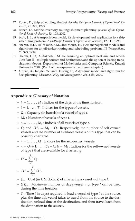
Appendix A: Glossary of Notation

• h = 1, . . . , H : Indices of the days of the time horizon.• t = 1, . . . , T : Indices for the types of vessels.• t : Capacity (in barrels) of a vessel of type t.• Mt : Number of vessels of type t.• n = 1, . . . , Mt : Indices of all vessels of type t.• Ot and CHt = Mt − Ot: Respectively, the number of self-owned

vessels and the number of available vessels of this type that can bepossibly chartered.

• n = 1, . . . , Ot : Indices for the self-owned vessels.• n = Ot + 1, . . . , Ot + CHt ≡ Mt : Indices for the self-owned vessels

of type t that are available for chartering.

• O =T∑

t=1

Ot.

• CH =T∑

t=1

CHt.

• $t,n : Cost (in U.S. dollars) of chartering a vessel n of type t.• UTt,n : Maximum number of days vessel n of type t can be used

during the time horizon.• Tt : Time ( in days) required to load a vessel of type t at the source,

plus the time this vessel takes to travel from the source to the des-tination, unload time at the destination, and then travel back fromthe destination to the source.


P1: shibu/Vijay

August 12, 2005 10:42 1914 1914˙C006


• Tt = T1,t + T2,t.

• T1,t : Time (in days) required to load a vessel of type t at the sourceand then travel to the destination.

• T2,t : Time (in days) required to unload a vessel of type t at thedestination and then travel back to the source.

• DCt,n : Daily operational cost (in U.S. dollars) of vessel n of type t.• Ct,n = T1,t (DCt,n).

• Q : A production capacity (in barrels) or certain imposed quota ofthe product at the source.

• w : Storage level (in barrels) at the destination at the beginning ofthe time horizon.

• SL1 and SL2 : The minimum and maximum desired levels (in bar-rels), respectively, at the destination’s storage facility, which shouldbe maintained to the extent possible in order to avoid penalties.

• π : Daily penalty (in U.S. dollars) for each shortage or excess unit atthe destination.

• A1 and A2 : Permitted shortage and excess quantities (in barrels) atthe destination with respect to the desired levels SL1 and SL2, re-spectively.

• b1 = SL1 − A1.

• b2 = SL2 + A2.

• UB : Upper bound on the maximum storage level (in barrels) at thedestination.

• λ : Type II penalty (in U.S. dollars).• Rj : Expected consumption rate (in barrels) at the destination on

day j , for j = 1, . . . , H.

• TCh =h∑

j=1

Rj .

• Sh : A continuous variable representing the storage level on day h.• PI (Sh) = π maximum 0, (SL1 − Sh), (Sh − SL2) if Sh ∈ [b1, b2].

• PI I (Sh) =

π A1 + λ (b1 − Sh) if Sh ∈ (0, b1)

π A2 + λ (Sh − b2) if Sh ∈ (b2, U B).

• Sh = S1,h − S2,h − S3,h + S4,h + S5,h ,

where SL1 ≤ S1,h ≤ SL2, 0 ≤ S2,h ≤ A1, 0 ≤ S3,h ≤ b1,0 ≤ S4,h ≤ A2, and 0 ≤ S5,h ≤ U B − b2.

• P(Sh) = π(S2,h + S4,h) + λ(S3,h + S5,h).

• Xh,t,n =

1 if vessel n of type t departs the source towardthe destination on day h,

0 otherwise.


P1: shibu/Vijay

August 12, 2005 10:42 1914 1914˙C006


• Yh,t,n =

1 if vessel n of type t is available at the source on day h,

0 otherwise.

• Zt,n =

1 if vessel n of type t is selected for chartering during(all or only part of) the time horizon,

0 otherwise.• φX and φY : Sets of X and Y variables, respectively, that are restricted

to be fixed at specified binary values by virtue of such considera-tions.

• DCt : Average daily operational cost (in U.S. dollars) of a vessel oftype t.

• Ct = Tt (DCt).

• xh,t : An integer variable that represents the number of vessels oftype t that are dispatched from the source on day h.

• yh,t : An integer decision variable that represents the maximumnumber of vessels of type t that are available for dispatching fromthe source on day h.

• Oh,t : Number of vessels of type t that will become available for useat the source for the first time on day h of the time horizons.

• CHh,t : Number of vessels of type t that will become available forchartering on day h of the time horizon.

• αh,t = Oh,t + CHh,t : Number of vessels of type t that will becomeavailable for use on day h of the time horizon.

• Ot =∑

h

Oh,t.

• C Ht =∑

h

CHh,t.

• zh,t : An integer variable that denotes the number of vessels oftype t that are actually selected for chartering on day h of the timehorizon.

• $h,t : Average chartering cost (in U.S. dollars) of a vessel of type tthat will become available for use on day h of the time horizon.

• Ah,t : A subset of indices for the vessels of type t (both self-ownedand vessels available for chartering) that will become available foruse at the source for the first time on day h of the time horizon.

• UTh,t =∑

n∈Ah,tUTt,n

αh,t, which basically gives the average usage allow-

ance (in days) for a vessel of type t that will become available foruse for the first time on day h of the time horizon.

• φx and φy : Sets of x- and y-variables, respectively, that are a pri-ori restricted to be zero, or fixed at some known positive integervalue.


P1: shibu/Vijay

August 12, 2005 10:42 1914 1914˙C006


• P : Linear relaxation of any model P .• v(P) : Optimal objective function value of model P .• vU B(P) : Best upper bound (solution) found for model P .• vL B(P) : Best lower bound found for model P .• Ii : Test problem i , for i = 1, . . . , 10.

• “•”: Indicate that no meaningful solution of a given model is ob-tained by a direct application of CPLEX due to out-of-memorydifficulties.

• AVSP(H, opt-gap) : Relaxation of Model AVSP for which integralityis enforced only on the pertinent x-variables that correspond to day1 through day H of the time horizon, and an optimal solution isrequired to be found within a tolerance “opt-gap” of optimality.

• RHA1 and RHA2 : Rolling horizon algorithms.• vRHA1 : Solution value (in U.S. dollars) obtained by RHA1.

• perct_opt(vRHA1) ≡ 100(

1 − vRHA1−vL BvRHA1

)• vRHA2 : Solution value (in U.S. dollars) obtained by RHA2.

• perct_opt(vRHA2) = 100(

1 − vRHA2−vL BvRHA2

).

• perct_imp(vRHA2, vRHA1) = 100(

vRHA1−vRHA2vRHA1

).

• AH: The ad-hoc procedure.• vAH : Total cost (in U.S. dollars) obtained via AH.• vmin : Objective value (in U.S. dollars) of the best solution obtained

via the proposed modeling approach.

• perct_imp(vmin, vAH) = 100[(

vAH−vminvAH

)].

Appendix B: Test Problems

This appendix presents statistics related to ten test problems. Assume thatthere are four vessel types. Note that the models described in this chapter

TABLE B.1

Vessel Typest Ωt (barrels) $t($) DCt($)

1 400,000 3,000,000 6,0002 600,000 4,000,000 8,0003 800,000 5,500,000 10,0004 1,200,000 7,000,000 13,500


P1: shibu/Vijay

August 12, 2005 10:42 1914 1914˙C006


TABLE B.2

Test ProblemsT (vessel (O1, O2, O3, O4) (CH1, CH2, CH3, CH4) (T1, T2, T3, T4)

Ii H (days) types) (vessels) (vessels) (days) w (barrels)

I1 30 1 (4,0,0,0) (5,0,0,0) (10,0,0,0) 4,000,000I2 60 1 (2,0,0,0) (2,0,0,0) (10,0,0,0) 7,000,000I3 60 2 (2,3,0,0) (2,7,0,0) (10,20,0,0) 7,000,000I4 90 2 (2,2,0,0) (2,3,0,0) (10,20,0,0) 7,000,000I5 120 2 (3,4,0,0) (8,7,0,0) (20,30,0,0) 7,000,000I6 120 4 (1,1,1,1) (3,4,2,6) (20,30,40,50) 7,000,000I7 150 3 (2,5,2,0) (1,5,2,0) (20,30,40,0) 4,000,000I8 180 3 (5,1,6,0) (2,7,9,0) (20,30,40,0) 7,000,000I9 210 4 (4,2,1,4) (3,2,1,4) (20,30,40,50) 7,000,000I10 240 4 (5,2,2,2) (1,2,2,6) (30,40,50,60) 7,000,000

consider a single source-destination operation. We assume that the dailyconsumption rate for a given destination is the same for the duration of agiven time-horizon (denoted by R1), and that the daily operational costs ofvessels of a given type are also the same. The Type I penalty is fixed at $3and the Type II penalty is fixed at $500. Specific details for the test problems

of ten test problems. Note that R1 = 150, 000, SL1 = 2, 250, 000, SL2 =10, 000, 000, and A1 = A2 = 1, 000, 000 for all the test problems. Also, notethat Ti = 0 indicates that no vessels of type i are involved in the operation.


are presented in Table B.1 and Table B.2, where Table B.2 describes our set

1914ch6

Documents

Transcript of 1914ch6