17

3. Train Control and Signaling

3.1 INTRODUCTION

Signaling has been a feature of urban rail transit from theearliest days. Its function is to safely separate trains from eachother. This includes both a separation between following trainsand the protection of specific paths through junctions and cross-overs. The facilities that create and protect these paths or routesare known as interlockings.

Additional functions have been added to basic signaling,starting, again from a very early date, with automatic train stops.These apply the brakes should a train run through a stop signal.Speed control can also be added, usually to protect approachesto junctions (turnouts), sharp curves between stations andapproaches to terminal stations where tracks end at a solid wall.Automatic trains stops are in universal use. Speed control is amore recent and less common application, often introduced inconjunction with automatic train control or to meet specificsafety concerns.

Rail transit signaling is a very conservative field maintaininghigh levels of safety based on brick-wall stops and fail-safeprinciples. A brick-wall stop means that the signaling separationprotects a train even if it were to stop dead, an unlikely thoughpossible event should a train derail and strike a structure. Thisprotection allows for a) the following train’s failure to observe astop signal, b) driver and equipment reaction time, and c) someimpairment in the braking rate.

Fail-safe design principles ensure that failure of single—andoften multiple—components should never allow an unsafeevent. Traditionally in North America this involves the use ofheavy railroad style relays that open by gravity and havenonwelding carbon contacts. Compact, spring opening,European-style relays or solid state (electronic or computercontrolled) interlockings are now being accepted. Hereequivalent safety is provided by additional logic, duplicatecontacts or multiple polling processors.

The rigor with which fail-safe principles have been applied torail transit has resulted in an exceptional safety record.However, the safety principles do not protect against allpossibilities—for example, a derailed train could interfere withthe safe passage of a train on an adjacent parallel track. Nor dothey protect against all possible human errors whether caused bya signal maintainer, dispatcher or train driver. An increasinginability to control the human element—responsible for three-quarters of rail transit accidents or incidents1—has resulted innew train control systems using technology or automation toreduce or remove the possibility of human error.

Train control, or more properly automatic train control, addsfurther features to basic signaling. Automatic train control is anill-defined term but usually encompasses three levels:

1 PARKINSON, TOM, Safety Issues Associated with the Implementation of

ATCS-Type Systems, Transportation Development Centre, TransportCanada, August 1989.

• Automatic train protection (ATP)• Automatic train control2 (ATC or ATO)• Automatic train supervision (ATS)

Automatic train protection is the basic separation of trains andprotection at interlockings. In other words, the signaling systemas described above.

Automatic train control adds speed control and oftenautomatic train operation. This can extend to automaticallydriven trains but more commonly includes a driver, operator orattendant who controls the train doors and observes the trackahead.

Automatic train supervision attempts to regulate train service.It can be an integral feature of automatic train control or anaddon system. The capabilities of automatic train supervisionvary widely from little more than a system that reports thelocation of trains to a central control office, to an intelligentsystem that automatically adjusts the performance and stoptimes of trains to maintain either a timetable or an even headwayspacing.

Automatic train protection and automatic train controlmaintain the fail-safe principles of signaling and are referred toas vital or safety critical systems. Automatic train supervisioncannot override the safety features of these two systems, and soit is not a vital system.

This chapter describes and compares the separationcapabilities of various train control systems used on or beingdeveloped for rail transit. It is applicable to the main rail transitgrouping of electrically propelled, multiple-unit, grade-separated systems. Specific details of train control for commuterrail and light rail modes are contained in the chapters dealingwith these modes.

These descriptions cannot include all the complexities andnuances of train control and signaling but are limited to theireffect on capacity. More details can be found in the referencesand in the bibliography. All urban rail transit train controlsystems are based on dividing the track into blocks and ensuringthat trains are separated by a suitable and safe number of blocks.Train control systems are then broken down into fixed-blockand moving-block signaling systems.

3.2 FIXED-BLOCK SYSTEMSIn a fixed-block system, trains are detected by the wheels andaxles of a train shorting a low-voltage current inserted into therails. The rails are electrically divided into blocks. Originallythis required a rail to be cut and an insulating joint inserted.Only one rail is so divided. The other rail remains continuous tohandle the traction power return.

2 Sometimes termed automatic train operation to avoid confusion with the

overall term automatic train control.

18

By moving from direct current to alternating current circuits,3

the blocks can be divided by an inductive shunt4 connectedacross the rails, avoiding the need for insulated joints. These arecalled jointless track circuits and both rails are then available fortraction power return. A track circuit can be any reasonablelength. Each circuit is expensive so lines use the minimumrequired for appropriate headways. Circuits will be short wheretrains must be close together, for example in a station approach,and can be longer between stations where trains operate at speed.

The signaling system knows the position of a train only by therelatively coarse measure of block occupancy. It does not knowthe position of the train within the block; it may have only afraction of the train, front or rear, within the block. At blockboundaries, the train will occupy two blocks simultaneously fora short time.

In the simplest two-aspect block system, the signals displayonly stop (red) or go (green). A minimum of two empty blocksmust separate trains, and these blocks must be long enough forthe braking distance plus a safety distance. The safety distancecan include several components, including sighting distances,driver and equipment reaction times, and an allowance forpartial brake failure, i.e. a lower braking rate.

Automatic train stops have long been a feature of rail transit(almost from the turn of the century). These prevent a trainrunning through a red signal by automatically applying theemergency brakes should the driver ignore a signal. Called a tripstop, the system consists of a short mechanical arm beside theouter running rail that is pneumatically or electrically raisedwhen the adjacent signal shows a stop aspect. If a train runsthrough this signal, the raised arm strikes and actuates a tripcock on the train that evacuates the main air brake pipe. Fullemergency braking is then applied along the length of the train.To reset the trip cock the driver must usually climb down totrack side and manually close the air valve.5

A two-aspect signaling system does not provide the capacitynormally required on busy rail transit lines—those with trains an

3 Alternating current track circuits use different frequencies, combinations of

frequencies or modulated frequencies. In all cases care must be taken toavoid interference from on-board vehicle equipment. Modern high powerchopper and VVVF (variable voltage, variable frequency) three phase acmotor control equipment can emit considerable levels of EMI (electromagnetic interference). The systems engineering to coordinate and avoidsuch interference is difficult and complex and is beyond the scope of thisreport.

4 In essence, the shunt shorts the small alternating current track circuitswhile presenting a low resistance to the high direct currents.

5 Resetting the trip cock is understandably an unpopular task and consumestime. Consequently drivers may approach a trip cock cautiously at lessthan the optimal speed, particularly when closely following another train.In this case they expect the signal aspect to change as they approach butcannot be certain. Automatically driven trains will typically operate closerto the optimal speeds and braking rates and so can increase throughput.

There are times when it is operationally desirable to operate through astop signal and its associated automatic train stop, particularly when thetrain ahead is delayed in a station and following trains wish to close up toexpedite their subsequent entry to the station. The process is commonlycalled key by from an arrangement where the driver must lean out of thecab and insert a key in an adjacent electrical switch. However, the mostcommon arrangement no longer involves a key, merely a slow movementof the train into the next block, which lowers the trip stop before it isstruck by the train. The train must then proceed on visual rules toward thetrain ahead. In recent years an increase in the number of incidents causedby this useful, time saving, but not fail-safe, procedure has caused severalsystems to prohibit or restrict its use.

hour or better. Increased capacity can be obtained from multipleaspects where intermediate signals advise the driver of thecondition of the signal ahead, so allowing a speed reductionbefore approaching a stop signal. Block lengths can be reducedrelative to the lower speed, providing increased capacity.

The increased number of blocks, and their associated relaycontrols and color-light signals, is expensive. There is adiminishing capacity return from increasing the number ofblocks and aspects as shown in Figure 3.1. This figure alsoshows that there is an optimal speed to maximize capacity.Between stations the line capacity is greatest with maximumrunning speeds of between 40 km/h (25 mph) with three aspectsto 55 km/h (34 mph) with 10 aspects. At the station entry—invariably the critical point for maximum throughput—optimalapproach speeds are from 25 km/h (15 mph) to 35 km/h (22mph).

In North America, the most common block signalingarrangement uses three aspects. In Europe and Japan, a smallnumber of systems extend to four or five aspects.

Optimizing a fixed-block system is a fine art, with respectboth to block lengths and to boundaries. Block lengths are alsoinfluenced by grades because a train’s braking distanceincreases on a down grade and vice-versa. Grades down into astation and curves or special work with significant speedrestrictions, below the optimal levels given above, will reducethroughput and so reduce capacity. Fortuitously, one usefuldesign feature of below-grade systems is a gravity-assistedprofile. Here the stations are higher than the general level of therunning tunnel. Trains use gravity to reduce their brakingrequirements in the station approach and to assist themaccelerating away from the stations. This not only reducesenergy consumption, equipment wear and tear and tunnelheating, but also reduces station costs because they are closer tothe surface, allowing escalators and elevators to be shorter.More important to this study, it increases train throughput—altogether a good thing.

Requiring a train operator to control a train’s speed andcommence braking according to multiple aspect color-lightsignaling requires considerable precision to maximizethroughput. Coupled with the expense of increasing the numberof aspects an improvement has been developed over the pastthree decades—cab signaling.

Figure 3.1 Throughput versus number of signal aspects(R26)

19

3.2.1 CAB SIGNALING

Cab signaling uses a.c. track circuits such that a code is insertedinto each circuit and detected by an antenna on each train. Thecode specifies the maximum allowable speed for the blockoccupied and may be termed the reference or authorized speed.This speed is displayed in the driver’s cab—typically on a dualconcentric speedometer, or a bar graph where the authorizedspeed and actual speed can be seen together.

The authorized speed can change while a train is in a block asthe train ahead proceeds. Compared to color-light signals, thedriver can more easily adjust train speed close to the optimumand has less concern about overrunning a trip stop. Problemswith signal visibility on curves and in inclement weather arereduced or eliminated.

Cab signaling avoids much of the high capital andmaintenance costs of multiple-aspect color-light signals,although it is prudent and usual to leave signals at interlockingsand occasionally on the final approach to and exit from eachstation. In some situations, dwarf color-light signals can be used.In this way trains or maintenance vehicles that are not equippedwith cab signaling—or trains with defective cab signaling—cancontinue to operate, albeit at reduced throughput.

Reducing the number of color-light signals makes iteconomically feasible to increase the number of aspects and it istypical, although not universal, to have the equivalent of fiveaspects on a cab-signaling system. A typical selection ofreference speeds would be 80, 70, 50, 35 and 0 km/h (50, 43,31, 22 and 0 mph).

Signal engineers may argue over the merits of block-signalingand cab-signaling equipment from various manufacturers—particularly with respect to capital and maintenance costs,modular designs, plug versus hard-wired connections and thecomputer simulation available from each maker to optimizesystem design. However, for a given specification, thethroughput capabilities vary little provided that—the signaling isoptimized as to block length, boundary positioning and, whenapplicable, the selection of reference speeds. Consequently alisting or description of different systems is not relevant tocapacity determination.

3.3 MOVING-BLOCKSIGNALING SYSTEMSMoving-block signaling systems are also called transmission-based or communication-based signaling systems—potentiallymisleading because cab signaling is also transmission based.

A moving-block signaling system can be likened to a fixed-block system with very small blocks and a large number ofaspects. Several analytic approaches to moving-block systemsuse this analogy. However a moving-block signaling system hasneither blocks nor aspects. The system is based on a continuousor frequent calculation of the clear (safe) distance ahead of eachtrain and then relaying the appropriate speed, braking oracceleration rate to each train.

This requires a continuous or frequent two-waycommunication with each train, and a precise knowledge of atrain’s location, speed and length; and fixed details of the line—

curves, grades, interlockings and stations. These may becontained in a table that allows changes to be made without thenormal full rigor required for changes to safety-critical software.Temporary changes can be easily made to add speed restrictionsor close off a section of track for maintenance work.

Based on this information, a computer can calculate the nextstopping point of each train—often referred to as the targetpoint—and command the train to brake, accelerate or coastaccordingly. The target point will be based on the normalbraking distance for that train plus a safety distance.

Safety Distance Braking distance is a readily determined orcalculated figure for any system. The safety distance is lesstangible because it includes a calculated component adjusted byagency policy. In certain systems this distance is fixed;however, the maximum throughput is obtained by varying thesafety distance with speed and location—and, where differenttypes of equipment are operated, by equipment type.

In theory, the safety distance is the maximum distance a traincan travel after it has failed to act on a brake command beforeautomatic override (or overspeed) systems implementemergency braking. Factors in this calculation include

• system reaction time;• brake actuation time;• speed;• train load (mass)—including any ice and snow load;• grade;• maximum tail winds (if applicable);• emergency braking rate;• normal braking rate;• train to track adhesion; and• an allowance for partial failure of the braking system.

The safety distance is frequently referred to as the “worst-case”braking distance, but this terminology is misleading. The trulyworst case would be a total braking failure. Worst case impliesreasonable failure situations, and total brake failure is notregarded as a realistic scenario on modern rail transit equipmentthat has multiple braking systems. A typical interpretation of thesafety distance assumes that the braking system is three-quarterseffective.

Train Position and Communication Without track circuits todetermine block occupancy, a moving-block signaling systemmust have an independent method to accurately locate theposition of the front of a train, then use look-up tables tocalculate its end position from the length associated with thatparticular train’s identification. The first moving-block systems,developed in Germany, France and the United States, all usedthe same principle—a wire laid alongside or between therunning rails periodically transposed from side-to-side, thezigzag or Grecian square arrangement. The wire also serves totransmit signals to and from antennas on the train.

The wayside wires are arranged in loops so that each trainentering a loop has a precise position. Within the loop, the controlsystem counts the number of transpositions traversed, each a

20

fixed distance apart— m (82 ft) is typical although much shorterdistances have been used. Between the transpositions, distanceis measured with a tachometer.6

The resultant positioning accuracy can be in the order ofcentimeters and with frequent braking rate feedback can resultin station stop accuracy within ± 20 cm (8 in.) or better.

The use of exposed wayside wires is abhorred bymaintenance-of-way engineers, and recent developmentsportend changes to existing systems and for the many moving-block signaling systems now under development. Inerttransponders can be located periodically along the track. Theserequire neither power nor communication wiring. They areinterrogated by a radio signal from each train and return adiscrete location code. Positioning between transponders againrelies on the use of a tachometer. Moving-block signalingsystems already have significantly lower costs for waysideequipment than do fixed-block systems, and this arrangementfurther reduces this cost as well as the occupancy time requiredto install or retrofit the equipment—an often critical factor inresignaling existing systems.

Removing the positioning and communicating wire from thewayside requires an alternate communication system. This canmost economically be provided by a radio system using over-the-air transmission, wayside radiating cables, intermittentbeacons or a combination thereof.

As with any radio system, interruption or interference withcommunications can occur and must be accommodated. Afterthe central control computer has determined any control action,it will transmit instructions to a specific train using theidentification number of the train’s communication system. It isclearly vital that these instructions are received by and only bythe train they were determined for.

There are numerous protocols and/or procedures that providea high level of security on communication systems. The datatransmission can contain both destination codes and error codes.A transmission can be received and repeated back to the sourceto verify both correct reception and correct destination, a similarprocess to radio train order dispatching. If a train does notreceive a correctly coded confirmation or command within a settime, the emergency brakes will be automatically applied. Thedistance a train may travel in this time interval—typically lessthan 3 sec—is a factor in the safety distance.

Data Processing The computers that calculate and control amoving-block signaling system can be located on each train, at acentral control office, dispersed along the wayside or acombination of these. The most common arrangement is acombination of on-board and central control office locations.

The first moving-block signaling systems used mainframecomputers with a complex interconnection system that providedhigh levels of reliability. There is now a move toward the use ofmuch less expensive and space-consuming personal computers(PCs).

6 Tachometer accuracy is helped by the ability for continual on-the-fly

calibrations as the distance between each transposition is fixed andknown. This fully compensates for wheel wear but not for slip or slide.Errors so caused, while small, can be minimized by the use of currentsophisticated slip-slide control or, where feasible, placing the tachometeron an unmotored axle.

PCs and their local area networks (LANs) have been regardedas less robust than mainframe systems, and as suspect for use insafety-critical applications. The first major application occurredin Vancouver in 1994 when, after 10 years of mainframeoperation, the entire SkyTrain train control system was changedto operating on PCs with Intel 486 CPUs. Reliability hasincreased in the subsequent 15 months of operation. However, itis not possible to attribute this improvement solely to the newhardware because new software was also required by the changein operating systems. The proprietary computers and softwareon each train were not changed.

Safety Issues Safety on rail transit is a relative matter. Itencompasses all aspects of design, maintenance and operations.In fixed-block signaling, electrical interlockings, switch andsignal setting are controlled by relay logic. A rigorous disciplinehas been built around this long established technology which theuse of processor-based controls is now infiltrating.

A moving-block signaling system is inherently processorcontrolled. Processor-based train control systems intrinsicallycannot meet the fail-safe conventions of traditional signaling.Computers, microprocessors and solid-state components havemultiple failure opportunities and cannot be analyzed and testedin the same way as conventional equipment.

Instead, an equivalent level of safety is provided on the basisof statistical failure modes of the equipment. Failure analysis isnot an exact science. Although not all failure modes can bedetermined, the statistical probability of an unsafe event7 can bepredicted.

Determining failure probability is part of a safety assuranceplan—a systematic and integrated series of performance,verification, audit, and review activities, including operations,maintenance and management activities that are implemented toassure safe and satisfactory performance. The plan can cover aspecific area, such as software, or can encompass the entiresystem, where software would be but one aspect. Such a planwill usually include a fault tree analysis.

The typical goal in designing processor-based systems is amean time between unsafe failures of 109 hours, or some114,000 years.8 After due allowance for statistical errors and theincorporation of a large safety margin, this is deemed to beequivalent to or better than the so-called fail-safe conventionalequipment.

The possibility of even a low incidence of unsafe failure maygive cause for concern and the acceptance of processor-basedsignaling, particularly moving-block systems, has been slow.However the safety of conventional rail transit signaling is notas absolute as is often made out. Minor maintenance errors cancause unsafe events. An estimated three-quarters of rail transitaccidents are attributed to human error.9

Two methods are used to achieve the high levels of safety onprocessor-based control systems. One is based on redundancy,where two or more computers operate with the same software.The output of both or the output of at least two out of three

7 An unsafe event may be referred to as a wrong-side failure.8 PARKINSON, TOM, Safety Issues Associated with the Implementation of

ATCS-Type Systems, Transportation Development Centre, TransportCanada August 1989.

9 Ibid.

21

must coincide before a comparator circuit transmits a command.Thereafter, the safety consequences of the output can beconsidered in a conventional fashion. This method is ahardware-intensive solution.

The other method is based on diversity. Two sets of software,created and verified by independent teams, are run on the sameor separate computers. Again their output must agree before anycommands are executed. This is a software-intensive solution.

Because software development can account for over half thecost of a moving-block signaling system, and with hardwarecosts declining—particularly with the use of PCs—thehardware-intensive approach to redundancy is invariably themost economic. However, the relative cost of softwaredevelopment, testing, commissioning and safety assessment isexpected to drop with the introduction of modular codeblocks—safety critical portions of software that remainunchanged from system to system.

In some regards, software-based systems, once fully testedand commissioned, are less prone to unsafe errors created duringequipment installation and maintenance. However there arethree major remaining areas of concern.

1. Revisions to software may be required from time to timeand can escape the full rigor of a safety assurance plan.

2. Removing track circuits also removes broken raildetection. While no specific data for rail transit have beenfound, the Southern Pacific Railroad found that fewer than2 percent10 of broken rails were detected in advance bytrack circuits—it appears that most breaks occur from thestress of a train passing. Nevertheless, some moving-blocksignaling systems have long track circuits added to detectbroken rails.

3. Removing track circuits also eliminates the detection ofany and all vehicles whose wheels and axles short acrossthe rails. A major hazard exists if maintenance vehicles, ora train with a defective train control system, enter into orremain in an area where automatically controlled trains arerun. This requires a rigorous application of operating rulesand requires the defect correction and reentry into thecontrol system or removal of an automatic train protectionfailed train, before service can resume in the occupiedarea.

This potential hazard can be reduced by adding axlecounters at various locations. These count entry and exitinto a specified track section. In conjunction withappropriate software, they will prevent an automated trainfrom following an unequipped train at an unsafe distance.However, an unequipped train is not so protected butdepends on the driver obeying rules, whether using line-of-sight operation, or depending on any remaining waysidesignals.

Hybrid Systems There are times when an urban rail transitsystem shares tracks with other services, such as long distancetrains, whose equipment is impractical or uneconomic to equipwith the moving-block signaling system. Use of axle countersfor the safety of unequipped rolling stock substantially reduces

10 Ibid.

capacity. To avoid this reduction while still obtaining the closeheadway of the moving-block system for the urban or shortdistance trains requires a hybrid design.

The SACEM system developed by Matra is employed in Parisand Mexico City11 The SACEM combines a fixed-block systemwith a transmission based system. Conventional blocks aresubdivided into smaller increments that permit those trains,equipped with a continuous communication system, to operateon closer headways. Unequipped trains continue to be protectedby the basic block system. As equipped trains operate throughsome signals displaying red an additional aspect must be addedto such signals—indicating that the signal is not applicable tothat specific train.

SACEM has a throughput capability between fixed-block andmoving-block signaling systems that depends on the mix ofequipped and unequipped trains. The manufacturer claims anincrease in capacity up to 25%, which is comparable to thegeneral 30% increase of moving-block over fixed-blocksignaling systems—all else being equal. The two equipped railtransit lines in Mexico City do not have any unequipped longdistance trains with their longer braking distances and so shouldobtain the maximum capacity improvement.

While classed as a hybrid system, SACEM does not usemoving-blocks and is really an overlay system. Shorter blocks—applicable to certain trains only—are overlaid onto aconventional fixed-block system.

Moving-block signaling systems have been installed by the SEL(Standard Electrik Lorenz) of Stuttgart, Germany, and itsCanadian subsidiary SEL Canada. Both are now part of theAlcatel group, a French consortium.

The Alcatel SelTrac TM system has evolved through fivegenerations over two decades. There are some 20 worldwideinstallations of which five are in North America: Vancouver,Toronto, Detroit, San Francisco and Orlando (Disneyworldmonorail).

The SelTrac system uses an inductive loop to bothcommunicate with trains and, through the loop transpositions, todetermine positioning. Processing power is centralized with theon-board computers limited to processing signals andcontrolling the vehicle subsystems. The use of Intel x86processors to control critical train movements was introduced in1994. Transponder positioning has been developed to reducehardware costs and improve failure management. In addition,SelTrac includes an integrated automatic train supervisionsubsystem.

The second manufacturer with a system in service is alsoFrench. Service started on Line D of the Lyon metro in 1992using Matra Transport’s Maggaly TM system. The Maggalysystem uses inductive transmission with positioningtransponders and places the bulk of the processing power on-board. Line data are stored on-board with the waysideequipment limited to system management and providing thelocation of a leading train to its immediate follower.

The advantages of moving-block signaling systems areconsiderable. Beyond the capacity increase of interest to thisstudy, the concept offers the potential for lower capital andmaintenance costs, flexibility, comprehensive system manag-ement capabilities and inherent bi-directional operation. The

11 Line A and Line 8.

22

slow acceptance of processor based train control systems mayexplain why most conventional train control suppliers havestayed away from this concept until the recent selection ofmoving-block systems by London Transport and New York CityTransit, together with several smaller systems. This selection isnot necessarily based on the capacity increases but as much onthe economics and relative ease of installing the system on topof a conventional signaling system on existing lines that mustremain in operation throughout the conversion, modernization orreplacement.

Subsequent to the London and New York decisions, manymanufacturers have announced the development of moving-block signaling systems.

General Railway Signal is developing its ATLAS TM system.This is a modular based concept that allows various forms ofvehicle location and communication systems. A feature is a vitalstored database and low requirements for the vehicle-waysidedata communication flow.

Union Switch & Signal is developing its MicroBlok TM

which shares some similarity with Matra’s SACEM, overlaying“virtual” software based blocks on a conventional fixed blocksystem. With radio based communications and vital logicdistributed on the wayside, the system uses some conceptsdeveloped for the Los Angeles Green Line which enteredservice in August 1995.

AEG Transportation System’s Flexiblok TM shares somefeatures with MicroBlok and SACEM. It is a radio-based systemdesigned for both standalone use and for incrementally addingcapacity and features to traditional train control systems.Operational and safety responsibilities are distributed throughthe system, which incorporates nonproprietary interfacesconforming to Open System Interconnect protocol standards.12

AEG’s US division, previously Westinghouse ElectricTransportation Systems, is developing a transmission-basedtrain control system tailored to the North American market.

Harmon Industries’ UltraBlock TM system is radio basedwith transponder positioning technology. Line profileinformation is stored on-board. Vital processing is distributedalong the wayside.

Siemens Transportation Systems is developing a moving-block system based on its Dortmund University people mover,an under-hanging cabin system that has been in service since1984.

CMW (Odebretch Group, Brazil) is supplying a radio-basedoverlay system to the São Paulo metro with distributedprocessing. The system is claimed to reduce headways from 90to 66 sec. As section 4.7 of this chapter shows, such closeheadways are only possible with tightly controlled station dwellswhich are rarely achievable at heavy volume stations.

Morrison Knudsen (with Hughes and BART) is developing amoving-block signaling system based on militarycommunication technology. The system uses beacon-based,ranging spread spectrum, radio communications which are lesssusceptible to interference and can tolerate the failure or loss ofone or more beacons.

12 The proprietary nature of many moving-block signaling systems is a

concern to potential customers who are then captive to a particularsupplier. Traditional train control systems in theory allow manycomponents from different manufacturers to be mixed and matched.However, particularly with the introduction of solid state interlockings,this is not always feasible.

NOTE: The above discussion represents the best informationavailable to the researchers at the time this report was written.Other suppliers may exist and omissions were inadvertent. Thisdiscussion is not intended to endorse specific products ormanufacturers.

All moving-block systems that base train separationon a continually adjusted distance to the next stop ortrain ahead (plus a safety distance) should havesubstantially similar train throughput capabilities.Capacity for a generic moving-block signaling systemis developed in section 3.8 of this chapter, based oninformation from existing systems (Alcatel andMatra).

Those systems under development (above) thatsucceed in the market can reasonably be expected tohave comparable capacities. However, there isinsufficient information to confirm this.

3.4 AUTOMATIC TRAINOPERATIONAutomatic acceleration has long been a feature of rail transit. Adriver no longer has to cautiously advance the control handlefrom notch to notch to avoid pulling too much current and sotripping the line breaker. Rather, relays, and more recentlymicro-processors, control the rate of acceleration smoothly fromthe initial start to maximum speed.

Cab signaling and moving-block signaling systems transferspeed commands to the train and it was a modest step to linkthese to the automatic acceleration features, and comparablecontrolled braking, to create full automatic train operation(ATO). The first North America application occurred in 1962 onNYCTA’s Times Square Shuttle, followed in 1967 byMontreal’s Expo Express, then, in short order by PATCO’sLindenwold line and San Francisco’s BART. Most new railtransit systems have incorporated ATO since this innovativeperiod.

The driver’s or attendant’s role is not necessarily limited toclosing the doors, pressing a train start button and observing theline ahead. Drivers are usually trained in, and rolling stock isprovided with, manual operating capabilities. PATCO pioneeredthe concept of having drivers take over manual control fromtime to time to retain familiarity with operations. Manualdriving under cab controls, limited color-light signaling or radiodispatching is routine, if infrequent, on many ATO-equippedsystems when there is a train control failure or to providesignaling maintenance time.

Dispensing entirely with a driver or attendant is controversial.In 1965 the driverless Transit Expressway was first operated in acontrolled environment in Pittsburgh. This Automated GuidewayTransit (AGT) system, and similar designs, have gained wide-spread acceptance in nontransit usage as driverless peoplemovers in airports, amusement parks and institutional settings.Morgantown’s AGT was the first public transit operation to gainacceptance for driverless operation when it opened in 1968. Aftera long gap Miami’s downtown people mover opened in 1985with the Detroit People Mover and the full-scale urban rail transit

23

SkyTrain system in Vancouver starting the following year.Driverless public transport is now well established in these citiesbut no subsequent operations have chosen to follow, despitetheir record of safety, reliability and lower operating costs.Fundamental concerns with driverless automatic train operationclearly remain.

Automatic train operation, with or without attendants ordrivers, allows a train to more closely follow the optimum speedenvelope and commence braking for the final station approachat the last possible moment. This reduces station to station traveltimes, and more important from the point of capacity, itminimizes the critical station close-in time—the time from whenone train starts to leave a station until the following train isberthed in that station.

In the literature Klopotov(R32) makes claims of capacityimprovements of up to 15% with ATO. Bardaji(R10) claims a 5%capacity increase with automatic regulation. Other reports alludeto increases without specific figures. None of the reportssubstantiate any claims. Attempts to quantify timeimprovements between manual and automatic driving for thisstudy were unsuccessful. Any differences were overshadowedby other variations between systems.

Intuitively there should be an improvement in the order of 5to 10% in the station approach time. As this time representsapproximately 40% of station headway, the increase in capacityshould be from 2 to 4%.

The calculations used to determine the minimum stationheadway assume optimal driving but insert a time for a driverssighting and reaction time—in addition to the equipmentreaction time. The calculations in this report compensate forATO by removing the reaction times associated with manualdriving.

3.5 AUTOMATIC TRAINSUPERVISION

Automatic Train Supervision (ATS) encompasses a wide varietyof options. It is generally not a safety-critical aspect of the traincontrol system and may not need the rigor of design and testingto its hardware and software that characterizes other areas oftrain control. At its simplest it does little more than display thelocation of trains on a mimic board or video screen in the centralcontrol or dispatcher’s office.

One step up in sophistication provides an indication of on-time performance with varying degrees of lateness designatedfor each train, possibly grouped by a color code or with a digitaldisplay of the time a train is behind schedule. In either casecorrective action is in the hands of the variously namedcontroller, dispatcher or trainmaster.

Urban rail transit in North America is generally run to atimetable. Those systems in Europe that consistently operate atthe closest headways (down to 90 sec) generally use headwayregulation that attempts to ensure even spacing of trains ratherthan adhere strictly to a timetable. Although it appears thatkeeping even headways reliably provides more capacity, this is

an issue of tradition, operating rules and safety13 that is beyondthe scope of this study.

In more advanced systems where there is ATO, computeralgorithms are used to attempt to automatically correct lateness.These are rare in North America and are generally associatedwith the newer moving-block signaling systems.

Corrective action can include eliminating coasting, increasingline speed, moving to higher rates of acceleration and brakingand adjusting dwell times—usually only where these arepreprogrammed. Such corrective action supposes that the systemdoes not normally work flat out.

The Vancouver system is an example of unusuallycomprehensive ATS strategies. Here trains have a normalmaximum line speed of 80 km/h (50 mph) which ATS canincrease to 90 km/h as a catch up measure—where civil speedrestrictions so permit. Similarly acceleration and braking can beadjusted upwards1414 or downwards by 10%.

In normal operation trains use less than their full performancewhich reduces energy consumption and maintenance, and leavesa small leeway for on-time corrective action. Together, thesestrategies can pick up 2 to 3 min in an hour.

Correcting greater degrees of lateness or irregularity generallyinvolves manual intervention using short turn strategies orremoving slow-performing or defective trains from service.15

This is difficult to implement in the peak period and commonpractice is to let the service run as best it can and wait to makecorrections to the timetable until after the peak period.

A further level of ATS strategies is possible—predictivecontrol. Although discussed as a possibility, this level is notknown to be used in North America. In predictive control acomputer looks ahead to possible conflicts, for example a mergeof two branches at a junction. The computer can then adjustterminal departures, dwell times and train performance to ensurethat trains merge evenly without holds, or are appropriatelyspaced to optimize turn-arounds at any common terminal.

The nonvital ATS system can also be the host for otherfeatures such as on-board system diagnostics and the control ofstation and on-board information through visual and audiomessages—including those required by ADA.

Summary ATS has the potential to improve service regularityand so help maximize capacity. However, the strategies to correctirregular service on rail transit are limited unless there is closeintegration with ATO and the possibilities of adjusting trainperformance and station dwells. Without such strategies, ATSallows dispatchers to see problems but remain unable to addressthem until the peak period is over. In Chapter Six, Operating

13 Certain Russian systems that maintain remarkably even 90-sec headways

require drivers to close doors and depart even if passenger flow isincomplete.

14 A train’s performance is limited by motor heating characteristics.Corrective actions that increase performance also increase heating.Depending on ambient temperature this can only be carried out for alimited period before the train’s diagnostic equipment will detect over-heating and either cut one or more motors out or force a drop to a lowerperformance rate.

15 One North American system is known to use a skip-stop strategy forseriously late trains, that is running through a station where the trainwould normally stop. Akin to the bus corrective strategy of “set downsonly, no pick-ups,” this is both unusual and can be difficult for passengersto accept.

24

Issues, an operational allowance to compensate for irregularoperation is developed. A sophisticated ATS system inconjunction with a range of feasible corrective actions canreduce the desired amount of operating margin time.

3.6 FIXED-BLOCKTHROUGHPUTDetermining the throughput of any rail transit train controlsystem relies on the repetitive nature of rail transit operation. Innormal operation trains follow each other at regular intervalstraveling at the same speed over the same section of track.

All modern trains have very comparable performance. Alllow-performance equipment in North America is believed tohave been retired. Should a line operate with equipment withdifferent performance and/or trains of different length, then themaximum throughput rates developed in this section should bebased on the longest train of the lowest performing rolling stock.

Trains operating on an open line with signaling protection butwithout station stops have a high throughput. This throughput isdefined as line or way capacity. This capacity will be calculatedlater in this section although it has little relevance to achievablecapacity except for systems with off-line stations. OnlyAutomated Guideway Transit, or some very high capacity linesin Japan, can support off-line stations.

Stations are the principal limitation on the maximum trainthroughput—and hence maximum capacity—althoughlimitations may also be due to turn-back and junctionconstraints. The project survey of operating agencies indicatedthat the station close-in plus dwell time was the capacitylimitation in 79% of cases, turnback constraints in 15%, andjunctions in 5% of cases. Further inquiry found that severalturnback and junction constraints were self-imposed due tooperating practices and that stations were by far the dominantlimitation on throughput.

In a well-designed and operated system, junction or turnbackconstrictions or bottlenecks should not occur. A flat junction cantheoretically handle trains with a consolidated headwayapproaching 2 min. However, delays may occur and systemsdesigned for such close headways will invariably incorporategrade-separated (flying) junctions. Moving-block signalingsystems provide even greater throughput at flat junctions asdiscussed in section 3.10.

A two-track terminal station with either a forward or rearscissors cross-over can also support headways below 2 minunless the cross-overs are long, spaced away from the terminalplatform, or heavy passenger movements or operating practiceswhen the train crew changes ends (reverses the train) result inlong dwells. The latter two problems can be resolved bymultiple-platform terminal stations, such as PATH’s Manhattanand Hoboken terminals and Mexico City’s Indios Verdesstation, or by establishing set-back procedures for train crews.16

16 Set back procedures require the train crew or operator to leave the train at

a terminal and walk to the end of the platform where they board the nextentering train which can be immediately checked and made ready fordeparture. On a system with typical close headways of two minutes thisrequires an extra crew every 30 trains and increases crewing costs bysome 3%—less if only needed in peak periods. The practice is unpopularwith staff as they must carry their possessions with them and cannot enjoysettling into a single location for the duration of their shift.

In this chapter the limitations on headway will be calculatedfor all three possible bottlenecks: station stops, junctions andturnbacks.

Nine reports in the literature survey provide detailed methodsto calculate the throughput of fixed-block rail transit signalingsystems:

• AUER, J.H., Rail-Transit People-Mover HeadwayComparison(R9)

• BARWELL, F. T., Automation and Control inTransport(R11)

• BERGMANN, DIETRICH R., Generalized Expressionsfor the Minimum Time Interval between ConsecutiveArrivals at an Idealized Railway Station(R13)

• DELAWARE RIVER PORT AUTHORITY, 90 SecondsHeadway Feasibility Study, Lindenwold Line(R21)

• GILL, D.C., and GOODMAN C.J., Computer-basedoptimisation techniques for mass transit railway signallingdesign(R26)

• JANELLE, A., POLIS, M.P., Interactive Hybrid ComputerDesign of a Signaling System for a Metro Network(R31)

• LANG, A SCHEFFER, and SOBERMAN, RICHARD M.,Urban Rail Transit Its Economics and Technology(R39)

• VUCHIC, VUKAN R., Urban Public TransportationSystems and Technology(R71)

• WEISS, DAVID M., and FIALKOFF, DAVID R.,Analytic Approach to Railway Signal Block Design(R73)

All the reports deal with station stops as the principal limitationson capacity and use Newton’s equations of motion to calculatethe minimum train separation, adding a variety of nuances toaccommodate safety distances, jerk limitations, braking systemand drivers’ reaction times plus any operating allowance orrecovery margin. In the following section a classical approach isexamined, followed by a recommended practical approachderived from the work of Auer(R09) in combination withinformation from several other authors. Then an examination ismade of the sensitivity of the results to several system variables.

3.6.1 STATION CLOSE-IN TIME

The time between a train pulling out of a station and the nexttrain entering—referred to as close-in—is the main constrainingfactor on rail transit lines. This time is primarily a function ofthe train control system, train length, approach speed andvehicle performance. Close-in time, when added to the dwelltime and an operating margin, determines the minimum possibleheadway achievable without regular schedule adherenceimpacts—referred to as the noninterference headway.

When interference occurs, trains may be held at approaches tostations and interlockings. This requires the train to start fromstop and so increases the close-in time, or time to traverse andclear an interlocking, reducing the throughput. With throughputdecreased and headways becoming erratic, the number ofpassengers accumulated at a specific station will increase and soincrease the dwell time. This is a classic example of the maximthat when things go wrong they get worse.

25

The minimum headway is composed of three components:

• the safe separation (close-in time),• the dwell time in the station, and• an operating margin.

Station dwells are discussed in Chapter Four, Station Dwells,recovery margins are discussed in Chapter Six, OperatingIssues.

3.6.2 COMPUTER SIMULATION

The best method to determine the close-in time is from thespecifications of the system being considered17, from existingexperience of operating at or close to capacity or from asimulation. It is common in designing and specifying new railtransit systems, or modernizing existing systems, to run avariety of computer simulation models. These models are usedto determine running times, to optimize the design of trackwork, of signaling systems and of the power supply system.Where the results of these models are available they can providean accurate indication of the critical headway limitation—whether a station close-in maneuver, at a junction or at aturnback.

Such models can be calibrated to produce accurate results. Inparticular, many simulation models will adjust trainperformance for voltage fluctuations in the power supply—avariant that cannot be otherwise be easily calculated. Howevercaution should be exercised in using the output fromsimulations. Simulations can be subject to poor design, poorexecution or erroneous data entry. In particular, increments ofanalysis are important. The model will calculate the voltage,performance, movement and position of the front and rear ofeach train in small increments of time, and occasionally inincrements of distance or speed. Such increments shouldapproach one tenth of a second to produce accurate close-intimes.

Simulation programs are also often proprietary to a specificconsultant or train control, traction substation or vehiclesupplier. They require considerable detailed site and equipmentdata. As such, they may not be practical or available fordetermining achievable capacity, making it necessary tocalculate the throughput of the particular train control system bymore general methods.

If the minimum headway is not available from the systemdesigners or from a simulation, then straightforward methodsare available to calculate the time. Here train separation is basedon a line clear basis—successive green signals governing thefollowing train. The minimum line headway is determined bythe critical line condition, such as the close-in at the maximumload point station plus an operating margin. The entire stretch ofline between junctions and turnbacks, where train density isphysically constant, is controlled by this one critical time.

The classical expression for the minimum headway of thetypical rail transit three-aspect block-signal system is

Equation 3-1

17 The train control design engineers will be aiming to minimize the close-in

time and information from this source, particularly if the result of anaccurate simulation, is invariably the most accurate way to determinepractical capacity.

The block length must be greater than or equal to the servicestopping distance.18

Equation 3-2

where H(t) = headway in secondsBL = block length approaching station (m)Dw = station dwell time in secondsSD = service stopping distance (m)L = length of the longest train (m)vap = maximum approach speed (m/s)a = average acceleration rate through the

station platform clear-out (m/s2)d = braking rate (m/s2)M = headway adjustment combining operational

tolerance and dwell time variance(constant)

Although the headway adjustment factor, M, can encompass avariety of items, it is difficult to encompass all the variables thatcan affect headway. These include

• any distance between the front of the train and the start ofthe station exit block,19 particularly if the train is notberthed at the end of the platform;

• control system reaction time;• on manually driven trains, the train operator sighting and

reaction time;• the brake system reaction time;20

• an allowance for jerk limitation;21

• speed restrictions on station approaches and exits whetherdue to speed control for special work or curves; and

• grades approaching and leaving a station.

In addition, the length of the approach block and the approachspeed are not readily obtainable quantities. Consequently thistraditional method is not recommended and an alternateapproach will be developed, based, in part, on the work of Auer.This uses more readily available data accommodating many ofthe above variables. This approach encompasses both manuallyand automatically driven trains, multiple command cab controls,and, by decreasing block length, a moving-block system.

Even so, it should be borne in mind that not all variables canbe included, and assumptions and approximations are stillneeded. This approach, while more comprehensive than many inthe literature, is not as good as using information from signaling

18 On close headway systems block lengths may be less than the service

stopping distance. New York has approach blocks down to 60m (200’)and lengths as short as 15m (50’) occur on some systems—particularlyautomated guideway transit systems.

19 This allows for blocks that do not start at the end of the platform—at theheadwall—or shorter trains that are berthed away from the headwall.

20 Older equipment may have air brakes applied by releasing air from abrake control pipe running the length of the train (train-lined). There is aconsiderable delay as this command passes down the train and brakes areapplied sequentially on cars. Newer equipment uses electrical commandsto control the air, hydraulic or electric brakes on each car and response ismore rapid.

21 Limitations applied to the start and end of braking and the start ofacceleration to limit the rate of change of acceleration—commonly, ifsomewhat erroneously called jerk.

26

engineers, based on actual block positions, or from acomprehensive and well-calibrated simulation.

3.6.3 CALCULATING LINE HEADWAY

On a level, tangent (straight) section of track with nodisturbances the line headway H(l) is given by:

Equation 3-3

where H(l) = line headway in secondsSmin = minimum train separation in metersL = length of the longest train in metersvl = line speed in m/s22

The minimum train separation corresponds to the sum of theoperating margin and safe separation distance shown in Figure3.2. It can therefore be further subdivided: (all in meters)

Smin = Ssbd + Std + Som Equation 3-4

where Smin = mininimum train separation distanceSsbd = safe braking distanceStd = train detection uncertainty distanceSom = operating margin distance23

The safe braking distance is based on the rail transit assumptionof brick-wall stops using a degraded service braking rate.24 Thetrain detection uncertainty reflects either the block length or thedistance covered in the polling time increments of amovingblock signaling system. The operating margin distance isthe distance covered in this time allowance. This will be omittedfrom further consideration in this section. It is developed in

Figure 3.2 Distance-time plot of two consecutive trains(acceleration and braking curves omitted for clarity)

22 Can be worked in feet with speed in feet per second. 10 mph=14.67 ft/sec,

10 km/h = 2.78 m/s23 Auer used the term service control buffer distance.24 Some workers use the emergency braking rate. As this is highly variable

depending on location, equipment, and wheel to rail adhesion, it is notrecommended.

Chapter Six, Operating Issues, and added into the headwaycalculation by mode in Chapters Seven through Ten.

Substituting for Smin and removing Som produces

Equation 3-5

There are several components in the safe braking time. Thelargest is the time to brake to a stop, using the service brake. Aconstant K is added to assume less than full braking efficiencyor reduced adhesion—75% of the normal braking is anappropriate factor. There is also the distance covered duringdriver sighting and reaction time on manually driven trains, andon automatically driven trains brake equipment reaction timeand a safety allowance for control failure. This overspeedallowance assumes a worst case situation whereby the failureoccurs as the braking command is issued with the train in fullacceleration mode. This is often termed runaway propulsion.The train continues to accelerate for a period of time tos until aspeed governor detects the overspeed and applies the brakes.25

Equation 3-6

where Sbd = safe breaking distance in metersSbd = service braking distance in metersK = braking safety factorSbr = train operator sighting and reaction distance

and/or braking system reaction distance inmeters

Sos = overspeed travel distance in meters

The distance to a full stop from speed Vl at the constantservice braking, deceleration or retardation rate is given by:

Equation 3-7

where ds = service deceleration rate in m/s2

To be rigorous, the safe braking distance should also take intoaccount grades, train load—passenger quantities and any snowand ice load and, in open line sections, any tail wind. These addcomplexities beyond the scope of this study and, except fordowngrades, contribute a very minor increment to the result.Consequently they have been omitted. The effect of grades willbe examined in the sensitivity analysis at the end of this section.

Modern rail transit equipment uses a combination of frictionand electrical braking,26 in combination with slip-slide controls,to maintain an even braking rate. An allowance can be added forthe jerk limiting features that taper the braking rate at thebeginning and end of the brake application.

25 As the braking so applied is usually at the emergency rate, a case can be

made that this component may be discounted or reduced.26 Electrical braking is both dynamic—with recovered energy burned by

resistors on each car, or regenerative braking with recovered energy fedback into the line—here it feeds the hotel load of the braking train,adjacent trains, is fed back to the power utility via bi-directionalsubstations or is burned by resistors in the substation. The latter twomodes are rare. Regenerative braking was common in the early days ofelectric traction. It then fell out of use when the low cost of electricityfailed to justify the additional equipment costs and maintenance. Withincreased energy costs and the ease of accommodating regeneration onmodern electronic power conversion units, regeneration is now becominga standard feature. Regeneration is sometimes termed recuperation.

27

The distance an automatically operated train moves until theoverspeed governor operates can be expressed as

Equation 3-8

where Sos = overspeed distancets = time for overspeed governor to operateal = line acceleration rate in m/s2at vl

vl = line speed

Substituting Equations 3-6, 3-7, and 3-8 in Equation 3-5 andadding a jerk limiting allowance produces

Equation 3-9

where tbr = train operator sighting and reaction timeand/or braking system reaction time

tjl = jerk limiting time allowance

Service acceleration is said to be following the motor curve as itreduces from the initial controlled rate to zero at the top,maximum, or balancing speed of the equipment. Theacceleration rate at a specific speed may not be readily availableand an approximation is appropriate for this item—a smallcomponent of the total line headway time. On equipment with abalancing speed of 80 km/h, the initial acceleration ismaintained until speeds reach 10-20 km/h then tapers off,approximately linearly until speeds of 50-60 km/h, thenapproximately exponentially until it is zero. At line speedsappropriate to this analysis the line acceleration rate can beassumed to be approximate to the inverse of speed so that forintermediate speeds

Equation 3-10

where vl = line speed in m/svmax = maximum train speed in m/sal = line acceleration rate in m/s2

as = initial service acceleration rate in m/s2

The train detection uncertainty distance is not readily availablebut can be approximated as either the block length(s)—again noteasily obtained—or the braking distance plus some leeway as asurrogate for block lengths on a system designed for maximumthroughput. This quantity is particularly useful as a simplemethod to adjust for the differences between the traditionalthree-aspect signaling system, cab controls with multiple aspects(command speeds) and moving-block signaling systems.

Equation 3-11

where B is a constant representing the increments or percentageof the braking distance—or number of blocks—that mustseparate trains according to the type of train control system. AB-value of 1.2 is recommended for multiple command cabcontrols. A value of 2.4 is appropriate for three-aspect signalingsystems where there is always a minimum of two clear blocks

between trains.27 The value of B for moving-block signalingsystems can be equal to or less than unity and is developed inthe next section.

Accepting these approximations and substituting Equations 3-10 and 3-11 in Equation 3-9 produces

Equation 3-12

where H(l) = line headway in secondsL = length of the longest train in metersvl = line speed in m/sK = braking safety factor—worst case service

braking is K% of specified normal rate—typically 75%

B = separation safety factor—equivalent to thenumber of braking distances (surrogate forblocks) that separate trains

tos = overspeed governor operating time28 (s)tjl = time lost to braking jerk limitation (s)tbr = operator & brake system reaction time (s)al = line acceleration rate in m/s2

ds = service deceleration rate in m/s2

North American rail transit traction equipment tends to havevery similar performance derived from the work of thePresidents’ Conference Committee (PCC) in the mid 1930s. Thechief engineer, Hirschfeld,29 placed subjects on a movingplatform and determined the acceleration rate at which they losttheir balance or became uncomfortable. A wide variety ofsubjects were tested including people who were pregnant,inebriated or holding packages. From this pioneering work, thePCC streetcar evolved and with it rates of acceleration anddeceleration (and associated jerk30) that have become industrystandards. The recommended maximum rate is 3.0 mphps (1.3m/s2) for both acceleration and deceleration.

Attempts have been made to increase these rates, specificallyon the rubber tired metros in Montreal and Mexico City, butsubsequently these were reduced close to the industry standard.Except for locomotive hauled commuter rail, almost all railtransit in North America operates with these rates. The maindifference in equipment performance is the maximum speed.Most urban rail systems with closer station spacing have amaximum speed of 50-60 mph (80-95 km/h), light rail typicallyhas a maximum speed of 50 mph (80 km/h),31 while streetcarshave a maximum in the range of 40-50 mph (65-80 km/h). Thefew suburban type rail rapid transit systems have a highermaximum of 70-80 mph (110-130 km/h)—BART in SanFrancisco and PATCO in Philadelphia are the principalexamples.

27 On existing systems the results can be calibrated to actual performance by

adjusting the value of “B”.28 tos+ tjl+ tbr may be simpified by treating as a single value—typically 5 sec

for systems with ATO, slightly longer with manual driving.29 HIRSCHFELD, C.F., Bulletins Nos. 1-5, Electric Railway Presidents’

Conference Committee (PCC), New York, 1931-1933.30 jerk—rate of change of acceleration.31 SEPTA’s Norristown line is a higher speed exception.

28

The higher gearing rates required for these higher speedsresult in either a reduced initial acceleration rate or, moretypically, an acceleration rate that more rapidly reduces (followsthe motor curve) as speed increases.

Braking rates are invariably uniform. Emergency brakingrates vary widely and are significantly higher and moresustainable on equipment fitted with magnetic track brakes—allstreetcars, most light rail and the urban rail transit systems inChicago and Vancouver.

This relative uniformity of rates allows a typical solution ofEquation 3.11 using the following data for a cab control systemwith electrically controlled braking and a train of the maximumlength in North American rail transit.

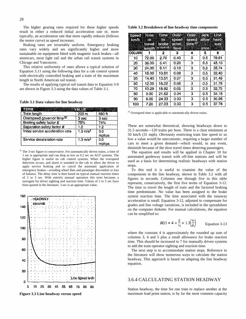
The results of applying typical rail transit data to Equation 3-9are shown in Figure 3.3 using the data values of Table 3.1.

Table 3.1 Data values for line headway

32 The 3-sec figure is conservative. For automatically driven trains, a time of1 sec is appropriate and can drop as low as 0.2 sec on AGT systems. Thehigher figure is useful on cab control systems. When the overspeeddetection occurs, and alarm is sounded in the cab to allow the driver toapply service braking and so cancel the automatic application ofemergency brakes—avoiding wheel flats and passenger discomfort or lossof balance. The delay time is then based on typical manual reaction timesof 2 to 3 sec. With entirely manual operation this term becomes asurrogate for driver sighting and reaction time. Values of 2 to 5 sec havebeen quoted in the literature. 3 sec is an appropriate value.

Figure 3.3 Line headway versus speed

Table 3.2 Breakdown of line headway time components

33 Overspeed time is applicable to automatically driven trains.

These are somewhat theoretical, showing headways down to31.5 seconds—120 trains per hour. There is a clear minimum at50 km/h (31 mph). Obviously restricting train line speed to solow a value would be uneconomic, requiring a larger number ofcars to meet a given demand—which would, in any event,diminish because of the slow travel times deterring passengers.

The equation and results will be applied in Chapter 10 forautomated guideway transit with off-line stations and will beused as a basis for determining realistic headways with stationstops.

To this end it is useful to examine the value of thecomponents in the line headway, shown in Table 3.2 with allfigures in seconds. Columns one through five in this tablerepresent, consecutively, the first five terms of Equation 3-12.The time to travel the length of train and the factored brakingtime predominate. No value has been assigned to the brakesystem reaction time. The time associated with the runawayacceleration is small. Equation 3-12, adjusted to compensate forgrades and line voltage variations, is included in the spreadsheeton the computer diskette. For manual calculations, the equationcan be simplified to:

Equation 3-13

where the constant 4 is approximately the rounded up sum ofcolumns 3, 4 and 5 plus a small allowance for brake reactiontime. This should be increased to 7 for manually driven systemsto add the train operator sighting and reaction time.

The next step is to accommodate station stops. Reference tothe literature will show numerous ways to calculate the stationheadway. This approach is based on adapting the line headwayequation.

3.6.4 CALCULATING STATION HEADWAY

Station headway, the time for one train to replace another at themaximum load point station, is by far the most common capacity

29

limitation. Having derived an expression for line headway thatuses readily available information with as few approximationsas possible, it is possible to adapt this to station headway by

• changing line speed to approach speed and solving for thisspeed,

• adding a component for the time a train takes to clear theplatform,

• adding the station dwell, and• adding an operating margin.

The time for a train to clear the platform is

Equation 3-14

Adding Equation 3-14 to 3-12 plus components for dwell and anoperating margin produces the station headway

Equation 3-15

where H(s) = station headway in secondsL = length of the longest train in metersD = distance from front of stopped train to start

of station exit block in metersva = station approach speed in m/svmax = maximum line speed in m/sK = braking safety factor—worst case service

braking is K% of specified normal rate—typically 75%

B = separation safety factor—equivalent tonumber of braking distances plus a margin,(surrogate for blocks) that separate trains

tos = time for overspeed governor to operatetjl = time lost to braking jerk limitation—

(seconds) typically 0.5 secondstbr = operator and brake system reaction timetd = dwell time (seconds)tom = operating margin (seconds)as = initial service acceleration rate in m/s2

ds = service deceleration rate in m/s2

Typical values will be used and this equation solved for theapproach speed under two circumstances:

1. three-aspect signaling system (B = 2.4)2. multiple command speed cab controls (B = 1.2)

A 45-sec dwell time is used—typical of the busiest stations onrail transit lines operating at capacity—together with anoperating margin time of 20 sec. The brake system reaction timewill use a moderate level of 1.5 sec—this should be higher forold air brake equipment, lower for modern electronic control,particularly with hydraulically actuated disk brakes. Otherfactors remain at the levels used in the line headway analysis.(See Table 3.3.) The results of solving Equation 3.15 for

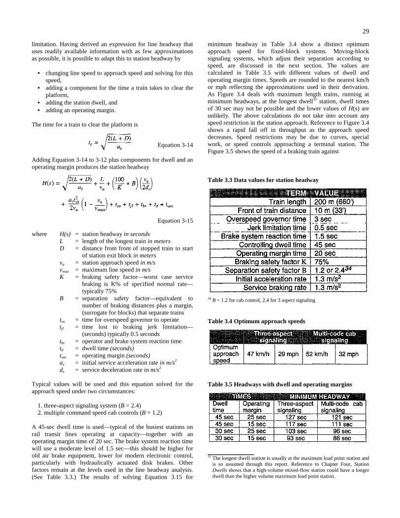
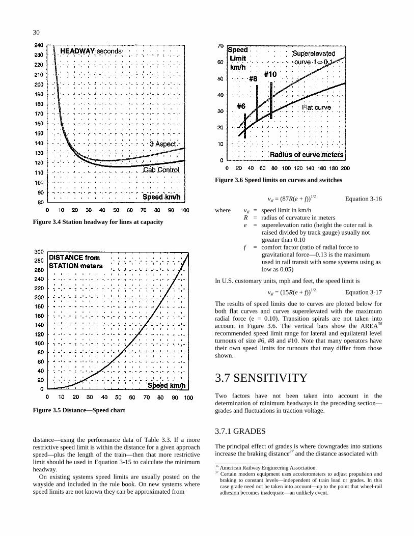
minimum headway in Table 3.4 show a distinct optimumapproach speed for fixed-block systems. Moving-blocksignaling systems, which adjust their separation according tospeed, are discussed in the next section. The values arecalculated in Table 3.5 with different values of dwell andoperating margin times. Speeds are rounded to the nearest km/hor mph reflecting the approximations used in their derivation.As Figure 3.4 deals with maximum length trains, running atminimum headways, at the longest dwell35 station, dwell timesof 30 sec may not be possible and the lower values of H(s) areunlikely. The above calculations do not take into account anyspeed restriction in the station approach. Reference to Figure 3.4shows a rapid fall off in throughput as the approach speeddecreases. Speed restrictions may be due to curves, specialwork, or speed controls approaching a terminal station. TheFigure 3.5 shows the speed of a braking train against

Table 3.3 Data values for station headway

34 B = 1.2 for cab control, 2.4 for 3 aspect signaling

Table 3.4 Optimum approach speeds

Table 3.5 Headways with dwell and operating margins

35 The longest dwell station is usually at the maximum load point station and

is so assumed through this report. Reference to Chapter Four, StationDwells shows that a high-volume mixed-flow station could have a longerdwell than the higher volume maximum load point station.

30

Figure 3.4 Station headway for lines at capacity

Figure 3.5 Distance—Speed chart

distance—using the performance data of Table 3.3. If a morerestrictive speed limit is within the distance for a given approachspeed—plus the length of the train—then that more restrictivelimit should be used in Equation 3-15 to calculate the minimumheadway.

On existing systems speed limits are usually posted on thewayside and included in the rule book. On new systems wherespeed limits are not known they can be approximated from

Figure 3.6 Speed limits on curves and switches

vsl = (87R(e + f))1/2 Equation 3-16

where vsl = speed limit in km/hR = radius of curvature in meterse = superelevation ratio (height the outer rail is

raised divided by track gauge) usually notgreater than 0.10

f = comfort factor (ratio of radial force togravitational force—0.13 is the maximumused in rail transit with some systems using aslow as 0.05)

In U.S. customary units, mph and feet, the speed limit is

vsl = (15R(e + f))1/2 Equation 3-17

The results of speed limits due to curves are plotted below forboth flat curves and curves superelevated with the maximumradial force (e = 0.10). Transition spirals are not taken intoaccount in Figure 3.6. The vertical bars show the AREA36

recommended speed limit range for lateral and equilateral levelturnouts of size #6, #8 and #10. Note that many operators havetheir own speed limits for turnouts that may differ from thoseshown.

3.7 SENSITIVITYTwo factors have not been taken into account in thedetermination of minimum headways in the preceding section—grades and fluctuations in traction voltage.

3.7.1 GRADES

The principal effect of grades is where downgrades into stationsincrease the braking distance37 and the distance associated with 36 American Railway Engineering Association.37 Certain modern equipment uses accelerometers to adjust propulsion and

braking to constant levels—independent of train load or grades. In thiscase grade need not be taken into account—up to the point that wheel-railadhesion becomes inadequate—an unlikely event.

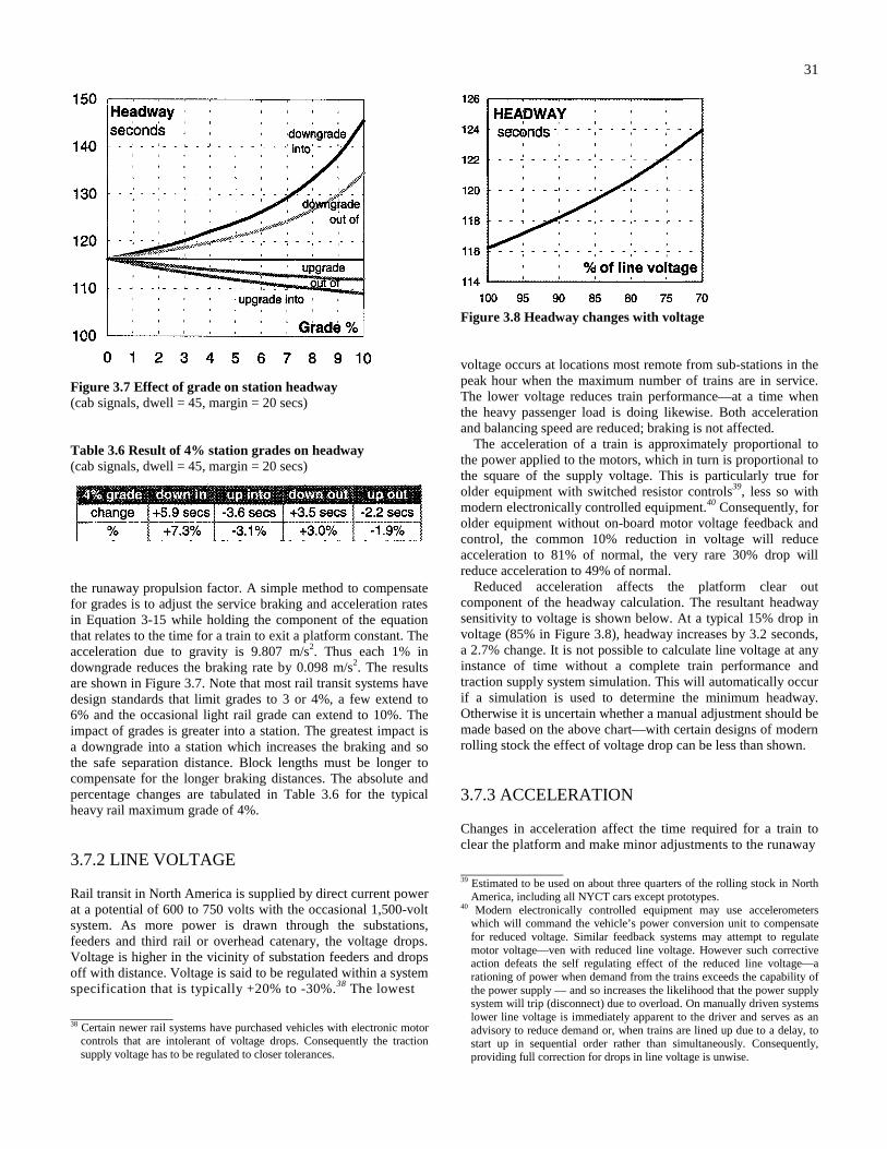
31

Figure 3.7 Effect of grade on station headway(cab signals, dwell = 45, margin = 20 secs)

Table 3.6 Result of 4% station grades on headway(cab signals, dwell = 45, margin = 20 secs)

the runaway propulsion factor. A simple method to compensatefor grades is to adjust the service braking and acceleration ratesin Equation 3-15 while holding the component of the equationthat relates to the time for a train to exit a platform constant. Theacceleration due to gravity is 9.807 m/s2. Thus each 1% indowngrade reduces the braking rate by 0.098 m/s2. The resultsare shown in Figure 3.7. Note that most rail transit systems havedesign standards that limit grades to 3 or 4%, a few extend to6% and the occasional light rail grade can extend to 10%. Theimpact of grades is greater into a station. The greatest impact isa downgrade into a station which increases the braking and sothe safe separation distance. Block lengths must be longer tocompensate for the longer braking distances. The absolute andpercentage changes are tabulated in Table 3.6 for the typicalheavy rail maximum grade of 4%.

3.7.2 LINE VOLTAGE

Rail transit in North America is supplied by direct current powerat a potential of 600 to 750 volts with the occasional 1,500-voltsystem. As more power is drawn through the substations,feeders and third rail or overhead catenary, the voltage drops.Voltage is higher in the vicinity of substation feeders and dropsoff with distance. Voltage is said to be regulated within a systemspecification that is typically +20% to -30%.38 The lowest

38 Certain newer rail systems have purchased vehicles with electronic motor

controls that are intolerant of voltage drops. Consequently the tractionsupply voltage has to be regulated to closer tolerances.

Figure 3.8 Headway changes with voltage

voltage occurs at locations most remote from sub-stations in thepeak hour when the maximum number of trains are in service.The lower voltage reduces train performance—at a time whenthe heavy passenger load is doing likewise. Both accelerationand balancing speed are reduced; braking is not affected.

The acceleration of a train is approximately proportional tothe power applied to the motors, which in turn is proportional tothe square of the supply voltage. This is particularly true forolder equipment with switched resistor controls39, less so withmodern electronically controlled equipment.40 Consequently, forolder equipment without on-board motor voltage feedback andcontrol, the common 10% reduction in voltage will reduceacceleration to 81% of normal, the very rare 30% drop willreduce acceleration to 49% of normal.

Reduced acceleration affects the platform clear outcomponent of the headway calculation. The resultant headwaysensitivity to voltage is shown below. At a typical 15% drop involtage (85% in Figure 3.8), headway increases by 3.2 seconds,a 2.7% change. It is not possible to calculate line voltage at anyinstance of time without a complete train performance andtraction supply system simulation. This will automatically occurif a simulation is used to determine the minimum headway.Otherwise it is uncertain whether a manual adjustment should bemade based on the above chart—with certain designs of modernrolling stock the effect of voltage drop can be less than shown.

3.7.3 ACCELERATION

Changes in acceleration affect the time required for a train toclear the platform and make minor adjustments to the runaway

39 Estimated to be used on about three quarters of the rolling stock in North

America, including all NYCT cars except prototypes.40 Modern electronically controlled equipment may use accelerometers

which will command the vehicle’s power conversion unit to compensatefor reduced voltage. Similar feedback systems may attempt to regulatemotor voltage—ven with reduced line voltage. However such correctiveaction defeats the self regulating effect of the reduced line voltage—arationing of power when demand from the trains exceeds the capability ofthe power supply — and so increases the likelihood that the power supplysystem will trip (disconnect) due to overload. On manually driven systemslower line voltage is immediately apparent to the driver and serves as anadvisory to reduce demand or, when trains are lined up due to a delay, tostart up in sequential order rather than simultaneously. Consequently,providing full correction for drops in line voltage is unwise.

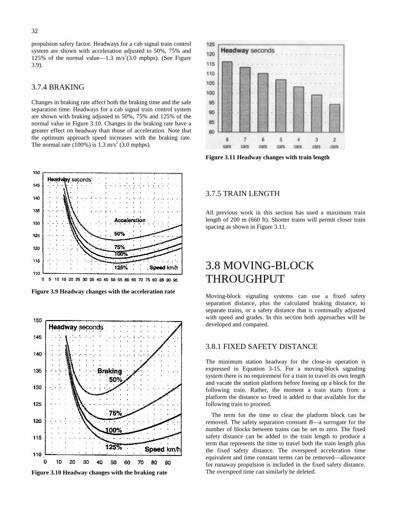
32

propulsion safety factor. Headways for a cab signal train controlsystem are shown with acceleration adjusted to 50%, 75% and125% of the normal value—1.3 m/s2(3.0 mphps). (See Figure3.9).

3.7.4 BRAKING

Changes in braking rate affect both the braking time and the safeseparation time. Headways for a cab signal train control systemare shown with braking adjusted to 50%, 75% and 125% of thenormal value in Figure 3.10. Changes in the braking rate have agreater effect on headway than those of acceleration. Note thatthe optimum approach speed increases with the braking rate.The normal rate (100%) is 1.3 m/s2 (3.0 mphps).

Figure 3.9 Headway changes with the acceleration rate

Figure 3.10 Headway changes with the braking rate

Figure 3.11 Headway changes with train length

3.7.5 TRAIN LENGTH

All previous work in this section has used a maximum trainlength of 200 m (660 ft). Shorter trains will permit closer trainspacing as shown in Figure 3.11.

3.8 MOVING-BLOCKTHROUGHPUTMoving-block signaling systems can use a fixed safetyseparation distance, plus the calculated braking distance, toseparate trains, or a safety distance that is continually adjustedwith speed and grades. In this section both approaches will bedeveloped and compared.

3.8.1 FIXED SAFETY DISTANCE

The minimum station headway for the close-in operation isexpressed in Equation 3-15. For a moving-block signalingsystem there is no requirement for a train to travel its own lengthand vacate the station platform before freeing up a block for thefollowing train. Rather, the moment a train starts from aplatform the distance so freed is added to that available for thefollowing train to proceed.

The term for the time to clear the platform block can beremoved. The safety separation constant B—a surrogate for thenumber of blocks between trains can be set to zero. The fixedsafety distance can be added to the train length to produce aterm that represents the time to travel both the train length plusthe fixed safety distance. The overspeed acceleration timeequivalent and time constant terms can be removed—allowancefor runaway propulsion is included in the fixed safety distance.The overspeed time can similarly be deleted.

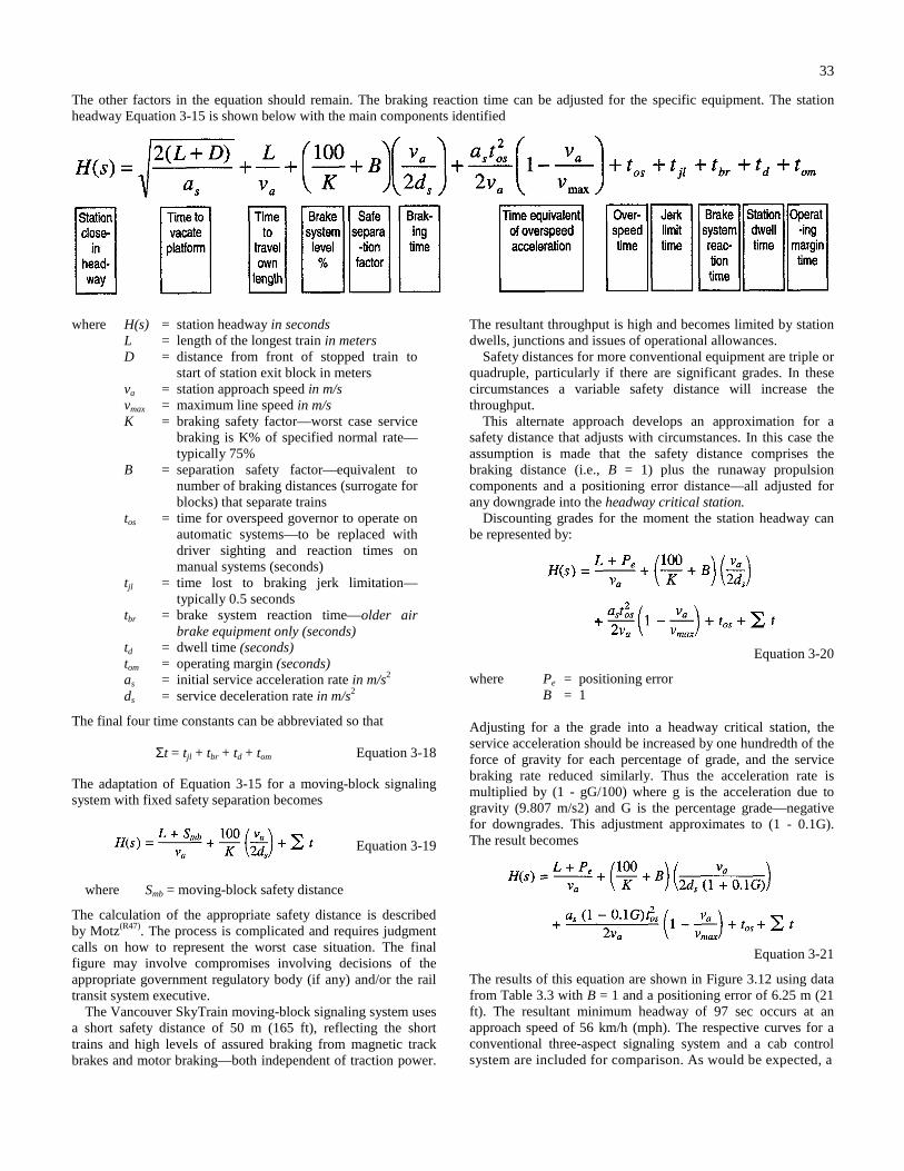
33

The other factors in the equation should remain. The braking reaction time can be adjusted for the specific equipment. The stationheadway Equation 3-15 is shown below with the main components identified

where H(s) = station headway in secondsL = length of the longest train in metersD = distance from front of stopped train to

start of station exit block in metersva = station approach speed in m/svmax = maximum line speed in m/sK = braking safety factor—worst case service

braking is K% of specified normal rate—typically 75%

B = separation safety factor—equivalent tonumber of braking distances (surrogate forblocks) that separate trains

tos = time for overspeed governor to operate onautomatic systems—to be replaced withdriver sighting and reaction times onmanual systems (seconds)

tjl = time lost to braking jerk limitation—typically 0.5 seconds

tbr = brake system reaction time—older airbrake equipment only (seconds)

td = dwell time (seconds)tom = operating margin (seconds)as = initial service acceleration rate in m/s2

ds = service deceleration rate in m/s2

The final four time constants can be abbreviated so that

Σt = tjl + tbr + td + tom Equation 3-18

The adaptation of Equation 3-15 for a moving-block signalingsystem with fixed safety separation becomes

Equation 3-19

where Smb = moving-block safety distance

The calculation of the appropriate safety distance is describedby Motz(R47). The process is complicated and requires judgmentcalls on how to represent the worst case situation. The finalfigure may involve compromises involving decisions of theappropriate government regulatory body (if any) and/or the railtransit system executive.

The Vancouver SkyTrain moving-block signaling system usesa short safety distance of 50 m (165 ft), reflecting the shorttrains and high levels of assured braking from magnetic trackbrakes and motor braking—both independent of traction power.

The resultant throughput is high and becomes limited by stationdwells, junctions and issues of operational allowances.

Safety distances for more conventional equipment are triple orquadruple, particularly if there are significant grades. In thesecircumstances a variable safety distance will increase thethroughput.

This alternate approach develops an approximation for asafety distance that adjusts with circumstances. In this case theassumption is made that the safety distance comprises thebraking distance (i.e., B = 1) plus the runaway propulsioncomponents and a positioning error distance—all adjusted forany downgrade into the headway critical station.

Discounting grades for the moment the station headway canbe represented by:

Equation 3-20

where Pe = positioning errorB = 1

Adjusting for a the grade into a headway critical station, theservice acceleration should be increased by one hundredth of theforce of gravity for each percentage of grade, and the servicebraking rate reduced similarly. Thus the acceleration rate ismultiplied by (1 - gG/100) where g is the acceleration due togravity (9.807 m/s2) and G is the percentage grade—negativefor downgrades. This adjustment approximates to (1 - 0.1G).The result becomes

Equation 3-21

The results of this equation are shown in Figure 3.12 using datafrom Table 3.3 with B = 1 and a positioning error of 6.25 m (21ft). The resultant minimum headway of 97 sec occurs at anapproach speed of 56 km/h (mph). The respective curves for aconventional three-aspect signaling system and a cab controlsystem are included for comparison. As would be expected, a

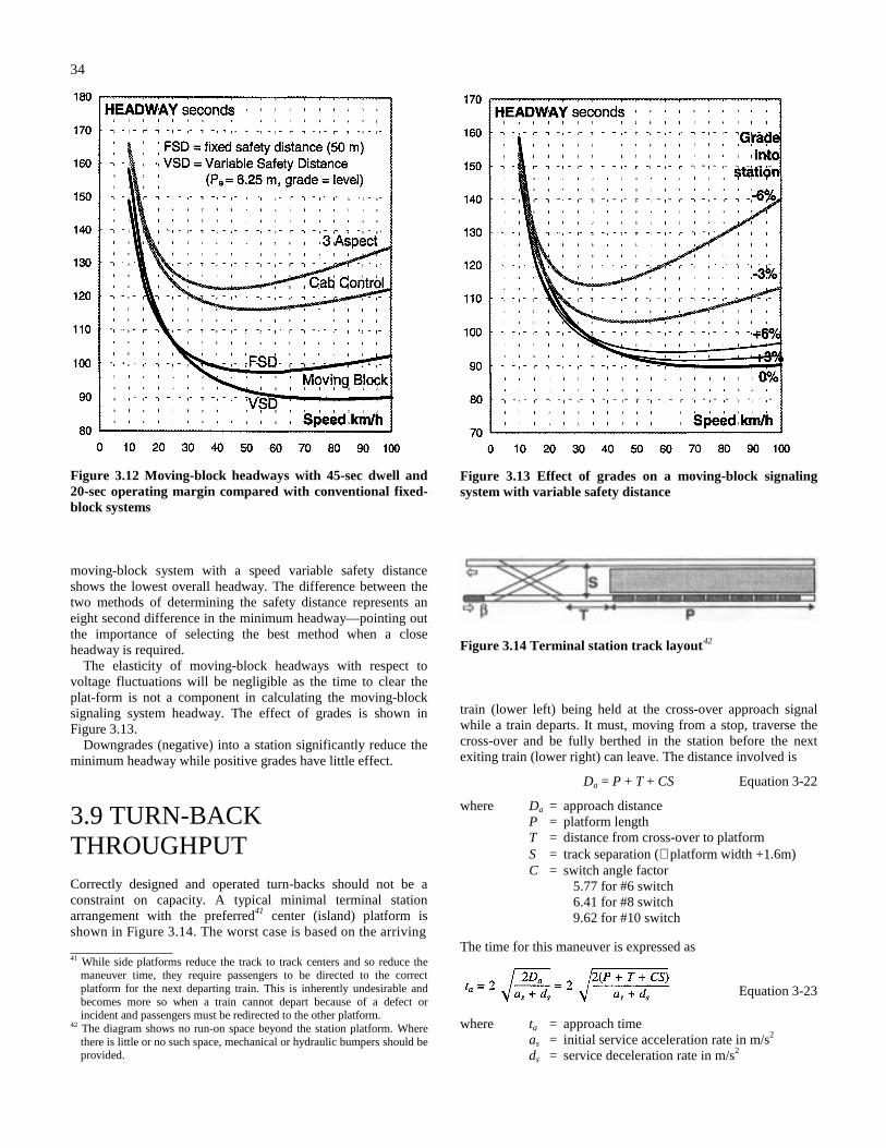
34

Figure 3.12 Moving-block headways with 45-sec dwell and20-sec operating margin compared with conventional fixed-block systems

moving-block system with a speed variable safety distanceshows the lowest overall headway. The difference between thetwo methods of determining the safety distance represents aneight second difference in the minimum headway—pointing outthe importance of selecting the best method when a closeheadway is required.

The elasticity of moving-block headways with respect tovoltage fluctuations will be negligible as the time to clear theplat-form is not a component in calculating the moving-blocksignaling system headway. The effect of grades is shown inFigure 3.13.

Downgrades (negative) into a station significantly reduce theminimum headway while positive grades have little effect.

3.9 TURN-BACKTHROUGHPUTCorrectly designed and operated turn-backs should not be aconstraint on capacity. A typical minimal terminal stationarrangement with the preferred41 center (island) platform isshown in Figure 3.14. The worst case is based on the arriving 41 While side platforms reduce the track to track centers and so reduce the

maneuver time, they require passengers to be directed to the correctplatform for the next departing train. This is inherently undesirable andbecomes more so when a train cannot depart because of a defect orincident and passengers must be redirected to the other platform.

42 The diagram shows no run-on space beyond the station platform. Wherethere is little or no such space, mechanical or hydraulic bumpers should beprovided.

Figure 3.13 Effect of grades on a moving-block signalingsystem with variable safety distance

Figure 3.14 Terminal station track layout42

train (lower left) being held at the cross-over approach signalwhile a train departs. It must, moving from a stop, traverse thecross-over and be fully berthed in the station before the nextexiting train (lower right) can leave. The distance involved is

Da = P + T + CS Equation 3-22

where Da = approach distanceP = platform lengthT = distance from cross-over to platformS = track separation (≅ platform width +1.6m)C = switch angle factor

5.77 for #6 switch6.41 for #8 switch9.62 for #10 switch

The time for this maneuver is expressed as

Equation 3-23

where ta = approach timeas = initial service acceleration rate in m/s2

ds = service deceleration rate in m/s2

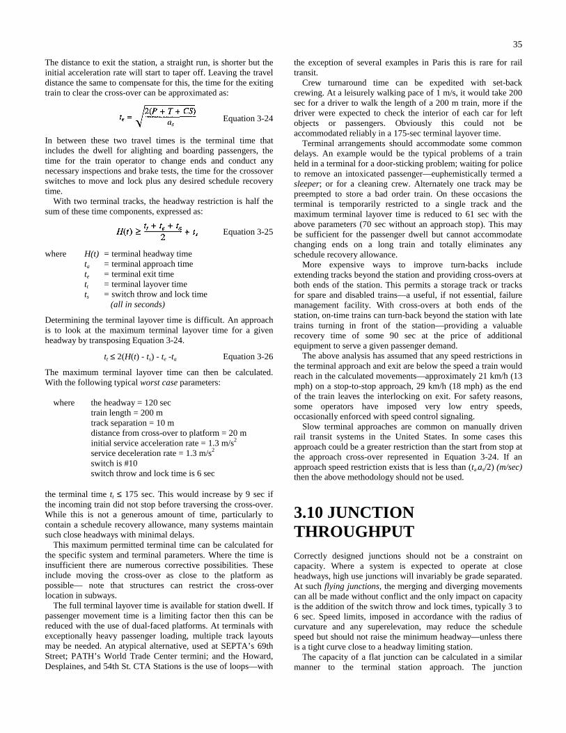
35

The distance to exit the station, a straight run, is shorter but theinitial acceleration rate will start to taper off. Leaving the traveldistance the same to compensate for this, the time for the exitingtrain to clear the cross-over can be approximated as:

Equation 3-24

In between these two travel times is the terminal time thatincludes the dwell for alighting and boarding passengers, thetime for the train operator to change ends and conduct anynecessary inspections and brake tests, the time for the crossoverswitches to move and lock plus any desired schedule recoverytime.

With two terminal tracks, the headway restriction is half thesum of these time components, expressed as:

Equation 3-25

where H(t) = terminal headway timeta = terminal approach timete = terminal exit timett = terminal layover timets = switch throw and lock time

(all in seconds)

Determining the terminal layover time is difficult. An approachis to look at the maximum terminal layover time for a givenheadway by transposing Equation 3-24.

tt ≤ 2(H(t) - ts) - te -ta Equation 3-26

The maximum terminal layover time can then be calculated.With the following typical worst case parameters:

where the headway = 120 sectrain length = 200 mtrack separation = 10 mdistance from cross-over to platform = 20 minitial service acceleration rate = 1.3 m/s2

service deceleration rate = 1.3 m/s2

switch is #10switch throw and lock time is 6 sec

the terminal time tt ≤ 175 sec. This would increase by 9 sec ifthe incoming train did not stop before traversing the cross-over.While this is not a generous amount of time, particularly tocontain a schedule recovery allowance, many systems maintainsuch close headways with minimal delays.

This maximum permitted terminal time can be calculated forthe specific system and terminal parameters. Where the time isinsufficient there are numerous corrective possibilities. Theseinclude moving the cross-over as close to the platform aspossible— note that structures can restrict the cross-overlocation in subways.

The full terminal layover time is available for station dwell. Ifpassenger movement time is a limiting factor then this can bereduced with the use of dual-faced platforms. At terminals withexceptionally heavy passenger loading, multiple track layoutsmay be needed. An atypical alternative, used at SEPTA’s 69thStreet; PATH’s World Trade Center termini; and the Howard,Desplaines, and 54th St. CTA Stations is the use of loops—with

the exception of several examples in Paris this is rare for railtransit.

Crew turnaround time can be expedited with set-backcrewing. At a leisurely walking pace of 1 m/s, it would take 200sec for a driver to walk the length of a 200 m train, more if thedriver were expected to check the interior of each car for leftobjects or passengers. Obviously this could not beaccommodated reliably in a 175-sec terminal layover time.

Terminal arrangements should accommodate some commondelays. An example would be the typical problems of a trainheld in a terminal for a door-sticking problem; waiting for policeto remove an intoxicated passenger—euphemistically termed asleeper; or for a cleaning crew. Alternately one track may bepreempted to store a bad order train. On these occasions theterminal is temporarily restricted to a single track and themaximum terminal layover time is reduced to 61 sec with theabove parameters (70 sec without an approach stop). This maybe sufficient for the passenger dwell but cannot accommodatechanging ends on a long train and totally eliminates anyschedule recovery allowance.

More expensive ways to improve turn-backs includeextending tracks beyond the station and providing cross-overs atboth ends of the station. This permits a storage track or tracksfor spare and disabled trains—a useful, if not essential, failuremanagement facility. With cross-overs at both ends of thestation, on-time trains can turn-back beyond the station with latetrains turning in front of the station—providing a valuablerecovery time of some 90 sec at the price of additionalequipment to serve a given passenger demand.

The above analysis has assumed that any speed restrictions inthe terminal approach and exit are below the speed a train wouldreach in the calculated movements—approximately 21 km/h (13mph) on a stop-to-stop approach, 29 km/h (18 mph) as the endof the train leaves the interlocking on exit. For safety reasons,some operators have imposed very low entry speeds,occasionally enforced with speed control signaling.

Slow terminal approaches are common on manually drivenrail transit systems in the United States. In some cases thisapproach could be a greater restriction than the start from stop atthe approach cross-over represented in Equation 3-24. If anapproach speed restriction exists that is less than (ta·as/2) (m/sec)then the above methodology should not be used.

3.10 JUNCTIONTHROUGHPUTCorrectly designed junctions should not be a constraint oncapacity. Where a system is expected to operate at closeheadways, high use junctions will invariably be grade separated.At such flying junctions, the merging and diverging movementscan all be made without conflict and the only impact on capacityis the addition of the switch throw and lock times, typically 3 to6 sec. Speed limits, imposed in accordance with the radius ofcurvature and any superelevation, may reduce the schedulespeed but should not raise the minimum headway—unless thereis a tight curve close to a headway limiting station.

The capacity of a flat junction can be calculated in a similarmanner to the terminal station approach. The junction

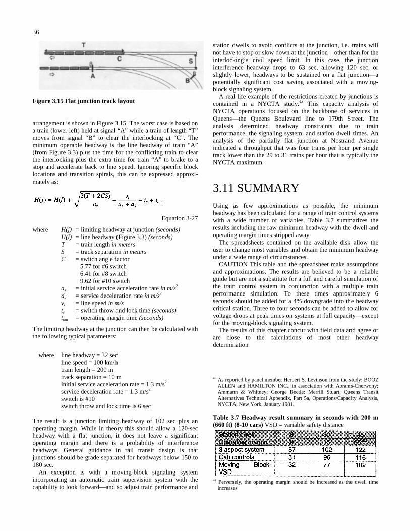
36

Figure 3.15 Flat junction track layout

arrangement is shown in Figure 3.15. The worst case is based ona train (lower left) held at signal “A” while a train of length “T”moves from signal “B” to clear the interlocking at “C”. Theminimum operable headway is the line headway of train “A”(from Figure 3.3) plus the time for the conflicting train to clearthe interlocking plus the extra time for train “A” to brake to astop and accelerate back to line speed. Ignoring specific blocklocations and transition spirals, this can be expressed approxi-mately as:

Equation 3-27

where H(j) = limiting headway at junction (seconds)H(l) = line headway (Figure 3.3) (seconds)T = train length in metersS = track separation in metersC = switch angle factor

5.77 for #6 switch6.41 for #8 switch9.62 for #10 switch

as = initial service acceleration rate in m/s2

ds = service deceleration rate in m/s2

vl = line speed in m/sts = switch throw and lock time (seconds)tom = operating margin time (seconds)

The limiting headway at the junction can then be calculated withthe following typical parameters:

where line headway = 32 secline speed = 100 km/htrain length = 200 mtrack separation = 10 minitial service acceleration rate = 1.3 m/s2

service deceleration rate = 1.3 m/s2

switch is #10switch throw and lock time is 6 sec

The result is a junction limiting headway of 102 sec plus anoperating margin. While in theory this should allow a 120-secheadway with a flat junction, it does not leave a significantoperating margin and there is a probability of interferenceheadways. General guidance in rail transit design is thatjunctions should be grade separated for headways below 150 to180 sec.

An exception is with a moving-block signaling systemincorporating an automatic train supervision system with thecapability to look forward—and so adjust train performance and

station dwells to avoid conflicts at the junction, i.e. trains willnot have to stop or slow down at the junction—other than for theinterlocking’s civil speed limit. In this case, the junctioninterference headway drops to 63 sec, allowing 120 sec, orslightly lower, headways to be sustained on a flat junction—apotentially significant cost saving associated with a moving-block signaling system.

A real-life example of the restrictions created by junctions iscontained in a NYCTA study.43 This capacity analysis ofNYCTA operations focused on the backbone of services inQueens—the Queens Boulevard line to 179th Street. Theanalysis determined headway constraints due to trainperformance, the signaling system, and station dwell times. Ananalysis of the partially flat junction at Nostrand Avenueindicated a throughput that was four trains per hour per singletrack lower than the 29 to 31 trains per hour that is typically theNYCTA maximum.

3.11 SUMMARYUsing as few approximations as possible, the minimumheadway has been calculated for a range of train control systemswith a wide number of variables. Table 3.7 summarizes theresults including the raw minimum headway with the dwell andoperating margin times stripped away.

The spreadsheets contained on the available disk allow theuser to change most variables and obtain the minimum headwayunder a wide range of circumstances.

CAUTION This table and the spreadsheet make assumptionsand approximations. The results are believed to be a reliableguide but are not a substitute for a full and careful simulation ofthe train control system in conjunction with a multiple trainperformance simulation. To these times approximately 6seconds should be added for a 4% downgrade into the headwaycritical station. Three to four seconds can be added to allow forvoltage drops at peak times on systems at full capacity—exceptfor the moving-block signaling system.

The results of this chapter concur with field data and agree orare close to the calculations of most other headwaydetermination

43 As reported by panel member Herbert S. Levinson from the study: BOOZ

ALLEN and HAMILTON INC., in association with Abrams-Cherwony;Ammann & Whitney; George Beetle: Merrill Stuart, Queens TransitAlternatives Technical Appendix, Part 5a, Operations/Capacity Analysis,NYCTA, New York, January 1981.

Table 3.7 Headway result summary in seconds with 200 m(660 ft) (8-10 cars) VSD = variable safety distance

44 Perversely, the operating margin should be increased as the dwell timeincreases

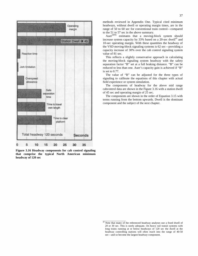
37

Figure 3.16 Headway components for cab control signalingthat comprise the typical North American minimumheadway of 120 sec

methods reviewed in Appendix One. Typical cited minimumheadways, without dwell or operating margin times, are in therange of 50 to 60 sec for conventional train control—comparedto the 51 to 57 sec in the above summary.

Auer(R09) estimates that a moving-block system shouldincrease system capacity by 33% based on a 20-sec dwell45 and10-sec operating margin. With these quantities the headway ofthe VSD moving-block signaling systems is 62 sec—providing acapacity increase of 30% over the cab control signaling systemvalue of 81 sec.

This reflects a slightly conservative approach in calculatingthe moving-block signaling system headway with the safetyseparation factor “B” set at a full braking distance. “B” can bereduced to less than one. Auer’s capacity gain is achieved if “B”is set to 0.77.

The value of “B” can be adjusted for the three types ofsignaling to calibrate the equations of this chapter with actualfield experience or system simulation.

The components of headway for the above mid rangecabcontrol data are shown in the Figure 3.16 with a station dwellof 45 sec and operating margin of 25 sec.

The components are shown in the order of Equation 3.15 withterms running from the bottom upwards. Dwell is the dominantcomponent and the subject of the next chapter.

45 Note that many of the referenced headway analyses use a fixed dwell of

20 or 30 sec. This is rarely adequate. On heavy rail transit systems withlong trains running at or below headways of 120 sec the dwell at theheadway controlling stations will often reach into the range of 40-50sec—and so become the largest headway component.

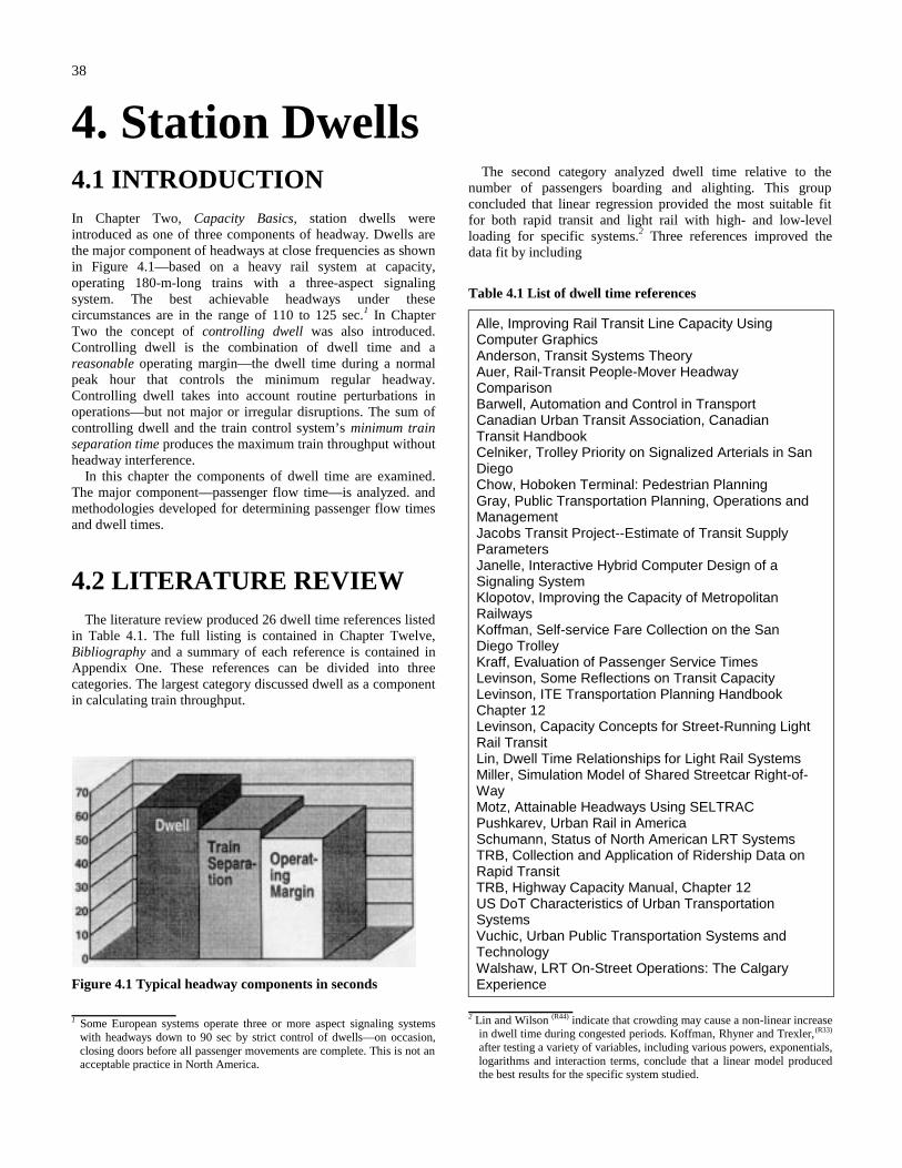
38

4. Station Dwells4.1 INTRODUCTIONIn Chapter Two, Capacity Basics, station dwells wereintroduced as one of three components of headway. Dwells arethe major component of headways at close frequencies as shownin Figure 4.1—based on a heavy rail system at capacity,operating 180-m-long trains with a three-aspect signalingsystem. The best achievable headways under thesecircumstances are in the range of 110 to 125 sec.1 In ChapterTwo the concept of controlling dwell was also introduced.Controlling dwell is the combination of dwell time and areasonable operating margin—the dwell time during a normalpeak hour that controls the minimum regular headway.Controlling dwell takes into account routine perturbations inoperations—but not major or irregular disruptions. The sum ofcontrolling dwell and the train control system’s minimum trainseparation time produces the maximum train throughput withoutheadway interference.

In this chapter the components of dwell time are examined.The major component—passenger flow time—is analyzed. andmethodologies developed for determining passenger flow timesand dwell times.

4.2 LITERATURE REVIEWThe literature review produced 26 dwell time references listed

in Table 4.1. The full listing is contained in Chapter Twelve,Bibliography and a summary of each reference is contained inAppendix One. These references can be divided into threecategories. The largest category discussed dwell as a componentin calculating train throughput.

Figure 4.1 Typical headway components in seconds

1 Some European systems operate three or more aspect signaling systems

with headways down to 90 sec by strict control of dwells—on occasion,closing doors before all passenger movements are complete. This is not anacceptable practice in North America.

The second category analyzed dwell time relative to thenumber of passengers boarding and alighting. This groupconcluded that linear regression provided the most suitable fitfor both rapid transit and light rail with high- and low-levelloading for specific systems.2 Three references improved thedata fit by including

Table 4.1 List of dwell time references

Alle, Improving Rail Transit Line Capacity UsingComputer GraphicsAnderson, Transit Systems TheoryAuer, Rail-Transit People-Mover HeadwayComparisonBarwell, Automation and Control in TransportCanadian Urban Transit Association, CanadianTransit HandbookCelniker, Trolley Priority on Signalized Arterials in SanDiegoChow, Hoboken Terminal: Pedestrian PlanningGray, Public Transportation Planning, Operations andManagementJacobs Transit Project--Estimate of Transit SupplyParametersJanelle, Interactive Hybrid Computer Design of aSignaling SystemKlopotov, Improving the Capacity of MetropolitanRailwaysKoffman, Self-service Fare Collection on the SanDiego TrolleyKraff, Evaluation of Passenger Service TimesLevinson, Some Reflections on Transit CapacityLevinson, ITE Transportation Planning HandbookChapter 12Levinson, Capacity Concepts for Street-Running LightRail TransitLin, Dwell Time Relationships for Light Rail SystemsMiller, Simulation Model of Shared Streetcar Right-of-WayMotz, Attainable Headways Using SELTRACPushkarev, Urban Rail in AmericaSchumann, Status of North American LRT SystemsTRB, Collection and Application of Ridership Data onRapid TransitTRB, Highway Capacity Manual, Chapter 12US DoT Characteristics of Urban TransportationSystemsVuchic, Urban Public Transportation Systems andTechnologyWalshaw, LRT On-Street Operations: The CalgaryExperience

2 Lin and Wilson (R44) indicate that crowding may cause a non-linear increase

in dwell time during congested periods. Koffman, Rhyner and Trexler,(R33)

after testing a variety of variables, including various powers, exponentials,logarithms and interaction terms, conclude that a linear model producedthe best results for the specific system studied.

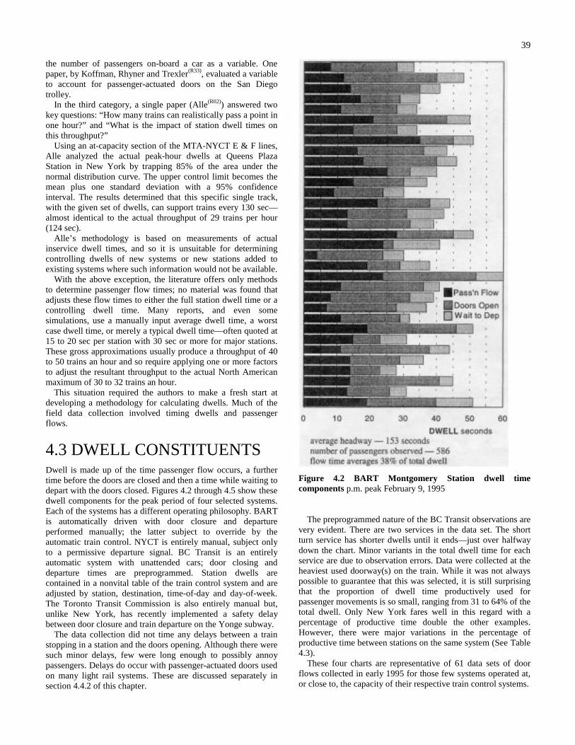
39

the number of passengers on-board a car as a variable. Onepaper, by Koffman, Rhyner and Trexler(R33), evaluated a variableto account for passenger-actuated doors on the San Diegotrolley.

In the third category, a single paper (Alle(R02)) answered twokey questions: “How many trains can realistically pass a point inone hour?” and “What is the impact of station dwell times onthis throughput?”

Using an at-capacity section of the MTA-NYCT E & F lines,Alle analyzed the actual peak-hour dwells at Queens PlazaStation in New York by trapping 85% of the area under thenormal distribution curve. The upper control limit becomes themean plus one standard deviation with a 95% confidenceinterval. The results determined that this specific single track,with the given set of dwells, can support trains every 130 sec—almost identical to the actual throughput of 29 trains per hour(124 sec).

Alle’s methodology is based on measurements of actualinservice dwell times, and so it is unsuitable for determiningcontrolling dwells of new systems or new stations added toexisting systems where such information would not be available.

With the above exception, the literature offers only methodsto determine passenger flow times; no material was found thatadjusts these flow times to either the full station dwell time or acontrolling dwell time. Many reports, and even somesimulations, use a manually input average dwell time, a worstcase dwell time, or merely a typical dwell time—often quoted at15 to 20 sec per station with 30 sec or more for major stations.These gross approximations usually produce a throughput of 40to 50 trains an hour and so require applying one or more factorsto adjust the resultant throughput to the actual North Americanmaximum of 30 to 32 trains an hour.

This situation required the authors to make a fresh start atdeveloping a methodology for calculating dwells. Much of thefield data collection involved timing dwells and passengerflows.

4.3 DWELL CONSTITUENTSDwell is made up of the time passenger flow occurs, a furthertime before the doors are closed and then a time while waiting todepart with the doors closed. Figures 4.2 through 4.5 show thesedwell components for the peak period of four selected systems.Each of the systems has a different operating philosophy. BARTis automatically driven with door closure and departureperformed manually; the latter subject to override by theautomatic train control. NYCT is entirely manual, subject onlyto a permissive departure signal. BC Transit is an entirelyautomatic system with unattended cars; door closing anddeparture times are preprogrammed. Station dwells arecontained in a nonvital table of the train control system and areadjusted by station, destination, time-of-day and day-of-week.The Toronto Transit Commission is also entirely manual but,unlike New York, has recently implemented a safety delaybetween door closure and train departure on the Yonge subway.

The data collection did not time any delays between a trainstopping in a station and the doors opening. Although there weresuch minor delays, few were long enough to possibly annoypassengers. Delays do occur with passenger-actuated doors usedon many light rail systems. These are discussed separately insection 4.4.2 of this chapter.

Figure 4.2 BART Montgomery Station dwell timecomponents p.m. peak February 9, 1995

The preprogrammed nature of the BC Transit observations arevery evident. There are two services in the data set. The shortturn service has shorter dwells until it ends—just over halfwaydown the chart. Minor variants in the total dwell time for eachservice are due to observation errors. Data were collected at theheaviest used doorway(s) on the train. While it was not alwayspossible to guarantee that this was selected, it is still surprisingthat the proportion of dwell time productively used forpassenger movements is so small, ranging from 31 to 64% of thetotal dwell. Only New York fares well in this regard with apercentage of productive time double the other examples.However, there were major variations in the percentage ofproductive time between stations on the same system (See Table4.3).

These four charts are representative of 61 data sets of doorflows collected in early 1995 for those few systems operated at,or close to, the capacity of their respective train control systems.

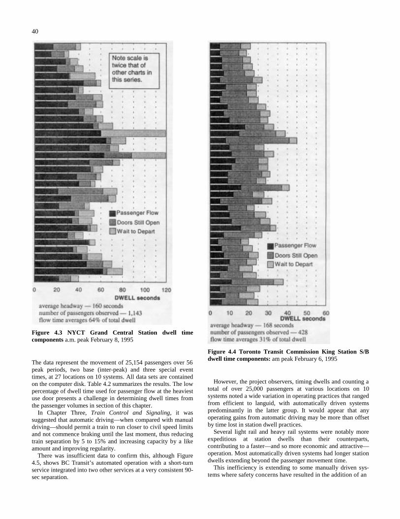
40

Figure 4.3 NYCT Grand Central Station dwell timecomponents a.m. peak February 8, 1995

The data represent the movement of 25,154 passengers over 56peak periods, two base (inter-peak) and three special eventtimes, at 27 locations on 10 systems. All data sets are containedon the computer disk. Table 4.2 summarizes the results. The lowpercentage of dwell time used for passenger flow at the heaviestuse door presents a challenge in determining dwell times fromthe passenger volumes in section of this chapter.

In Chapter Three, Train Control and Signaling, it wassuggested that automatic driving—when compared with manualdriving—should permit a train to run closer to civil speed limitsand not commence braking until the last moment, thus reducingtrain separation by 5 to 15% and increasing capacity by a likeamount and improving regularity.

There was insufficient data to confirm this, although Figure4.5, shows BC Transit’s automated operation with a short-turnservice integrated into two other services at a very consistent 90-sec separation.

Figure 4.4 Toronto Transit Commission King Station S/Bdwell time components: am peak February 6, 1995

However, the project observers, timing dwells and counting atotal of over 25,000 passengers at various locations on 10systems noted a wide variation in operating practices that rangedfrom efficient to languid, with automatically driven systemspredominantly in the latter group. It would appear that anyoperating gains from automatic driving may be more than offsetby time lost in station dwell practices.

Several light rail and heavy rail systems were notably moreexpeditious at station dwells than their counterparts,contributing to a faster—and so more economic and attractive—operation. Most automatically driven systems had longer stationdwells extending beyond the passenger movement time.

This inefficiency is extending to some manually driven sys-tems where safety concerns have resulted in the addition of an

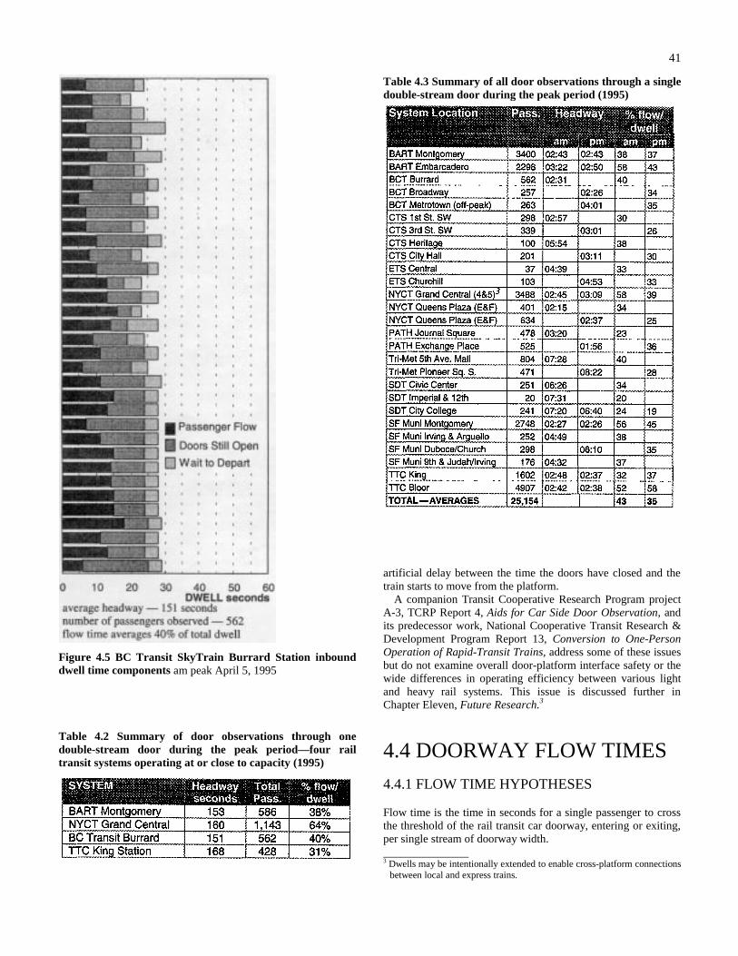
41

Figure 4.5 BC Transit SkyTrain Burrard Station inbounddwell time components am peak April 5, 1995

Table 4.2 Summary of door observations through onedouble-stream door during the peak period—four railtransit systems operating at or close to capacity (1995)

Table 4.3 Summary of all door observations through a singledouble-stream door during the peak period (1995)

artificial delay between the time the doors have closed and thetrain starts to move from the platform.

A companion Transit Cooperative Research Program projectA-3, TCRP Report 4, Aids for Car Side Door Observation, andits predecessor work, National Cooperative Transit Research &Development Program Report 13, Conversion to One-PersonOperation of Rapid-Transit Trains, address some of these issuesbut do not examine overall door-platform interface safety or thewide differences in operating efficiency between various lightand heavy rail systems. This issue is discussed further inChapter Eleven, Future Research.3

4.4 DOORWAY FLOW TIMES

4.4.1 FLOW TIME HYPOTHESES

Flow time is the time in seconds for a single passenger to crossthe threshold of the rail transit car doorway, entering or exiting,per single stream of doorway width. 3 Dwells may be intentionally extended to enable cross-platform connections

between local and express trains.

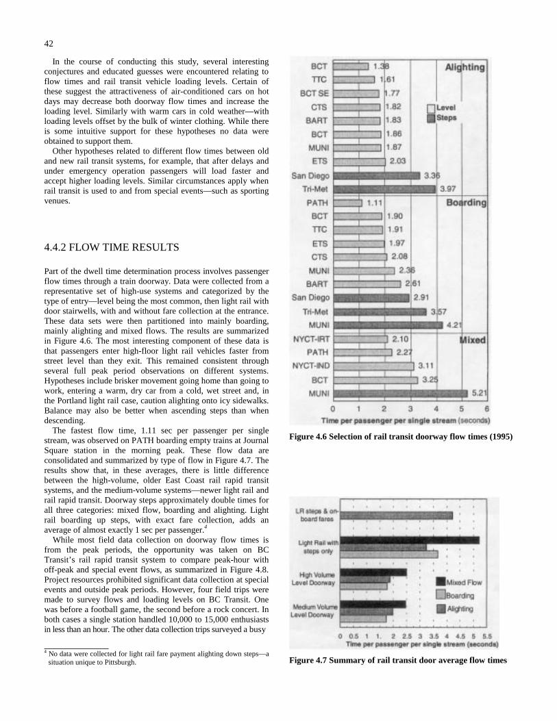
42

In the course of conducting this study, several interestingconjectures and educated guesses were encountered relating toflow times and rail transit vehicle loading levels. Certain ofthese suggest the attractiveness of air-conditioned cars on hotdays may decrease both doorway flow times and increase theloading level. Similarly with warm cars in cold weather—withloading levels offset by the bulk of winter clothing. While thereis some intuitive support for these hypotheses no data wereobtained to support them.

Other hypotheses related to different flow times between oldand new rail transit systems, for example, that after delays andunder emergency operation passengers will load faster andaccept higher loading levels. Similar circumstances apply whenrail transit is used to and from special events—such as sportingvenues.

4.4.2 FLOW TIME RESULTS

Part of the dwell time determination process involves passengerflow times through a train doorway. Data were collected from arepresentative set of high-use systems and categorized by thetype of entry—level being the most common, then light rail withdoor stairwells, with and without fare collection at the entrance.These data sets were then partitioned into mainly boarding,mainly alighting and mixed flows. The results are summarizedin Figure 4.6. The most interesting component of these data isthat passengers enter high-floor light rail vehicles faster fromstreet level than they exit. This remained consistent throughseveral full peak period observations on different systems.Hypotheses include brisker movement going home than going towork, entering a warm, dry car from a cold, wet street and, inthe Portland light rail case, caution alighting onto icy sidewalks.Balance may also be better when ascending steps than whendescending.

The fastest flow time, 1.11 sec per passenger per singlestream, was observed on PATH boarding empty trains at JournalSquare station in the morning peak. These flow data areconsolidated and summarized by type of flow in Figure 4.7. Theresults show that, in these averages, there is little differencebetween the high-volume, older East Coast rail rapid transitsystems, and the medium-volume systems—newer light rail andrail rapid transit. Doorway steps approximately double times forall three categories: mixed flow, boarding and alighting. Lightrail boarding up steps, with exact fare collection, adds anaverage of almost exactly 1 sec per passenger.4

While most field data collection on doorway flow times isfrom the peak periods, the opportunity was taken on BCTransit’s rail rapid transit system to compare peak-hour withoff-peak and special event flows, as summarized in Figure 4.8.Project resources prohibited significant data collection at specialevents and outside peak periods. However, four field trips weremade to survey flows and loading levels on BC Transit. Onewas before a football game, the second before a rock concert. Inboth cases a single station handled 10,000 to 15,000 enthusiastsin less than an hour. The other data collection trips surveyed a busy

4 No data were collected for light rail fare payment alighting down steps—a

situation unique to Pittsburgh.

Figure 4.6 Selection of rail transit doorway flow times (1995)

Figure 4.7 Summary of rail transit door average flow times

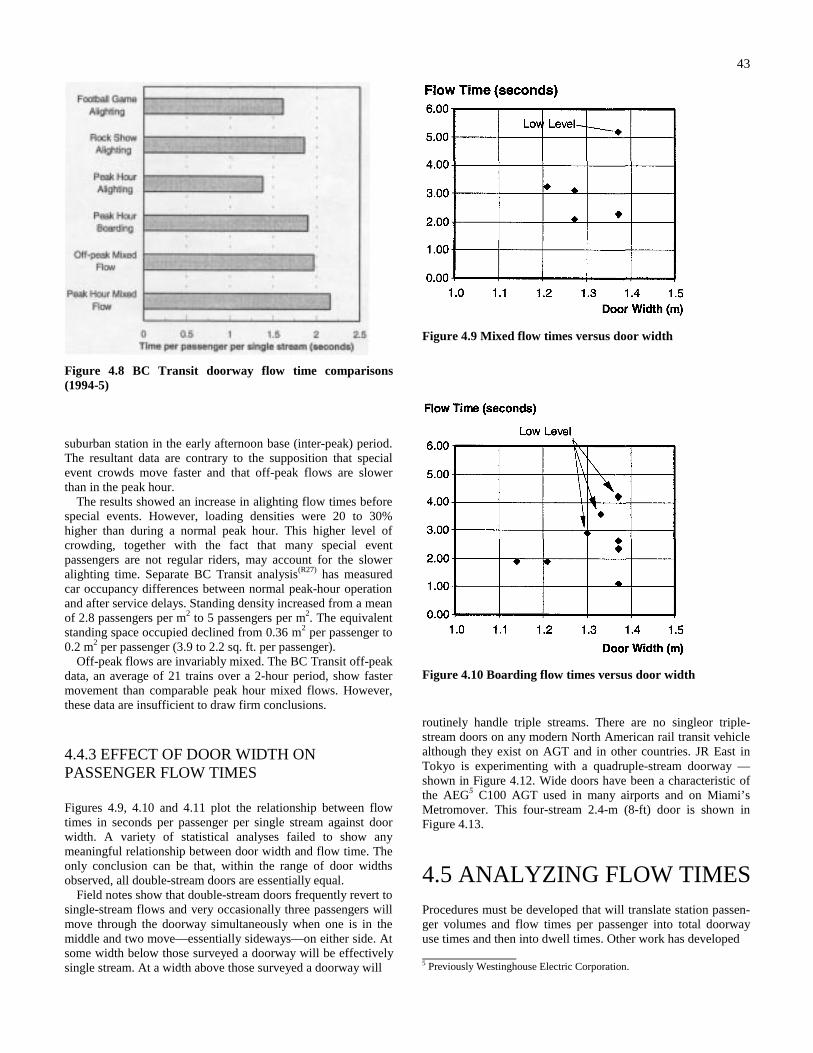
43

Figure 4.8 BC Transit doorway flow time comparisons(1994-5)

suburban station in the early afternoon base (inter-peak) period.The resultant data are contrary to the supposition that specialevent crowds move faster and that off-peak flows are slowerthan in the peak hour.

The results showed an increase in alighting flow times beforespecial events. However, loading densities were 20 to 30%higher than during a normal peak hour. This higher level ofcrowding, together with the fact that many special eventpassengers are not regular riders, may account for the sloweralighting time. Separate BC Transit analysis(R27) has measuredcar occupancy differences between normal peak-hour operationand after service delays. Standing density increased from a meanof 2.8 passengers per m2 to 5 passengers per m2. The equivalentstanding space occupied declined from 0.36 m2 per passenger to0.2 m2 per passenger (3.9 to 2.2 sq. ft. per passenger).

Off-peak flows are invariably mixed. The BC Transit off-peakdata, an average of 21 trains over a 2-hour period, show fastermovement than comparable peak hour mixed flows. However,these data are insufficient to draw firm conclusions.

4.4.3 EFFECT OF DOOR WIDTH ONPASSENGER FLOW TIMES

Figures 4.9, 4.10 and 4.11 plot the relationship between flowtimes in seconds per passenger per single stream against doorwidth. A variety of statistical analyses failed to show anymeaningful relationship between door width and flow time. Theonly conclusion can be that, within the range of door widthsobserved, all double-stream doors are essentially equal.

Field notes show that double-stream doors frequently revert tosingle-stream flows and very occasionally three passengers willmove through the doorway simultaneously when one is in themiddle and two move—essentially sideways—on either side. Atsome width below those surveyed a doorway will be effectivelysingle stream. At a width above those surveyed a doorway will

Figure 4.9 Mixed flow times versus door width

Figure 4.10 Boarding flow times versus door width

routinely handle triple streams. There are no singleor triple-stream doors on any modern North American rail transit vehiclealthough they exist on AGT and in other countries. JR East inTokyo is experimenting with a quadruple-stream doorway —shown in Figure 4.12. Wide doors have been a characteristic ofthe AEG5 C100 AGT used in many airports and on Miami’sMetromover. This four-stream 2.4-m (8-ft) door is shown inFigure 4.13.

4.5 ANALYZING FLOW TIMESProcedures must be developed that will translate station passen-ger volumes and flow times per passenger into total doorwayuse times and then into dwell times. Other work has developed 5 Previously Westinghouse Electric Corporation.

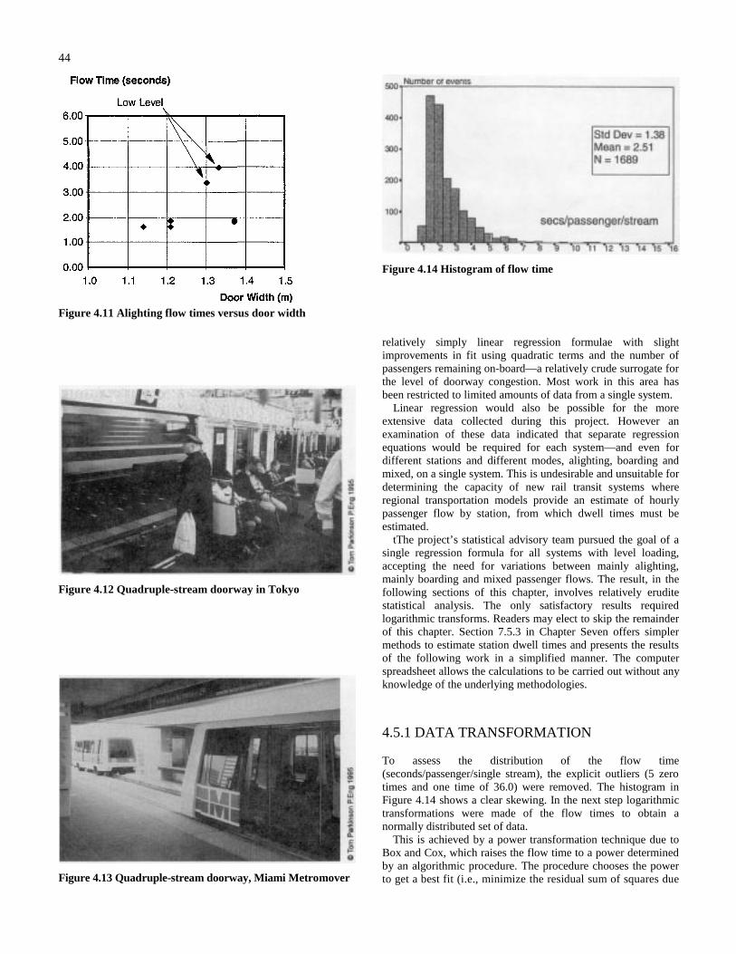
44

Figure 4.11 Alighting flow times versus door width

Figure 4.12 Quadruple-stream doorway in Tokyo

Figure 4.13 Quadruple-stream doorway, Miami Metromover

Figure 4.14 Histogram of flow time

relatively simply linear regression formulae with slightimprovements in fit using quadratic terms and the number ofpassengers remaining on-board—a relatively crude surrogate forthe level of doorway congestion. Most work in this area hasbeen restricted to limited amounts of data from a single system.

Linear regression would also be possible for the moreextensive data collected during this project. However anexamination of these data indicated that separate regressionequations would be required for each system—and even fordifferent stations and different modes, alighting, boarding andmixed, on a single system. This is undesirable and unsuitable fordetermining the capacity of new rail transit systems whereregional transportation models provide an estimate of hourlypassenger flow by station, from which dwell times must beestimated.

tThe project’s statistical advisory team pursued the goal of asingle regression formula for all systems with level loading,accepting the need for variations between mainly alighting,mainly boarding and mixed passenger flows. The result, in thefollowing sections of this chapter, involves relatively eruditestatistical analysis. The only satisfactory results requiredlogarithmic transforms. Readers may elect to skip the remainderof this chapter. Section 7.5.3 in Chapter Seven offers simplermethods to estimate station dwell times and presents the resultsof the following work in a simplified manner. The computerspreadsheet allows the calculations to be carried out without anyknowledge of the underlying methodologies.

4.5.1 DATA TRANSFORMATION

To assess the distribution of the flow time(seconds/passenger/single stream), the explicit outliers (5 zerotimes and one time of 36.0) were removed. The histogram inFigure 4.14 shows a clear skewing. In the next step logarithmictransformations were made of the flow times to obtain anormally distributed set of data.

This is achieved by a power transformation technique due toBox and Cox, which raises the flow time to a power determinedby an algorithmic procedure. The procedure chooses the powerto get a best fit (i.e., minimize the residual sum of squares due

45

Figure 4.15 Residual sum of squares

Figure 4.16 Expected flow time cumulative probabilitiesversus observed cumulative probabilities (abscissa)

to error) in a typical regression. The results of these calculationsare shown in Figure 4.15.

This graph indicates that a power of -0.25 or 0 is appropriate.For ease of interpretation a power of zero, which corresponds toa natural logarithm (ln) transform, is preferable. Furthercalculation shows that this transformation is statisticallywarranted. Confirmation of this decision can be seen bycomparing the normal probability plots obtained fromregressions of flow time and ln(flow time) against time of day,shown in Figure 4.16.

4.5.2 COMPARISONS

Box plots are the easiest way to visually compare the natural logtransformed flow time data between cities, time of day, loadinglevels and event types. These plots enable the researcher toquickly compare the central values (the mid box horizontal lineis the median) and gauge the spread of the data (the boxrepresents the interquartile range; i.e., the top is the 75thpercentile and the bottom is the 25th percentile).

Analysis of variance is used to examine differences in the

Table 4.4 Overall data set summary (seconds)

Table 4.5 System comparison summary ln(flow time(secs))

There are highly significant differences between the cities(p<0.0001) which are enumerated in the following table. An ‘x’indicates a difference significant at the 5 percent level betweenthe cities.

Table 4.6 Significant differences between systems

mean value of ln(flow time) between different levels of avariable (e.g., by system).

RESULTS

Overall Descriptive statistics for the overall data set are asfollows: where SD or Std Dev = standard deviation, No. =Number of observations or Cases, ln = natural logarithm.

City/system comparison In this comparison all data are usedand the descriptive statistics for the eight systems are as follows(Table 4.5): There are highly significant differences between thecities (p<0.0001), which are enumerated in the Table 4.6. An ‘x’indicates a difference significant at the 5 percent level betweenthe cities.

Alighting/boarding comparison All trains with greater than orequal to 70% boarding passengers were declared to be boarding

46

Table 4.7 Alighting/boarding comparison

The mean natural log of the flow time was significantly(p<0.0001) less for alighting.

Table 4.8 Time of day comparison ln(flow time (secs))

The morning mean natural log of the flow time was mildlysignificantly (p=0.02) higher than that in the afternoon.

Table 4.9 Loading level comparison ln(flow time (secs))

There were significant differences in the mean natural log of theflow times between each pair of loading levels (p<0.05).

Table 4.10 Event time comparison ln(flow time (secs))

The special event log flow time was significantly (p<0.0001)lower than that during normal peak time

and similarly those with greater than or equal to 70% alightingpassengers were declared to be alighting. This reduced the dataset to 1047 cases with descriptive statistics as follows (Table4.7): The mean natural log of the flow time was significantly(p<0.0001) less for alighting.

Time of day comparison All data were used in comparing amand pm natural log flow times. The descriptive statistics are asfollows (Table 4.8): The morning mean natural log of the flowtime was mildly significantly (p=0.02) higher than that in theafternoon.

Loading level comparison In order to have a homogeneousdataset for comparing the effect of boarding levels, attentionwas restricted to the SF Muni datasets. The followingdescriptive statistics were calculated (Table 4.9). There weresignificant differences in the mean natural log of the flow timesbetween each pair of loading levels (p<0.05).

Event Time Comparison In order to have a homogeneousdataset for the comparison of the normal and special event

times, attention was restricted to the Vancouver Sky Train(Table 4.10). The special event log flow time was significantly(p<0.0001) lower than that during normal peak times. Figures4.17 through 4.21 show the comparison box plots with thefollowing key.

4.5.3 PREDICTION OF DOOR MOVEMENTTIME USING BOARDING AND ALIGHTING

Preliminary regressions indicate that it is preferable to use thenatural logarithm of the door movement (DM) time. This isillustrated in Figure 4.22, where the normal plot for thetransformed DM time is much closer to the line of identity, thatindicates normality. So, as with the flow time, the naturallogarithm of the door movement time is modeled, and theresulting prediction is transformed back to the raw scale byexponentiation. There is evidence (p=0.02) that separate fits arewarranted for mainly boarding (i.e. > 70% boarding), mainlyalighting (i.e. > 70% alighting) and mixed.

A number of parameterizations and combinations of the twoindependent variables, number boarding (B) and numberalighting (A) are possible. The coefficients of determination forthe various models are shown in the following table. Thecoefficient represents the proportion of variation in the data thatis explained by the model. In addition to theseparameterizations, the natural logarithm of the numbersboarding and alighting were considered, and dummy variableswere used to model the levels resulting from a discretization ofthe variables. However, these latter approaches did not providebetter fits than those above and so were not considered further.

The models were applied to the overall dataset and the threemutually exclusive subsets of mainly boarding (i.e. > 70%boarding), mainly alighting (i.e. > 70% alighting) and mixed;results are shown in Table 4.11. From the table, it can be seenthat there are gains of up to 16% in the proportion of variationexplained by considering separate models for the subsets ofmainly boarding, mainly alighting and mixed. The gains inconsidering more complex models than the simple additivelinear model (Model 1) are less clear.

There is little gain from introducing a term for the interactionbetween the number boarding and the number alighting as inmodel 2. However, there is an approximate gain of 10 percent,resulting from the introduction of quadratic terms in model 3,but no further gain from adding an interaction to this as in model4. Similarly, there is no gain from higher order terms andinteractions, which also tend to make the prediction moreunstable. Hence the quadratic model (Model 3) is chosen as thebest fit, explaining 50% to 80% of the variation in the data.

Residual plots from the regression with this quadratic modelshow an inverse fanning indicating that the residuals areinversely proportional to the logarithms of the flow times. Whilethis could be transformed toward an identical error structure, inthe interests of parsimony, no reparameterization of thelogarithm of the flow time is attempted. The Durbin-Watsonstatistic ranges between 1.3 and 1.6 indicating significant first-order positive auto correlation among the residuals and sostandard errors for parameters and associated tests must beviewed with some caution.

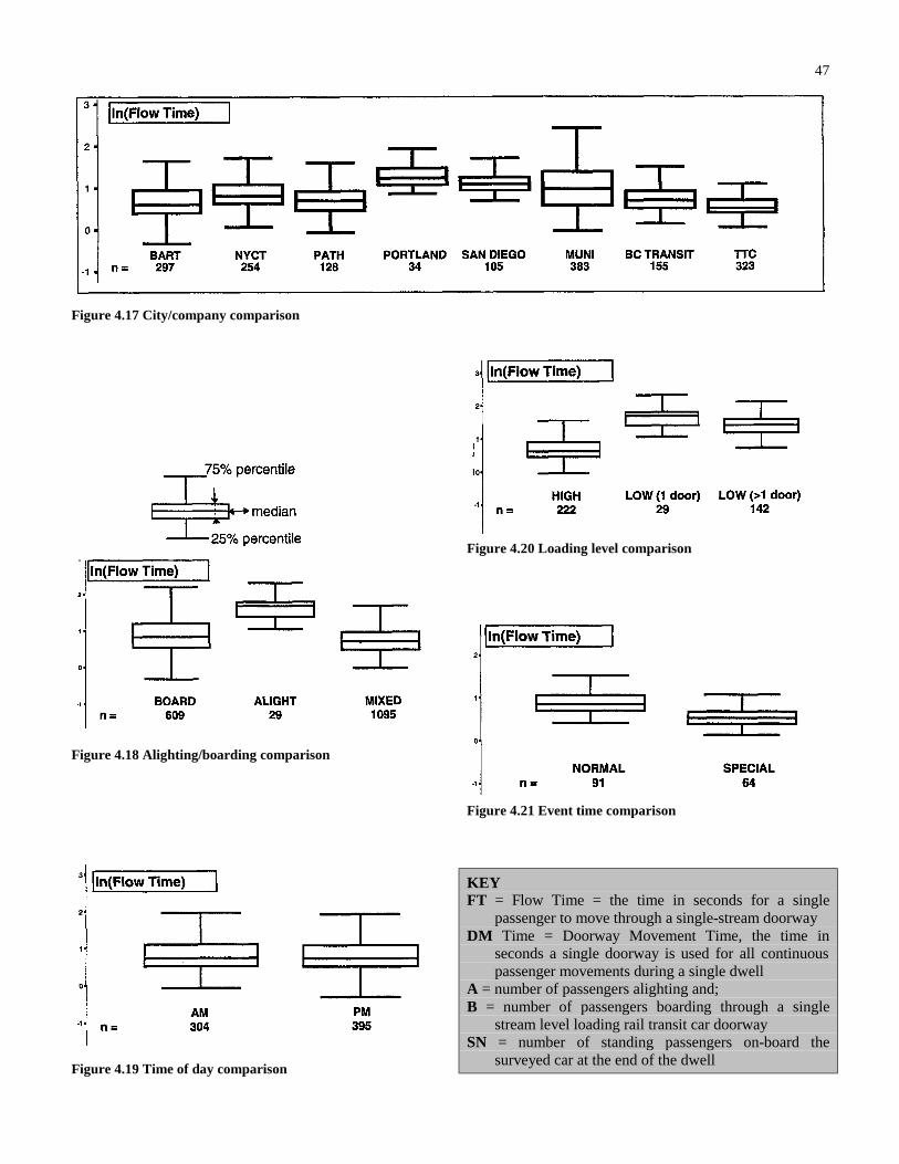
47

Figure 4.17 City/company comparison

Figure 4.18 Alighting/boarding comparison

Figure 4.19 Time of day comparison

Figure 4.20 Loading level comparison

Figure 4.21 Event time comparison

KEYFT = Flow Time = the time in seconds for a single

passenger to move through a single-stream doorwayDM Time = Doorway Movement Time, the time in

seconds a single doorway is used for all continuouspassenger movements during a single dwell

A = number of passengers alighting and;B = number of passengers boarding through a single

stream level loading rail transit car doorwaySN = number of standing passengers on-board the

surveyed car at the end of the dwell

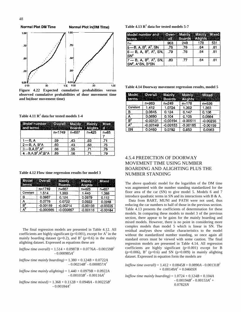
48

Figure 4.22 Expected cumulative probabilities versusobserved cumulative probabilities of door movement timeand ln(door movement time)

Table 4.11 R2 data for tested models 1-4

Table 4.12 Flow time regression results for model 3

The final regression models are presented in Table 4.12. Allcoefficients are highly significant (p<0.001), except for A2 in themainly boarding dataset (p=0.2), and B2 (p=0.6) in the mainlyalighting dataset. Expressed as equations these are

ln(flow time overall) = 1.514 + 0.0987B + 0.0776A - 0.00159B2

- 0.000985A2

ln(flow time mainly boarding) = 1.380 + 0.124B + 0.0722A- 0.00214B2 - 0.000857A2

ln(flow time mainly alighting) = 1.440 + 0.0979B + 0.0922A- 0.00103B2 - 0.00116A2

ln(flow time mixed) = 1.368 + 0.112B + 0.0948A - 0.00225B2

- 0.00184A2

Table 4.13 R2 data for tested models 5-7

Table 4.14 Doorway movement regression results, model 5

4.5.4 PREDICTION OF DOORWAYMOVEMENT TIME USING NUMBERBOARDING AND ALIGHTING PLUS THENUMBER STANDING

The above quadratic model for the logarithm of the DM timewas augmented with the number standing standardized for thefloor area of the car (SN) to give model 5. Models 6 and 7introduce quadratic terms in SN and its interactions with B & A.

Data from BART, MUNI and PATH were not used, thusreducing the car numbers to half of those in the previous section.Table 4.13 presents the coefficients of determination for thesemodels. In comparing these models to model 3 of the previoussection, there appear to be gains for the mainly boarding andmixed models. However, there is no point in considering morecomplex models than model 5 which is linear in SN. Theresidual analyses show similar characteristics to the modelwithout the standardized number standing, so once again allstandard errors must be viewed with some caution. The finalregression models are presented in Table 4.14. All regressioncoefficients are highly significant (p<0.001) except for B(p=0.006), B2 (p=0.6) and SN (p=0.009) in mainly alightingdataset. Expressed in equation form the models are

ln(flow time overall) = 1.412 + 0.0845B + 0.0890A - 0.00131B2

+ 0.00149A2 + 0.0460SN

ln(flow time mainly boarding) = 1.0724 + 0.124B + 0.104A- 0.00194B2 - 0.00153A2 +0.0782SN

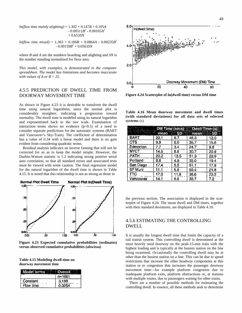
49

ln(flow time mainly alighting) = 1.302 + 0.147B + 0.105A- 0.00511B2 - 0.00165A2

+ 0.653SN

ln(flow time mixed) = 1.363 + 0.106B + 0.0864A - 0.00235B2

- 0.00159B2 + 0.0563SN

where B and A are the numbers boarding and alighting and SN isthe number standing normalized for floor area.

This model, with examples, is demonstrated in the computerspreadsheet. The model has limitations and becomes inaccuratewith values of A or B > 25.

4.5.5 PREDICTION OF DWELL TIME FROMDOORWAY MOVEMENT TIME

As shown in Figure 4.23 it is desirable to transform the dwelltime using natural logarithms, since the normal plot isconsiderably straighter, indicating a progression towardnormality. The dwell time is modeled using its natural logarithmand exponentiated back to the raw scale. Examination ofinteraction terms shows no evidence (p=0.5) of a need toconsider separate predictions for the automatic systems (BARTand Vancouver’s Sky-Train). The coefficient of determinationhas a value of 0.34 with a linear model and there is no gainevident from considering quadratic terms.

Residual analysis indicates an inverse fanning that will not becorrected for so as to keep the model simple. However, theDurbin-Watson statistic is 1.2 indicating strong positive serialauto correlation, so that all standard errors and associated testsmust be viewed with some caution. The final regression modelfor the natural logarithm of the dwell time is shown in Table4.15. It is noted that this relationship is not as strong as those in

Figure 4.23 Expected cumulative probabilities (ordinates)versus observed cumulative probabilities (abscissa)

Table 4.15 Modeling dwell time ondoorway movement time

Figure 4.24 Scatterplot of ln(dwell time) versus DM time

Table 4.16 Mean doorway movement and dwell times(with standard deviations) for all data sets of selectedsystems (s)

the previous section. The association is displayed in the scat-terplot of Figure 4.24. The mean dwell and DM times, togetherwith their standard deviations, are displayed in Table 4.16.

4.5.6 ESTIMATING THE CONTROLLINGDWELL

It is usually the longest dwell time that limits the capacity of arail transit system. This controlling dwell is determined at themost heavily used doorway on the peak-15-min train with thehighest loading and is typically at the busiest station on the linebeing examined. Occasionally the controlling dwell may be atother than the busiest station on a line. This can be due to speedrestrictions that increase the other headway components at thisstation or to congestion that increases the passenger doorwaymovement time—for example platform congestion due toinadequate platform exits, platform obstructions or, at stationswith multiple routes, due to passengers waiting for other trains.

There are a number of possible methods for estimating thecontrolling dwell. In essence, all these methods seek to determine

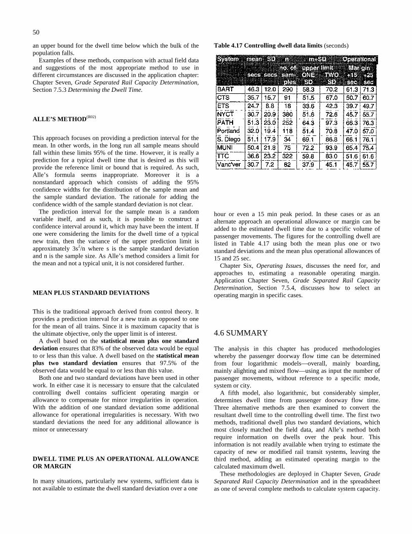
50

an upper bound for the dwell time below which the bulk of thepopulation falls.

Examples of these methods, comparison with actual field dataand suggestions of the most appropriate method to use indifferent circumstances are discussed in the application chapter:Chapter Seven, Grade Separated Rail Capacity Determination,Section 7.5.3 Determining the Dwell Time.

ALLE’S METHOD (R02)

This approach focuses on providing a prediction interval for themean. In other words, in the long run all sample means shouldfall within these limits 95% of the time. However, it is really aprediction for a typical dwell time that is desired as this willprovide the reference limit or bound that is required. As such,Alle’s formula seems inappropriate. Moreover it is anonstandard approach which consists of adding the 95%confidence widths for the distribution of the sample mean andthe sample standard deviation. The rationale for adding theconfidence width of the sample standard deviation is not clear.

The prediction interval for the sample mean is a randomvariable itself, and as such, it is possible to construct aconfidence interval around it, which may have been the intent. Ifone were considering the limits for the dwell time of a typicalnew train, then the variance of the upper prediction limit isapproximately 3s2/n where s is the sample standard deviationand n is the sample size. As Alle’s method considers a limit forthe mean and not a typical unit, it is not considered further.

MEAN PLUS STANDARD DEVIATIONS

This is the traditional approach derived from control theory. Itprovides a prediction interval for a new train as opposed to onefor the mean of all trains. Since it is maximum capacity that isthe ultimate objective, only the upper limit is of interest.

A dwell based on the statistical mean plus one standarddeviation ensures that 83% of the observed data would be equalto or less than this value. A dwell based on the statistical meanplus two standard deviation ensures that 97.5% of theobserved data would be equal to or less than this value.

Both one and two standard deviations have been used in otherwork. In either case it is necessary to ensure that the calculatedcontrolling dwell contains sufficient operating margin orallowance to compensate for minor irregularities in operation.With the addition of one standard deviation some additionalallowance for operational irregularities is necessary. With twostandard deviations the need for any additional allowance isminor or unnecessary

DWELL TIME PLUS AN OPERATIONAL ALLOWANCEOR MARGIN

In many situations, particularly new systems, sufficient data isnot available to estimate the dwell standard deviation over a one

Table 4.17 Controlling dwell data limits (seconds)

hour or even a 15 min peak period. In these cases or as analternate approach an operational allowance or margin can beadded to the estimated dwell time due to a specific volume ofpassenger movements. The figures for the controlling dwell arelisted in Table 4.17 using both the mean plus one or twostandard deviations and the mean plus operational allowances of15 and 25 sec.

Chapter Six, Operating Issues, discusses the need for, andapproaches to, estimating a reasonable operating margin.Application Chapter Seven, Grade Separated Rail CapacityDetermination, Section 7.5.4, discusses how to select anoperating margin in specific cases.

4.6 SUMMARY

The analysis in this chapter has produced methodologieswhereby the passenger doorway flow time can be determinedfrom four logarithmic models—overall, mainly boarding,mainly alighting and mixed flow—using as input the number ofpassenger movements, without reference to a specific mode,system or city.

A fifth model, also logarithmic, but considerably simpler,determines dwell time from passenger doorway flow time.Three alternative methods are then examined to convert theresultant dwell time to the controlling dwell time. The first twomethods, traditional dwell plus two standard deviations, whichmost closely matched the field data, and Alle’s method bothrequire information on dwells over the peak hour. Thisinformation is not readily available when trying to estimate thecapacity of new or modified rail transit systems, leaving thethird method, adding an estimated operating margin to thecalculated maximum dwell.

These methodologies are deployed in Chapter Seven, GradeSeparated Rail Capacity Determination and in the spreadsheetas one of several complete methods to calculate system capacity.

51

5. Passenger Loading Levels

5.1 INTRODUCTION

Establishing the loading level of rail transit is usually the finalstep in determining capacity—and one of the most variable.After the maximum train throughput has been calculated fromthe inverse of the sum of signaling separation time, dwell timeand operating margin, then capacity is based only on train lengthand loading level.

It is important to remember the feedback processes; that trainlength significantly changes the signaling separation time andthat loading levels affect dwell times.

The existing loading levels on North American rail transitvary from the relaxed seating of premium service (club cars)operated on specific trains of a few commuter rail lines to thedensest loading of an urban subway car in Mexico City—arange of 1.5 to 0.17 m2 per passenger (16 to 1.8 sq ft).

This wide range is more than eight to one. A more normalloading level range, discounting Mexico City and commuter rail,is two or three to one. This range makes the precisedetermination of loading level difficult. The main factor is apolicy issue, the question of relative comfort—heavilyrestrained by economic issues.

Notwithstanding Toronto’s subway and PATCO’sLindenwold line, the first new rail transit network in NorthAmerica in the last half century was BART. In the early 1960s,planning for this network—more a suburban railway than aninner-city subway—was based on the provision of a seat forevery passenger. Subsequently economic reality has forcedacceptance of standing passengers, particularly for shorter tripsin San Francisco and through the Transbay tube. Nevertheless,BART remains an example of a system that was designed to,and succeeded in, attracting passengers from alternate modes.

More so now, entering the twenty-first century, than 30 yearsago, rail transit is being planned as an alternative to theautomobile. While additions to existing systems can be expectedto follow existing standards, new systems have to determinetheir service standards. The principal standards include speed,frequency of service at peak and off-peak times—often termedpolicy headways—and loading levels. Schedule speed is fixedwhen the alignment, station spacing and equipmentspecifications are set; headways are usually closely tied todemand, although unmanned trains, as used on Vancouver’sSkyTrain and Miami’s Metromover, make short, frequent trainsover much of the day more affordable. Loading level is theremaining variable. Loading levels and headways interact asmore comfortable standards require either longer or morefrequent trains.

Demery(R22) states:

Long before crowding levels......reached New Yorklevels, prospective passengers would choose to travelby a different route, by a different mode, at a differenttime, or not at all.

and

Outside the largest, most congested urban areas, thelevel of crowding that transit passengers appearwilling to tolerate falls well short of theoretical“design” or “maximum” vehicle capacity.

These are important issues to consider in establishing loadingstandards.

In the next section, existing loading standards are reviewed.The remainder of the chapter determines a range of loadingstandards that can be applied in specific circumstances for eachmode.

It is possible to determine the interior dimensions of a railtransit vehicle; subtract the space taken up by cabs, equipmentand, for low-loading light rail, stairwells; then assign theresidual floor space to seated and standing passengers on thebasis of selected densities. This approach is one of severalfollowed in this chapter. However, the recommended method issimply to apply a passenger loading per unit of train length.

5.2 STANDARDS

A 1992 New York City Transit policy paper, Rapid TransitLoading Guidelines,(R48) gives the loading and service standardsthat have been applied, with minor modifications, to the NewYork subway system since 1987. The guidelines provide forslightly more space per passenger than those in effect until1986. Modifications have allowed for a relaxation in thenonrush hour passenger loading guideline to allow for theoperation of short trains.

The loading guidelines were established from test loadings ofdifferent car types, loading surveys of revenue service at thepeak load point and comparisons with the policies of other railtransit operators. Additional concerns such as passengercomfort, dwell time effects, uneven loading within trains, and anallowance for slack capacity in the event of service irregularitiesand fluctuations in passenger demand were also considered. Arush hour standard of 3 sq ft per standing passenger (3.6passengers per m2) was generated from this work. The policyrecognizes that this condition is only to be met at the maximumload point on a route and so is effective for only a short time andsmall portion of the overall route. For comparison, the agency’scalculations of the maximum capacity of each car type are basedon 6.6 - 6.8 passengers per m2.

Figure 5.1 compares the loading standards of the older NorthAmerican subway systems. NYCT standards for loading in thenonrush hours are more generous, with a seated load at themaximum load point being the general standard. If this wouldrequire headways of 4 min or less, or preclude operation of shorttrains, a standard of 125% of seated capacity applies. This

52

Figure 5.1 Scheduled loading guidelines (passengers/m2)

Figure 5.2 New York loading guidelines (passengers/m2)

Table 5.1 New York policy service levels

consideration of passenger comfort also extends to rush hourservice on lines where the headway is longer than 4 min. Inthese cases a sliding scale is used to ensure lower standingdensities on routes with longer headways, as shown in Figure5.2. Minimum headways for each day and service period areshown in Table 5.1. The NYCT standard of 3.6 passengers perm2 can be compared with the average occupancy into the CBDover the peak period as shown in Table 5.2. Table 5.3 tabulatesand compares daily and peak-hour ridership and passengers pervehicle for 19 New York CBD trunks for 1976 and 1991. Thisdecrease in NYCT car loadings partly reflected the improvement

Table 5.2 Passenger space on selected US systems(R22)

Table 5.3 Changes in NYCT peak-hour car loading(R22)

2 Average and Median include additional data sets.

in service standards of 1987, among other factors. Severaltrunks continue to operate at or near capacity.1

Care should be taken in comparing and applying the servicestandards with hourly average loadings. Service standards areusually based on the peak within the peak—15 min or less.

A loading diversity factor equating 15-min and peak-hourflows was introduced in Chapter One, Rail Transit In NorthAmerica. Section 5.6 of this chapter discusses the issues of load-ing diversity, provides data on existing factors by system andmode, and recommends factors for use in capacity calculations.The loading diversity factor for New York trunk routes, shown 1 Similar comparisons can be made for other cities and earlier years using

data from this report and from the TRB’s Highway Capacity Manual,Chapter 12 and appendices. Ridership and loading level information in theHCM are based on data to 1976 plus some historic data.(R67)

53

in Figure 5.3, ranges from 0.675 to 0.925 with an average of0.817. This diversity must be taken into account to determinepeak-hour capacity from a given service standard. NYCT’sstandard of 3.6 passengers per m2 over the peak-within-the-peakbecomes 3.6 × 0.82 or 2.95 (3.65 sq ft per passenger) onaverage, over the peak hour.

Outside New York the peak-within-the peak tends to be morepronounced and the peak-hour diversity factor is lower.3 In partthis is due to the long established Manhattan program to staggerwork hours and the natural tendency of passengers to avoid themost crowded period—particularly on lines that are close tocapacity.

Space occupancy during the peak period on other NorthAmerican rail transit systems varies widely from below 0.3passengers per m2 (3.2 sq ft) to over 1.0 m2 (11 sq ft) on somecommuter rail lines, as shown in Figure 5.4. Note that thehighest capacity entry (labeled NYCT) represents two tracksthat combine local and express service.

In analyzing this data Pushkarev et al.(R51) suggest a standardof 0.5 m2 (5.4 sq ft) per passenger. This will be discussed in thenext section. In addition to standards or policies for themaximum loading on peak-within-the-peak trains and forminimum headways (policy headways) at off-peak times, someoperators specify a maximum standing time. This is more oftena goal rather than a specific standard—20 min is typical.

Commuter Rail Loading levels for commuter rail are uniqueand uniform. Although standing passengers may be accepted forshort inner-city stretches or during times of serviceirregularities, the policy is to provide a seat for all passengers.Capacity is usually cited at 90 to 95% of the number of seats onthe train.

5.3 SPACE REQUIREMENTSThe surveyed literature contains many references to passengerspace requirements. The Batelle Institute(R12) recommendscomfort levels for public transport vehicles. The passengerstanding density recommendations are

• COMFORTABLE 2-3 passengers per m2

• UNCOMFORTABLE 5 passengers per m2

• UNACCEPTABLE >8 passengers per m2

In contrast, Pushkarev et al.(R51), suggesting gross vehicle floorarea as a readily available measure of car occupancy,recommends the following standards:

• ADEQUATE 0.5 m2—provides comfortable capacity perpassenger space

• TOLERABLE WITH DIFFICULTY 0.35 m2—lower limitin North America with “some touching”

• TOTALLY INTOLERABLE 0.2 m2—least amount ofspace that is occasionally accepted

Batelle(R12) also provides details of the projected body space ofpassengers in various situations. The most useful of these for 3 Shown in Chapter One, Figures 1.4 and 1.6.

Figure 5.3 15-min peak-within-the-peak compared to fullpeak-hour ridership on New York subway trunks

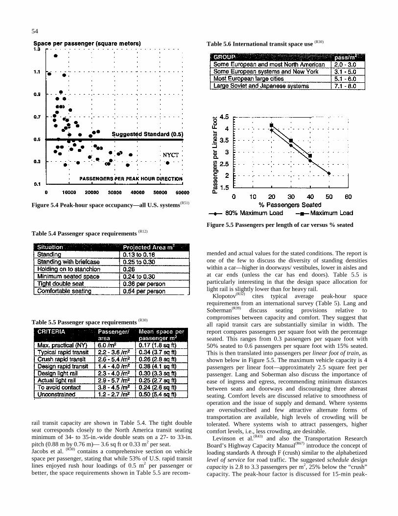
54

Figure 5.4 Peak-hour space occupancy—all U.S. systems(R51)

Table 5.4 Passenger space requirements (R12)

Table 5.5 Passenger space requirements (R30)

rail transit capacity are shown in Table 5.4. The tight doubleseat corresponds closely to the North America transit seatingminimum of 34- to 35-in.-wide double seats on a 27- to 33-in.pitch (0.88 m by 0.76 m)— 3.6 sq ft or 0.33 m2 per seat.Jacobs et al. (R30) contains a comprehensive section on vehiclespace per passenger, stating that while 53% of U.S. rapid transitlines enjoyed rush hour loadings of 0.5 m2 per passenger orbetter, the space requirements shown in Table 5.5 are recom-

Table 5.6 International transit space use (R30)

Figure 5.5 Passengers per length of car versus % seated

mended and actual values for the stated conditions. The report isone of the few to discuss the diversity of standing densitieswithin a car—higher in doorways/ vestibules, lower in aisles andat car ends (unless the car has end doors). Table 5.5 isparticularly interesting in that the design space allocation forlight rail is slightly lower than for heavy rail.

Klopotov(R32) cites typical average peak-hour spacerequirements from an international survey (Table 5). Lang andSoberman(R39) discuss seating provisions relative tocompromises between capacity and comfort. They suggest thatall rapid transit cars are substantially similar in width. Thereport compares passengers per square foot with the percentageseated. This ranges from 0.3 passengers per square foot with50% seated to 0.6 passengers per square foot with 15% seated.This is then translated into passengers per linear foot of train, asshown below in Figure 5.5. The maximum vehicle capacity is 4passengers per linear foot—approximately 2.5 square feet perpassenger. Lang and Soberman also discuss the importance ofease of ingress and egress, recommending minimum distancesbetween seats and doorways and discouraging three abreastseating. Comfort levels are discussed relative to smoothness ofoperation and the issue of supply and demand. Where systemsare oversubscribed and few attractive alternate forms oftransportation are available, high levels of crowding will betolerated. Where systems wish to attract passengers, highercomfort levels, i.e., less crowding, are desirable.

Levinson et al.(R43) and also the Transportation ResearchBoard’s Highway Capacity Manual(R67) introduce the concept ofloading standards A through F (crush) similar to the alphabetizedlevel of service for road traffic. The suggested schedule designcapacity is 2.8 to 3.3 passengers per m2, 25% below the “crush”capacity. The peak-hour factor is discussed for 15-min peak-

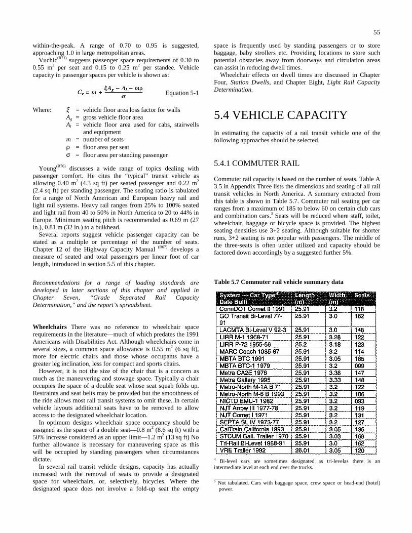
55

within-the-peak. A range of 0.70 to 0.95 is suggested,approaching 1.0 in large metropolitan areas.

Vuchic(R71) suggests passenger space requirements of 0.30 to0.55 m2 per seat and 0.15 to 0.25 m2 per standee. Vehiclecapacity in passenger spaces per vehicle is shown as:

Equation 5-1

Where: ξ = vehicle floor area loss factor for wallsAg = gross vehicle floor areaAl = vehicle floor area used for cabs, stairwells

and equipmentm = number of seatsρ = floor area per seatσ = floor area per standing passenger

Young(R76) discusses a wide range of topics dealing withpassenger comfort. He cites the “typical” transit vehicle asallowing 0.40 m2 (4.3 sq ft) per seated passenger and 0.22 m2

(2.4 sq ft) per standing passenger. The seating ratio is tabulatedfor a range of North American and European heavy rail andlight rail systems. Heavy rail ranges from 25% to 100% seatedand light rail from 40 to 50% in North America to 20 to 44% inEurope. Minimum seating pitch is recommended as 0.69 m (27in.), 0.81 m (32 in.) to a bulkhead.

Several reports suggest vehicle passenger capacity can bestated as a multiple or percentage of the number of seats.Chapter 12 of the Highway Capacity Manual (R67) develops ameasure of seated and total passengers per linear foot of carlength, introduced in section 5.5 of this chapter.

Recommendations for a range of loading standards aredeveloped in later sections of this chapter and applied inChapter Seven, “Grade Separated Rail CapacityDetermination,” and the report’s spreadsheet.

Wheelchairs There was no reference to wheelchair spacerequirements in the literature—much of which predates the 1991Americans with Disabilities Act. Although wheelchairs come inseveral sizes, a common space allowance is 0.55 m2 (6 sq ft),more for electric chairs and those whose occupants have agreater leg inclination, less for compact and sports chairs.

However, it is not the size of the chair that is a concern asmuch as the maneuvering and stowage space. Typically a chairoccupies the space of a double seat whose seat squab folds up.Restraints and seat belts may be provided but the smoothness ofthe ride allows most rail transit systems to omit these. In certainvehicle layouts additional seats have to be removed to allowaccess to the designated wheelchair location.

In optimum designs wheelchair space occupancy should beassigned as the space of a double seat—0.8 m2 (8.6 sq ft) with a50% increase considered as an upper limit—1.2 m2 (13 sq ft) Nofurther allowance is necessary for maneuvering space as thiswill be occupied by standing passengers when circumstancesdictate.

In several rail transit vehicle designs, capacity has actuallyincreased with the removal of seats to provide a designatedspace for wheelchairs, or, selectively, bicycles. Where thedesignated space does not involve a fold-up seat the empty

space is frequently used by standing passengers or to storebaggage, baby strollers etc. Providing locations to store suchpotential obstacles away from doorways and circulation areascan assist in reducing dwell times.

Wheelchair effects on dwell times are discussed in ChapterFour, Station Dwells, and Chapter Eight, Light Rail CapacityDetermination.

5.4 VEHICLE CAPACITYIn estimating the capacity of a rail transit vehicle one of thefollowing approaches should be selected.

5.4.1 COMMUTER RAIL

Commuter rail capacity is based on the number of seats. Table A3.5 in Appendix Three lists the dimensions and seating of all railtransit vehicles in North America. A summary extracted fromthis table is shown in Table 5.7. Commuter rail seating per carranges from a maximum of 185 to below 60 on certain club carsand combination cars.5 Seats will be reduced where staff, toilet,wheelchair, baggage or bicycle space is provided. The highestseating densities use 3+2 seating. Although suitable for shorterruns, 3+2 seating is not popular with passengers. The middle ofthe three-seats is often under utilized and capacity should befactored down accordingly by a suggested further 5%.

Table 5.7 Commuter rail vehicle summary data

4 Bi-level cars are sometimes designated as tri-levelas there is anintermediate level at each end over the trucks.

5 Not tabulated. Cars with baggage space, crew space or head-end (hotel)

power.

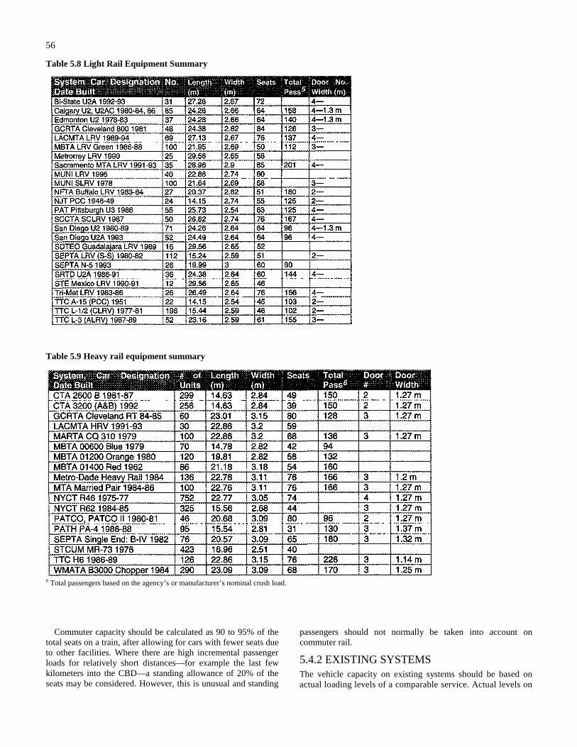
56

Table 5.8 Light Rail Equipment Summary

Table 5.9 Heavy rail equipment summary

6 Total passengers based on the agency’s or manufacturer’s nominal crush load.

Commuter capacity should be calculated as 90 to 95% of thetotal seats on a train, after allowing for cars with fewer seats dueto other facilities. Where there are high incremental passengerloads for relatively short distances—for example the last fewkilometers into the CBD—a standing allowance of 20% of theseats may be considered. However, this is unusual and standing

passengers should not normally be taken into account oncommuter rail.

5.4.2 EXISTING SYSTEMSThe vehicle capacity on existing systems should be based onactual loading levels of a comparable service. Actual levels on

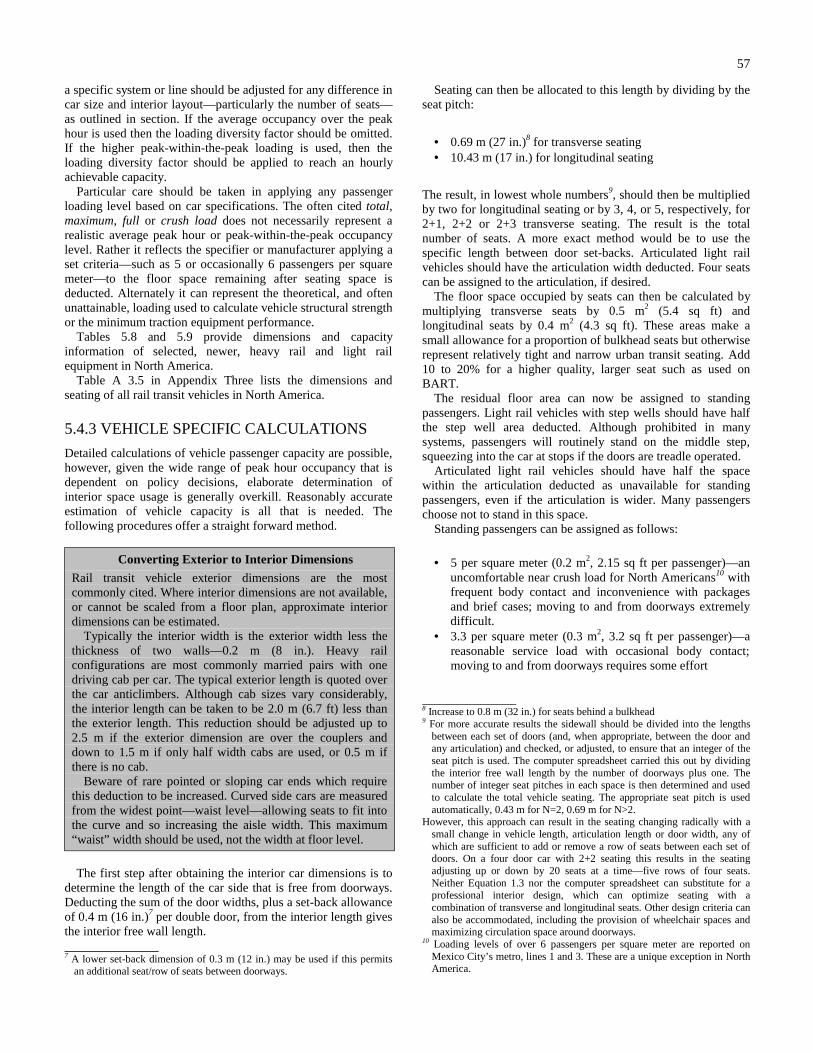
57

a specific system or line should be adjusted for any difference incar size and interior layout—particularly the number of seats—as outlined in section. If the average occupancy over the peakhour is used then the loading diversity factor should be omitted.If the higher peak-within-the-peak loading is used, then theloading diversity factor should be applied to reach an hourlyachievable capacity.

Particular care should be taken in applying any passengerloading level based on car specifications. The often cited total,maximum, full or crush load does not necessarily represent arealistic average peak hour or peak-within-the-peak occupancylevel. Rather it reflects the specifier or manufacturer applying aset criteria—such as 5 or occasionally 6 passengers per squaremeter—to the floor space remaining after seating space isdeducted. Alternately it can represent the theoretical, and oftenunattainable, loading used to calculate vehicle structural strengthor the minimum traction equipment performance.

Tables 5.8 and 5.9 provide dimensions and capacityinformation of selected, newer, heavy rail and light railequipment in North America.

Table A 3.5 in Appendix Three lists the dimensions andseating of all rail transit vehicles in North America.

5.4.3 VEHICLE SPECIFIC CALCULATIONS

Detailed calculations of vehicle passenger capacity are possible,however, given the wide range of peak hour occupancy that isdependent on policy decisions, elaborate determination ofinterior space usage is generally overkill. Reasonably accurateestimation of vehicle capacity is all that is needed. Thefollowing procedures offer a straight forward method.

Converting Exterior to Interior Dimensions

Rail transit vehicle exterior dimensions are the mostcommonly cited. Where interior dimensions are not available,or cannot be scaled from a floor plan, approximate interiordimensions can be estimated.

Typically the interior width is the exterior width less thethickness of two walls—0.2 m (8 in.). Heavy railconfigurations are most commonly married pairs with onedriving cab per car. The typical exterior length is quoted overthe car anticlimbers. Although cab sizes vary considerably,the interior length can be taken to be 2.0 m (6.7 ft) less thanthe exterior length. This reduction should be adjusted up to2.5 m if the exterior dimension are over the couplers anddown to 1.5 m if only half width cabs are used, or 0.5 m ifthere is no cab.

Beware of rare pointed or sloping car ends which requirethis deduction to be increased. Curved side cars are measuredfrom the widest point—waist level—allowing seats to fit intothe curve and so increasing the aisle width. This maximum“waist” width should be used, not the width at floor level.

The first step after obtaining the interior car dimensions is todetermine the length of the car side that is free from doorways.Deducting the sum of the door widths, plus a set-back allowanceof 0.4 m (16 in.)7 per double door, from the interior length givesthe interior free wall length. 7 A lower set-back dimension of 0.3 m (12 in.) may be used if this permits

an additional seat/row of seats between doorways.

Seating can then be allocated to this length by dividing by theseat pitch:

• 0.69 m (27 in.)8 for transverse seating• 10.43 m (17 in.) for longitudinal seating

The result, in lowest whole numbers9, should then be multipliedby two for longitudinal seating or by 3, 4, or 5, respectively, for2+1, 2+2 or 2+3 transverse seating. The result is the totalnumber of seats. A more exact method would be to use thespecific length between door set-backs. Articulated light railvehicles should have the articulation width deducted. Four seatscan be assigned to the articulation, if desired.

The floor space occupied by seats can then be calculated bymultiplying transverse seats by 0.5 m2 (5.4 sq ft) andlongitudinal seats by 0.4 m2 (4.3 sq ft). These areas make asmall allowance for a proportion of bulkhead seats but otherwiserepresent relatively tight and narrow urban transit seating. Add10 to 20% for a higher quality, larger seat such as used onBART.

The residual floor area can now be assigned to standingpassengers. Light rail vehicles with step wells should have halfthe step well area deducted. Although prohibited in manysystems, passengers will routinely stand on the middle step,squeezing into the car at stops if the doors are treadle operated.

Articulated light rail vehicles should have half the spacewithin the articulation deducted as unavailable for standingpassengers, even if the articulation is wider. Many passengerschoose not to stand in this space.

Standing passengers can be assigned as follows:

• 5 per square meter (0.2 m2, 2.15 sq ft per passenger)—anuncomfortable near crush load for North Americans10 withfrequent body contact and inconvenience with packagesand brief cases; moving to and from doorways extremelydifficult.

• 3.3 per square meter (0.3 m2, 3.2 sq ft per passenger)—areasonable service load with occasional body contact;moving to and from doorways requires some effort

8 Increase to 0.8 m (32 in.) for seats behind a bulkhead9 For more accurate results the sidewall should be divided into the lengths

between each set of doors (and, when appropriate, between the door andany articulation) and checked, or adjusted, to ensure that an integer of theseat pitch is used. The computer spreadsheet carried this out by dividingthe interior free wall length by the number of doorways plus one. Thenumber of integer seat pitches in each space is then determined and usedto calculate the total vehicle seating. The appropriate seat pitch is usedautomatically, 0.43 m for N=2, 0.69 m for N>2.

However, this approach can result in the seating changing radically with asmall change in vehicle length, articulation length or door width, any ofwhich are sufficient to add or remove a row of seats between each set ofdoors. On a four door car with 2+2 seating this results in the seatingadjusting up or down by 20 seats at a time—five rows of four seats.Neither Equation 1.3 nor the computer spreadsheet can substitute for aprofessional interior design, which can optimize seating with acombination of transverse and longitudinal seats. Other design criteria canalso be accommodated, including the provision of wheelchair spaces andmaximizing circulation space around doorways.

10 Loading levels of over 6 passengers per square meter are reported onMexico City’s metro, lines 1 and 3. These are a unique exception in NorthAmerica.

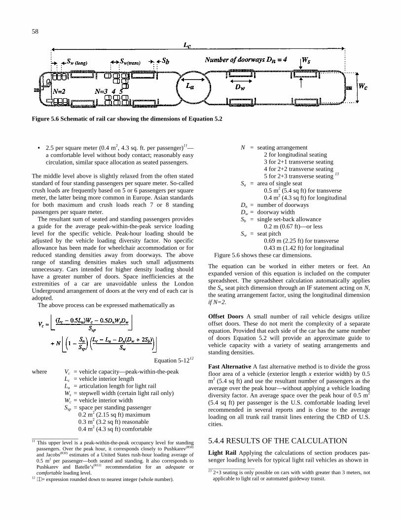
58

Figure 5.6 Schematic of rail car showing the dimensions of Equation 5.2

• 2.5 per square meter (0.4 m2, 4.3 sq. ft. per passenger)11—a comfortable level without body contact; reasonably easycirculation, similar space allocation as seated passengers.

The middle level above is slightly relaxed from the often statedstandard of four standing passengers per square meter. So-calledcrush loads are frequently based on 5 or 6 passengers per squaremeter, the latter being more common in Europe. Asian standardsfor both maximum and crush loads reach 7 or 8 standingpassengers per square meter.

The resultant sum of seated and standing passengers providesa guide for the average peak-within-the-peak service loadinglevel for the specific vehicle. Peak-hour loading should beadjusted by the vehicle loading diversity factor. No specificallowance has been made for wheelchair accommodation or forreduced standing densities away from doorways. The aboverange of standing densities makes such small adjustmentsunnecessary. Cars intended for higher density loading shouldhave a greater number of doors. Space inefficiencies at theextremities of a car are unavoidable unless the LondonUnderground arrangement of doors at the very end of each car isadopted.

The above process can be expressed mathematically as

Equation 5-1212

where Vc = vehicle capacity—peak-within-the-peakLc = vehicle interior lengthLa = articulation length for light railWs = stepwell width (certain light rail only)Wc = vehicle interior widthSsp = space per standing passenger

0.2 m2 (2.15 sq ft) maximum0.3 m2 (3.2 sq ft) reasonable0.4 m2 (4.3 sq ft) comfortable

11 This upper level is a peak-within-the-peak occupancy level for standing

passengers. Over the peak hour, it corresponds closely to Pushkarev(R50)

and Jacobs(R30) estimates of a United States rush-hour loading average of0.5 m2 per passenger—both seated and standing. It also corresponds toPushkarev and Batelle’s(R12) recommendation for an adequate orcomfortable loading level.

12 = expression rounded down to nearest integer (whole number).

N = seating arrangement2 for longitudinal seating3 for 2+1 transverse seating4 for 2+2 transverse seating5 for 2+3 transverse seating 13

Sa = area of single seat0.5 m2 (5.4 sq ft) for transverse0.4 m2 (4.3 sq ft) for longitudinal

Dn = number of doorwaysDw = doorway widthSb = single set-back allowance

0.2 m (0.67 ft)—or lessSw = seat pitch

0.69 m (2.25 ft) for transverse0.43 m (1.42 ft) for longitudinal

Figure 5.6 shows these car dimensions.

The equation can be worked in either meters or feet. Anexpanded version of this equation is included on the computerspreadsheet. The spreadsheet calculation automatically appliesthe Sw seat pitch dimension through an IF statement acting on N,the seating arrangement factor, using the longitudinal dimensionif N=2.

Offset Doors A small number of rail vehicle designs utilizeoffset doors. These do not merit the complexity of a separateequation. Provided that each side of the car has the same numberof doors Equation 5.2 will provide an approximate guide tovehicle capacity with a variety of seating arrangements andstanding densities.

Fast Alternative A fast alternative method is to divide the grossfloor area of a vehicle (exterior length x exterior width) by 0.5m2 (5.4 sq ft) and use the resultant number of passengers as theaverage over the peak hour—without applying a vehicle loadingdiversity factor. An average space over the peak hour of 0.5 m2

(5.4 sq ft) per passenger is the U.S. comfortable loading levelrecommended in several reports and is close to the averageloading on all trunk rail transit lines entering the CBD of U.S.cities.

5.4.4 RESULTS OF THE CALCULATION

Light Rail Applying the calculations of section produces pas-senger loading levels for typical light rail vehicles as shown in 13 2+3 seating is only possible on cars with width greater than 3 meters, not

applicable to light rail or automated guideway transit.

59

Table 5.10 Calculated light rail vehicle capacity

Table 5.11 Calculated heavy rail vehicle capacity

Table 5.10. Two articulated light rail vehicles are shown, thecommon Siemens-Düwag car used in nine systems (with somedimensional changes) and the largest North American light railvehicle used by the MTA in Baltimore. The resulting capacitiesare for a generic version of these cars. Reference to Table 5.9,Light Rail Equipment Summary, shows that the actual number ofseats in the Siemens-Düwag car varies from 52 to 72 while ratedtotal capacity varies from 96 to 201. This stresses the wide,policy related, car capacity issue.

The calculation cannot encompass all options. However, thecalculation provides a policy surrogate in the form of theallocated standing space,—0.2, 0.3 or 0.4 m2 per passenger.Seating should be adjusted accordingly. A need for highstanding levels would suggest longitudinal seats, low standinglevels, the 2+2 transverse seats.

Heavy Rail Applying the calculations of section producespassenger loading levels for typical heavy rail vehicles as shownin Table 5.11. Data is shown for a generic 23 meter heavy railcar with variations of seating arrangements and standing space

allocations. Two data sets follow for the smaller cars used inVancouver and Chicago.

5.5 LENGTHIn this section the above calculations are converted to thepassengers per unit length method suggested by Lang andSoberman(R39) and others, stratified into classes, then comparedwith actual peak-within-the-peak loading levels of NorthAmerican rail transit. Given the variation in loading levels thatdepend on policy—the standing density used and seat spacing—this simplified method is appropriate in most circumstances. It isthe recommended method of estimating peak-within-the-peakcar capacity except for circumstances and rolling stock that areout of the ordinary.

Light Rail Applying the calculations of section produces pas-senger loading levels for typical light rail vehicles as shown in

60

Figure 5.7 Linear passenger loading of articulated LRVs

Figure 5.8 Linear passenger loading of heavy rail cars

Table 5.10 and as passengers per unit length in Figure 5.7. Aswould be expected, the wider and longer Baltimore car hasproportionately higher loadings per meter of length. The typicalSiemens-Düwag car used on nine systems (with somedimensional changes) has a range of 5.0 to 8.0 passengers permeter of car length. The lower level of five passengers per meterlength—with a standing space per passenger of 0.4 m2—corresponds closely with the recommended quality loading of aan average of 0.5 m2 per passenger.

Heavy Rail Applying the calculations of section 5.4.3 producespassenger loading levels for typical heavy rail vehicles as shownin Table 5.11 and, as passengers per unit length, in Figure 5.8.As would be expected, the smaller and narrower cars inVancouver and Chicago have lower loadings per meter length.

The more generic 23-m-long cars used in over 12 NorthAmerican cities have a remarkably close data set for each of the

three variations, 4 and 3 door versions, and transverse orlongitudinal seating—with a range of 7.0 to 11.5 passengers permeter of car length. The lower end of the range of seven to eightpassengers per meter length—with a standing space perpassenger of 0.4 to 0.3 m2—is an appropriate range for higheruse systems. A lower figure of six corresponds closely with therecommended quality loading of an average of 0.5 square metersper passenger and is appropriate for a higher level of service onnew systems. In both cases a reduction by one should be usedfor smaller, narrower cars.

These calculated linear loading levels can be compared withactual levels on major North American rail transit lines shown inTable 5.12 and summarized in Table 5.13.

Heavy Rail outside New York shows a level comparable withthe recommended comfortable level of 6 passengers per meterof train length. New York is higher by some 25%, averaged over11 trunk routes. Commuter rail, with most passengers seated,has an average only 13% lower than the average of heavy railoutside New York. Only two light rail lines are running close tocapacity and peak-within-the-peak ridership is not available forthese.

5.6 LOADING DIVERSITY

Passengers do not load evenly into cars and trains over the peakhour. This unevenness is the diversity of passenger loading.There are three different types of loading diversity: unevennessof passenger loading within a car; unevenness of passengerloading within cars of a train; unevenness of passenger loadingwithin peak-hour trains. The loading diversity factor developedin this section essentially encompasses all three.

In individual cars, the highest standing densities occur arounddoorways, the lowest at the ends of the cars. Several Europeanurban rail systems add doors, sometimes only single stream, atthe car ends to reduce this unevenness. London Transport’sunderground system is the most notable with this feature onmost rolling stock,14 except at car ends with a driving cab. Theend door on the low-profile cars are 0.75 m (2.5 ft) widecompared to the main doors of 1.56 m (5.1 ft). Theseexceptionally wide doors, with their 0.17 m (6.8 in) set-backsoften accommodate three streams of passengers.

No data exist to determine such loading diversity within a carand the variations are accommodated in the average loadings ofthe previous sections. It is important in cars designed for highoccupancies to minimize this effect by using wide aisles,uncluttered vestibules and suitable hand holds that encouragepassengers to move into the extremities of a car. Very littleinformation was found on car interior design efficiency in theliterature search with the exception of Young(R76) PassengerComfort in Urban Transit Vehicles.

A second level of diversity occurs in uneven loading amongcars of a train. This second level is also included in the averageloading data of the previous sections and in the applicationchapters. Cars that are closer to station exits and entrances willbe more heavily loaded than more remote cars. This inefficiencycan be minimized by staggering platform entrances and exits

14 London’s Docklands Light Railway does not have end doors.

61

Table 5.12 Passengers per unit train length, major North American trunks

Table 5.13 Summary of linear passenger loading (per meter)Additional passenger loading per unit length data are compiledin Tables 7.4, 7.5 and 7.6 of Chapter Seven.

between ends, centers and third points of the platforms. This isnot always possible or practiced. The busiest, most denselyoccupied rail lines in North America, lines 1, 2 and 3 of MexicoCity’s metro all have stations with center entrances/exits. Evenso, relatively even loading occurs both here, and on rail transitlines at or near capacity elsewhere, due to the duress factor thatencourages passengers to spread themselves along the platformduring heavily traveled times—or risk being unable to get on thenext arriving train.Few systems count passengers by individual cars when these arecrush loaded. This is difficult to do with any accuracy and theresults differ little from assigning a set full load to each car

Figure 5.9 Vancouver, Broadway Station inbound peak-hourpassenger distribution between cars of train. October 271994, 50 trains, 12,173 passengers

of a fully loaded train. Data are available from two Canadianproperties.

BC Transit operates four car trains on headways down to 90sec. Pass-ups are routine at the busiest suburban station, Broad-way with an end and two third-point entrances/exits. The relativeloading of the four cars is shown in Figure 5.9. The mainentrance/exit is provided with escalators and lies between the

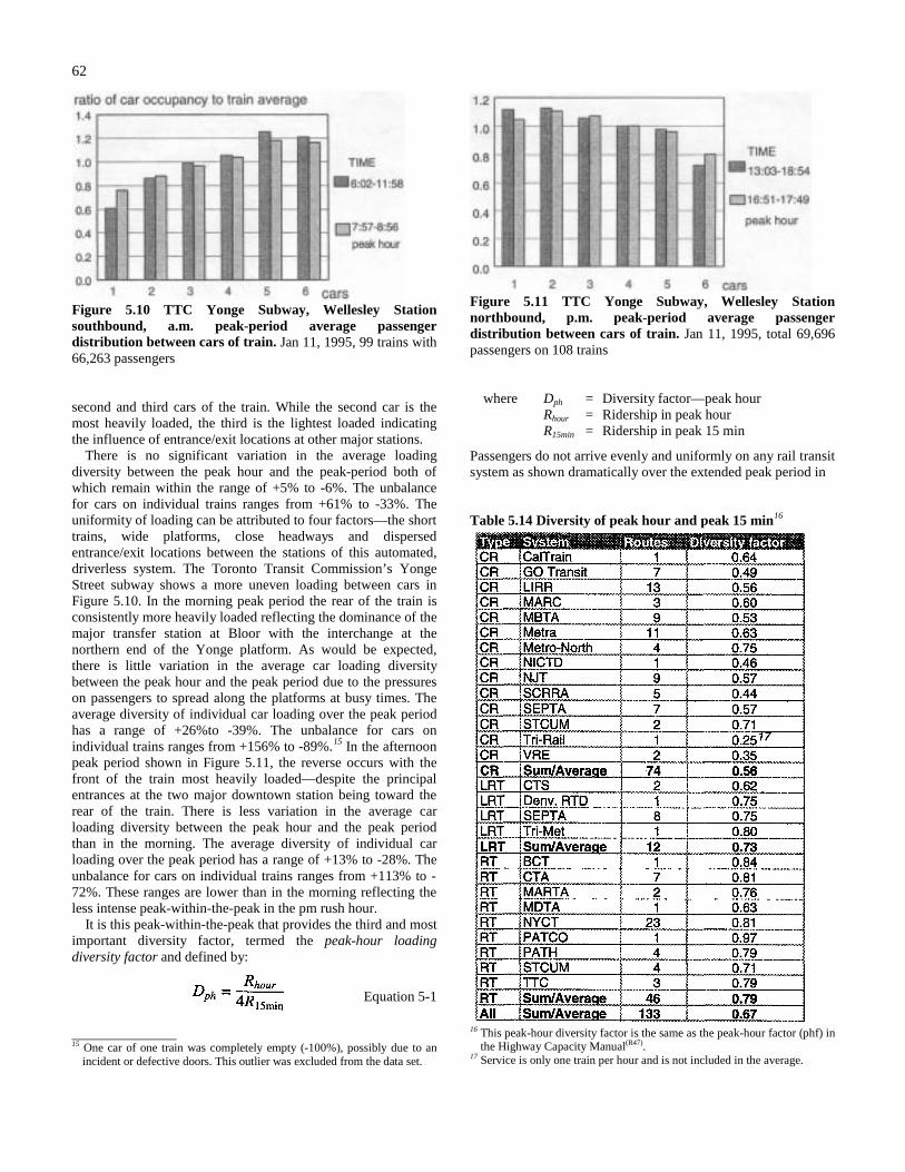
62

Figure 5.10 TTC Yonge Subway, Wellesley Stationsouthbound, a.m. peak-period average passengerdistribution between cars of train. Jan 11, 1995, 99 trains with66,263 passengers

second and third cars of the train. While the second car is themost heavily loaded, the third is the lightest loaded indicatingthe influence of entrance/exit locations at other major stations.

There is no significant variation in the average loadingdiversity between the peak hour and the peak-period both ofwhich remain within the range of +5% to -6%. The unbalancefor cars on individual trains ranges from +61% to -33%. Theuniformity of loading can be attributed to four factors—the shorttrains, wide platforms, close headways and dispersedentrance/exit locations between the stations of this automated,driverless system. The Toronto Transit Commission’s YongeStreet subway shows a more uneven loading between cars inFigure 5.10. In the morning peak period the rear of the train isconsistently more heavily loaded reflecting the dominance of themajor transfer station at Bloor with the interchange at thenorthern end of the Yonge platform. As would be expected,there is little variation in the average car loading diversitybetween the peak hour and the peak period due to the pressureson passengers to spread along the platforms at busy times. Theaverage diversity of individual car loading over the peak periodhas a range of +26%to -39%. The unbalance for cars onindividual trains ranges from +156% to -89%.15 In the afternoonpeak period shown in Figure 5.11, the reverse occurs with thefront of the train most heavily loaded—despite the principalentrances at the two major downtown station being toward therear of the train. There is less variation in the average carloading diversity between the peak hour and the peak periodthan in the morning. The average diversity of individual carloading over the peak period has a range of +13% to -28%. Theunbalance for cars on individual trains ranges from +113% to -72%. These ranges are lower than in the morning reflecting theless intense peak-within-the-peak in the pm rush hour.

It is this peak-within-the-peak that provides the third and mostimportant diversity factor, termed the peak-hour loadingdiversity factor and defined by:

Equation 5-1

15 One car of one train was completely empty (-100%), possibly due to an

incident or defective doors. This outlier was excluded from the data set.

Figure 5.11 TTC Yonge Subway, Wellesley Stationnorthbound, p.m. peak-period average passengerdistribution between cars of train. Jan 11, 1995, total 69,696passengers on 108 trains

where Dph = Diversity factor—peak hourRhour = Ridership in peak hourR15min = Ridership in peak 15 min

Passengers do not arrive evenly and uniformly on any rail transitsystem as shown dramatically over the extended peak period in

Table 5.14 Diversity of peak hour and peak 15 min16

16 This peak-hour diversity factor is the same as the peak-hour factor (phf) inthe Highway Capacity Manual(R47).

17 Service is only one train per hour and is not included in the average.

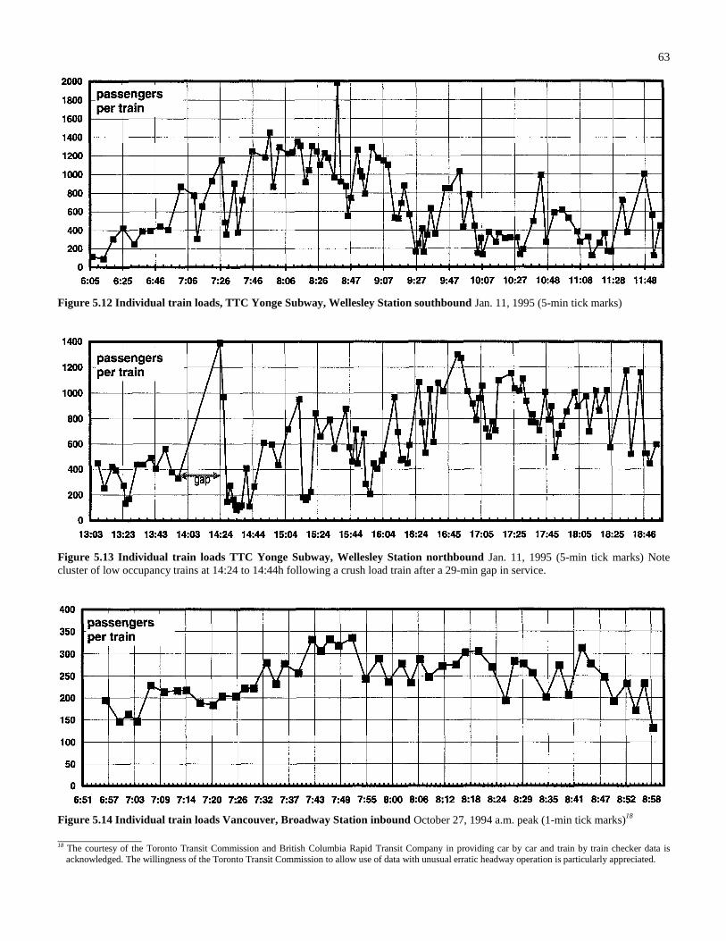
63

Figure 5.12 Individual train loads, TTC Yonge Subway, Wellesley Station southbound Jan. 11, 1995 (5-min tick marks)

Figure 5.13 Individual train loads TTC Yonge Subway, Wellesley Station northbound Jan. 11, 1995 (5-min tick marks) Notecluster of low occupancy trains at 14:24 to 14:44h following a crush load train after a 29-min gap in service.

Figure 5.14 Individual train loads Vancouver, Broadway Station inbound October 27, 1994 a.m. peak (1-min tick marks)18

18 The courtesy of the Toronto Transit Commission and British Columbia Rapid Transit Company in providing car by car and train by train checker data is

acknowledged. The willingness of the Toronto Transit Commission to allow use of data with unusual erratic headway operation is particularly appreciated.

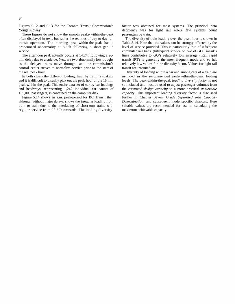
64

Figures 5.12 and 5.13 for the Toronto Transit Commission’sYonge subway.

These figures do not show the smooth peaks-within-the-peakoften displayed in texts but rather the realities of day-to-day railtransit operation. The morning peak-within-the-peak has apronounced abnormality at 8:35h following a short gap inservice.

The afternoon peak actually occurs at 14:24h following a 26-min delay due to a suicide. Next are two abnormally low troughsas the delayed trains move through—and the commission’scontrol center strives to normalize service prior to the start ofthe real peak hour.

In both charts the different loading, train by train, is strikingand it is difficult to visually pick out the peak hour or the 15 minpeak-within-the peak. This entire data set of car by car loadingsand headways, representing 1,242 individual car counts of135,000 passengers, is contained on the computer disk.

Figure 5.14 shows an a.m. peak-period for BC Transit that,although without major delays, shows the irregular loading fromtrain to train due to the interlacing of short-turn trains withregular service from 07:30h onwards. The loading diversity

factor was obtained for most systems. The principal datadeficiency was for light rail where few systems countpassengers by train.

The diversity of train loading over the peak hour is shown inTable 5.14. Note that the values can be strongly affected by thelevel of service provided. This is particularly true of infrequentcommuter rail lines. (Infrequent service on two of GO Transit’slines contributes to GO’s relatively low average.) Rail rapidtransit (RT) is generally the most frequent mode and so hasrelatively low values for the diversity factor. Values for light railtransit are intermediate.

Diversity of loading within a car and among cars of a train areincluded in the recommended peak-within-the-peak loadinglevels. The peak-within-the-peak loading diversity factor is notso included and must be used to adjust passenger volumes fromthe estimated design capacity to a more practical achievablecapacity. This important loading diversity factor is discussedfurther in Chapter Seven, Grade Separated Rail CapacityDetermination, and subsequent mode specific chapters. Heresuitable values are recommended for use in calculating themaximum achievable capacity.