1641 OptoTutorial SNAP PAC PIDdocuments.opto22.com/1641_OptoTutorial_SNAP_PAC_PID.pdfflowchart logic...
84
OPTOTUTORIAL: SNAP PAC PID A Supplement to the SNAP PAC Learning Center Form 1641-120824—August 2012 43044 Business Park Drive • Temecula • CA 92590-3614 Phone: 800-321-OPTO (6786) or 951-695-3000 Fax: 800-832-OPTO (6786) or 951-695-2712 www.opto22.com Product Support Services 800-TEK-OPTO (835-6786) or 951-695-3080 Fax: 951-695-3017 Email: [email protected] Web: support.opto22.com
Transcript of 1641 OptoTutorial SNAP PAC PIDdocuments.opto22.com/1641_OptoTutorial_SNAP_PAC_PID.pdfflowchart logic...
OPTOTUTORIAL: SNAP PAC PIDA Supplement to the SNAP PAC Learning Center
Form 1641-120824—August 2012
43044 Business Park Drive • Temecula • CA 92590-3614Phone: 800-321-OPTO (6786) or 951-695-3000
Fax: 800-832-OPTO (6786) or 951-695-2712www.opto22.com
Product Support Services800-TEK-OPTO (835-6786) or 951-695-3080
Fax: 951-695-3017Email: [email protected]
Web: support.opto22.com
OptoTutorial: SNAP PAC PIDii
OptoTutorial: SNAP PAC PIDForm 1641-120824—August 2012
Copyright © 2003–2012 Opto 22.All rights reserved.Printed in the United States of America.
The information in this manual has been checked carefully and is believed to be accurate; however, Opto 22 assumes no responsibility for possible inaccuracies or omissions. Specifications are subject to change without notice.
Opto 22 warrants all of its products to be free from defects in material or workmanship for 30 months from the manufacturing date code. This warranty is limited to the original cost of the unit only and does not cover installation, labor, or any other contingent costs. Opto 22 I/O modules and solid-state relays with date codes of 1/96 or later are guaranteed for life. This lifetime warranty excludes reed relay, SNAP serial communication modules, SNAP PID modules, and modules that contain mechanical contacts or switches. Opto 22 does not warrant any product, components, or parts not manufactured by Opto 22; for these items, the warranty from the original manufacturer applies. These products include, but are not limited to, OptoTerminal-G70, OptoTerminal-G75, and Sony Ericsson GT-48; see the product data sheet for specific warranty information. Refer to Opto 22 form number 1042 for complete warranty information.
Wired+Wireless controllers and brains and N-TRON wireless access points are licensed under one or more of the following patents: U.S. Patent No(s). 5282222, RE37802, 6963617; Canadian Patent No. 2064975; European Patent No. 1142245; French Patent No. 1142245; British Patent No. 1142245; Japanese Patent No. 2002535925A; German Patent No. 60011224.
Opto 22 FactoryFloor, Optomux, and Pamux are registered trademarks of Opto 22. Generation 4, ioControl, ioDisplay, ioManager, ioProject, ioUtilities, mistic, Nvio, Nvio.net Web Portal, OptoConnect, OptoControl, OptoDataLink, OptoDisplay, OptoEMU, OptoEMU Sensor, OptoEMU Server, OptoOPCServer, OptoScript, OptoServer, OptoTerminal, OptoUtilities, PAC Control, PAC Display, PAC Manager, PAC Project, SNAP Ethernet I/O, SNAP I/O, SNAP OEM I/O, SNAP PAC System, SNAP Simple I/O, SNAP Ultimate I/O, and Wired+Wireless are trademarks of Opto 22.
ActiveX, JScript, Microsoft, MS-DOS, VBScript, Visual Basic, Visual C++, Windows, and Windows Vista are either registered trademarks or trademarks of Microsoft Corporation in the United States and other countries. Linux is a registered trademark of Linus Torvalds. Unicenter is a registered trademark of Computer Associates International, Inc. ARCNET is a registered trademark of Datapoint Corporation. Modbus is a registered trademark of Schneider Electric. Wiegand is a registered trademark of Sensor Engineering Corporation. Nokia, Nokia M2M Platform, Nokia M2M Gateway Software, and Nokia 31 GSM Connectivity Terminal are trademarks or registered trademarks of Nokia Corporation. Sony is a trademark of Sony Corporation. Ericsson is a trademark of Telefonaktiebolaget LM Ericsson. CompactLogix, MicroLogix, SLC, and RSLogix are trademarks of Rockwell Automation. Allen-Bradley and ControlLogix are a registered trademarks of Rockwell Automation. CIP and EtherNet/IP are trademarks of ODVA.
All other brand or product names are trademarks or registered trademarks of their respective companies or organizations.

OptoTutorial: SNAP PAC PID ii
Table of Contents
Chapter 1: Introduction . . . . . . . . . . . . . . . . . . . . . . . . . . . . . . . . . . . . . . . . . . . . . . . . . . 1
How to Use This Tutorial . . . . . . . . . . . . . . . . . . . . . . . . . . . . . . . . . . . . . . . . . . . . . . . . . . . . . . . . . . 1Skills You’ll Learn in this Tutorial . . . . . . . . . . . . . . . . . . . . . . . . . . . . . . . . . . . . . . . . . . . . . . . . . . . 1
Lesson 1: Basic PID Control . . . . . . . . . . . . . . . . . . . . . . . . . . . . . . . . . . . . . . . . . . . . . . . . . . . . .1Lesson 2: Understanding Proportional, Integral, and Derivative . . . . . . . . . . . . . . . . . . .2
What You Need. . . . . . . . . . . . . . . . . . . . . . . . . . . . . . . . . . . . . . . . . . . . . . . . . . . . . . . . . . . . . . . . . . . 2SNAP PAC Learning Center . . . . . . . . . . . . . . . . . . . . . . . . . . . . . . . . . . . . . . . . . . . . . . . . . . . . .2
Purchasing a SNAP PAC Learning Center . . . . . . . . . . . . . . . . . . . . . . . . . . . . . . . . . . . .3Downloading Sample Files . . . . . . . . . . . . . . . . . . . . . . . . . . . . . . . . . . . . . . . . . . . . . . . . . . . . .3
Getting Started . . . . . . . . . . . . . . . . . . . . . . . . . . . . . . . . . . . . . . . . . . . . . . . . . . . . . . . . . . . . . . . . . . . 3Creating a Strategy . . . . . . . . . . . . . . . . . . . . . . . . . . . . . . . . . . . . . . . . . . . . . . . . . . . . . . . . . . . .3Ready for the Tutorial . . . . . . . . . . . . . . . . . . . . . . . . . . . . . . . . . . . . . . . . . . . . . . . . . . . . . . . . . .7For Those Who Can’t Wait . . . . . . . . . . . . . . . . . . . . . . . . . . . . . . . . . . . . . . . . . . . . . . . . . . . . . .9
Chapter 2: Basic PID Control . . . . . . . . . . . . . . . . . . . . . . . . . . . . . . . . . . . . . . . . . . . .11
Skills You Will Learn. . . . . . . . . . . . . . . . . . . . . . . . . . . . . . . . . . . . . . . . . . . . . . . . . . . . . . . . . . . . . . 11Concepts. . . . . . . . . . . . . . . . . . . . . . . . . . . . . . . . . . . . . . . . . . . . . . . . . . . . . . . . . . . . . . . . . . . . . . . . 11
What is PID? . . . . . . . . . . . . . . . . . . . . . . . . . . . . . . . . . . . . . . . . . . . . . . . . . . . . . . . . . . . . . . . . . 11Where PID Resides in a SNAP PAC System . . . . . . . . . . . . . . . . . . . . . . . . . . . . . . . . . . . . . 12A Simple PID System . . . . . . . . . . . . . . . . . . . . . . . . . . . . . . . . . . . . . . . . . . . . . . . . . . . . . . . . . 13Plotting the Simple System . . . . . . . . . . . . . . . . . . . . . . . . . . . . . . . . . . . . . . . . . . . . . . . . . . 15System Dead Time and Scan Interval (Scan Rate) . . . . . . . . . . . . . . . . . . . . . . . . . . . . . . 17
Activity 1: Configure System and Observe System Dead Time . . . . . . . . . . . . . . . . . . . . . . 19Preparation . . . . . . . . . . . . . . . . . . . . . . . . . . . . . . . . . . . . . . . . . . . . . . . . . . . . . . . . . . . . . . . . . 19Configure PID . . . . . . . . . . . . . . . . . . . . . . . . . . . . . . . . . . . . . . . . . . . . . . . . . . . . . . . . . . . . . . . 19Determine Scan Interval . . . . . . . . . . . . . . . . . . . . . . . . . . . . . . . . . . . . . . . . . . . . . . . . . . . . . 22For Those Who Can’t Wait . . . . . . . . . . . . . . . . . . . . . . . . . . . . . . . . . . . . . . . . . . . . . . . . . . . . 31
Chapter 3: Understanding Proportional, Integral, and Derivative . . . . . . . . .33
Skills You Will Learn. . . . . . . . . . . . . . . . . . . . . . . . . . . . . . . . . . . . . . . . . . . . . . . . . . . . . . . . . . . . . . 33
OptoTutorial: SNAP PAC PIDii
Concepts. . . . . . . . . . . . . . . . . . . . . . . . . . . . . . . . . . . . . . . . . . . . . . . . . . . . . . . . . . . . . . . . . . . . . . . . 33For Those Who Can’t Wait . . . . . . . . . . . . . . . . . . . . . . . . . . . . . . . . . . . . . . . . . . . . . . . . . . . . 33Proportional, Integral, and Derivative Calculations . . . . . . . . . . . . . . . . . . . . . . . . . . . . . 33Understanding the Proportional Calculation . . . . . . . . . . . . . . . . . . . . . . . . . . . . . . . . . . 35Proportion Constant: Positive versus Negative Gain . . . . . . . . . . . . . . . . . . . . . . . . . . . . 36Input and Output Capabilities Need to Be Well Matched . . . . . . . . . . . . . . . . . . . . . . . 37“Proportion” versus “Gain” . . . . . . . . . . . . . . . . . . . . . . . . . . . . . . . . . . . . . . . . . . . . . . . . . . . . 37Proportional Control Doesn’t Fully Correct . . . . . . . . . . . . . . . . . . . . . . . . . . . . . . . . . . . . 38Understanding Integral . . . . . . . . . . . . . . . . . . . . . . . . . . . . . . . . . . . . . . . . . . . . . . . . . . . . . . 40Integral Windup . . . . . . . . . . . . . . . . . . . . . . . . . . . . . . . . . . . . . . . . . . . . . . . . . . . . . . . . . . . . . 43Proportional and Integral Work for Many Loops . . . . . . . . . . . . . . . . . . . . . . . . . . . . . . . 47Understanding Derivative . . . . . . . . . . . . . . . . . . . . . . . . . . . . . . . . . . . . . . . . . . . . . . . . . . . . 48Considerations for Choosing Derivative Tuning Parameters . . . . . . . . . . . . . . . . . . . . 50
Activity 2: Tune a PID . . . . . . . . . . . . . . . . . . . . . . . . . . . . . . . . . . . . . . . . . . . . . . . . . . . . . . . . . . . . 51Preparation: Configure PID Loop . . . . . . . . . . . . . . . . . . . . . . . . . . . . . . . . . . . . . . . . . . . . . 51Determine Ambient Temperature and Setpoint . . . . . . . . . . . . . . . . . . . . . . . . . . . . . . . 52Tune Gain . . . . . . . . . . . . . . . . . . . . . . . . . . . . . . . . . . . . . . . . . . . . . . . . . . . . . . . . . . . . . . . . . . . 54Measure the Steady State Error . . . . . . . . . . . . . . . . . . . . . . . . . . . . . . . . . . . . . . . . . . . . . . . 57Apply an Integral Tuning Constant to Correct Steady-State Error . . . . . . . . . . . . . . . 58Test Gain and Integral Constants Against a Setpoint Change . . . . . . . . . . . . . . . . . . . 60Refine Integral Tuning . . . . . . . . . . . . . . . . . . . . . . . . . . . . . . . . . . . . . . . . . . . . . . . . . . . . . . . 63Tune Derivative . . . . . . . . . . . . . . . . . . . . . . . . . . . . . . . . . . . . . . . . . . . . . . . . . . . . . . . . . . . . . . 64Follow-up . . . . . . . . . . . . . . . . . . . . . . . . . . . . . . . . . . . . . . . . . . . . . . . . . . . . . . . . . . . . . . . . . . . 65
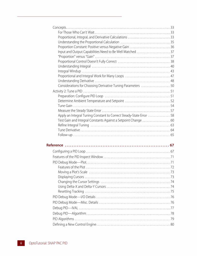
Reference . . . . . . . . . . . . . . . . . . . . . . . . . . . . . . . . . . . . . . . . . . . . . . . . . . . . . . . . . . . . . 67
Configuring a PID Loop . . . . . . . . . . . . . . . . . . . . . . . . . . . . . . . . . . . . . . . . . . . . . . . . . . . . . . . . . . 67Features of the PID Inspect Window . . . . . . . . . . . . . . . . . . . . . . . . . . . . . . . . . . . . . . . . . . . . . . 71PID Debug Mode—Plot. . . . . . . . . . . . . . . . . . . . . . . . . . . . . . . . . . . . . . . . . . . . . . . . . . . . . . . . . . 71
Features of the Plot . . . . . . . . . . . . . . . . . . . . . . . . . . . . . . . . . . . . . . . . . . . . . . . . . . . . . . . . . . 72Moving a Plot’s Scale . . . . . . . . . . . . . . . . . . . . . . . . . . . . . . . . . . . . . . . . . . . . . . . . . . . . . . . . 73Displaying Cursors . . . . . . . . . . . . . . . . . . . . . . . . . . . . . . . . . . . . . . . . . . . . . . . . . . . . . . . . . . . 73Changing the Cursor Settings . . . . . . . . . . . . . . . . . . . . . . . . . . . . . . . . . . . . . . . . . . . . . . . . 74Using Delta-X and Delta-Y Cursors . . . . . . . . . . . . . . . . . . . . . . . . . . . . . . . . . . . . . . . . . . . . 74Resetting Tracking . . . . . . . . . . . . . . . . . . . . . . . . . . . . . . . . . . . . . . . . . . . . . . . . . . . . . . . . . . . 75
PID Debug Mode—I/O Details . . . . . . . . . . . . . . . . . . . . . . . . . . . . . . . . . . . . . . . . . . . . . . . . . . . 76PID Debug Mode—Misc. Details . . . . . . . . . . . . . . . . . . . . . . . . . . . . . . . . . . . . . . . . . . . . . . . . . 76Debug PID—IVAL . . . . . . . . . . . . . . . . . . . . . . . . . . . . . . . . . . . . . . . . . . . . . . . . . . . . . . . . . . . . . . . 77Debug PID—Algorithm . . . . . . . . . . . . . . . . . . . . . . . . . . . . . . . . . . . . . . . . . . . . . . . . . . . . . . . . . . 78PID Algorithms . . . . . . . . . . . . . . . . . . . . . . . . . . . . . . . . . . . . . . . . . . . . . . . . . . . . . . . . . . . . . . . . . . 79Defining a New Control Engine . . . . . . . . . . . . . . . . . . . . . . . . . . . . . . . . . . . . . . . . . . . . . . . . . . . 80

OptoTutorial: SNAP PAC PID 11
Chapter i
1: Introduction
How to Use This TutorialThis tutorial shows how to configure and tune a PID loop on a SNAP PAC rack-mounted controller or brain, using the SNAP PAC Learning Center. The introduction describes the hardware, firmware, and software needed to complete the tutorial.
Each lesson has two sections: Concepts and Activity.
• The Concepts section provides general background information; you do not need a SNAP PAC Learning Center to benefit from this section. If you have little experience with PID or need a refresher, you’ll find the Concepts sections especially helpful.
• The Activity section provides step-by-step instructions for using PAC Control with a SNAP PAC Learning Center and is independent of the Concepts section. In other words, you do not need to study the Concepts before following the Activities.
Also, this tutorial assumes that you may at any point be eager to depart from the instructional sequence and explore the PID features. Sections entitled “For Those Who Can’t Wait” provide some guidance.
Skills You’ll Learn in this Tutorial
Lesson 1: Basic PID Control• Configuring input, output, and setpoint
• Defining valid range of input
• Clamping output
• Configuring scan interval
• Observing a PID
• Changing tuning parameters in real time
• Adjusting views of a graph: changing resolution of X and Y axes
• Determining system dead time and scan interval

WHAT YOU NEED
OptoTutorial: SNAP PAC PID2
Lesson 2: Understanding Proportional, Integral, and Derivative• Setting gain constants for heating and cooling systems
• Understanding proportional control
• Understanding the integral calculation and the I constant
• Understanding the Derivative calculation and the D constant
• Tuning a PID loop
What You NeedSkills—A basic understanding of PAC Control (provided by the SNAP PAC Learning Center User’s Guide or by the PAC Control User’s Guide).
Hardware—SNAP PAC™ Learning Center
Software—PAC Project Basic or PAC Project Pro
Configuration file—The sample PAC Control Tag database PIDPoints.otg is provided with the Learning Center or in a separate downloadable zip file (OptoTutorial 1641: PID with PAC Control). The .otg file provides the point configuration for the heater and temperature probe used in this tutorial.
SNAP PAC Learning CenterBecause this tutorial is a supplement to the SNAP PAC Learning Center, this tutorial assumes the following:
• The Learning Center is assembled according to the directions in the SNAP PAC Learning Center Guide (Opto 22 form #1638).
• Communication is established between your computer and the SNAP PAC.
The SNAP PAC Learning Center provides a combination temperature probe and heater, used in this tutorial to demonstrate PID control over a heating system.
CHAPTER 1: INTRODUCTION
OptoTutorial: SNAP PAC PID 33
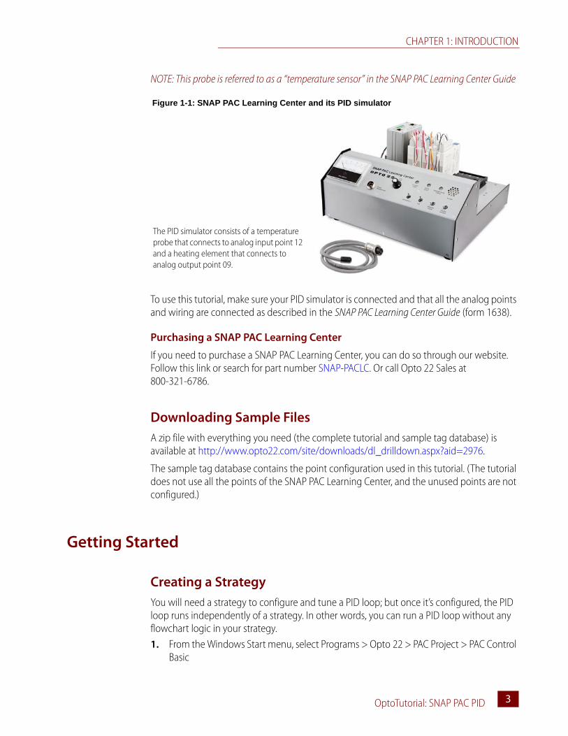
NOTE: This probe is referred to as a “temperature sensor” in the SNAP PAC Learning Center Guide
To use this tutorial, make sure your PID simulator is connected and that all the analog points and wiring are connected as described in the SNAP PAC Learning Center Guide (form 1638).
Purchasing a SNAP PAC Learning Center
If you need to purchase a SNAP PAC Learning Center, you can do so through our website. Follow this link or search for part number SNAP-PACLC. Or call Opto 22 Sales at 800-321-6786.
Downloading Sample FilesA zip file with everything you need (the complete tutorial and sample tag database) is available at http://www.opto22.com/site/downloads/dl_drilldown.aspx?aid=2976.
The sample tag database contains the point configuration used in this tutorial. (The tutorial does not use all the points of the SNAP PAC Learning Center, and the unused points are not configured.)
Getting Started
Creating a StrategyYou will need a strategy to configure and tune a PID loop; but once it’s configured, the PID loop runs independently of a strategy. In other words, you can run a PID loop without any flowchart logic in your strategy. 1. From the Windows Start menu, select Programs > Opto 22 > PAC Project > PAC Control
Basic
The PID simulator consists of a temperature probe that connects to analog input point 12 and a heating element that connects to analog output point 09.
Figure 1-1: SNAP PAC Learning Center and its PID simulator
GETTING STARTED
OptoTutorial: SNAP PAC PID4
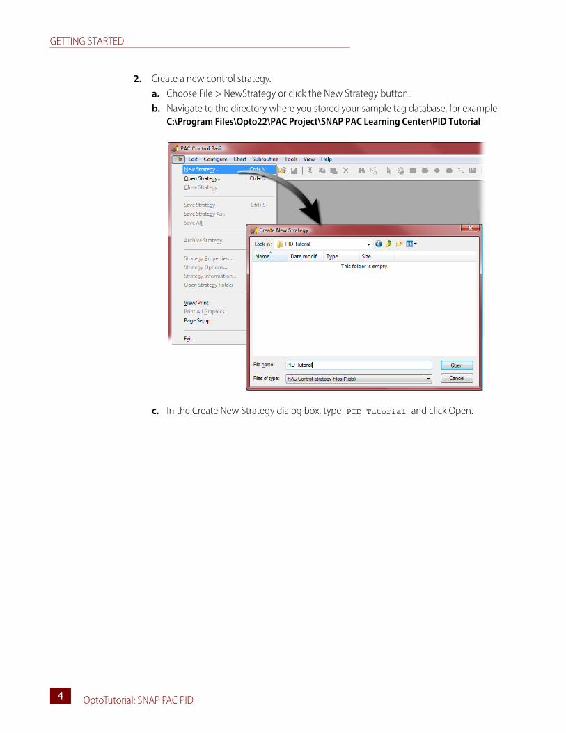
2. Create a new control strategy.a. Choose File > NewStrategy or click the New Strategy button.b. Navigate to the directory where you stored your sample tag database, for example
C:\Program Files\Opto22\PAC Project\SNAP PAC Learning Center\PID Tutorial
c. In the Create New Strategy dialog box, type PID Tutorial and click Open.

CHAPTER 1: INTRODUCTION
OptoTutorial: SNAP PAC PID 55
3. Associate your Control Engine.
4. Import the tag database.a. Right-click the I/O Units folder.b. Select Import.
a. Right-click the Control Engines folder.
b. From the pop-up menu, click Add.
c. In the Configure Control Engines dialog box, click Add.
d. The Control Engine you defined for your SNAP PAC Learning Center should be displayed in the Select Control Engine dialog box (if not, see “Defining a New Control Engine” on page 80).
e. Select your Control Engine and click OK.
f. Click OK to close the Configure Control Engines dialog box.
GETTING STARTED
OptoTutorial: SNAP PAC PID6
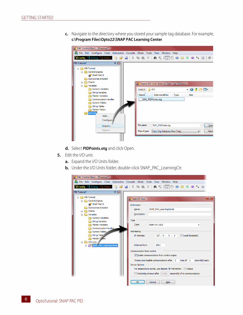
c. Navigate to the directory where you stored your sample tag database. For example, c:\Program Files\Opto22\SNAP PAC Learning Center
d. Select PIDPoints.otg and click Open.5. Edit the I/O unit.
a. Expand the I/O Units folder.b. Under the I/O Units folder, double-click SNAP_PAC_LearningCtr.

CHAPTER 1: INTRODUCTION
OptoTutorial: SNAP PAC PID 77
c. Change the IP address to the IP address of your SNAP PAC.
NOTE: Alternatively, you can use the Loopback IP address (127.0.0.1). This directs PAC Control to use the same IP address that is configured for the Control Engine. (The loopback I/O address is explained in Lesson 2 of the SNAP PAC Learning Center Guide).
Ready for the TutorialYou are ready for the activities when you have the following configured:
Control engine
Learning Center (Import configuration from PIDPoints.otg; change IP address.)
Module 02, Point 09, analog output point (controls a heating element in the PID simulator)
Module 03, Point 12, analog input point (reports the temperature of the PID simulator)
Module 04, Point 16, analog input point (connects to the Learning Center potentiometer. This lets you optionally control the setpoint with the potentiometer.)
GETTING STARTED
OptoTutorial: SNAP PAC PID8
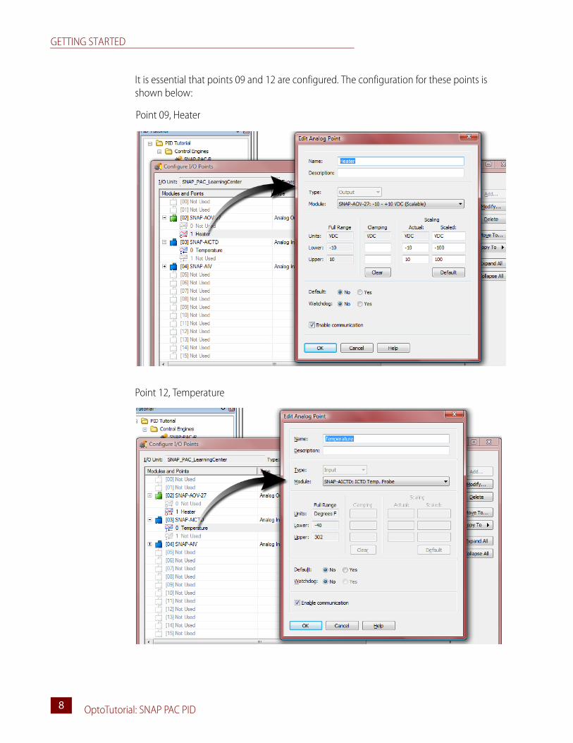
It is essential that points 09 and 12 are configured. The configuration for these points is shown below:
Point 09, Heater
Point 12, Temperature

CHAPTER 1: INTRODUCTION
OptoTutorial: SNAP PAC PID 99
For Those Who Can’t WaitThe goal of this tutorial is to present a thorough, step-by-step explanation of the concepts of PID and features provided in PAC Control. For users who prefer to experiment first, here is a summary of the features that can be configured in PAC Control.
A SNAP PAC rack-mounted controller or brain provides 96 PID loops. Each PID loop can be configured with unique settings for the following:
• Input variable (process variable)
• Setpoint
• Output (controller output)
• PID algorithm
• Constants for proportional, integral, and derivative
• PID scan time
• Feed forward gain
• Out-of-range input (upper and lower)
• Upper and lower clamps on controller output
• Minimum and maximum changes in output
• Scaling of input and output
Essential configuration for all PID loops:
• Scan rate
• Input (process variable)
• Output (controller output)
• Setpoint
• PID algorithm
• Input low and high range
• Positive or negative gain value. (For the Learning Center’s heating system, use a negative gain. For more discussion on gain, see “Proportion Constant: Positive versus Negative Gain.” on page 36.)
Optional configuration parameters:
• Output upper and lower clamps
• Output minimum change
• Output maximum change
• Output for assumed failure
• Feed forward gain
• Calculate square root of input

GETTING STARTED
OptoTutorial: SNAP PAC PID10
Once the basic configuration settings are made, the following must be done:
• The strategy must be downloaded to the SNAP PAC.
• The strategy must be run to save the PID configuration to the I/O unit.
• The Mode must be set to Auto. (Auto is the default setting.)
• Communication with PAC Control must be Enabled. (Enabled is the default setting.)

Optotutorial: SNAP PAC PID 1111
Chapter 1
2: Basic PID Control
Skills You Will LearnIn PAC Control Configure mode:
• Configuring input, output, and setpoint
• Defining valid range of input
• Clamping output
• Configuring scan interval
In PAC Control Debug mode:
• Observing a PID
• Changing tuning parameters in real time
• Adjusting views of a graph: changing resolution of X and Y axes
• Determining system dead time and scan interval
Concepts
What is PID?A proportional integral derivative (PID) control system monitors a process variable, compares the process variable to a setpoint, and calculates an output to correct any difference (error) between the setpoint and process variable. The mathematical formulas that do this vary, but all PID systems share fundamental concepts:
• They evaluate a process variable against its setpoint.
• They control an output to reduce the difference between the process variable and setpoint.
• The output is the result of proportional, integral, and derivative calculations.
• The effects of proportional, integral, and derivative calculations are modified by user-determined P, I, and D constants.

CONCEPTS
Optotutorial: SNAP PAC PID12
• The P, I, and D constants need to be adjusted (or tuned) for each system.
Where PID Resides in a SNAP PAC SystemIn the SNAP PAC system, the PID algorithm runs independently of PAC Control, so the PAC Control strategy doesn’t need to monitor every variable and configuration setting associated with the PID algorithm.
In the SNAP PAC R, both PAC Control and PID run on the same hardware, but the two parts remain independent.
PAC Control can change configuration settings and start and stop PIDs.
PID loops run independently of PAC Control.

CHAPTER 2: BASIC PID CONTROL
Optotutorial: SNAP PAC PID 1313
A Simple PID SystemA tank, thermostat, and heater is a system with all the elements required for PID control:
In this tank heating system, the process variable (PV) is the temperature of the tank. The setpoint is supplied by a thermostat. The controller compares the setpoint to the process variable and decides the appropriate output to achieve the setpoint. But the system becomes complex because of the following:
• The output of the PID loop must be scaled to the output device. For example, to turn up the heat, the controller must convert a difference in temperature to a setting on a gas valve controlling a heater. Increasing the temperature by 10 degrees may mean opening the gas valve by 10%, 5%, or 50%—this varies according to the device.
• The difference between the setpoint and the process variable is called the error. This error is changing in time, so the controller output must also be changing to avoid overshooting the setpoint.
• A PID algorithm not only maintains a process variable at a setpoint; it must also react to disturbances, which are external factors affecting the stability of the system. Typical disturbances are a change in load (for example, filling the tank) or a change in setpoint.
• Equipment and safety limitations may restrict how quickly you can change a setting in the output device or what conditions determine when the output device can be turned on or off.
• The range of valid input for the process variable should be defined so the PID can properly react to or ignore out-of-range inputs.
Figure 2-1: A Basic PID System
Temperature is the process variable monitored by the PID loop used with this tutorial. The process variable is also referred to as the PID input, or just input. The PID’s output is used to control a device that will have an effect on the process variable, in this case a heater. A PID loop’s output is often referred to as the “Controller Output.” In this context, the controller output is referring to the PID and not to PAC Control’s control engine.
The examples throughout will use sample values comparable to what you would get with the PID simulator probe (supplied with the SNAP PAC Learning Center) at room temperature. Controlling temperature is one type of PID system. Others may control pressure, mixture ratios, cooling, flow rate, and so on.
Process Variable (PV)Temperature Controller
Setpoint
A thermostat provides the desired setting for tank temperature
Output DeviceHeat Source
ControllerOutput
PV = 70
PV should be: 80
Heater output should be increased/ decreased

CONCEPTS
Optotutorial: SNAP PAC PID14
The diagram below shows more elements of this system.
Figure 2-2: Details of a Basic PID System
NOTE: PAC Control calculates error by subtracting the Setpoint from the Process Variable. This calculation creates a negative error when the Process Variable is below the setpoint. This mode is used for “pump-up” control, such as maintaining level, pressure, flow, and heating.
Process Variable (PV):Tank temperature, reported by temperature sensor
Output Variable:Percentage that gas valve is open, which in turn controls the heater
Controller Output
Other factors in calculation of controller output are not shown, such as scaling of the output variable, clamps to its range, and minimum or maximum on and off times.
The error is the basis of the controller output. The PID controller manipulates this variable with proportional, integral, and derivative calculations.
Use Error to Calculate Controller Output
Setpoint may be a setting within the PID controller, read from an instrument or operator interface, or the output from another PID loop.
80 degrees
Setpoint
PID Controller
Calculate Error:(Error = Process Variable – Setpoint)
70° F
Heat
70
80
10
Input to PID
Output to heater

CHAPTER 2: BASIC PID CONTROL
Optotutorial: SNAP PAC PID 1515
Plotting the Simple SystemIn this tank heating system, the process variable and setpoint are on the same scale, while the controller output is on a different scale. If the values of the process variable, setpoint, and output are plotted in time, they would form the graphs shown below.
In these graphs, the Y-axis represents the values of the process variable, setpoint, and controller output. The X-axis represents time. The X-axis is shown with demarcations for units of time. Though the process variable is changing continuously, the controller only knows its value when the process variable is scanned. The vertical lines represent the scan interval, which is an important component in configuring a PID loop.
Figure 2-3: Plots of the Process Variable, Setpoint, and Output
Process Variable and Setpoint
Controller output corrects and stabilizes systemStable system
System disturbance, e.g., tank is filled
Process variable restored to setpoint
Output Variable
Gas valve 80% open
Setpoint
Process Variable
Gas valve 20% open
Output
Time
Time
150° F
0° F
100%
0%

CONCEPTS
Optotutorial: SNAP PAC PID16
The chart below shows the step changes in controller output.
Figure 2-4 shows how the configured scan interval affects the controller output. With shorter scan intervals, the output graph resembles a continuous curve, with frequent controller adjustment and therefore better control of the process variable. Setting an appropriate scan interval is critical to successful PID tuning.
To summarize, Figures 2-1 through 2-4 show the following concepts relevant to PID configuration and tuning:
• Setpoint, process variable, output, and scan interval are the key components of the system.
• Setpoint can be from an input device or any variable accessible to the controller.
• The output device can be a physical device that effects change, or it can be used as the input or setpoint to another PID. In this example, the output controls a heater.
• The setpoint and process variable are on the same scale.
• The output device (heater) may be on the same scale as the process variable and the setpoint, but often it is not.
Figure 2-4: Actual Values of Process Variable, Setpoint, and Output over Time
NOTE: The input change is truly continuous, as it is shown here. The output, however, is a step shape. At each scan, the controller sets an output value that continues unchanged until the next scan.
Process Variable, Setpoint, and Controller Output
Error at time of scan
Setpoint
Process Variable (Input)
Time
Controller output at time of scanOutput (Correction)
TimeScan interval
CHAPTER 2: BASIC PID CONTROL
Optotutorial: SNAP PAC PID 1717
• Scan interval is the interval at which the controller evaluates the process variable against the setpoint and calculates the output.
System Dead Time and Scan Interval (Scan Rate)All PID calculations occur at a time interval you specify by choosing a scan rate when you configure the PID. This makes scan rate a very important setting. The value you use for scan rate will vary with each system, and measuring the system dead time can help you assess the value of your scan interval.
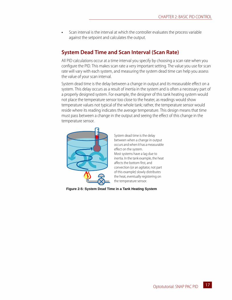
System dead time is the delay between a change in output and its measurable effect on a system. This delay occurs as a result of inertia in the system and is often a necessary part of a properly designed system. For example, the designer of this tank heating system would not place the temperature sensor too close to the heater, as readings would show temperature values not typical of the whole tank; rather, the temperature sensor would reside where its reading indicates the average temperature. This design means that time must pass between a change in the output and seeing the effect of this change in the temperature sensor.
System dead time is the delay between when a change in output occurs and when it has a measurable effect on the system.Most systems have a lag due to inertia. In the tank example, the heat affects the bottom first, and convection (or an agitator, not part of this example) slowly distributes the heat, eventually registering on the temperature sensor.
Figure 2-5: System Dead Time in a Tank Heating System
CONCEPTS
Optotutorial: SNAP PAC PID18
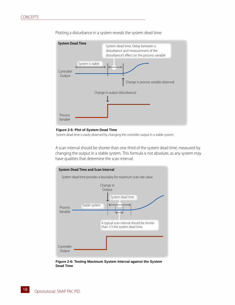
Plotting a disturbance in a system reveals the system dead time:
A scan interval should be shorter than one-third of the system dead time, measured by changing the output in a stable system. This formula is not absolute, as any system may have qualities that determine the scan interval.
Figure 2-5: Plot of System Dead Time
System dead time is easily observed by changing the controller output in a stable system.
System Dead Time
Change in output (disturbance)
Change in process variable observed
System dead time: Delay between a disturbance and measurement of the disturbance’s effect on the process variable
Controller Output
Process Variable
System is stable
Figure 2-6: Testing Maximum System Interval against the System Dead Time
System Dead Time and Scan Interval
System dead time provides a boundary for maximum scan rate value.
Controller Output
Process Variable
Change in Output
Stable system
System dead time
A typical scan interval should be shorter than 1/3 the system dead time.

CHAPTER 2: BASIC PID CONTROL
Optotutorial: SNAP PAC PID 1919
For example, equipment limitations may require longer intervals. In many systems, however, the scan interval is faster than the time required to observe a change in the process variable, which can cause the controller to overcorrect. Any overcorrection can be removed with proper tuning of the PID, which is explained in Lesson 2.
In Activity 1, you will configure a PID loop controlling a heating system and observe the lag in this system. This activity will provide practice with using the PID in manual mode and with manipulating its plot.
Activity 1: Configure System and Observe System Dead Time
Preparation1. Start PAC Control.2. Open your strategy.
Configure PIDYou will configure only the basic components needed to observe system dead time. Configuring additional features may interfere with determining the system dead time. For example, you do not want your PID loop to exercise any control, so you will want to be in Manual mode. Rather, you just want to plot the input (process variable), setpoint, and output (controller output).1. Select Mode > Configure.2. Open PID Loop configuration.
a. In the strategy tree, right-click the PIDs folder.
ACTIVITY 1: CONFIGURE SYSTEM AND OBSERVE SYSTEM DEAD TIME
Optotutorial: SNAP PAC PID20
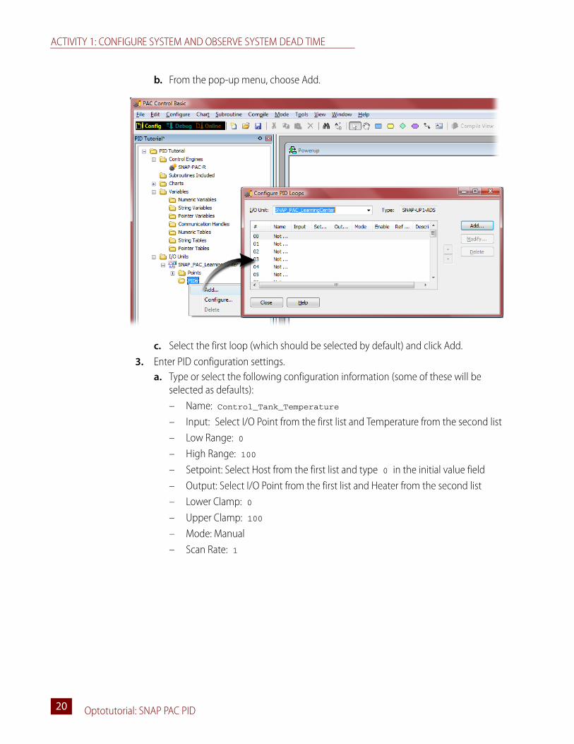
b. From the pop-up menu, choose Add.
c. Select the first loop (which should be selected by default) and click Add.3. Enter PID configuration settings.
a. Type or select the following configuration information (some of these will be selected as defaults):– Name: Control_Tank_Temperature– Input: Select I/O Point from the first list and Temperature from the second list– Low Range: 0– High Range: 100– Setpoint: Select Host from the first list and type 0 in the initial value field– Output: Select I/O Point from the first list and Heater from the second list– Lower Clamp: 0– Upper Clamp: 100– Mode: Manual– Scan Rate: 1

CHAPTER 2: BASIC PID CONTROL
Optotutorial: SNAP PAC PID 2121
b. Click OK to close the Add PID Loop dialog box.c. Click Close to close the Configure PID Loop dialog box.
Notice that your PID loop is now listed under the PIDs folder:
Name your PID loop.
Select point used as the process variable.
Low and high range: define valid input
Setpoint: Host allows you to control setpoint from PAC Control
The heater is scaled to percent, so 0 and 100 prevent the PID from
calculating outputs that are outside of this logical range.
Mode: Manual prevents the PID from making output changes so you observe
the system dead time.
Scan rate: Use 1 as a starting point. This number determines how often the input is scanned and the controller
output is updated.
Select point used as output device.

ACTIVITY 1: CONFIGURE SYSTEM AND OBSERVE SYSTEM DEAD TIME
Optotutorial: SNAP PAC PID22
Determine Scan Interval1. Download and run the strategy.
a. Choose Configure > Debug.b. Acknowledge any download messages.c. When in Debug mode, choose Debug > Run.
Running the strategy sends the PID configuration to the I/O configuration.
2. Open the PID viewer.
Control Engine and I/O Unit
Control EngineThe control engine is the brain's onboard capability for controlling one or more I/O units using a PAC Control strategy.
I/O UnitThe I/O unit is the part of the brain devoted to management of the I/O modules. This part can be configured in PAC Control or in PAC Manager (and then imported into PAC Control).
The I/O unit configuration imported or created in PAC Control is loaded to the I/O unit when the strategy is run.
Debug Run
Control logic
I/O unit configuration
Flowcharts and variables
Active I/O unit configuration

CHAPTER 2: BASIC PID CONTROL
Optotutorial: SNAP PAC PID 2323
3. In the PIDs folder, double-click Control_Tank_Temperature.
Your PID should be operating as follows:
– Your PID is in Manual mode, so it reads the input and setpoint but makes no changes to the output.
– Your output is 0 (blue line).
– Your setpoint is 0 (yellow line).
– Your input (red line) shows the room temperature in Fahrenheit.
– Graphs for input, output, and setpoint are being plotted against time.4. Set PID output to 30 percent.
a. In the Output field, type 30.b. Click Apply.

ACTIVITY 1: CONFIGURE SYSTEM AND OBSERVE SYSTEM DEAD TIME
Optotutorial: SNAP PAC PID24
Notice change in both the PID Input and PID Output graphs.
It takes a few minutes for your system to stabilize. Viewing the input graph at a finer resolution helps you know when the system has stabilized.
Gaps in a plot indicate that scanning was interrupted, in this case, when the Output field was edited.
Enter new value for Output here and click Apply.

CHAPTER 2: BASIC PID CONTROL
Optotutorial: SNAP PAC PID 2525
5. Change view of input axis.a. Click and drag the input axis so that the plot of the input is at the bottom of the
graph:
Click and drag the input axis so that the input plot is at the bottom of the visible graph. This point will be centered when you change the input axis.
Click here to drag the axis up or down.

ACTIVITY 1: CONFIGURE SYSTEM AND OBSERVE SYSTEM DEAD TIME
Optotutorial: SNAP PAC PID26
b. Click Input Axis and select View 1% Span.

CHAPTER 2: BASIC PID CONTROL
Optotutorial: SNAP PAC PID 2727
6. Change the time axis.a. Click Time Axis and select View 1 Minute Span.
b. If your graph has stopped tracking, which can happen when focus is on any of the tuning fields, choose Reset Scale Tracking from the Time Axis menu (or click the graph).
Until you are familiar with the PID plot, it is recommended that you avoid using the shortest settings (10 seconds or 1 second) for the time axis. After you’ve observed a change in the input, you can zoom in on the graph, which is described later.

ACTIVITY 1: CONFIGURE SYSTEM AND OBSERVE SYSTEM DEAD TIME
Optotutorial: SNAP PAC PID28
7. Wait for the system to stabilize.
A stable system will exhibit little change in the input value, which is shown numerically and graphically.
Note: If your temperature doesn’t stabilize, a likely cause is a varying room temperature. Make sure your PID simulator probe is not too near to a heating or cooling outlet.
Observe the graph of the input field. The system is stable when the input value does not vary significantly (some drift in the input value can be expected). Stabilization may take several minutes, depending on the type of system.
8. Under the Time Axis menu, choose Reset.a. Click the Time Axis button.b. Click Reset Scale Tracking.
This is a precautionary step, as changing settings on the plot can cause the trend to stop plotting data. Resetting the time axis ensures that you are viewing the real-time values.
NOTE: Be prepared to do the following step quickly. In Step 9 you change the output. A change in the input will occur within a couple of seconds. As soon as you see a change in input, you will click and drag the time axis (X-Axis), which will stop the plot so you can closely examine the system dead time.
9. Observe system dead time with a 20 percent increase in output.a. Type 50 in the Output field.b. Click Apply.

CHAPTER 2: BASIC PID CONTROL
Optotutorial: SNAP PAC PID 2929
A change in the input will occur quickly:
c. Click and drag the Time Axis (X-Axis) so that the plot shows the change in output and the change in input.
10. Display a Delta X cursor.a. From the Data menu, select Cursor.
b. Right-click the cursor and choose Style > Delta X.
The input axis (upper white arrow added to this picture) begins to respond to the change in output (lower white arrow).

ACTIVITY 1: CONFIGURE SYSTEM AND OBSERVE SYSTEM DEAD TIME
Optotutorial: SNAP PAC PID30
The Delta X cursor displays the time difference between the two vertical bars.
11. Measure the System Dead Time.
The time between the change in output and the change in input represents the system dead time.
a. To set the vertical measurement bars, click a vertical line and drag it left or right. b. Place the first bar after the output change. Place the second bar before the change
in input.

CHAPTER 2: BASIC PID CONTROL
Optotutorial: SNAP PAC PID 3131
In this example, the system dead time was shown to be about 1.8 seconds. Your results may vary, but a typical system dead time for the PID simulator is around 2 seconds, suggesting that 1 second is too long of a scan interval, but 0.4 should be adequate.
12. Type a new system interval.a. In the Scan Rate field, type 0.4b. Click Apply.
13. Save Tuning.
14. Return to Configure mode.a. Click Close to close the View PID Loop (Scanning) dialog box. b. Choose Mode > Configure.
For Those Who Can’t WaitAt this point you may be very eager to complete the essential PID configuration and see a working PID.
Lesson 2 discusses gain, integral, and derivative settings. In that activity, you will observe and tune a working PID loop. All of this follows a thorough discussion of P, I, and D calculations along with an explanation of the different PID algorithms available.
If you wish to experiment on your own now and see your PID loop, you will need to change the settings as described below.
NOTE: With a scan interval of 1 second you may conclude that your measurement of the system dead time is accurate to the nearest second. However, the PID viewer plots the current values of the Process Variable and Setpoint, regardless of the scan time. Therefore, your measurement of system dead time is accurate.
In most applications, you can set the scan rate as fast as possible and use this test of system dead time only to better understand the reaction time of your system. The SNAP PAC will easily handle shorter scan intervals, and for many applications you might begin tuning by setting the scan rate to 0.1.
a. Click the Save Tuning button.
b. Click Yes.

ACTIVITY 1: CONFIGURE SYSTEM AND OBSERVE SYSTEM DEAD TIME
Optotutorial: SNAP PAC PID32
1. In Configure mode, open the PID loop configuration.a. In the Strategy Tree, right-click PID ControlTankTemperature.b. Select Modify.
2. Type or select the following configuration information.
3. Download your strategy.4. Start your strategy.5. Open the PID Inspect dialog box.
It is recommended that you observe your loop’s response to setpoint changes a few degrees above room temperature.
When finished, return to Configure mode.
a. Setpoint: Change from Host to I/O Point – Setpoint.This setting will get the setpoint from the potentiometer.
b. Mode: Change Manual to Auto.
c. Gain: Change 1 to –10
In lesson 2, you will see why it is critical for this system to have a negative number for the gain constant.
d. Integral: Change 0 to 0.5
OptoTutorial: SNAP PAC PID 3333
Chapter 2
3: Understanding Proportional, Integral, and Derivative
Skills You Will Learn• Setting gain constants for heating and cooling systems
• Understanding proportional control
• Understanding the integral calculation and the I constant
• Understanding the derivative calculation and the D constant
• Tuning a PID loop
Concepts
For Those Who Can’t WaitThis lesson provides a thorough discussion of proportion, integral, and derivative calculations as they are deployed in PAC Control’s algorithms. Though the Concepts section provides useful background to Activity 2, you may wish to begin the activity after reading the concepts on proportional control and then resume reading the Concepts section when the Activity begins to tune the integral.
Proportional, Integral, and Derivative CalculationsWe intuitively use PID when making corrections to driving, cooking, walking, and so on. The trick is getting machinery to do what humans do: examine the system, apply corrective input, watch, compensate, and anticipate.
A PID algorithm is designed to do this with numbers. It calculates a difference between the current and desired values and uses this difference, called error, to apply a corrective response. The error is examined over time with the help of the integral term, which corrects any tendency of the system to stabilize at the wrong value. The rate of change is analyzed by the derivative calculation, which tries to dampen a tendency to overcorrect.

CONCEPTS
OptoTutorial: SNAP PAC PID34
A successful PID loop requires well-chosen constants for gain, integral, and sometimes derivative (many loops work with P and I constants only). Choosing your constants is part understanding their role in the PID algorithm (explained in this tutorial) and part trial and error, a process referred to as tuning.
The SNAP PAC offers five PID algorithms:
• Velocity Type B (the default type)
• Velocity - Type C (available only for PAC-R, EB, and SB with firmware version 8.5e and higher)
• ISA
• Parallel
• Interacting
The offering of five algorithms illustrates that there is no one formula for PID control. Each algorithm has unique qualities, but the general concepts of proportional, integral, and derivative, and tuning constants, is similar across all. The following discussion describes generalizations of the effect of P, I and D components of the calculation. Specific attributes of the calculation will be explained as well.
Figure 3-7: Heating System with Gain, Integral, and Derivative
The PID algorithm uses the process variable and setpoint to make gain, integral, and derivative calculations. These separate calculations are referred to as the Proportional Term, Integral Term, and Derivative Term. Each of these terms reacts to error or error over time. The extent to which each term influences the controller output is determined by the P, I, and D tuning constants.
Process Variable (PV)
(Input)
PID Controller
Output Device
Controller Output
Controller output comprises proportional, integral, and derivative calculations. The influence of each part of the calculation depends in part on the values you assign to constants during a process called tuning.
Calculate Error
Setpoint
Heat
Proportional Term
Integral Term
Derivative Term
Output

CHAPTER 3: UNDERSTANDING PROPORTIONAL, INTEGRAL, AND DERIVATIVE
OptoTutorial: SNAP PAC PID 3535
Understanding the Proportional CalculationIn proportional control, the output signal is a proportional response to the error signal. This proportional response is achieved by the gain constant.
Figure 3-8 shows proportional control as a teeter-totter, where the size of the error has a direct effect on the controller output.
Figure 3-8: Proportional Control
Proportional Control
Error signal(Deviation from
setpoint) Output response (heater)
In proportional control, the output signal is a proportional (or multiplied) response to the error signal. Here is shown a gain of 1. Moving the blue triangle left or right is analogous to using a higher or lower gain setting.
Setpoint
Temperature (Input)
Figure 3-9: Effect of Various Gain Settings
Imagine the black line swinging up or down depending on the value of the process variable. With a gain of 1, the error and controller output are equal.
In this analogy, increasing the gain moves the fulcrum point (the triangle ) left, where a small error can produce a large change in the controller output. Decreasing the gain moves the fulcrum point to the right, where the error produces less change in controller output.
All of these gain settings are examples of proportional responses to the error.
Gain in Proportional Control
Setpoint
Setpoint
Setpoint
Error
Error
Controller output
Controller output
Controller output
Gain > 1
Gain =1
0 < Gain < 1

CONCEPTS
OptoTutorial: SNAP PAC PID36
Proportion Constant: Positive versus Negative GainThe gain constant used in the PID algorithms can be a positive or negative number. When the process variable drops below setpoint in a heating system, the error is a negative number. This negative number must be converted to a positive number that increases the heater’s output. Using a negative gain constant achieves this. The reverse is required for cooling: exceeding the setpoint should result in a controller output that increases the output of a cooling device. Figure 3-10 compares the effects of positive and negative gain constants in heating and cooling systems.
Figure 3-10: Heating and Cooling, Positive and Negative Gain
Proportional Control: Positive and Negative P Constants
A proportional response to the error is achievedby multiplying the error by a constant.
P constant can be positive, negative, whole number, or fraction.
Heating System and Negative P Constant
Cooling System and Positive P Constant
When using proportional control in a heating system, a negative constant achieves the desired controller output.
When using proportional control in a cooling system, a positive constant achieves the desired controller output.
Setpoint
Input: Temperature
Output response (Heater)
Output response
(Fan)
Setpoint
Input: Temperature
E = ErrorP = Proportion constant
CO = Controller output
CHAPTER 3: UNDERSTANDING PROPORTIONAL, INTEGRAL, AND DERIVATIVE
OptoTutorial: SNAP PAC PID 3737
Input and Output Capabilities Need to Be Well MatchedThere are several layers of design that achieve the appropriate balance between the output device and the process variable being controlled:
• The physical equipment—In the tank example, the heater must have the capacity to change the tank temperature within the time required by the application.
• The selection and scaling of the module—All PID calculations reduce to ranges that the input and output modules are capable of attaining. If you have an output device that responds to values of 0 to 10 volts, then a module of this range offers the best resolution.
• The valid range options in PID configuration—One of the uses of these ranges is to calculate a value called span, which is used in all the PID algorithms provided in PAC Control. Span is a ratio of the output range to the input range and has the effect of correlating the input and output scales.
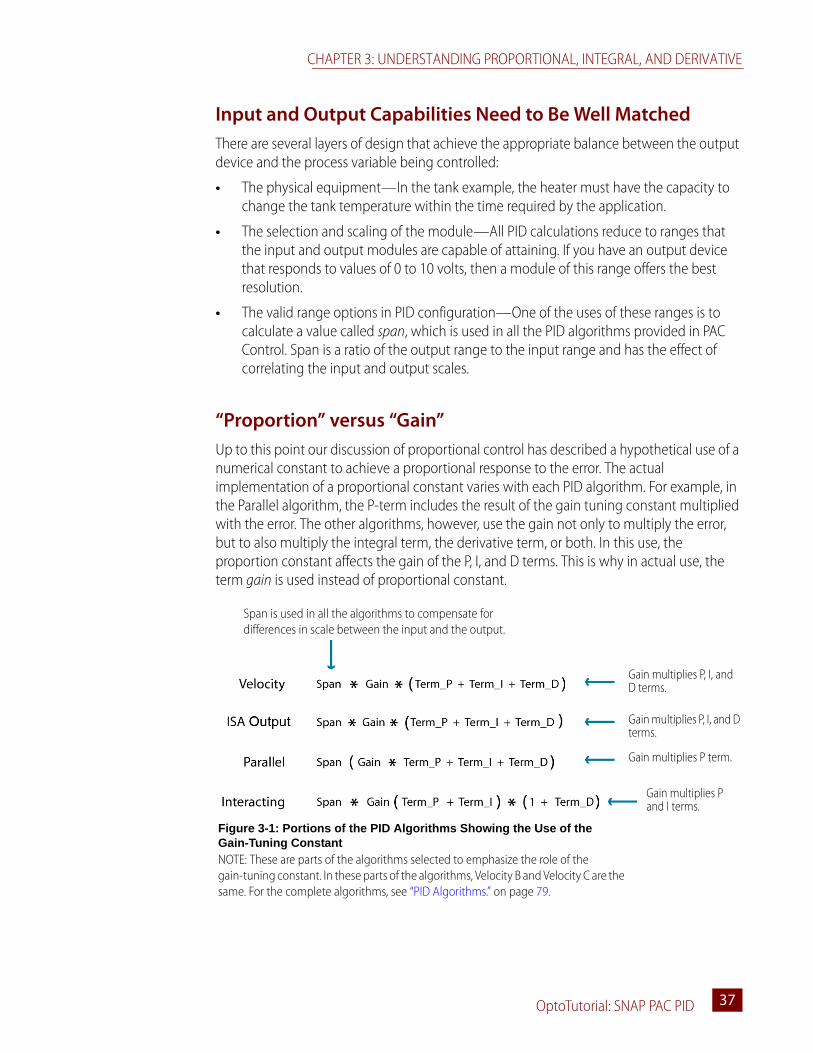
“Proportion” versus “Gain”Up to this point our discussion of proportional control has described a hypothetical use of a numerical constant to achieve a proportional response to the error. The actual implementation of a proportional constant varies with each PID algorithm. For example, in the Parallel algorithm, the P-term includes the result of the gain tuning constant multiplied with the error. The other algorithms, however, use the gain not only to multiply the error, but to also multiply the integral term, the derivative term, or both. In this use, the proportion constant affects the gain of the P, I, and D terms. This is why in actual use, the term gain is used instead of proportional constant.
Span is used in all the algorithms to compensate for differences in scale between the input and the output.
Gain multiplies P, I, and D terms.
Gain multiplies P, I, and D terms.
Figure 3-1: Portions of the PID Algorithms Showing the Use of the Gain-Tuning Constant
NOTE: These are parts of the algorithms selected to emphasize the role of the gain-tuning constant. In these parts of the algorithms, Velocity B and Velocity C are the same. For the complete algorithms, see “PID Algorithms.” on page 79.
Gain multiplies P term.
Gain multiplies P and I terms.

CONCEPTS
OptoTutorial: SNAP PAC PID38
Proportional Control Doesn’t Fully CorrectThere are many control devices that use gain only. For example, a float on a tank valve can be used to control the opening of an intake valve. As the float rises, it slowly closes the valve. In this mechanical control system, where there is no change in setpoint, a proportional correction can be adequate. However, most systems that use PID control will not be adequately controlled using a proportional correction only. For example:
• Some systems will overshoot the setpoint, creating an undesirable oscillation between overcorrection and undercorrection. Such a system is unstable, inadequate for changing load or setpoint, and may cause excessive wear on the equipment.
• In systems where a proportional correction is stable, the process variable often stabilizes at the wrong value. This is called steady-state error or offset. To correct for this, you need to look at error over time.
Figure 3-11 depicts the proportional-only correction in one system with an arbitrary gain constant of –2, chosen to keep the arithmetic simple. The tank is exposed to a 50° F breeze.
In calculation 1 (see in Figure 3-11), a 50° F input (process variable) generates an error of –20, which is multiplied by –2 to create a controller output of 40. All of the controller output goes toward raising the process variable to the setpoint.
In calculation 2 ( ), the tank temperature has been raised to 55° F, so the error is –15. This generates a controller output of 30. However, as the tank is now above the ambient temperature, part of the energy intended to correct the error is being used to compensate for heat lost to the environment.
As the process variable continues to rise ( and ), the output decreases while more of its energy is used to maintain against heat loss and less goes to raising the temperature to the setpoint. Eventually, all of the controller output goes to just maintaining the tank against heat loss.
In this example, an error of -5 maintains the temperature at 65 degrees, which in turn produces a controller output of 10. The output of 10 produces an error of –5, which perpetuates the current state.
1
2
3 4

CHAPTER 3: UNDERSTANDING PROPORTIONAL, INTEGRAL, AND DERIVATIVE
OptoTutorial: SNAP PAC PID 3939
So in this example, the controller output matches the heat needed to maintain the temperature's current status. There is no guarantee that this equilibrium occurs at the setpoint. If it did, it would do so for one load, one setpoint, and one gain setting. If setpoint, load, or both change, an offset would still occur.
Figure 3-11: Proportional Control and Steady State Error
This is a simplified example of what can happen in a system with one gain constant. The top of the gray box restates how the error is calculated. A gain constant of –2 is arbitrarily chosen to keep the arithmetic simple. The circled numbers (1–4) show the controller calculations at different values for the process variable. The hatched ( ) and solid ( )bars in the controller output box show how much of the controller output is used to correct the error.
Proportional-only control usually has a steady-state error, also called offset.
Cool breeze50° F
Process variableSetpoint
Error Setpoint = 70
If process variable is: Error is: Controller output is:
Heat
65 –5 –2 10
60 –10 –2 20
55 –15 –2 30
50 –20 –2 40
Energy required to maintain temperature against heat loss.
Controller output used to raise temperature.
CONCEPTS
OptoTutorial: SNAP PAC PID40
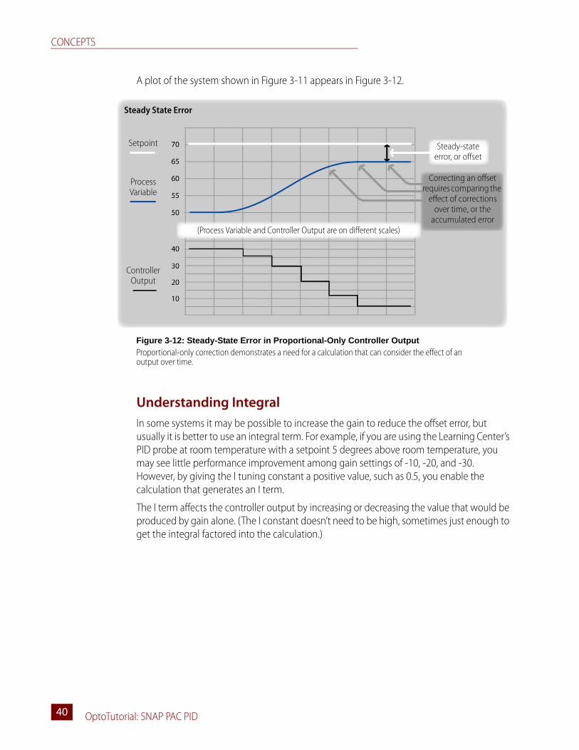
A plot of the system shown in Figure 3-11 appears in Figure 3-12.
Understanding IntegralIn some systems it may be possible to increase the gain to reduce the offset error, but usually it is better to use an integral term. For example, if you are using the Learning Center’s PID probe at room temperature with a setpoint 5 degrees above room temperature, you may see little performance improvement among gain settings of -10, -20, and -30. However, by giving the I tuning constant a positive value, such as 0.5, you enable the calculation that generates an I term.
The I term affects the controller output by increasing or decreasing the value that would be produced by gain alone. (The I constant doesn’t need to be high, sometimes just enough to get the integral factored into the calculation.)
Figure 3-12: Steady-State Error in Proportional-Only Controller Output
Proportional-only correction demonstrates a need for a calculation that can consider the effect of an output over time.
Steady State Error
Setpoint
Process Variable
Controller Output
Correcting an offset requires comparing the
effect of corrections over time, or the
accumulated error
Steady-state error, or offset
(Process Variable and Controller Output are on different scales)

CHAPTER 3: UNDERSTANDING PROPORTIONAL, INTEGRAL, AND DERIVATIVE
OptoTutorial: SNAP PAC PID 4141
Generally, the I term modifies the controller output as shown in Figure 3-13.
Comparing a proportional calculation to an integral calculation reveals the measurement of integral to be more complicated mathematically. Proportional correction is multiplication of the error by a gain. Integral correction, however, requires the measurement of error over time.
Figure 3-13: Integral Correcting Steady-State Error
The I Term examines the cumulative error and either increases the controller output or decreases it, depending on whether the error is positive or negative. The influence of the P term will vary according to the value of the integral tuning constant.
Integral Calculation Correcting Steady-State Error
Setpoint
Process Variable
Controller Output
Correcting an offset requires comparing the
effect of two corrections over time
Steady-state error, or offset
(Process Variable and Controller Output are on different scales)
Output if P acted alone
Cumulative error at time of scan
CONCEPTS
OptoTutorial: SNAP PAC PID42
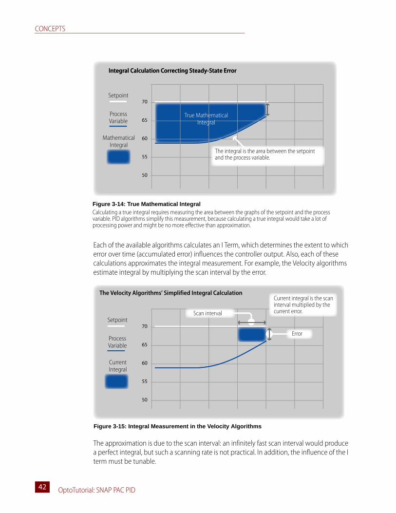
Each of the available algorithms calculates an I Term, which determines the extent to which error over time (accumulated error) influences the controller output. Also, each of these calculations approximates the integral measurement. For example, the Velocity algorithms estimate integral by multiplying the scan interval by the error.
The approximation is due to the scan interval: an infinitely fast scan interval would produce a perfect integral, but such a scanning rate is not practical. In addition, the influence of the I term must be tunable.
Figure 3-14: True Mathematical Integral
Calculating a true integral requires measuring the area between the graphs of the setpoint and the process variable. PID algorithms simplify this measurement, because calculating a true integral would take a lot of processing power and might be no more effective than approximation.
Integral Calculation Correcting Steady-State Error
Setpoint
Process Variable
The integral is the area between the setpoint and the process variable.
Mathematical Integral
True Mathematical Integral
Integral Calculation Correcting Steady-State Error
Figure 3-15: Integral Measurement in the Velocity Algorithms
Setpoint
Process Variable
Current integral is the scan interval multiplied by the current error.
Current Integral
The Velocity Algorithms’ Simplified Integral Calculation
Scan interval
Error

CHAPTER 3: UNDERSTANDING PROPORTIONAL, INTEGRAL, AND DERIVATIVE
OptoTutorial: SNAP PAC PID 4343
The influence of the I Term in the Velocity B and C algorithms is calculated with this equation:
Term I = Tune I * System Interval * Err.
Term I is 0 until a positive Tune I constant is provided. (NOTE: Tune I must be a positive number.)
The Interacting, ISA, and Parallel algorithms estimate integral by measuring the accumulated error from the current and previous scans.
The influence of the I term in the Interacting, ISA, and Parallel algorithms is calculated in these two equations: Integral = Integral + Error Term I = Tune I * System Interval * Integral
Term I is 0 until a Tune I constant is provided. Tune I must be a positive number.
With typical scan rates of 0.1 seconds, none of these algorithms measures the true mathematical integral. Nor do they need to, because the Tune I constant determines how effective Term I is in the particular application. This setting is not determined mathematically, but empirically, by watching the effect of various settings in your PID system.
Integral WindupThe Integral component of a PID calculation looks at the error over time. This allows the Integral to efficiently correct for offset. However, there are times when the cumulative error is not relevant to the necessary controller output. In our tank-heating scenario, imagine that
Figure 3-16: Integral Measurement in the ISA, Interacting, and Parallel Algorithms
Setpoint
Process Variable
Integral = 0 + 10 = 10
Current Integral
Integral Measurement in the Interacting, ISA, and Parallel Algorithms
Integral = 10 + 10 = 20
Integral = 20 + 9 = 29
Integral = 29 + 7 = 36
Integral = 36 + 3 = 38
Error

CONCEPTS
OptoTutorial: SNAP PAC PID44
the heater failed overnight and was not repaired until the following morning. After the repair, the heater runs at 100 percent for a significant length of time. Adding the error accumulated during the night makes no difference to the output —it’s still at 100 percent with or without the integral.
Integral windup refers to an integral measurement that exceeds a practical limit within the PID calculation. Typically, anytime the controller output exceeds the range of the output device, the accumulated error is irrelevant or impairs effective control when the system returns to normal.
Figure 3-17: Integral Windup
Setpoint
Process Variable
Current Integral
Integral Windup
The historical error at this point has no beneficial contribution to a controller output that is already at maximum.
Controller Output
When the system returns to normal, the historical error is irrelevant and should be discarded.
Integral accumulated error

CHAPTER 3: UNDERSTANDING PROPORTIONAL, INTEGRAL, AND DERIVATIVE
OptoTutorial: SNAP PAC PID 4545
The Velocity algorithms measure integral by multiplying the current error by the scan interval. Because this calculation only considers the current error, the Velocity algorithms do not suffer from integral windup.
In the ISA, Interacting, and Parallel algorithms, the integral measurement is an accumulation of error. These algorithms have an override function, called anti-integral windup, that is invoked when the controller output exceeds the range of the output device. (The range of the output device is set by the PID configuration settings Input–Low Range and Input–High Range.) The anti-integral windup feature does the following:
• Disables the derivative calculation (if the D tuning constant is not 0) while the output is out of range.
• Recalculates an integral value to moderate change in output when control is restored to the PID algorithm. This creates a soft landing; in contrast, the true integral or a zero integral may cause an abrupt change.
• Maintains a designated output setting (if configured to do so in the output options for when input is out of range).
• Monitors the process variable in order to relinquish control to the PID algorithm when the process variable has returned to the valid range.
Figure 3-18: Velocity Algorithms and Integral Windup
Setpoint
Process Variable
Current Integral
The Velocity Algorithms’ Simplified Integral Calculation Current integral is the scaninterval multiplied by thecurrent error.
Previous integralcalculations aren't considered in thecurrent calculation
Scan interval
Error

CONCEPTS
OptoTutorial: SNAP PAC PID46
When anti-integral windup is in effect for the ISA, Parallel, and Interacting algorithms, you are not able to see the regular PID calculations until the output returns within the range and control is restored to the algorithm.
Figure 3-19: PAC Control Debug, PID Loop Viewer
Anti-integral windup is activated in this PID heating loop in which the setpoint was lowered below the process variable. Anti-integral windup asserts control when the controller output is either over or under the range of the output device.
CHAPTER 3: UNDERSTANDING PROPORTIONAL, INTEGRAL, AND DERIVATIVE
OptoTutorial: SNAP PAC PID 4747
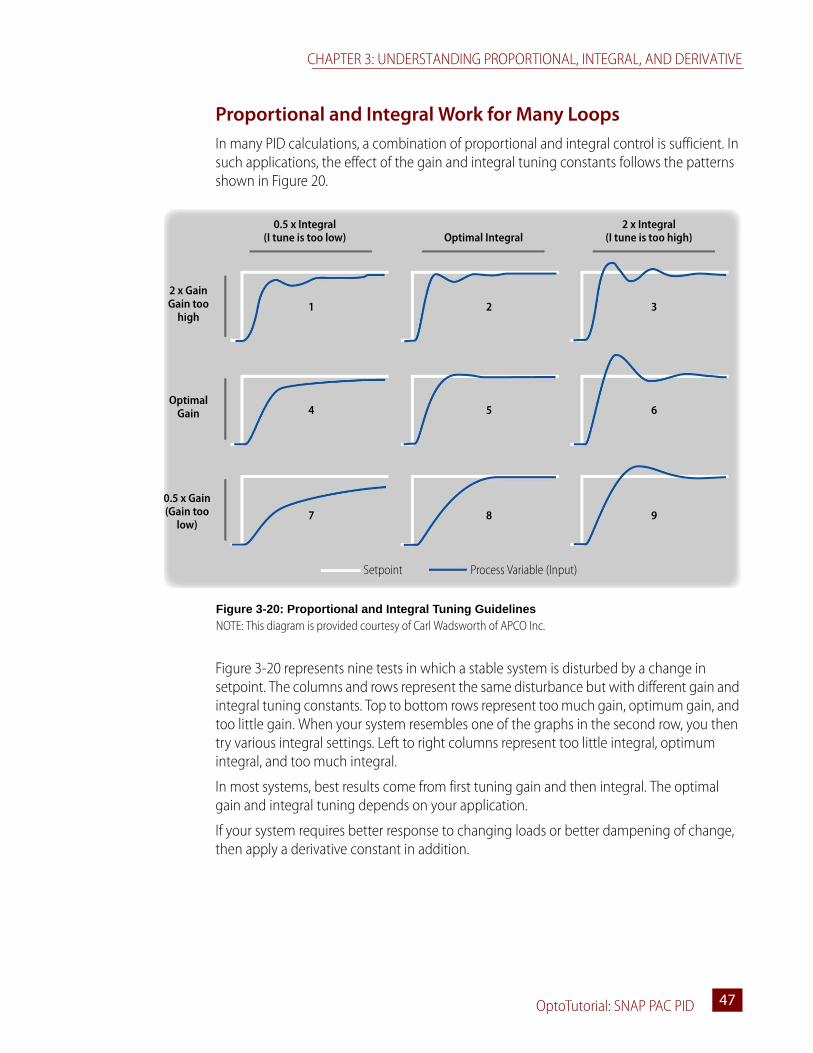
Proportional and Integral Work for Many LoopsIn many PID calculations, a combination of proportional and integral control is sufficient. In such applications, the effect of the gain and integral tuning constants follows the patterns shown in Figure 20.
Figure 3-20 represents nine tests in which a stable system is disturbed by a change in setpoint. The columns and rows represent the same disturbance but with different gain and integral tuning constants. Top to bottom rows represent too much gain, optimum gain, and too little gain. When your system resembles one of the graphs in the second row, you then try various integral settings. Left to right columns represent too little integral, optimum integral, and too much integral.
In most systems, best results come from first tuning gain and then integral. The optimal gain and integral tuning depends on your application.
If your system requires better response to changing loads or better dampening of change, then apply a derivative constant in addition.
Figure 3-20: Proportional and Integral Tuning Guidelines
NOTE: This diagram is provided courtesy of Carl Wadsworth of APCO Inc.
2 x Integral(I tune is too high)Optimal Integral
0.5 x Integral(I tune is too low)
2 x Gain Gain too
high
Optimal Gain
0.5 x Gain (Gain too
low)
Setpoint Process Variable (Input)
1 2 3
4
7
5
8
6
9

CONCEPTS
OptoTutorial: SNAP PAC PID48
Understanding DerivativeA derivative term is based on the rate of change in the process variable. The measurement of derivative produces a term that increases or decreases the controller output based on the speed at which the process variable is approaching or moving away from setpoint.
Mathematically, the derivative is a line that is tangential to the graph of the process variable at a point in time. By analyzing the slope of the line, which way it points and how steep it is, the derivative term adjusts the controller output.
Like integral, a true mathematical derivative may require more processing power than the PID calculation needs, so the measurement is simplified, and tuning parameters help correct for the estimate (as well as adjust the algorithm to the unique needs of a real system).
Figure 3-21: Influence of the Derivative on Controller Output
Mathematical Derivative
Derivative becomes more influential to the controller output.
Derivative contribution will try to reduce any over-correction.
Derivative contribution becomes less influential.
Process Variable
Setpoint

CHAPTER 3: UNDERSTANDING PROPORTIONAL, INTEGRAL, AND DERIVATIVE
OptoTutorial: SNAP PAC PID 4949
In the ISA, Parallel and Interacting algorithms, the final D term is based on the slope multiplied by a ratio of the D tuning parameter to the scan interval.
Figure 3-22: Derivative Measurement in ISA, Parallel, and Interact-ing Algorithms
Derivative Measurement in ISA, Parallel, and Interacting Algorithms
Scan interval
Process Variable
Setpoint
Derivative measurement calculates the slope of a line between the current and previous process variables.
Previous process variable Current process
variable
The D constant will either increase or decrease the influence of the slope, depending on 1) whether Tune D is greater or less than the system interval, and 2) whether the scan interval is greater than 1.
Slope of line

CONCEPTS
OptoTutorial: SNAP PAC PID50
In the Velocity algorithms, the final D term is based on the difference between the current slope and the previous slope multiplied by a ratio of the D tuning parameter to the scan interval. This is similar to the other algorithms, but the last two slopes are considered in the calculation of the D term.
Considerations for Choosing Derivative Tuning ParametersWhen tuning the D constant, these considerations apply:
• Many loops work adequately without a D term. Use a D term to reduce overshooting of the setpoint or in applications that have a long system dead time.
• When choosing a D tuning value, be aware of your scan interval. The D term may differ in magnitude depending on whether your D tuning constant is smaller or larger than your scan interval.
Figure 3-23: Derivative Measurement in Velocity Algorithms
Derivative Measurement in Velocity Algorithms
Process Variable
PV_2
The D constant will either increase or decrease the influence of the slope, depending on 1) whether Tune D is greater or less than the system interval, and 2) whether the scan interval is greater than 1.
PV_1
Current Process Variable (PV)
The Velocity algorithms calculate the difference between the last two slopes.
Previous slope
Current slope
Scan Interval
Current slope minus previous slope
Difference between slopes

CHAPTER 3: UNDERSTANDING PROPORTIONAL, INTEGRAL, AND DERIVATIVE
OptoTutorial: SNAP PAC PID 5151
• Try D tune values close to your scan interval, and observe the effects of higher and lower values.
Activity 2: Tune a PIDThere is no absolute way to tune a PID loop, as systems vary. In many applications, safety has to be considered first and precautions made to prevent a process from becoming unstable or equipment from being damaged. Each system will have its own safety requirements, which you must determine. In addition, PID loops from different manufacturers will behave differently.
All specific tuning parameters cited in this lesson apply to the Learning Center’s PID simulator, which is safe when used properly.
Preparation: Configure PID LoopIn Activity 1, you configured the minimum features needed to monitor the system dead time. Then you modified the scan rate so that it was one-third the system dead time.
In this activity, you will tune the PID loop on the SNAP PAC Learning Center. Before proceeding, make sure your configuration settings are set as described below.1. In Configure mode, open the PID loop configuration.
a. In the Strategy Tree, right-click the PID Control_Tank_Temperature.b. Select Modify.
2. Provide PID configuration.a. Enter the following information:
Input: I/O Point – TemperatureInput low range: 0Input high range: 100Setpoint: Host – 0 (Initial value)Output: I/O Point Output lower clamp: 0Output upper clamp: 100Algorithm: ISAAlthough you can use any of the algorithms, a non-Velocity algorithm is chosen for this activity to demonstrate steady-state error. Unlike the ISA, Parallel and Interacting algorithms, the Velocity algorithms require an initial integral constant (in addition to gain), which may prevent the steady-state error that this activity intends to demonstrate.Mode: ManualScan Rate: 0.4

ACTIVITY 2: TUNE A PID
OptoTutorial: SNAP PAC PID52
Gain: –5A final gain constant will be determined by tuning, but before you can tune your PID, your gain constant must be either a positive or negative according to the type of system you have. PAC Control’s PID algorithms calculate error by subtracting setpoint from the input (PV – Input), therefore producing a negative error when heat needs to be applied. To convert the error to the appropriate output, gain must be a negative value.
3. Download and run your strategy.
Determine Ambient Temperature and SetpointYou will tune the gain by observing the response to a setpoint increase of 5° F above ambient temperature. Before doing this, you need to determine the ambient temperature and arrange your graph so that you can easily see the effect of the setpoint change on the input. 1. In Debug mode, double-click the PID icon on the Strategy Tree.
The View PID Loop dialog box appears with the setpoint, process variable (input), and controller output plotted in real time. (As your loop should be in manual mode, disregard the setpoint and output values at this time.)
2. In the Output field, type 0 and click Apply.3. Wait for your temperature value to stabilize.
Tune I: 0Tune D: 0
b. Click OK to close the Edit PID Loop dialog box.

CHAPTER 3: UNDERSTANDING PROPORTIONAL, INTEGRAL, AND DERIVATIVE
OptoTutorial: SNAP PAC PID 5353
The following steps are based on an ambient temperature of 75° F degrees. Hopefully, your ambient temperature isn’t too far from this.
4. Change your setpoint.
5. Adjust the span of the input axis to 10 percent.
a. In the Setpoint field, type a value that is 5° F warmer than ambient temperature. For example, if your ambient temperature is 75, type 80.
b. Click Apply.
a. Click Input Axis.b. Choose View 10% Span.
ACTIVITY 2: TUNE A PID
OptoTutorial: SNAP PAC PID54
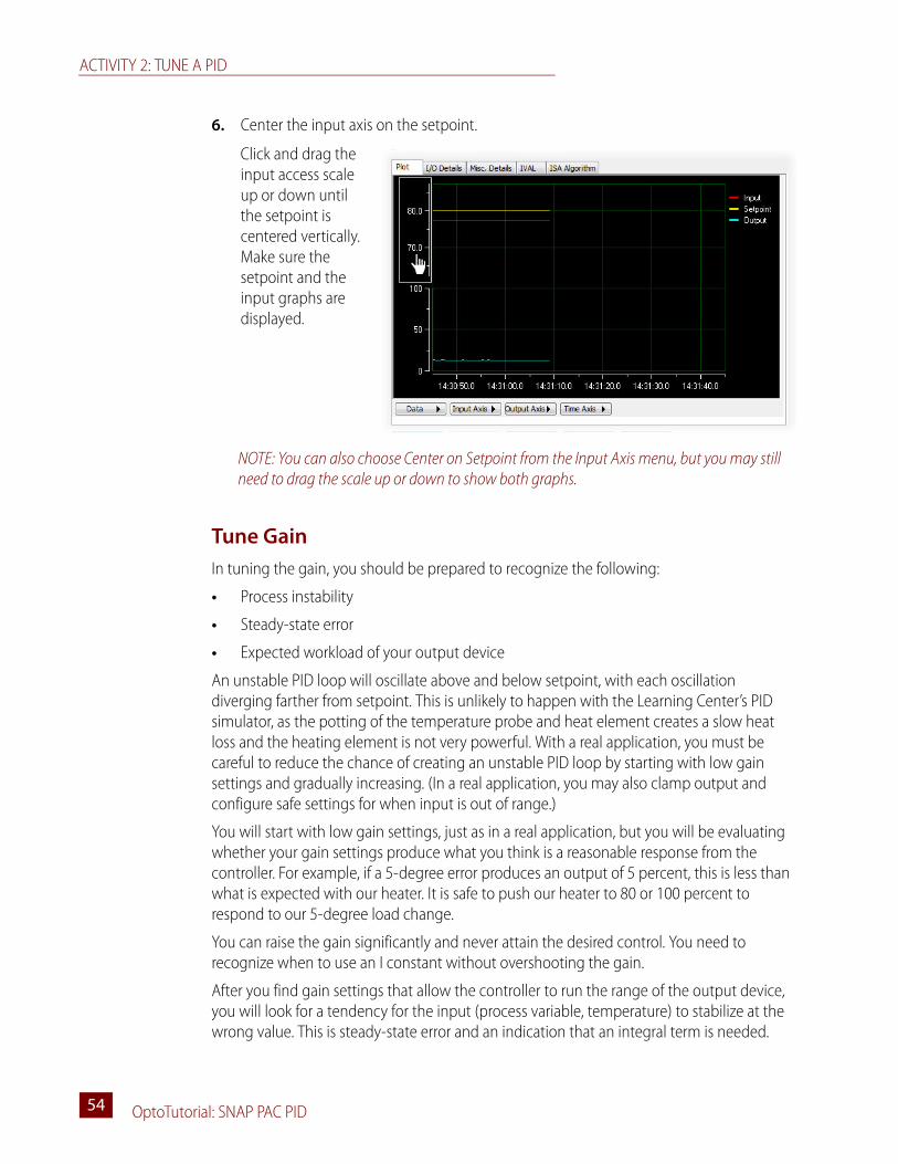
6. Center the input axis on the setpoint.
NOTE: You can also choose Center on Setpoint from the Input Axis menu, but you may still need to drag the scale up or down to show both graphs.
Tune GainIn tuning the gain, you should be prepared to recognize the following:
• Process instability
• Steady-state error
• Expected workload of your output device
An unstable PID loop will oscillate above and below setpoint, with each oscillation diverging farther from setpoint. This is unlikely to happen with the Learning Center’s PID simulator, as the potting of the temperature probe and heat element creates a slow heat loss and the heating element is not very powerful. With a real application, you must be careful to reduce the chance of creating an unstable PID loop by starting with low gain settings and gradually increasing. (In a real application, you may also clamp output and configure safe settings for when input is out of range.)
You will start with low gain settings, just as in a real application, but you will be evaluating whether your gain settings produce what you think is a reasonable response from the controller. For example, if a 5-degree error produces an output of 5 percent, this is less than what is expected with our heater. It is safe to push our heater to 80 or 100 percent to respond to our 5-degree load change.
You can raise the gain significantly and never attain the desired control. You need to recognize when to use an I constant without overshooting the gain.
After you find gain settings that allow the controller to run the range of the output device, you will look for a tendency for the input (process variable, temperature) to stabilize at the wrong value. This is steady-state error and an indication that an integral term is needed.
Click and drag the input access scale up or down until the setpoint is centered vertically. Make sure the setpoint and the input graphs are displayed.

CHAPTER 3: UNDERSTANDING PROPORTIONAL, INTEGRAL, AND DERIVATIVE
OptoTutorial: SNAP PAC PID 5555
1. In the Mode field, select Auto and click Apply.
Observe the response of the controller. Typically, you’ll notice that the controller output drops before this setpoint is reached, and therefore a gain of –5 is too low.
2. Try various increases in gain.a. Type –10 in the Gain field.b. Click Apply.
Observe the input and the output levels. Output is still low—approximately 40 percent.
c. Type -30 in the Gain field.d. Click Apply.
The white arrows (added to the screen capture) show the effect of a gain of –5: an error of 4 produces an output that is 20 percent of what the heater is capable of. Your result may be different, but clearly the output is not sufficient, as the temperature is too low.
ACTIVITY 2: TUNE A PID
OptoTutorial: SNAP PAC PID56
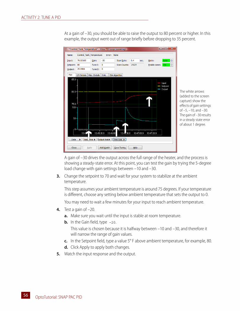
At a gain of –30, you should be able to raise the output to 80 percent or higher. In this example, the output went out of range briefly before dropping to 35 percent.
A gain of –30 drives the output across the full range of the heater, and the process is showing a steady-state error. At this point, you can test the gain by trying the 5-degree load change with gain settings between –10 and –30.
3. Change the setpoint to 70 and wait for your system to stabilize at the ambient temperature.
This step assumes your ambient temperature is around 75 degrees. If your temperature is different, choose any setting below ambient temperature that sets the output to 0.
You may need to wait a few minutes for your input to reach ambient temperature.
4. Test a gain of –20. a. Make sure you wait until the input is stable at room temperature.b. In the Gain field, type –20.
This value is chosen because it is halfway between –10 and –30, and therefore it will narrow the range of gain values.
c. In the Setpoint field, type a value 5° F above ambient temperature, for example, 80.d. Click Apply to apply both changes.
5. Watch the input response and the output.
The white arrows (added to the screen capture) show the effects of gain settings of –5, –10, and –30. The gain of –30 results in a steady state error of about 1 degree.

CHAPTER 3: UNDERSTANDING PROPORTIONAL, INTEGRAL, AND DERIVATIVE
OptoTutorial: SNAP PAC PID 5757
Wait for the input to stabilize.
In the example shown here, the gain of –20 resulted in an initial controller output of about 80 percent, which quickly diminished. If you compare this graph to the graph in Step 2 (on page 55), you’ll see that gains of –20 and –30 have a similar result: both drive the input to within 2° F of setpoint. Since a gain of –30 is not more effective than a gain of –20, it’s reasonable to suspect that we have reached the useful limit of gain. (NOTE: Because of differences in your environment and equipment, you may achieve this point with a different gain setting.)
Measure the Steady State Error1. Click Data and choose Cursor to display the cursor.2. Right-click the data cursor displayed in the PID plot and choose Style > Delta Y.3. Drag measurement bars to setpoint and to input.
a. Click and drag the upper red cursor to the setpoint graph.

ACTIVITY 2: TUNE A PID
OptoTutorial: SNAP PAC PID58
b. Click and drag the lower red cursor to the input graph.
In this example, the steady state error is about 1.5° F below setpoint, and a gain of -20 yields an output around 80 percent of the range of the output device. At this point it is reasonable to deploy an integral term to correct for the steady-state error.
Apply an Integral Tuning Constant to Correct Steady-State ErrorIn the ISA algorithm, the gain will multiply the integral (and derivative) terms.

CHAPTER 3: UNDERSTANDING PROPORTIONAL, INTEGRAL, AND DERIVATIVE
OptoTutorial: SNAP PAC PID 5959
In the Integral field, type 0.1 and click Apply.
In this example, an integral constant of 0.1 corrected the offset and continued to maintain the input close to setpoint with gradual changes in the output:
If your results are different, try higher or lower integral values, for example, 0.05 or 0.2. Also be aware that reducing the offset within a degree is acceptable, especially if your ambient temperature is fluctuating. You do not need to get perfect results, as the final tuning involves testing the tuning parameters against load changes.
Two of three objectives are being met with these tuning parameters:
• The setpoint is being maintained.
NOTE: In this activity, all screens showing a PID loop’s response to setpoint changes represent actual tests. This test was done when the ambient temperature dropped to 73° F, and so a setpoint of 78 was used.
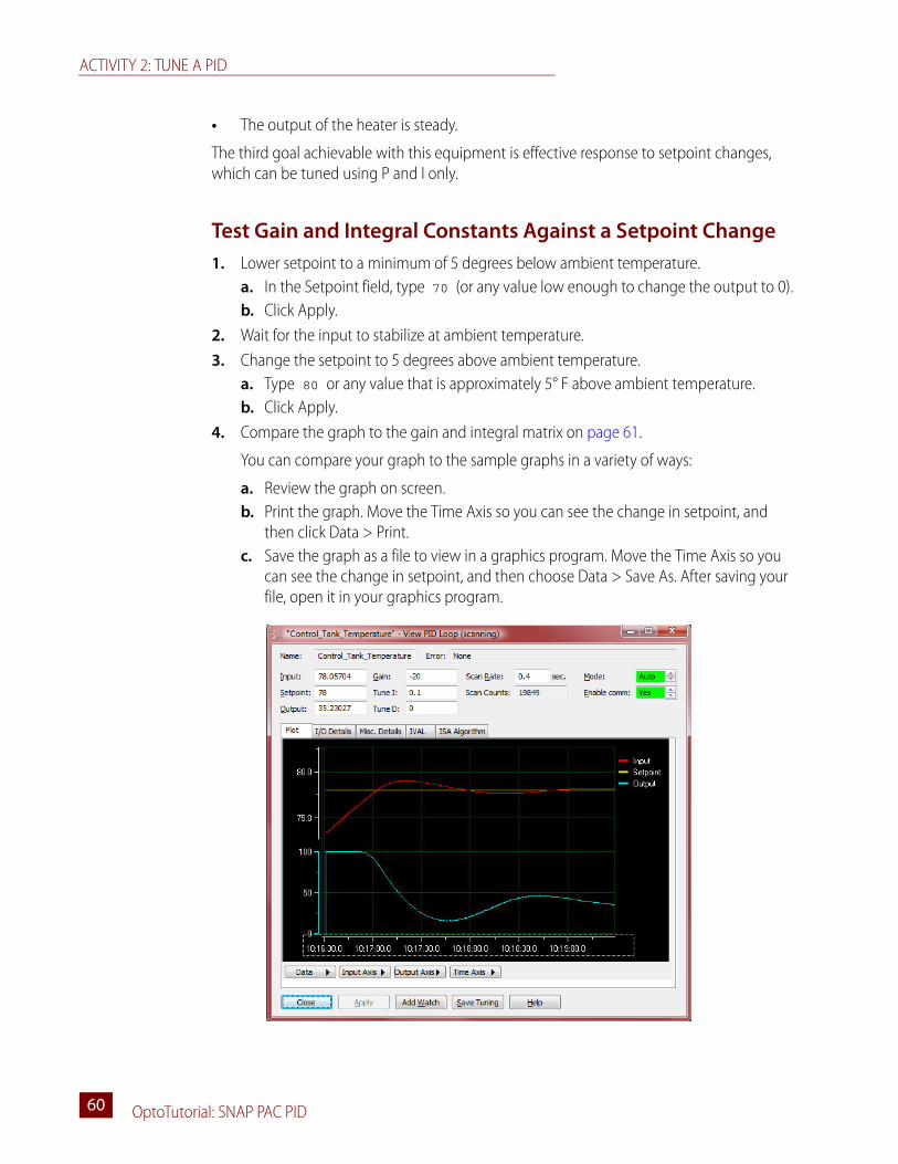
ACTIVITY 2: TUNE A PID
OptoTutorial: SNAP PAC PID60
• The output of the heater is steady.
The third goal achievable with this equipment is effective response to setpoint changes, which can be tuned using P and I only.
Test Gain and Integral Constants Against a Setpoint Change1. Lower setpoint to a minimum of 5 degrees below ambient temperature.
a. In the Setpoint field, type 70 (or any value low enough to change the output to 0).b. Click Apply.
2. Wait for the input to stabilize at ambient temperature.3. Change the setpoint to 5 degrees above ambient temperature.
a. Type 80 or any value that is approximately 5° F above ambient temperature.b. Click Apply.
4. Compare the graph to the gain and integral matrix on page 61.
You can compare your graph to the sample graphs in a variety of ways:
a. Review the graph on screen. b. Print the graph. Move the Time Axis so you can see the change in setpoint, and
then click Data > Print.c. Save the graph as a file to view in a graphics program. Move the Time Axis so you
can see the change in setpoint, and then choose Data > Save As. After saving your file, open it in your graphics program.
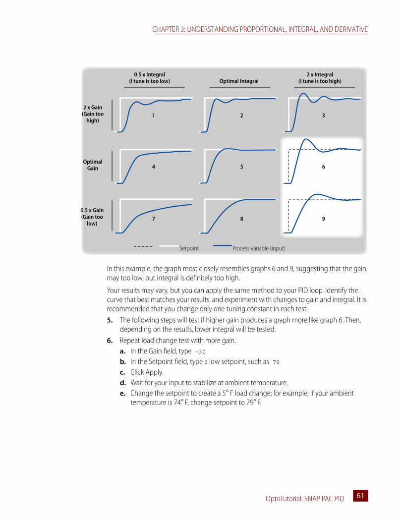
CHAPTER 3: UNDERSTANDING PROPORTIONAL, INTEGRAL, AND DERIVATIVE
OptoTutorial: SNAP PAC PID 6161
In this example, the graph most closely resembles graphs 6 and 9, suggesting that the gain may too low, but integral is definitely too high.
Your results may vary, but you can apply the same method to your PID loop. Identify the curve that best matches your results, and experiment with changes to gain and integral. It is recommended that you change only one tuning constant in each test.5. The following steps will test if higher gain produces a graph more like graph 6. Then,
depending on the results, lower integral will be tested. 6. Repeat load change test with more gain.
a. In the Gain field, type –30b. In the Setpoint field, type a low setpoint, such as 70c. Click Apply.d. Wait for your input to stabilize at ambient temperature.e. Change the setpoint to create a 5° F load change; for example, if your ambient
temperature is 74° F, change setpoint to 79° F.
2 x Integral(I tune is too high)Optimal Integral
0.5 x Integral(I tune is too low)
2 x Gain (Gain too
high)
Optimal Gain
0.5 x Gain (Gain too
low)
Setpoint Process Variable (Input)
1 2 3
4
7
5
8
6
9
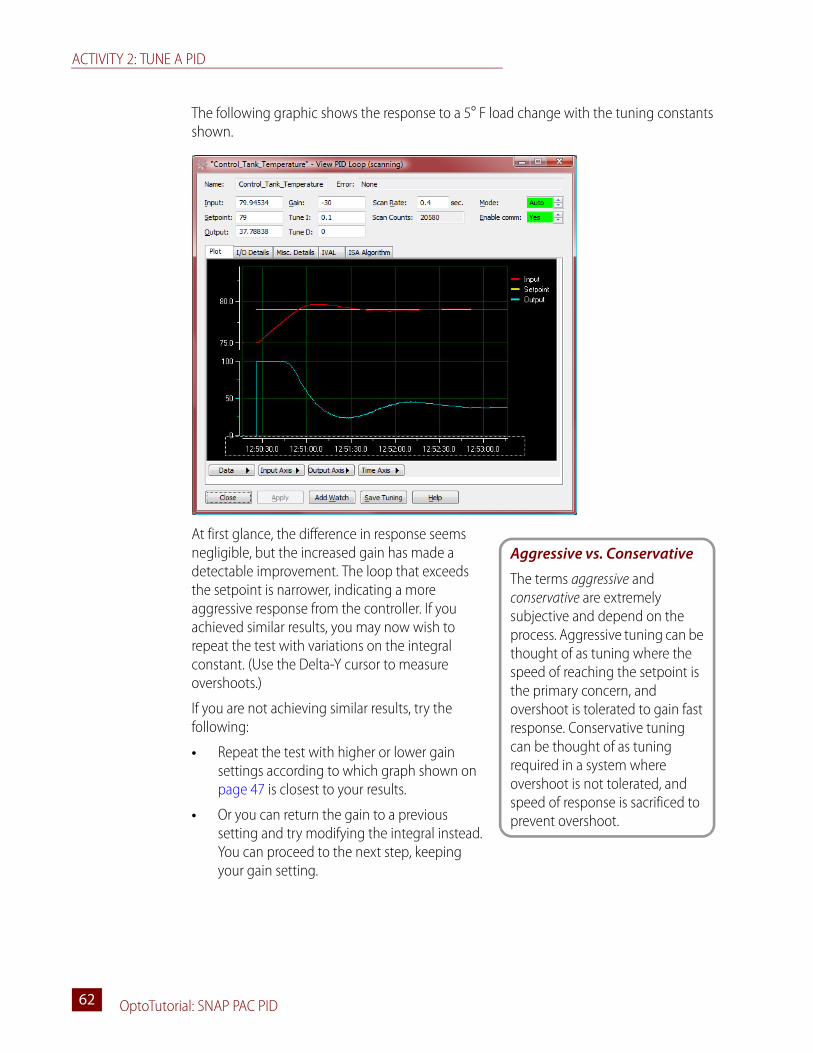
ACTIVITY 2: TUNE A PID
OptoTutorial: SNAP PAC PID62
The following graphic shows the response to a 5° F load change with the tuning constants shown.
At first glance, the difference in response seems negligible, but the increased gain has made a detectable improvement. The loop that exceeds the setpoint is narrower, indicating a more aggressive response from the controller. If you achieved similar results, you may now wish to repeat the test with variations on the integral constant. (Use the Delta-Y cursor to measure overshoots.)
If you are not achieving similar results, try the following:
• Repeat the test with higher or lower gain settings according to which graph shown on page 47 is closest to your results.
• Or you can return the gain to a previous setting and try modifying the integral instead. You can proceed to the next step, keeping your gain setting.
Aggressive vs. Conservative
The terms aggressive and conservative are extremely subjective and depend on the process. Aggressive tuning can be thought of as tuning where the speed of reaching the setpoint is the primary concern, and overshoot is tolerated to gain fast response. Conservative tuning can be thought of as tuning required in a system where overshoot is not tolerated, and speed of response is sacrificed to prevent overshoot.
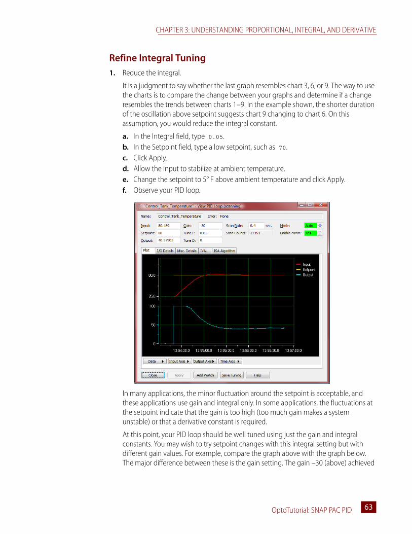
CHAPTER 3: UNDERSTANDING PROPORTIONAL, INTEGRAL, AND DERIVATIVE
OptoTutorial: SNAP PAC PID 6363
Refine Integral Tuning1. Reduce the integral.
It is a judgment to say whether the last graph resembles chart 3, 6, or 9. The way to use the charts is to compare the change between your graphs and determine if a change resembles the trends between charts 1–9. In the example shown, the shorter duration of the oscillation above setpoint suggests chart 9 changing to chart 6. On this assumption, you would reduce the integral constant.
a. In the Integral field, type 0.05.b. In the Setpoint field, type a low setpoint, such as 70.c. Click Apply.d. Allow the input to stabilize at ambient temperature.e. Change the setpoint to 5° F above ambient temperature and click Apply.f. Observe your PID loop.
In many applications, the minor fluctuation around the setpoint is acceptable, and these applications use gain and integral only. In some applications, the fluctuations at the setpoint indicate that the gain is too high (too much gain makes a system unstable) or that a derivative constant is required.
At this point, your PID loop should be well tuned using just the gain and integral constants. You may wish to try setpoint changes with this integral setting but with different gain values. For example, compare the graph above with the graph below. The major difference between these is the gain setting. The gain –30 (above) achieved

ACTIVITY 2: TUNE A PID
OptoTutorial: SNAP PAC PID64
a better response to the load change. A gain setting of –20 resulted in a slower response.
2. Click Save Tuning to save your tuning parameters.
Tune DerivativeDerivative is not necessary for this loop, and it is likely that you will not improve the loop’s performance with a D tuning constant. But to examine the effect of derivative constants, do the following:
1. Make sure your PID setpoint is at 5° F above ambient temperature.
(It should be from previous steps.)
2. Set the view the Input Axis to 1 percent of span.
This will allow you to see minor changes affected by the derivative term.
3. Use the Delta-Y Cursor to measure error.4. Apply D tuning constant.
a. In the Tune D field, type 0.1 and click Apply. b. Observe the graph for a minute.
5. Try various settings from 0.1 to 10.
For the purpose of examining the derivative term, you may wish to return your Gain and Integral tuning constants to previous, less-effective settings and then compare

CHAPTER 3: UNDERSTANDING PROPORTIONAL, INTEGRAL, AND DERIVATIVE
OptoTutorial: SNAP PAC PID 6565
these with variations of derivative. For example, a derivative of 10 makes a noticeable difference in keeping the input near the setpoint.
Follow-upThis tutorial has provided a basic introduction to the concepts behind PID control and some hands-on practice using PAC Control’s PID features. With the basic skills taught in this tutorial, you should be able to explore many other features on your own. Here are a few areas you may wish to start with:
• Repeat the tuning process with each of the four PID algorithms. To select a different algorithm, return to Configure mode.
• Try Min. Change and Max. Change settings to simulate output devices that need their operation restricted.
• Experiment with Feed Forward constants.
Many PID systems are effectively controlled with Gain and Integral constants only and no Derivative constant. In this example, the Gain and Integral settings are maintaining the temperature at 0.07 from setpoint. To demonstrate the effect of the derivative constant, the resolution of the Input axis was increased to show a 1 percent span. At this resolution, the plot reveals changes of 0.01 degrees F.
The left side of the plot shows the effect of Gain at -30, Integral at 0.1, and no Derivative constant. The arrow shows when a Derivative constant of 10 was applied. The right side of the plot shows how the Derivative constant is keeping the input closer to setpoint. However, the biggest difference is the spikes in the output. Factors to consider are whether it’s more important to have precise adherence to setpoint or to have steady output. Spikes in the output can cause mechanical stress on your process or accelerate device failure times.

ACTIVITY 2: TUNE A PID
OptoTutorial: SNAP PAC PID66
• View the real-time calculations during Debug mode.
• Simulate the effect of cascading loops, where one loop controls the setpoint of another. You can configure the setpoint to the Learning Center’s potentiometer to simulate a frequently changing setpoint.

SNAP PAC Learning Center User’s Guide 6767
Appendix A
Reference
Configuring a PID LoopA PID loop is configured in PAC Control’s Configure mode.
• Name: Type a unique, descriptive name for the PID.
• Description: A description of the PID is optional.

CONFIGURING A PID LOOP
Optotutorial: SNAP PAC PID68
• Input: The process variable being monitored by the PID loop. Input options are I/O Point, Host, or PID Output.
– Choose I/O Point if this PID will get its process variable from an I/O point, and then choose an I/O point from the drop-down list of configured points (or type a point name to configure a new point on the same I/O unit).
– Choose Host if this PID will get its process variable from PAC Control, for example, from a PID or I/O point on another I/O unit, or from a process variable that must be manipulated before use in the PID loop. Type an initial value for the Input.
– Choose PID if this PID is getting its process variable from the output of another PID on this brain (used in cascading control loops). Choose a PID from the drop-down list of configured PID loops on this brain.
• Square Root: If you chose I/O Point or PID for step C, you can check this box if you wish the error to be calculated based on the square root of the process variable. (This is applicable to flow control systems where volumetric flow is proportional to the square root of a signal from a flow transducer.)
• Low Range and High Range: Set the valid range of the process variable by typing a number for the low range and the high range. This range tells the PID what is valid input and is also used to create a Span term that aligns the input and output scales; therefore this range affects the tuning of the PID loop. (Options for responding to out-of-range input are described under Output options for when input is out of range.)
• Setpoint: Choose the source for the setpoint: I/O point, Host, or PID Output.
– Choose I/O Point if you wish to control the setpoint using a device such as a potentiometer, and then choose an I/O point from the drop-down list of configured points (or type a point name to configure a new point).
– Choose Host if you wish to control setpoint using PAC Control or PAC Display™, for example, from a PID or I/O point on another I/O unit, or from a process variable that must be manipulated before use in the PID loop. Type an initial value for the Input.
– Choose PID Output if this PID is part of a cascading control system in which another PID loop on the brain will control the setpoint of this PID Loop.
• Output: Choose the destination for the controller output: I/O Point or Host.
– Choose I/O Point to use an output point to correct the process variable (input), and then choose an I/O point from the drop-down list of configured points (or type a point name to configure a new point).
– Choose Host to use the output for controlling the setpoint or input to another PID.
The output can be preset or changed at any time through PAC Control by first switching to Manual mode. For example, if you have determined that the output should start at 40 percent whenever the system is activated, switch to Manual mode and then set the PID output to this value. Then switch back to Auto mode.
• Lower Clamp and Upper Clamp: Set the valid range of the output by typing a number for the Lower and Upper Clamp. This range tells the PID what is valid output
APPENDIX A: REFERENCE
Optotutorial: SNAP PAC PID 6969
and is also used to create a Span term that aligns the input and output scales; therefore this range affects the tuning of the PID loop.
Setting clamps is particularly important if the device controlled by the output signal has “dead areas” at either end. For example, say the output is scaled 0-10. It is connected to a valve that begins to open at 1.25 and is “effectively” fully open at 5.75 (even though it may only be 70 percent open). Set Lower Clamp to 1.2 (valve closed) and Upper Clamp to 5.75 (valve effectively fully open). This prevents reset windup, potentially resulting in dramatically improved control when the output value has reached either limit and has to suddenly reverse direction.
The upper and lower clamp settings prevent the output from exceeding a desirable range. Minimally, these should correspond to the range of an output point (for example, the heater is scaled to 0 to 100 percent and so the lower and upper clamps are 0 and 100).
These settings can also be used to ensure that the output device doesn’t shut off (for example, keeping a heater or circulation pump running regardless of the PID output) or that the output never reaches a destructively high setting (for example, keeping a burner or motor below maximum).
• Minimum Change and Maximum Change: (Optional) The minimum and maximum change allow you to do two things:
– Minimum Change allows you to prevent an output device from turning on until there is a minimum desirable workload. For example, you may not want the heater to turn on to correct a 1 degree error, only to quickly turn off again. A value of 0 disables Minimum change.
– Maximum Change allows you to prevent undesirable effects from too drastic a change in output. For example, you could use this to moderate the increase in a pump’s output to prevent pipe breakage. A value of 0 disables Maximum Change.
The Minimum Change and Maximum Change are for each scan period, and therefore these settings may be a factor in choosing your scan rate.
• Output options for when input is out of range: In the event that the input variable goes out of range, you can instruct the PID to 1) freeze output at the current value, 2) switch to Manual mode and stay there until PAC Control logic or an operator intervenes, 3) set output at a desired minimum or maximum, or both 2 and 3 (set the output and go to Manual mode).
– For 1, leave these options unchecked.
– For 2 only, check Switch to manual mode when input goes out of range.
– For 3 only, check Force output when input is out of range and type output values for when the input is below or above the range. (NOTE: This action is independent of 2, meaning the output can be forced and the PID can be switched to Manual mode; however, when the PID is being operated in Manual mode, this feature is not active.)
– For 2 and 3, check both options and type out-of-range values.

CONFIGURING A PID LOOP
Optotutorial: SNAP PAC PID70
• Algorithm: Select a PID algorithm: Velocity B, Velocity C, ISA, Parallel, Interacting.
• Mode: Auto activates the PID. Manual is for debugging and requires you to control the PID output.
• Scan Rate (Scan Interval): The scan interval is the first and one of the most important parameters to set. This setting specifies how often (in seconds) the PID loop will scan the input and calculate an output. The minimum value is 0.001 (1 ms). Factors to consider are 1) system dead time and 2) tasks on the brain competing for processing power. Special equipment limitations may require a long scan interval, but generally, scan interval should be shorter than one-third the duration of the system dead time.
• Gain: Gain enables the controller to implement a proportional response to the error. The Proportional Gain (P) acts directly on the change in error since the last output calculation. Type a positive or negative number for gain. Heating systems require a negative number and cooling systems a positive number. Gain is usually refined during the tuning process. Higher gain results in increased output change. Too much gain results in output oscillation. Too little gain results in slow performance.
Depending on the algorithm, gain may also be used as a multiplier on the integral term, the derivative term, or both.
• Integral: Integral corrects steady-state error common with proportional control. A positive integral value is required. Integral that is too low results in undershooting the setpoint. Integral that is too high results in overshoot, oscillation, or both.
By multiplying the integral by the scan time, the PID loop will provide the same integral action even if the scan interval is changed. For example, if the integral part of the PID loop moves the output 1 percent every second on a scan interval of 1 second, then if the scan interval is changed to 0.1 second, it will still result in a change of output of 1 percent every second, but it will be implemented as 0.1 percent every 0.1 second.
• Derivative: The derivative contributes an appropriate value to the output that is consistent with where the input will be at the next scan if it continues at its current rate of change.
Derivative is used in feed forward applications and in systems where the loop dead time is long. Most applications that do not have long dead times and long time constants are not significantly helped by derivative, and it can be counterproductive. Most PID loops in industry are run as PI loops.
To disable derivative, set its tuning constant to zero.
• Feed Forward Initial and Feed Forward Gain are constants that are multiplied and added to the controller output.
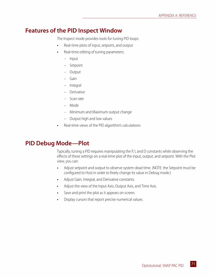
APPENDIX A: REFERENCE
Optotutorial: SNAP PAC PID 7171
Features of the PID Inspect WindowThe Inspect mode provides tools for tuning PID loops:
• Real-time plots of input, setpoint, and output
• Real-time editing of tuning parameters:
– Input
– Setpoint
– Output
– Gain
– Integral
– Derivative
– Scan rate
– Mode
– Minimum and Maximum output change
– Output high and low values
• Real-time views of the PID algorithm’s calculations
PID Debug Mode—PlotTypically, tuning a PID requires manipulating the P, I, and D constants while observing the effects of these settings on a real-time plot of the input, output, and setpoint. With the Plot view, you can:
• Adjust setpoint and output to observe system dead time. (NOTE: the Setpoint must be configured to Host in order to freely change its value in Debug mode.)
• Adjust Gain, Integral, and Derivative constants.
• Adjust the view of the Input Axis, Output Axis, and Time Axis.
• Save and print the plot as it appears on screen.
• Display cursors that report precise numerical values.

PID DEBUG MODE—PLOT
Optotutorial: SNAP PAC PID72
Features of the Plot
Setpoint and Input plot. Adjust resolution using Input Axis menu below the plot. Click and drag to move the focus.
Output plot. Adjust resolution using the Output Axis menu below the plot. Click and drag to move the focus.
Time axis. Adjust resolution using the Time Axis menu below the plot. Click and drag left or right to move the focus.
Input, Setpoint, and Output. These fields can be edited when set to Host. Output can also be edited when Mode is set to Manual.
PID tuningMode option for activating (Auto) and deactivating (Manual) the PID.
Option for enabling or disabling communication between the I/O unit and the
control engine. This feature also reflects whether the strategy is running.
Any changes to settings must be applied to take effect.
Save tuning to update the PID configuration with the current settings.
Add Watch allows you to select the following PID values for inclusion in a Watch Window: input, setpoint, output, gain, integral constant, derivative constant, system interval and mode.

APPENDIX A: REFERENCE
Optotutorial: SNAP PAC PID 7373
Moving a Plot’s Scale
Displaying CursorsChoose Cursor under the Data menu to display numeral data. Cursors allow you to drag vertical or horizontal lines to identify Input, Setpoint, Output, or Time values. Once displayed you can drag the red line to the desired place on the plot.
You can click and drag the Input, Output, and Time axes. White arrows show the direction to drag the scale and are not part of the plot.
The X-Y Cursor displays the time and value of the selected Y axis (for example, Input). Change the selected Y axis to Setpoint, Output, or Input by right-clicking the cursor and choosing Channel from the pop-up menu.

PID DEBUG MODE—PLOT
Optotutorial: SNAP PAC PID74
Changing the Cursor SettingsYou can right-click the cursor information box to change the cursor.
Using Delta-X and Delta-Y CursorsThe Delta X cursor displays the difference in time between two vertical red lines. Each red line can be dragged to a different position, as shown by the arrows (which are not part of the plot).
Selecting the data represented in the cursor
Selecting the cursor function

APPENDIX A: REFERENCE
Optotutorial: SNAP PAC PID 7575
Resetting TrackingWhen you manipulate the time axis of the cursors, the plot remains as a fixed point. To restore the view of the current values, choose Reset Scale Tracking under the Time Axis menu.
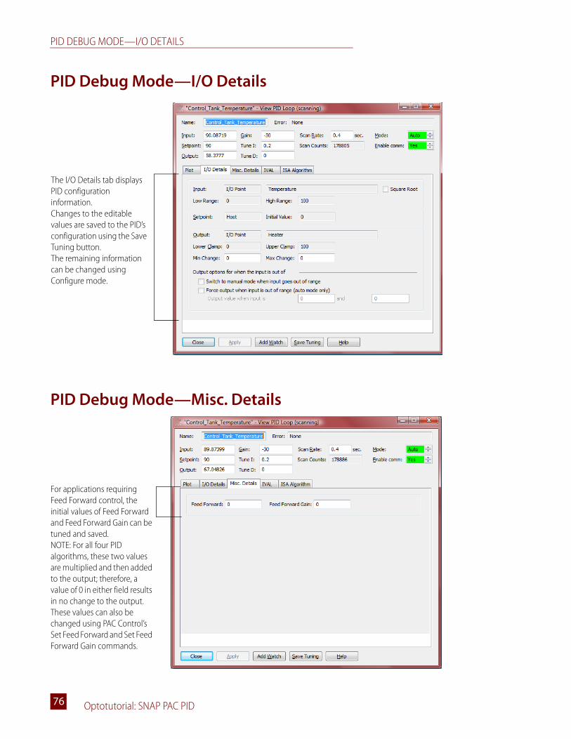
PID DEBUG MODE—I/O DETAILS
Optotutorial: SNAP PAC PID76
PID Debug Mode—I/O Details
PID Debug Mode—Misc. Details
The I/O Details tab displays PID configuration information.Changes to the editable values are saved to the PID’s configuration using the Save Tuning button.The remaining information can be changed using Configure mode.
For applications requiring Feed Forward control, the initial values of Feed Forward and Feed Forward Gain can be tuned and saved. NOTE: For all four PID algorithms, these two values are multiplied and then added to the output; therefore, a value of 0 in either field results in no change to the output.These values can also be changed using PAC Control’s Set Feed Forward and Set Feed Forward Gain commands.
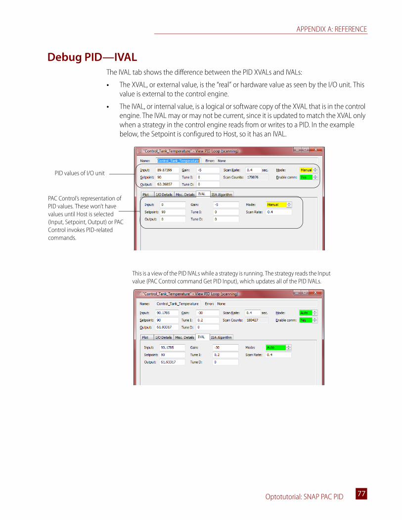
APPENDIX A: REFERENCE
Optotutorial: SNAP PAC PID 7777
Debug PID—IVALThe IVAL tab shows the difference between the PID XVALs and IVALs:
• The XVAL, or external value, is the “real” or hardware value as seen by the I/O unit. This value is external to the control engine.
• The IVAL, or internal value, is a logical or software copy of the XVAL that is in the control engine. The IVAL may or may not be current, since it is updated to match the XVAL only when a strategy in the control engine reads from or writes to a PID. In the example below, the Setpoint is configured to Host, so it has an IVAL.
PID values of I/O unit
PAC Control’s representation of PID values. These won’t have values until Host is selected (Input, Setpoint, Output) or PAC Control invokes PID-related commands.
This is a view of the PID IVALs while a strategy is running. The strategy reads the Input value (PAC Control command Get PID Input), which updates all of the PID IVALs.
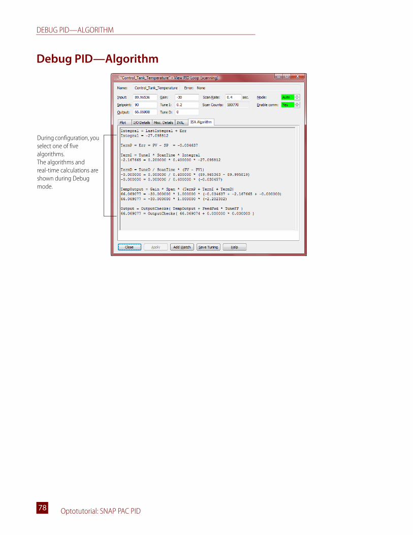
DEBUG PID—ALGORITHM
Optotutorial: SNAP PAC PID78
Debug PID—Algorithm
During configuration, you select one of five algorithms.The algorithms and real-time calculations are shown during Debug mode.
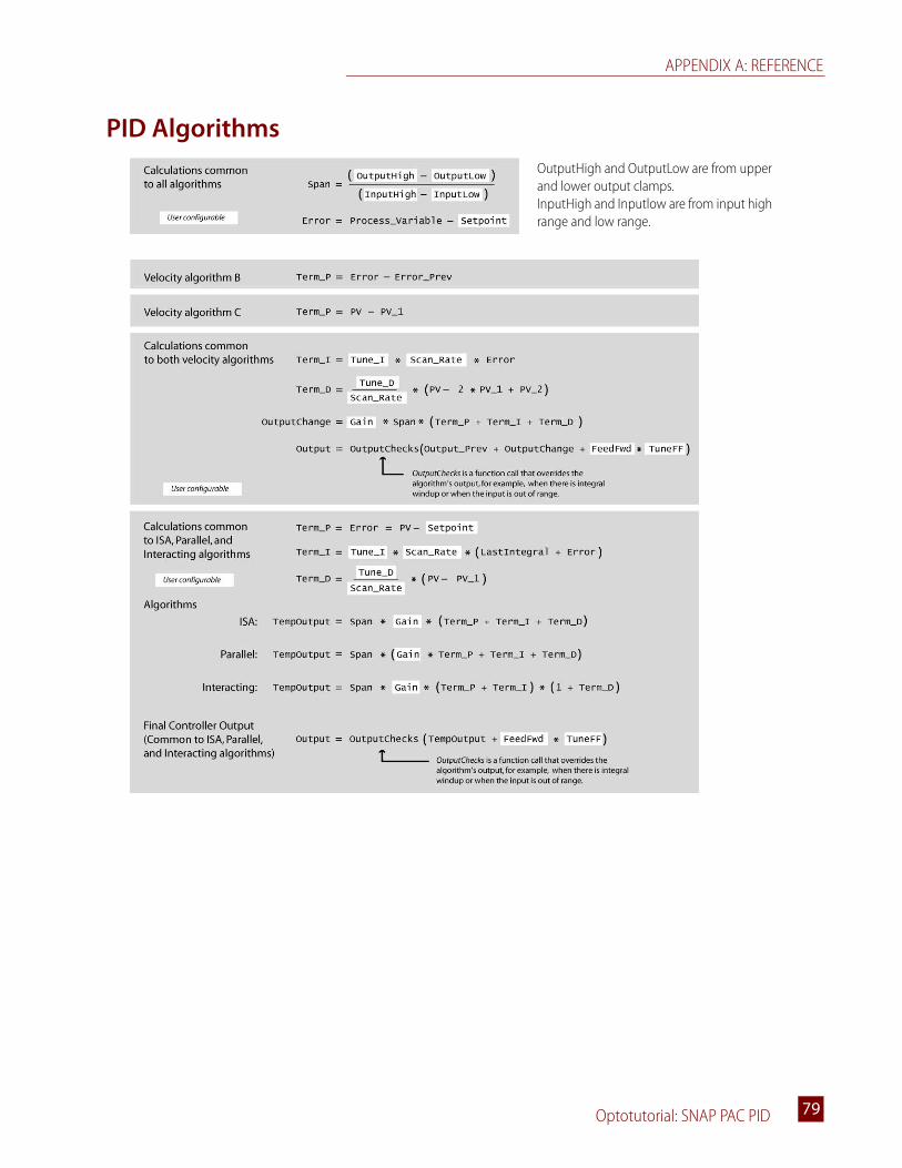
APPENDIX A: REFERENCE
Optotutorial: SNAP PAC PID 7979
PID AlgorithmsOutputHigh and OutputLow are from upper and lower output clamps.InputHigh and Inputlow are from input high range and low range.

DEFINING A NEW CONTROL ENGINE
Optotutorial: SNAP PAC PID80
Defining a New Control EngineThis tutorial assumes that you have completed the SNAP PAC Learning Center lessons and therefore have created a control engine. A control engine resides on the PC workstation and is a reference for PAC Control to communicate with the PAC R1 brain. If you are working on a different computer, you will need to define a new control engine. 1. In the strategy tree, right-click Control Engines and click Add.2. In the Configure Control Engines dialog box, click Add.3. In the Select Control Engine dialog box, click Add to open the Control Engine
Configuration dialog box.
4. In the Control Engine Name field, type any name, for example SNAP PAC R 5. Type the IP address of your SNAP PAC, for example 10.0.4.106. Click OK.
You can now associate your Control Engine.