Topic #8

16.30/31 Feedback Control Systems

State-Space Systems

• System Zeros

• Transfer Function Matrices for MIMO systems

� �

� �

Fall 2010 16.30/31 8–1

Zeros in State Space Models

• Roots of transfer function numerator called the system zeros.

• Need to develop a similar way of defining/computing them using a state space model.

• Zero: generalized frequency s0 for which the system can have a non-zero input u(t) = u0e

s0t, but exactly zero output y(t) ≡ 0 ∀t

• Note that there is a specific initial condition associated with this response x0, so the state response is of the form x(t) = x0e

s0t

u(t) = u0es0t x(t) = x0e

s0t y(t) ≡ 0⇒ ⇒

• Given x = Ax + Bu, substitute the above to get:

x0s0es0t = Ax0e

s0t + Bu0es0t

� s0I − A −B

� x0 = 0 ⇒ u0

• Also have that y = Cx + Du = 0 which gives:

Cx0es0t + Du0e

s0t = 0 � C D

� x0 = 0 → u0

• So we must find the s0 that solves: � � � � s0I − A −B x0 = 0

C D u0

• Is a generalized eigenvalue problem that can be solved in MATLAB using eig.m or tzero.m 1

1MATLAB is a trademark of the Mathworks Inc.

October 17, 2010

� �

� � � �

� �

Fall 2010 16.30/31 8–2

• There is a zero at the frequency s0 if there exists a non-trivial solution of � �

s0I − A −B det = 0

C D

• Compare with equation on page 6–??

x0 • Key Point: Zeros have both direction u0

and frequency s0

• Just as we would associate a direction (eigenvector) with each pole (frequency λi)

s+2 • Example: G(s) = s2+7s+12

−7 −12 1 � � A = B = C = 1 2 D = 0

1 0 0

⎡ ⎤ � � s0 + 7 12 −1det

s0I − A −B = det ⎣ −1 s0 0 ⎦

C D 1 2 0

= (s0 + 7)(0) + 1(2) + 1(s0) = s0 + 2 = 0

so there is clearly a zero at s0 = −2, as we expected. For the directions, solve: ⎡ ⎤ ⎡ ⎤ ⎡ ⎤⎡ ⎤

s0 + 7 12 −1 x01 5 12 −1 x01 ⎣ −1 s0 0 ⎦ ⎣ x02 ⎦ = ⎣ −1 −2 0 ⎦⎣ x02 ⎦ = 0? 1 2 0 u0 1 2 0 u0 s0=−2

gives x01 = −2x02 and u0 = 2x02 so that with x02 = 1

x0= −2

and u = 2e−2t

1

October 17, 2010

Fall 2010 16.30/31 8–3

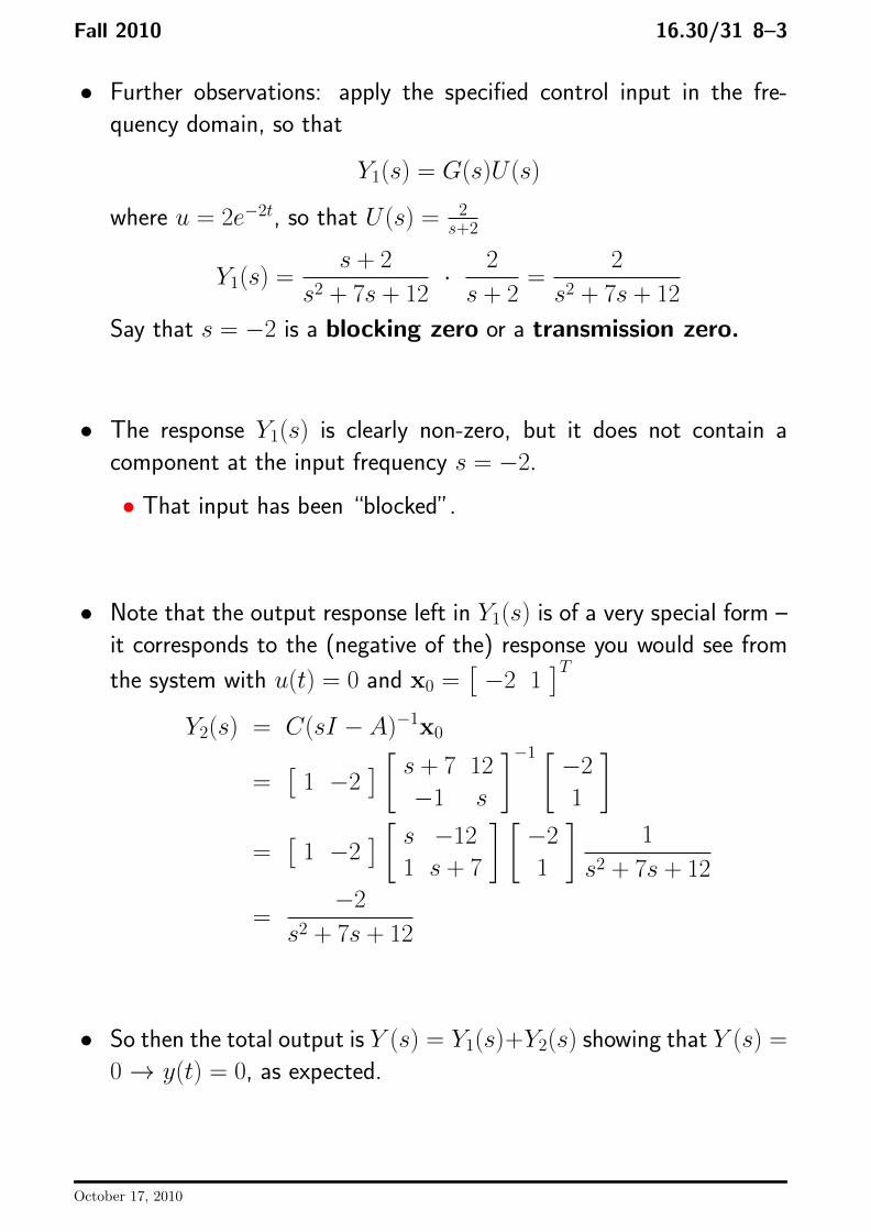
• Further observations: apply the specified control input in the fre­quency domain, so that

Y1(s) = G(s)U(s)

where u = 2e−2t, so that U(s) = 2 s+2

s + 2 2 2 Y1(s) = =

s2 + 7s + 12 · s + 2 s2 + 7s + 12

Say that s = −2 is a blocking zero or a transmission zero.

• The response Y1(s) is clearly non-zero, but it does not contain a component at the input frequency s = −2.

• That input has been “blocked”.

• Note that the output response left in Y1(s) is of a very special form – it corresponds to the (negative of the) response you would see from � �T the system with u(t) = 0 and x0 = −2 1

Y2(s) = C(sI − A�)−1 x0 �−1 � � � � s + 7 12 −2 = 1 −2 −1 s 1 � � � � � � s −12 −2 1 = 1 −2

1 s + 7 1 s2 + 7s + 12 −2

= s2 + 7s + 12

• So then the total output is Y (s) = Y1(s)+Y2(s) showing that Y (s) = 0 y(t) = 0, as expected. →

October 17, 2010

� �

Fall 2010 16.30/31 8–4

Simpler Test

• Simpler test using transfer function matrix:

• If z is a zero with (right) direction [ζT , uT ]T , then � � � � zI − A − B ζ

= 0 C D u

• If z not an eigenvalue of A, then ζ = (zI − A)−1Bu, which gives

C(zI − A)−1B + D u = G(z)u = 0

• Which implies that G(s) loses rank at s = z

• If G(s) is square, can find the zero frequencies by solving:

det G(s) = 0

• If any of the resulting roots are also eigenvalues of A, need to re-check the generalized eigenvalue matrix condition.

• Need to be very careful when we find MIMO zeros that have the same frequency as the poles of the system, because it is not obvious that a pole/zero cancelation will occur (for MIMO systems).

• The zeros have a directionality associated with them, and that must “agree” as well, or else you do not get cancelation

• More on this topic later when we talk about controllability and observability

October 17, 2010

Fall 2010 16.30/31 8–5

Transfer Function Matrix

• Note that the transfer function matrix (TFM) notion is a MIMO generalization of the SISO transfer function

It is a matrix of transfer functions • ⎤⎡

G(s) =⎣g11(s) g1m(s)· · ·

. . . ⎦

gp1(s) gpm(s)· · ·

• gij(s) relates input of actuator j to output of sensor i.

• It is relatively easy to go from a state-space model to a TFM, but not obvious how to go back the other way.

• Simplest approach is to develop a state space model for each element of gij(s) in the form Aij, Bij, Cij, Dij, and then assemble (if TFM is p × m)

⎤⎡⎤⎡ A11 B11

A=

⎢⎢⎢⎢⎢⎢⎢⎣

. . .A1m

A21...

⎥⎥⎥⎥⎥⎥⎥⎦

B =

⎢⎢⎢⎢⎢⎢⎢⎣B21

⎥⎥⎥⎥⎥⎥⎥⎦

. . .

.

B1m

.. Apm Bpm⎤⎡ ⎢⎢⎢⎣

C11 C1m· · · C21

. . . C2m ⎥⎥⎥⎦

C= D = [Dij]... Cp1 · · · Cpm

October 17, 2010

���������

���������

Fall 2010 16.30/31 8–6

• One issue is how many poles are needed - this realization might be inefficient (larger than necessary).

• Related to McMillan degree, which for a proper system is the degree of the characteristic polynomial obtained as the least com­mon denominator of all minors of G(s). 2

• Subtle point: consider a m × m matrix A, then the standard minors formed by deleting 1 row and column and taking the de­terminant of the resulting matrix are called the m − 1th order minors of A.

• To consider all minors of A, must consider all possible orders, i.e. by selecting j ≤ m subsets of the rows and columns and taking the resulting determinant.

• Given an n × m matrix A with entries aij, a minor of A is the determinant of a smaller matrix formed from its entries by selecting only some of the rows and columns.

• Let K = { k1 k2 . . . kp } and L = { l1 l2 . . . lp } be subsets of {1, 2, . . . , n} and {1, 2, . . . ,m}, respectively.

• Indices are chosen so k1 < k2 · · · < kp and l1 < l2 · · · < lp.

• pth order minor defined by K and L is the determinant 3

[A]K,L =

ak1l1 ak1l2 . . . ak1lp

ak2l1 ak2l2 . . . ak2lp ... . . .

akpl1 akpl2 . . . akplp

• If p = m = n then the minor is simply the determinant of the matrix.

• In a nutshell what this means is that a 2 × 2 matrix has 4 order-1 minors and 1 order-2 minor to consider.

2Lowest order polynomial that can be divided cleanly by all denominators of the minors of G(s).

3See here for details

October 17, 2010

Fall 2010 16.30/31 8–7

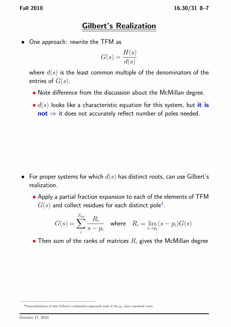
Gilbert’s Realization

• One approach: rewrite the TFM as

H(s)G(s) =

d(s)

where d(s) is the least common multiple of the denominators of the entries of G(s).

• Note difference from the discussion about the McMillan degree.

• d(s) looks like a characteristic equation for this system, but it is not it does not accurately reflect number of poles needed. ⇒

• For proper systems for which d(s) has distinct roots, can use Gilbert’s realization.

• Apply a partial fraction expansion to each of the elements of TFM G(s) and collect residues for each distinct pole4 .

Nm� RiG(s) = where Ri = lim (s − pi)G(s)

is − pi s→pi

• Then sum of the ranks of matrices Ri gives the McMillan degree

4Generalizations of this Gilbert’s realization approach exist if the gij have repeated roots.

October 17, 2010

� �

Fall 2010 16.30/31 8–8

• Can develop a state space realization by analyzing each element of the partial fraction expansion

• Set Ri = CiBi, and find appropriate Bi and Ci

• Form Ai by placing the poles on the diagonal as many times as needed (determined by rank of Ri)

• Form state space model: ⎡ ⎤ ⎡ ⎤ A1 B1

.x = ⎣ . . . ⎦ x + ⎣ .. ⎦ u ANm BNm

y = C1 CNm x· · ·

October 17, 2010

� �

�

� � � � �

Fall 2010 16.30/31 8–9

Zero Example 1 ⎤⎡

• TFM G(s) =

⎢⎢⎢⎢⎣

1 1s + 2 s + 2

1 s − 2 s − 2 (s + 1)(s + 2)

⎥⎥⎥⎥⎦

• To compute the McMillan degree for this system, form all minors (4 order-1 and 1 order-2):

1 1 1 s − 2 2 − 7s s + 2

,s + 2

,s − 2

, (s + 1)(s + 2)

, (s − 2)(s + 1)(s + 2)2

• To find LCD (least common multiple of denominators), pull out small­est polynomial that leaves all terms with no denominator:

1 (s − 2)(s + 1)(s + 2)2

{(s − 2)(s + 1)(s + 2), (s − 2)(s + 1)(s + 2),

(s + 1)(s + 22), (s − 2)2(s + 2), 2 − 7s

• So we expect a fourth order system with poles at s = 2, s = −2 (two), and s = −1

• Compare with the Gilbert realization, find d(s): ⎤⎡ (s + 1)(s − 2) (s + 1)(s − 2)

1 G(s) =

(s + 1)(s + 2)(s − 2) ⎢⎣

⎥⎦2( + 1)( + 2) ( 2)−s s s �

1 0 0 1 0 0 1 1 1 = + +

s + 1 0 −3 s − 2 1 0 (s + 2) 0 4

• Note that the rank of the last 2×2 matrix is 2

• So the system order is 4 - we need to have two poles s = −2.

October 17, 2010

� �

� � � �

Fall 2010 16.30/31 8–10

So the system model for the example is • � � 0 A1 = [−1] B1 = 0 −3 C1 =

1 −2 0 1 1

A2 = B2 = C2 = I2 0 0 4−2 � � � � 0

A3 = [2] B3 = 1 0 C3 = 1

Note, realization model on 8–5 would be 5th order, not 4th. •

Code: MIMO Models

1 %2 % basic MIMO TFM to SS3 %4 G=tf({1 1;1 [1 −2]},{[1 2] [1 2];[1 −2] [1 3 2]});5

6 % find residue matrices of the 3 poles7 R1=tf([1 1],1)*G;R1=minreal(R1);R1=evalfr(R1,−1)8 R2=tf([1 2],1)*G;R2=minreal(R2);R2=evalfr(R2,−2)9 R3=tf([1 −2],1)*G;R3=minreal(R3);R3=evalfr(R3,2)

10

11 % form SS model for 3 poles using the residue matrices 12 A1=[−1];B1=R1(2,:);C1=[0 1]'; 13 A2=[−2 0;0 −2];B2=R2;C2=eye(2); 14 A3=[2];B3=R3(2,:);C3=[0 1]'; 15

16 % combine submodels 17 A=zeros(4);A(1:1,1:1)=A1;A(2:3,2:3)=A2;A(4,4)=A3; 18 B=[B1;B2;B3]; 19 C=[C1 C2 C3]; 20

21 syms s 22 Gn=simple(C*inv(s*eye(4)−A)*B); 23

24 % alternative is to make a SS model of each g {ij}25 A11=−2;B11=1;C11=1; 26 A12=−2;B12=1;C12=1; 27 A21=2;B21=1;C21=1; 28 A22=[−3 −2;1 0];B22=[2 0]';C22=[0.5 −1]; 29

30 % and then combine 31 AA=zeros(5);AA(1,1)=A11;AA(2,2)=A12;AA(3,3)=A21;AA(4:5,4:5)=A22; 32 BB=[B11 B11*0;B12*0 B12;B21 B21*0;B22*0 B22]; 33 CC=[C11 C12 zeros(1,3);zeros(1,2) C21 C22]; 34 GGn=simple(CC*inv(s*eye(5)−AA)*BB); 35

36 Gn,GGn

October 17, 2010

� �

� � � �

Fall 2010 16.30/31 8–11

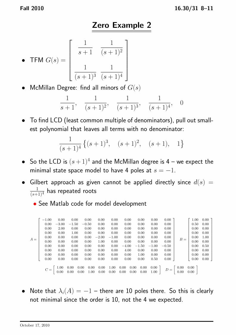
Zero Example 2 ⎤⎡

• TFM G(s) =

⎢⎢⎢⎢⎣

1 1s + 1 (s + 1)2

1 1(s + 1)3 (s + 1)4

⎥⎥⎥⎥⎦

• McMillan Degree: find all minors of G(s)

1 1 1 1 , , , , 0

s + 1 (s + 1)2 (s + 1)3 (s + 1)4

• To find LCD (least common multiple of denominators), pull out small­est polynomial that leaves all terms with no denominator:

1(s + 1)3 , (s + 1)2 , (s + 1), 1

(s + 1)4

• So the LCD is (s +1)4 and the McMillan degree is 4 – we expect the minimal state space model to have 4 poles at s = −1.

• Gilbert approach as given cannot be applied directly since d(s) = 1

(s+1)4 has repeated roots

• See Matlab code for model development

⎤⎡⎤⎡ −1.00 0.00 0.00 0.00 0.00 0.00 0.00 0.00 0.00 0.00 0.00

1.00 0.00

A =

⎢⎢⎢⎢⎢⎢⎢⎢⎢⎢⎢⎢⎢⎢⎣

⎥⎥⎥⎥⎥⎥⎥⎥⎥⎥⎥⎥⎥⎥⎦

B =

⎢⎢⎢⎢⎢⎢⎢⎢⎢⎢⎢⎢⎢⎢⎣

⎥⎥⎥⎥⎥⎥⎥⎥⎥⎥⎥⎥⎥⎥⎦

−3.00 −1.50 −0.50 0.00 0.00 0.00 0.00 0.00 0.00 2.00 0.00 0.00

0.50 0.00 0.00 0.00 0.00 0.00 0.00 1.00 0.00 0.00 0.00 0.50 0.00 0.00 0.00 0.00

0.00 0.00 0.00 0.00 0.00 0.00 0.00 0.00 0.00 1.00 0.00 0.00 0.00 0.00 0.00 0.00 0.00 0.00 0.00 0.00 0.00 −2.00 −1.00 0.00 0.00 0.00 0.00

1.00 0.000.00 0.00 0.00 0.00 0.00 0.00 0.00 0.00 0.00 0.00 0.00 0.00 0.00 0.00 −4.00 −1.50 −1.00 −0.50

4.00 0.00 0.00 0.000.00 0.00 0.00 0.00 0.00 0.00 0.00 0.00 0.00 0.00 0.00 0.00 0.00 1.00 0.00 0.00 0.00 0.00 0.00 0.00 0.00 0.00 0.00 0.00 0.50 0.00 0.00 0.00

1.00 0.00 0.00 0.00 0.00 1.00 0.00 0.00 0.00 0.00 0.00 0.00 C = D =

0.00 0.00 0.00 1.00 0.00 0.00 0.00 0.00 0.00 1.00 0.00 0.00

• Note that λi(A) = −1 – there are 10 poles there. So this is clearly not minimal since the order is 10, not the 4 we expected.

October 17, 2010

Fall 2010 16.30/31 8–12

Matlab command minreal can be used to convert to a minimal• realization. � � � � −0.40 −0.16 −1.00 0.01 0.23 −0.02

A = 0.32 0.50

−1.49 −1.06

−0.06 −1.17

1.07 −0.39 B = −0.97

−0.05 0.36

−0.31 −0.07 0.16 0.02 −0.94 0.01 −0.75

� � � �

C = 0.18

−1.11 −1.01 −0.29

0.35 0.43

−0.63 −0.28

D = 0.00 0.00

0.00 0.00

• New model has 6 states removed - so the minimal degree is 4 as expected.

Code: Zeros (zero example1.m)

1 G1=ss(tf({1 1;1 1},{[1 1] conv([1 1],[1 1]);conv([1 1],conv([1 1],[1 1])) ...2 conv([1 1],conv([1 1],conv([1 1],[1 1])))})); %3 [a,b,c,d]=ssdata(G1);4 latex(a,'%.2f','nomath') %5 latex(b,'%.2f','nomath') %6 latex(c,'%.2f','nomath') %7 latex(d,'%.2f','nomath') %8 G2=minreal(G1);[a2,b2,c2,d2]=ssdata(G2);9 latex(a2,'%.2f','nomath') %

10 latex(b2,'%.2f','nomath') %11 latex(c2,'%.2f','nomath') %12 latex(d2,'%.2f','nomath') %

October 17, 2010

� �

� �

� � � �

� � � �

Fall 2010 16.30/31 8–13

Zero Example 3 ⎤⎡

• TFM G(s) =

⎢⎢⎢⎢⎣

2s + 3 3s + 5s2 + 3s + 2 s2 + 3s + 2

−10

(s + 1)

⎥⎥⎥⎥⎦

• McMillan Degree: find all minors of G(s)

2s + 3 ,

3s + 5 ,

−1 ,

−(3s + 5) s2 + 3s + 2 s2 + 3s + 2 (s + 1) (s + 1)(s2 + 3s + 2)

• To find LCD, pull out smallest polynomial that leaves all terms with no denominator:

1 (2s + 3)(s + 1), (3s + 5)(s + 1), −(s 2 + 3s + 2), −(3s + 5)

(s2 + 3s + 2)(s + 1)

• So the LCD is (s2 + 3s + 2)(s + 1) = (s + 1)2(s + 2)

• The McMillan degree is 3 – we expect the minimal state space model to have 3 poles.

• For Gilbert approach, we rewrite

2s + 3 3s + 5

G(s) = −(s + 2) 0

(s + 1)(s + 2) =

R1

s + 1 +

R2

s + 2

where 2s+3 3s+5 1 2

R1 = lim (s + 1)G(s) = lim s+2 s+2 =−1 0 −1

1 1

0s→−1 s→−1

2s+3 3s+5s+1 s+1R2 = lim (s + 2)G(s) = lim s+2 =

s→−2 s→−2 −s+1 0 0 0

which also indicates that we will have a third order system with 2 poles at s = −1 and 1 at s = −2.

October 17, 2010

� �

� �

Fall 2010 16.30/31 8–14

For the state space model, note that • � �� � 1 2 1 0

R1 = = C1B1 −1 0 0 1

1 � � R2 = 1 1 = C2B20

giving ⎡ ⎤ ⎡ ⎤ −1 0 0 1 0

0 ⎦ B = ⎣ 0 1 ⎦A = ⎣ 0 −1 0 0 −2 1 1

1 2 1 C = −1 0 0

• From Matlab you get: ⎡ ⎤ ⎡ ⎤ −1.00 0.00 0.00 0.56 1.12

A = ⎣ 0.00 −2.00 0.00 ⎦ B = ⎣ 0.35 0.35 ⎦

0.00 0.00 −1.00 0.50 0.00 � � � � 1.79 2.83 0.00 0.00 0.00

C = D = 0.00 0.00 −2.00 0.00 0.00

Code: Zeros (zero example2.m)

1 G1=ss(tf({[2 3] [3 5];−1 0},{[1 3 2] [1 3 2];[1 1] 1})); % 2 G1=canon(G1,'modal') 3 [a,b,c,d]=ssdata(G1); 4 latex(a,'%.2f','nomath') % 5 latex(b,'%.2f','nomath') % 6 latex(c,'%.2f','nomath') % 7 latex(d,'%.2f','nomath') %

October 17, 2010

� �

Fall 2010 16.30/31 8–15

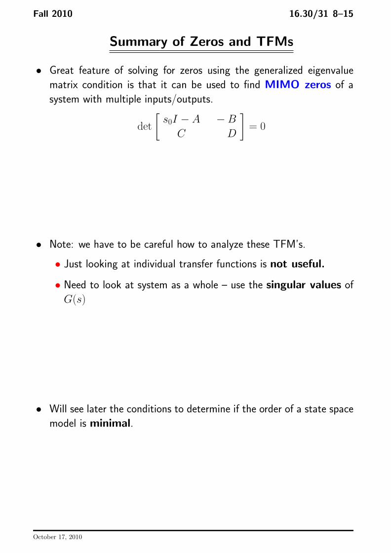
Summary of Zeros and TFMs

• Great feature of solving for zeros using the generalized eigenvalue matrix condition is that it can be used to find MIMO zeros of a system with multiple inputs/outputs.

s0I − A − B det = 0

C D

• Note: we have to be careful how to analyze these TFM’s.

• Just looking at individual transfer functions is not useful.

• Need to look at system as a whole – use the singular values of G(s)

• Will see later the conditions to determine if the order of a state space model is minimal.

October 17, 2010

MIT OpenCourseWarehttp://ocw.mit.edu

16.30 / 16.31 Feedback Control Systems Fall 2010

For information about citing these materials or our Terms of Use, visit: http://ocw.mit.edu/terms.