16 Spreadsheet Applications - MG Codemaroulis.mgcode.gr/wp-content/uploads/2013/05/fpeo16.pdf ·...

523

16 Spreadsheet Applications

16.1 IntroductIon

General purpose spreadsheet software can be used effectively for engineering calculations. For example, Microsoft Excel with Visual Basic for Applications is an effective tool for process design. Spreadsheets offer sufficient process model “hospitality.” They are connected easily and online with charts and graphic objects, resulting in powerful and easy-to-use graphical interfaces. Excel also supports mathematical and statistical tools. For instance, Solver is an excellent tool for solving sets of equations and performing optimization. Databases are effectively and easily accessed. In addition, Visual Basic for Applications offers a powerful object-oriented programming language capable of constructing commercial graph-ics interfaces.

Our book Food Process Design (Maroulis and Saravacos, 2003) presents a sys-tematic approach to solve engineering problems in a spreadsheet environment. In particular, it shows integrated procedures for robust process design by analyzing the following topics:

• Modeling and spreadsheets• Analyzing the Solver• Sensitivity analysis using Excel tables• Controls and Dialog boxes to input data• Graphics to get results• Databases• Visual Basic as a programming language

In the present book, a more simplified concept is adopted. It is a step from classic hand calculations toward more sophisticated spreadsheet calculations.

The following topics are introduced and applied to problems similar to those of the previous chapters of this book.

• Name variables• Insert data• Insert equations using names• Use “Goal Seek” to solve an equation• Automate using Visual Basic• Assign a macro to a button• Use Excel tables• Use Excel charts• Use the scroll bars

83538_C016.indd 523 12/1/2010 1:05:03 AM

524 Food Process Engineering Operations

• Construct a simple database• Use Combo Boxes• Use matrix operations• Use Solver

16.2 Shell and tubeS heat exchanger

In this example, the following Excel operations are introduced:

• Name variables (Ctrl + Shift + F3)• Insert data• Insert equations using names

16.2.1 Problem Formulation

Calculate the appropriate shell and tube heat exchanger for a tomato paste heating process using the available heating steam.

The design specifications are

F = 1 kg/s Feed flow rate

T1 = 50°C Feed temperature

T2 = 100°C Target temperature

Ts = 120°C Steam temperature

The required data of the tomato paste and the heating steam are

ρ = 1130 kg/m3 Fluid density

λ = 0.55 W/(m K) Fluid thermal conductivity

η = 0.27 Pa s Fluid apparent viscosity

Cp = 3.50 kJ/(kg K) Specific heat

ΔHs = 2200 kJ/kg Latent heat of steam condensation

The following design variables are also assumed:

u = 1 m/s Fluid velocity in tubes

d = 0.01 m Tube diameter

dx = 5 mm Tube thickness

n = 4 Number of passes in tubes

16.2.2 Problem Solution

The thermal load is calculated by the equation

Q FC T Tp= −( )2 1

83538_C016.indd 524 12/1/2010 1:05:04 AM

Spreadsheet Applications 525

The required steam flow rate Q is calculated by the equation

Q F Hs s= ∆

The mean temperature difference ΔTm

∆T T T T T

T T T Tm

s s

s s

= − − −− −[ ]

( ) ( )ln ( ) / ( )

1 2

1 2

The total number of tubes N

u

F

N n d=

ρ π( )( )2 4

The surface heat transfer coefficient outside tubes ho

h

Nd

Fo

s

=

27501 3/

The Pr number

Pr

Cp=η

λ

The Re number

Re

d u= ρη

The Nu number

Nu

d

L=

1 861 3

./

RePrw

ηη

0.14

The surface heat transfer coefficient inside tubes hi

Nu

h di=λ

The overall heat transfer coefficient U

1 1 1U h hi o

= +

83538_C016.indd 525 12/1/2010 1:05:07 AM


AB

CD

EF

1Va

riab

leTe

xt N

ame

Exce

l Nam

eVa

lue

Uni

tsEq

uati

on2

Feed

flow

rate

FF

1kg

/s3

Feed

tem

pera

ture

T 1T

1.50

°C4

Targ

et te

mpe

ratu

reT 2

T2.

100

°C5

Stea

m te

mpe

ratu

reT s

Ts12

0°C

6Fl

uid

spec

ific

heat

Cp

Cp

3.50

kJ/k

gC7

Late

nt h

eat o

f ste

am c

onde

nsat

ion

ΔH

sdH

s22

00kJ

/kg

8Fl

uid

dens

ityρ

p_11

30K

g/m

3

9Fl

uid

ther

mal

con

duct

ivity

λk_

0.55

W/m

K10

Flui

d ap

pare

nt v

isco

sity

ηn_

0.27

Pa s

11Fl

uid

velo

city

in tu

bes

uu.

1.00

m/s

12Tu

be d

iam

eter

dd

0.01

m13

Tube

thic

knes

sδx

dx5

mm

14N

umbe

r of p

asse

s in

tube

sn

m4

—16

Ther

mal

load

QQ

175

kW:=

F*C

p*(T

2.−T

1.)

17St

eam

flow

rate

F sFs

0.08

kg/s

:=Q

/dH

s18

Mea

n te

mpe

ratu

re d

iffer

ence

ΔT

mdT

m40

°C:=

( (Ts

−T1.

)−(T

s−T

2.) )

/LN

( (Ts

−T1.

)/(T

s−T

2.) )

19To

tal n

umbe

r of t

ubes

NM

.45

—:=

F/p_

/(u.

/m)/

(3.1

4*dˆ

2/4)

20Su

rfac

e he

at tr

ansf

er c

oeffi

cien

t out

side

tube

sh o

ho4.

90kW

/m2 K

:=2.

75*(

M.*d

/Fs)

ˆ(1/

3)

21Pr

Num

ber

PrPr

1718

—:=

Cp*

n_/k

_*10

0022

Re N

umbe

rRe

Re42

—:=

u.*p

_*d/

n_23

Nu

Num

ber

Nu

Nu

9.28

—:=

1.86

*(Re

*Pr*

d/10

)ˆ(1

/3)*

1.2

24Su

rfac

e he

at tr

ansf

er c

oeffi

cien

t ins

ide

tube

sh i

hi0.

51kW

/m2 K

:=N

u*k_

/d/1

000

25O

vera

ll he

at tr

ansf

er c

oeffi

cien

tU

U0.

46kW

/m2 K

:=(1

/(1/

ho+1

/hi)

)27

Hea

t tra

nsfe

r are

aA

A9.

48m

2:=

Q/U

/dTm

28Sh

ell d

iam

eter

DD

.0.

20m

:=(d

+2*d

x/10

00)* (M

./0.3

19)ˆ

(1/2

.142

)29

Tube

leng

thL

L6.

70m

:=A

/M./3

.14/

d

FIg

ur

e 16

.1

83538_C016.indd 526 12/1/2010 1:05:07 AM


The total heat transfer area A

Q AU Tm= ∆

The shell diameter D

N

D

d=

0 3192 142

..

The tubes length L

A N dL= π

16.2.3 excel imPlementation

In an Excel spreadsheet and in the range A2:A29, type the names of the process variables incorporated in the previous solution as shown in Figure 16.1. The range A2:A14 is used for the data while the range A16:A29 for the results. In the next column and in the range B2:B29, type the symbols for these variables as used in the solution provided earlier.

In the range C2:C29, type the corresponding names in Excel. Use names simi-lar to their symbols in the text if possible. In the range E2:E29, type the corre-sponding units.

By selecting the range C2:D29 and by simultaneously pressing the buttons Ctrl + Shift + F3, the names in column C are assigned to the cells of column D (Figure 16.2).

Enter the data for the given variables in the range D2:D14. Enter the equations according to the previous solution procedure into the range D16:D29. These equa-tions are presented for information in the range F16:F29.

The problem has been solved. Any change of the data will change the result. The problem is solved with just 13 equations in the range D16:D29 by using 13 data in the range D2:D14. All other text in the spreadsheet is for information (Figure 16.1).

FIgure 16.2

83538_C016.indd 527 12/1/2010 1:05:08 AM


16.3 PSychrometrIc calculatIonS

In this example, the following simple Excel calculations are introduced:

• Use the Goal Seek function to solve an equation• Automate Using Simple Visual Basic• Assign a macro to a button


For an air/water mixture, when the following conditions are given:

P = 1 bar Pressure

T = 65°C Temperature

Y = 0.035 kg/kg db Total humidity (liquid + vapor)

Calculate the following properties:

Pd bar Dew pressure

Ps bar Vapor pressure at temperature T

Pw bar Vapor pressure at temperature Tw

Tb °C Boiling temperature

Td °C Dew temperature

Tw °C Wet bulb temperature

YL kg/kg db Humidity in liquid

YV kg/kg db Humidity in vapor

Ys kg/kg db Saturation humidity at temperature T

Yw kg/kg db Saturation humidity at temperature Tw

aw — Water activity

H kJ/kg db Enthalpy of humid air

CP kJ/kg K db Specific heat of humid air

ΔHS kJ/kg Latent heat of condensation of water vapor at temperature T

Suppose that the following data are valid:

m = 0.622 Air/water molecular weight ratio

CPA = 1.00 kJ/kg K Specific heat of air

CPV = 1.90 kJ/kg K Specific heat of water vapor

CPW = 4.20 kJ/kg K Specific heat of liquid water

ΔH0 = 2.50 MJ/kg Latent heat of water evaporation at 0°C

a1 = 1.19 × 101 Antoine equation constants for water

a2 = 3.99 × 103

a3 = 2.34 × 102

83538_C016.indd 528 12/1/2010 1:05:08 AM



A simple psychrometric model has been presented by Maroulis and Saravacos (2003) as follows:

PS = exp [a1 – a2/(a3 + T)] (E01)

YS = m PS/(P – PS) (E02)

YV = min (Y, YS) (E03)

YL = Y – YV (E04)

YV = mawPS/(P − awPS) (E05)

H = CPAT + YV (ΔH0 + CPV T) + YLCPLT (E06)

Tb = − a3 + a2/(a1 − ln P) (E07)

Td = a2/(a1 – ln[Y P/(m + Y)]) – a3 (E08)

Pd = exp[a1 – a2/(a3 + T)] (E09)

Pw = exp[a1 – a2/(a3 + Tw)] (E10)

Yw = mPw/(P – Pw) (E11)

CP = CPA + YV CPV (E12)

ΔHS = ΔH0 – (CPL – CPV)T (E13)

(YV – YW)/(T – TW) = – CP/ΔHS (E14)

Based on these equations, the following algorithm can be used:

(E01) → Ps

(E02) → Ys

(E03) → YV

(E04) → YL

(E05) → aw

(E06) → H

(E07) → Tb

(E08) → Td

(E09) → Pd

Tw Trial value ←(E10) → Pw

(E11) → Yw

(E12) → CP

(E13) → ΔHS

(E14) → Tw Corrected value →


Using the same conventions as in the previous example, the following spreadsheet is constructed (Figure 16.3):

As the algorithm suggests, wet bulb temperature is calculated by trial and error, which means that we assign a trial value to cell D23 and examine the resulting cell

83538_C016.indd 529 12/1/2010 1:05:08 AM


AB

CD

EF

1Va

riab

leTe

xt

Nam

eEx

cel

Nam

eVa

lue

Uni

tsEq

uati

on2

Ant

oine

equ

atio

n co

nsta

nt fo

r wat

er a

1a 1

a1.

1.19

E+01

—3

Ant

oine

equ

atio

n co

nsta

nt fo

r wat

er a

2a 2

a2.

3.99

E+03

—4

Ant

oine

equ

atio

n co

nsta

nt fo

r wat

er a

3a 3

a3.

2.34

E+02

—5

Air/

wat

er m

olec

ular

wei

ght r

atio

mm

0.62

2—

6La

tent

hea

t of w

ater

eva

pora

tion

at 0

ΔH

0dH

o2.

50M

J/kg

7Sp

ecifi

c he

at o

f liq

uid

wat

erPW

Cp1

4.20

kJ/k

g K

8Sp

ecifi

c he

at o

f wat

er v

apor

PVC

pv1.

90kJ

/kg

K9

Spec

ific

heat

of a

irPA

Cpa

1.00

kJ/k

g K

10Pr

essu

reP

P1.

0ba

r11

Tem

pera

ture

TT

65.0

°C12

Tota

l hum

idity

(liq

uid

+ va

por)

YY

0.03

5kg

/kg

db13

Vapo

r pre

ssur

e at

tem

pera

ture

P sPs

0.25

bar

:=EX

P(a1

.−a2

./(a3

.+T

) )14

Satu

ratio

n hu

mid

ity a

t tem

pera

ture

Y sYs

0.20

6kg

/kg

db:=

IF(m

*Ps/

(P−P

s)<0

,10,

m*P

s/(P

−Ps)

)16

Hum

idity

in v

apor

Y VYv

0.03

5kg

/kg

db:=

MIN

(Y,Y

s)17

Hum

idity

in li

quid

Y LYl

0.00

0kg

/kg

db:=

Y−Yv

18W

ater

act

ivity

a waw

0.21

4—

:=(P

/Ps)

/(1+

m/Y

v)19

Enth

alpy

of h

umid

air

HH

156.

8kJ

/kg

db:=

Cpa

*T+Y

v*(d

Ho*

1000

+Cpv

*T)+

Yl*C

pl*T

20Bo

iling

tem

pera

ture

T bT

b99

.9°C

:=a2

./(a1

.−LN

(P) )

−a3.

21D

ew p

ress

ure

P dPd

4.7

Bar

:=(m

/Y+1

)*Ps

22D

ew te

mpe

ratu

reT d

Td34

.0°C

:=a2

./(a1

.−LN

(Y* P

/(m

+Y) )

)−a3

.23

Wet

bul

b te

mpe

ratu

re (t

rial

val

ue)

T wTw

39.0

°C24

Vapo

r pre

ssur

e at

tem

pera

ture

P wPw

0.07

bar

:=EX

P(a1

.−a2

./(a3

.+Tw

) )25

Satu

ratio

n hu

mid

ity a

t tem

pera

ture

Y wYw

0.04

7kJ

/kg

db:=

m*E

XP(

a1.−

a2./(

a3.+

Tw) )

/(P−

EXP(

a1.−

a2./(

a3.+

Tw) )

)27

Spec

ific

heat

of h

umid

air

CP

Cp

1.07

kJ/k

gK d

b:=

Cpa

+Yv*

Cpv

28C

onde

nsat

ion

heat

of w

ater

vap

or a

tΔ

Hs

dH2.

35M

J/kg

:=(d

Ho*

1000

−(C

pl−C

pv)*

T)/

1000

29W

et b

ulb

tem

pera

ture

(cor

rect

ed v

alue

)Tw

c39

.0:=

T−(

Yw−Y

v)*d

H/C

p*10

0030

Wet

bul

b te

mpe

ratu

re (c

orre

cted

min

us tr

ial v

alue

)dT

w9.

57E-

05:=

Twc−

Tw

FIg

ur

e 16

.3

83538_C016.indd 530 12/1/2010 1:05:08 AM


D29. We try different values in cell D23 until we obtain the same value in cell D29. The difference between the trial and corrected values is calculated in cell D30.

Alternatively, we can use the “Goal Seek” function of Excel to automatically set cell D30 to equal 0 by changing cell D23. Goal Seek can be found in the “Data” menu by selecting the “What-if Analysis” submenu (Figure 16.4).

Furthermore, we can automate the procedure as follows:

• From the “Developer” menu and the “Insert” submenu select a Button (Form Control) and insert it into the spreadsheet.

• By right clicking on the button, select “Edit text” and insert a caption e.g., wbt (Wet Bulb Temperature).

• By right clicking on the button, select “Assign Macro” (Figure 16.5) and then “Edit.”

• Type the following subroutine within the Visual Basic Editor. 1. Sub wbd() 2. Range(“Tw”).Value = Range(“Td”).Value 3. Range(“wbt”).GoalSeek Goal: = 0#, ChangingCell:=Range(“Tw”) 4. End Sub

The calculations are automatically happened every time the button “wbt” is clicking.

16.4 PSychrometrIc chart

In this example, the following Excel functions are introduced:

• Use a 2D Excel table• Use an Excel chart

FIgure 16.4

83538_C016.indd 531 12/1/2010 1:05:09 AM



Construct a psychrometric chart, i.e., plot the humidity in vapor YV (kg/kg db) versus the temperature T (°C) for some constant values of water activity aw (–) for an air water-vapor mixture at any pressure P (bar).

Suppose the following parameters are given:

m = 0.622 Water molecular weight ratio

a1 = 1.19 × 101 Antoine equation constants for water

a2 = 3.99 × 103

a3 = 2.34 × 102

16.4.2 Problem SolutIon

The humidity is calculated from the equation

Y

ma P

P a PV

w S

w S

=−( )

where the vapor pressure is calculated by the Antoine equation

P

a a

a TS = −

+

exp 1 2

3( )

Thus, for any given values of P, T, and aw, the YV is obtained.


The solution just presented is provided in the following spreadsheet (Figure 16.6):

FIgure 16.5

83538_C016.indd 532 12/1/2010 1:05:10 AM


A 2D Excel table is used to calculate the humidity for various values of temperature and water activity as follows (Figure 16.7):

1. In the range R4:R99, type the desired values for temperature and in the range S3:W3, the desired values for water activity.

2. In cell R3 insert the equation “=Yv.” 3. Select the range R3:W25, and from the menu “Data” and submenu

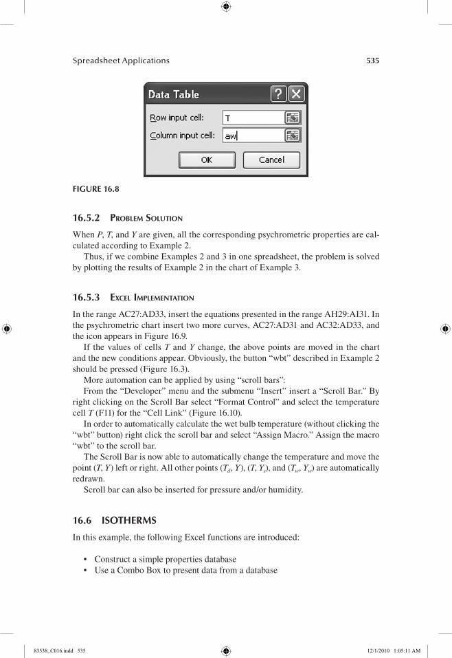
“What-if Analysis” select “Data Table.” The Data Table dialogue will appear (Figure 16.8).

4. In Data Table Dialogue assign cell “T” for the Row Input Cell and cell “aw” for the Column Input Cell. The corresponding values for humidity are auto-matically filled in the range S4:W25 (Figure 16.7).

Select the range R3:W25 shown in Figure 16.7 and from the menu “Insert” select the “Scatter” diagram. The psychrometric chart in Figure 16.7 is constructed.

16.5 calculatIonS on PSychrometrIc chart

In this example, the following Excel function is introduced:

• Use the scroll bar to change the values of a variable


In the psychometric chart of Example 3, select a point of given temperature and humidity (T, Y) and construct the corresponding dew point (Td, Y), the saturated point (T, Ys), and the wet bulb point (Tw, Yw).

I J K L M N1

VariableText

SymbolExcel Name Value Units Equation

2 Antoine equation constant for water a1

a1 a1. 1.19E+01 —


a2 a2. 3.99E+03 —


a3 a3. 2.34E+02 —

5 Air/water molecular weight ratio

m m 0.622 —

6 Water activity aw aw. 1.00 —7 Pressure P P. 1.00 bar8 Temperature T T. 65.00 °C9 Vapor pressure at

temperaturePs Ps. 0.249 bar :=EXP(a1.−a2./(a3.+T.) )

10 Humidity in vapor YV Yv. 0.206 kg/kg db :=m*aw.*Ps./(P.−aw.*Ps.)

FIgure 16.6

83538_C016.indd 533 12/1/2010 1:05:10 AM


P Q R S T U V W

Yv(T, aw)0.206 0.20 0.40 0.60 0.80 1.00

0 0.001 0.002 0.002 0.003 0.0045 0.001 0.002 0.003 0.004 0.006

10 0.002 0.003 0.005 0.006 0.00815 0.002 0.004 0.006 0.009 0.01120 0.003 0.006 0.009 0.012 0.01525 0.004 0.008 0.012 0.016 0.02030 0.005 0.011 0.016 0.022 0.02835 0.007 0.014 0.022 0.029 0.03740 0.009 0.019 0.029 0.039 0.05045 0.012 0.025 0.038 0.052 0.06650 0.016 0.032 0.050 0.068 0.08755 0.020 0.042 0.065 0.089 0.11660 0.026 0.054 0.084 0.117 0.15465 0.033 0.069 0.109 0.155 0.20670 0.041 0.088 0.142 0.205 0.27975 0.052 0.112 0.185 0.275 0.38680 0.065 0.144 0.244 0.375 0.55285 0.081 0.185 0.326 0.527 0.83690 0.100 0.240 0.445 0.779 1.41895 0.125 0.314 0.629 1.265 3.21599 0.150 0.394 0.864 2.145 19.447

123456789

10111213141617181920212223242527

I J K L M N111213141516171819

20

2122232425

2728293031323334353637

0.40

0.20

0.60

0.80

0.000

0.050

0.100

Hum

idity

(kg/

kg d

b)

0.150

0.200

0.250

0 10 20 30 40 50 60 70 80 90 100Temperature (°C)

Water activity = 1.00

26

FIgure 16.7

83538_C016.indd 534 12/1/2010 1:05:10 AM



When P, T, and Y are given, all the corresponding psychrometric properties are cal-culated according to Example 2.

Thus, if we combine Examples 2 and 3 in one spreadsheet, the problem is solved by plotting the results of Example 2 in the chart of Example 3.


In the range AC27:AD33, insert the equations presented in the range AH29:AI31. In the psychrometric chart insert two more curves, AC27:AD31 and AC32:AD33, and the icon appears in Figure 16.9.

If the values of cells T and Y change, the above points are moved in the chart and the new conditions appear. Obviously, the button “wbt” described in Example 2 should be pressed (Figure 16.3).

More automation can be applied by using “scroll bars”:From the “Developer” menu and the submenu “Insert” insert a “Scroll Bar.” By

right clicking on the Scroll Bar select “Format Control” and select the temperature cell T (F11) for the “Cell Link” (Figure 16.10).

In order to automatically calculate the wet bulb temperature (without clicking the “wbt” button) right click the scroll bar and select “Assign Macro.” Assign the macro “wbt” to the scroll bar.

The Scroll Bar is now able to automatically change the temperature and move the point (T, Y) left or right. All other points (Td, Y), (T, Ys), and (Tw, Yw) are automatically redrawn.

Scroll bar can also be inserted for pressure and/or humidity.

16.6 ISothermS


• Construct a simple properties database• Use a Combo Box to present data from a database

FIgure 16.8

83538_C016.indd 535 12/1/2010 1:05:11 AM



The equilibrium material moisture content Xe depends on air temperature, T and water activity, aw.

Various empirical or semitheoretical models have been proposed in the literature, but a modified Oswin model seems to be the most appropriate in process design calculations:

X b

b

T

a

ae

w

w

b

=+

−

12

273 1

3

exp( ) ( )

where b1, b2, and b3 are adjustable empirical constants, depending on the material characteristics.

The purpose of this example is to construct a database in an Excel environment to incorporate the Oswin constants for some materials and by using the various Excel

AA AB AC AD AE AF AG AH AI AJ AK AL AM

65 0.206 (T, Ys) : =T : =Ys65 0.035 (T, Y) : =T : =Y34 0.035 (Td, Y) : =Td : =Y65 0.035 (T, Y) : =T : =Y39 0.047 (Tw, Yw) : =Tw : =Yw

14

2728

30

123456789

10111213

151617181920212223242526

29

3132

(T, Ys)

(Td, Y)(T, Y)

(Tw, Yw)

0.20

0.40

0.60

0.80

0.000

0.050

0.100

0.150

0.200

0.250

0 10 20 30 40 50 60 70 80 90 100

Hum

idity

(kg/

kg d

b)

Temperature (°C)

Water activity = 1.00

FIgure 16.9

83538_C016.indd 536 12/1/2010 1:05:12 AM


utilities to construct an environment in which the moisture isotherms for various materials will be examined automatically.


Retrieve some values for the Oswin constants from the literature (e.g., Maroulis and Saravacos 2003) and insert these values in to an Excel spreadsheet as shown in the range B2:E6 in Figure 16.11.

Insert initial data values for the variables as follows:

jMaterial Material identification number

T Temperature

Aw Water activity

Insert the following equations for the following corresponding variable:

Name :=INDEX(Material,jMaterial)

b1. :=INDEX(Oswin1,jMaterial)



Xe :=b1.*EXP(b2./(273 + T))*(aw/(1-aw))∧b3.

The INDEX function selects a specific value from an array.

FIgure 16.10

83538_C016.indd 537 12/1/2010 1:05:12 AM


The following Excel names should be assigned in the following cells:

name cellaw C15

b1. C11

b2. C12

b3. C13

jMaterial C8

Material B3:B6

Oswin1 C3:C6

Oswin2 D3:D6

Oswin3 E3:E6

T C14

Xe C16

1

7

9

0.00

0.10

0.20

0.30

Equi

libriu

m m

ater

ial m

oist

ure

cont

ent (

kg/k

g db

)0.40

0.50

0.60

A B C D E F H I J K L M

2 Material Oswin1 Oswin2 Oswin33 Potato 3.27E–04 1.84E+03 4.00E–01

4.01E–013.89E–013.77E–01

1.75E+031.98E+031.83E+03

7.35E–044.01E–046.51E–04

4 Carrot5 Pepper6 Onion

8 jMaterial 1

Potatob1.b2.b3. 4.00E–01

1.84E+033.27E–04

Taw 0.25 –

65°C

Xe 0.05 kg/kg db

0.050.010.010.020.050.100.150.200.300.400.450.500.550.600.650.700.750.800.850.900.930.95

250.020.020.030.050.070.080.090.110.130.140.160.170.180.200.220.240.270.310.380.430.51

500.010.020.020.030.040.050.060.070.080.090.100.110.110.120.140.150.170.190.230.270.32

750.010.010.010.020.030.030.040.050.060.060.060.070.080.080.090.100.110.130.160.180.21

171819

10111213141516

2021222324252627282930313233343536

414243

37383940

0.00 0.20 0.40 0.60 0.80 1.00

Water activity

255075

Potato

Temperature (°C)

Potato

FIgure 16.11

83538_C016.indd 538 12/1/2010 1:05:13 AM


Insert a 2D Excel table using water activity values as the Column Input Cell and Temperature values as the Row Input Cell. The resulting table is shown in Figure 16.11.

Insert a Scatter Graph, as also shown in Figure 16.11, to graphically represent the results of the 2D Excel table.

Automate the material selection using a “Combo Box”:

• Insert a “Combo Box” from the menu “Developer” and submenu “Insert.”• Right click on the Combo Box and select “Format Control.”• In the “Format Control Dialogue,” assign the “Material” name to the “Input

Range” and the “jMaterial” name to the “Cell Link” (Figure 16.12).

The spreadsheet is now fully automated:By clicking the Combo Box, the available material appears in the Combo Box

List, and when a material is selected from the list, the material isotherms are auto-matically plotted in the Chart (Figure 16.11).

16.7 FIttIng rheologIcal data For chocolate


• Use matrix operations (Alt + Ctrl + Shift + ok)• Excel Solver

FIgure 16.12

83538_C016.indd 539 12/1/2010 1:05:13 AM



Analyze the rheological data on chocolate at 40°C, obtained in the COST 90 European project (Prentice and Huber 1983), using the Casson model:

τ τ γ= +( )/ /o1 2 1 2 2 Kc

whereτ (Pa) is the shear stressγ (1/s) is the shear rateτo and Kc are the Gasson constants

127.0To17Labs21.68Kc432Espx3

Shear stessexperimental

Shear stesscalculated

3435

A B C D E F G H

4 Lab Shear rate5 g Texp Tcal sd 14466 UCD 6.81 109 927 8.41 137 1018 13.64 182 130 Model9 29.11 217 203 Shear rate Shear stress

10 35.96 307 233 0.00512 2811 58.33 254 325 0.05 3112 72.20 462 379 0.1 3313 89.18 367 443 0.2 3514 4115 4716 5717 8018 11019 16120 29121 48322 83823 182724 277725 472627282930313233

36 0.34 50 3837 0.43 52 40

1

10

100

1,000

10,000

0.001

Shea

r str

ess (

Pa)

Shear rate (1/s)10001001010.10.01

FIgure 16.13

83538_C016.indd 540 12/1/2010 1:05:14 AM



In the spreadsheet in the Figure 16.13, 423 experimental data from 17 different labo-ratories are introduced in the range C6:D428.

Initial values for the Gasson constants are also introduced in the range H2:H3.In the range E6:E428, the calculated values using the Gasson model are intro-

duced using the equation:= (To∧0.5 + Kc*g∧0.5)∧2 in each cell.

The following Excel names should be assigned in the following cells:

name cellg C6:C428

Kc H3

sd H5

Tcal E6:E428

Texp D6:D428

To H2

The standard deviation between the experimental and calculated values is estimated in cell H5 by using the equation:

:={SQRT(SUM( (Texp-Tcal)∧2))}

Since Texp and Tcal are arrays, the mathematical operation in the cell refers to the matrix operation.

This is denoted by pressing Alt + Ctrl + Shift simultaneously when ok is clicked to end the equation editing. If the brackets {} exist in the equation, the matrix opera-tion has been accepted.

A comparison between the experimental and calculated values can be obtained by introducing the appropriate chart.

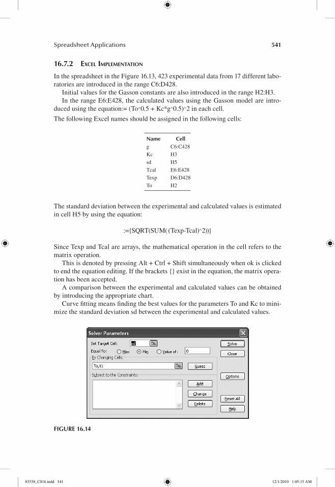
Curve fitting means finding the best values for the parameters To and Kc to mini-mize the standard deviation sd between the experimental and calculated values.

FIgure 16.14

83538_C016.indd 541 12/1/2010 1:05:15 AM


This operation can be performed using the Excel Solver:

• From the menu “Data” select “solver” and the Solver Parameters Dialogue will appear (Figure 16.14).

• Select the “min” operation, insert the variable “sd” in the “Set Target Cell” parameter, and the variables “To; Kc” in the “By Changing Cells” parameter.

• By pressing the button “Solve”, the optimization procedure is executed, and after some iteration, the optimal parameter estimates are obtained.

reFerenceS

Maroulis, Z.B. and Saravacos, G.D. 2003. Food Process Design. Marcel Dekker, New York.Prentice, J.H. and Huber, D. 1983. Results of the collaborative study on measuring rheo-

logical properties of foodstuffs. In: Physical Properties of Foods. R. Jowitt, F. Escher, B. Halstrom, H.F.Th. Meffert, W.E.L. Spiess, G, Vos, eds. Applied Science Publ., London, pp. 123–183.

Saravacos, G.D. and Maroulis, Z.B. 2001. Transport Properties of Foods. Marcel Dekker, New York.

83538_C016.indd 542 12/1/2010 1:05:15 AM

16 Spreadsheet Applications - MG Codemaroulis.mgcode.gr/wp-content/uploads/2013/05/fpeo16.pdf ·...

Documents

Transcript of 16 Spreadsheet Applications - MG Codemaroulis.mgcode.gr/wp-content/uploads/2013/05/fpeo16.pdf ·...